Abstract
Alpine grasslands face increasing threats from soil droughts due to climate change. While extensive research has focused on the direct impacts of drought on vegetation, the role of landscape fragmentation and spatiotemporal heterogeneity in shaping the response of these ecosystems to drought remains inadequately explored. This study aims to fill this gap by examining the Gannan alpine grassland in the northeastern Qinghai-Tibet Plateau. Using remote sensing data, indicators of spatial and temporal heterogeneity were derived, including spatial variance (SCV), spatial autocorrelation (SAC), and temporal autocorrelation (TAC). Two soil drought thresholds (Tr: threshold of rapid resistance loss and Tc: threshold of complete resistance loss) representing percentile-based drought intensities were identified to assess NDVI decline under drought conditions. Our findings indicate that the grassland has low resistance to soil droughts, with mean Tr and Tc of 8.93th and 7.36th percentile, respectively. Both increasing and decreasing spatiotemporal heterogeneity reduced vegetation resistance, with increasing SCV having a more pronounced effect. Specifically, increasing SCV increased Tr and Tc 1.4 times faster and 2.6 time slower than decreasing SCV, respectively. These results underscore the critical role of landscape heterogeneity in modulating grassland responses to drought, suggesting that managing vegetation patches could enhance ecosystem resilience.
1. Introduction
Grassland is a critical terrestrial ecosystem, covering approximately 40% of the global land surface and providing essential ecological services such as carbon sequestration and biodiversity preservation [1]. However, intensified climate change and anthropogenic activities have significantly impaired their resilience and stability, leading to widespread degradation [1,2]. This degradation is particularly pronounced in alpine grasslands, especially on the Qinghai-Tibet Plateau, a region characterized by extreme elevation and harsh climatic conditions, making it one of the most vulnerable ecosystems [3]. Alpine grasslands on the Qinghai-Tibet Plateau face unique challenges, including black soil land formation, disturbances from plateau pikas, and encroachment by invasive species, all of which exacerbate landscape fragmentation and spatiotemporal heterogeneity [4,5]. Such heterogeneity, marked by interlaced vegetation and bare soil patches [4], reflects ecosystem stability and vegetation growth dynamics [6]. Spatial heterogeneity indices have been proposed to assess the severity of alpine grassland degradation [7,8], but spatial heterogeneity itself plays a crucial role in mediating ecosystem function [9]. For instance, vegetation patch configuration (e.g., size, connectivity) directly regulates soil moisture retention, nutrient cycling, and microclimate buffering [9]. However, current ecological management often prioritizes homogeneous restoration targets, such as maximizing vegetation cover, while neglecting the functional role of spatial heterogeneity in stabilizing ecosystems under external stressors like soil droughts, which hinders the adaptive management under climate change.
Drought, a key climatic driver of ecosystem destabilization [10], triggers negative responses in vegetation, including productivity collapse, community structure disruption, and irreversible regime shifts [11,12,13,14]. Soil moisture depletion often accelerates degradation by surpassing critical thresholds linked to plant water stress and loss of resistance to drought [15,16]. On the Qinghai-Tibet Plateau, these thresholds vary spatially due to differences in vegetation types, species compositions, and landscape configurations [17]. Notably, ecosystems rarely respond linearly to drought intensity [18]; instead, their sensitivity depends on spatiotemporal heterogeneity to a certain extent [9]. For example, fragmented landscapes with high spatial heterogeneity may experience accelerated loss of resistance to drought once a threshold is exceeded, whereas more homogeneous landscapes may decline more gradually [17]. Degraded grasslands exhibit fragmented landscapes with altered soil moisture-nutrient feedbacks, whereas restored areas may show improved soil water retention [19,20]. While studies have mapped different drought thresholds [15,16], few explored how spatiotemporal heterogeneity affects their spatial distributions.
A critical yet often overlooked aspect of ecosystem management is designing vegetation patches while considering the asymmetric effects of spatiotemporal heterogeneity on responses to drought. Smaller or irregularly shaped vegetation patches experience amplified edge effects, leading to accelerated soil water evaporation and greater soil moisture loss compared to larger patches [21]. Increasing heterogeneity may initially enhance resource redistribution and biodiversity, but beyond a critical level, it can amplify sensitivity to drought [9,22]. Conversely, reducing heterogeneity might homogenize microenvironments, but might inadvertently lower resistance to extreme droughts. This asymmetry differs from traditional models that assume a uniform response to changes in heterogeneity. On the Qinghai-Tibet Plateau, landscape fragmentation is present in both degraded and restored alpine grasslands [8]. Although forest studies demonstrate that fragmented landscapes amplify ecosystem drought vulnerability [9,23], similar assessments for grasslands remain limited. When restoration efforts in management strategies prioritize vegetation coverage over spatial configuration, they neglect the importance of spatiotemporal heterogeneity and its functions, compromising long-term ecosystem resilience.
Advancements in remote sensing technology enable high-resolution mapping of soil moisture and vegetation heterogeneity [7], providing new opportunities to quantify ecosystem drought resistance. This study aims to address two key scientific questions: (1) How does landscape spatiotemporal heterogeneity affect soil drought thresholds in alpine grassland? (2) Do the asymmetric responses of drought resistance to changes in spatiotemporal heterogeneity require distinct management strategies for degraded versus restored landscapes? The hypothesis is that changes in spatiotemporal heterogeneity reduce ecosystem resistance to droughts by disrupting soil moisture stability and amplifying resource stress, with the sensitivity to these changes being asymmetric depending on whether heterogeneity increases or decreases. To test this, the study will identify two critical soil moisture thresholds associated with the loss of ecosystem resistance to drought and evaluate the relationships between spatiotemporal heterogeneity indices and these thresholds. By integrating threshold detection with landscape characteristics, our findings will enhance the understanding of grassland stability under climate change and inform management practices that combine vegetation recovery with spatially optimized designs to mitigate drought impacts.
2. Materials and Methods
2.1. Study Area
Gannan Prefecture, located in the Northeast Qinghai-Tibet Plateau (100°46′–104°44′E, 33°06′–36°10′N), is approximately 45,000 km2 with an average elevation exceeding 3000 m, descending westward to eastward (Figure 1). Characterized by a continental plateau climate, the region experiences an annual mean temperature of 1–3 °C and receives 400–800 mm of precipitation, predominantly occurring from May to September [24]. Grassland dominates the landscape (>55% coverage), including alpine meadow, steppe, sparse vegetation, shrub meadow, and wetland, primarily distributed across western and northern areas [25]. Forest occupies about 25% of the region, concentrated in the southeast. The growing season spans May to September [26], with an average temperature of 11 °C. As a pivotal pastoral-agricultural zone in China, Gannan’s economy remains fundamentally dependent on grassland-based livestock production. However, synergistic pressures from climate change and intensified human activities—particularly urban expansion and road infrastructure development—have driven grassland degradation and landscape fragmentation. This climate-vulnerable alpine ecosystem serves as a biodiversity reservoir with substantial carbon sequestration potential, and also a socio-ecological hotspot, in which traditional pastoralism conflicts with local ecological safety. These intersecting challenges underscore the urgent need to develop climate-resilient management frameworks for vulnerable grasslands under accelerating global change scenarios.
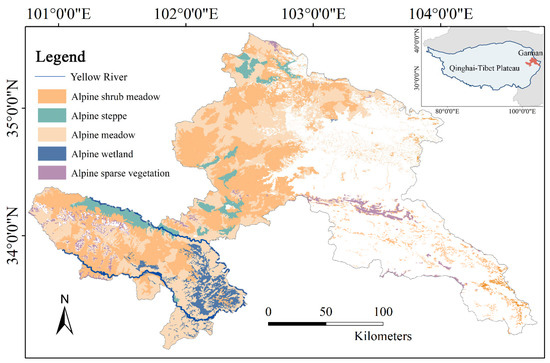
Figure 1.
Location of Gannan region and the distribution of alpine grassland types.
2.2. Data
2.2.1. Vegetation Index
As a common and qualified vegetation index, the Normalized Difference Vegetation Index (NDVI) was used to quantify vegetation growth dynamics. The gridded Moderate Resolution Imaging Spectroradiometer (MODIS) vegetation indices from the U.S. National Aeronautics and Space Administration (NASA) (MOD13A2 and MOD13Q1; 16-day temporal resolution) were acquired and preprocessed via the Google Earth Engine (GEE) platform [8,27]. The datasets provide NDVI at spatial resolutions of 1 km for MOD13A2 and 250 m for MOD13Q1, respectively. Annual and monthly NDVI composites from 2000 to 2020 were generated using the Maximum Value Composite (MVC) method to mitigate noise from clouds, atmospheric interference, and solar altitude angle [28]. Missing values and anomalies in the NDVI time series were rectified through per-pixel linear interpolation [29].
2.2.2. Soil Moisture
Surface soil moisture data (2000–2020) were obtained from the National Tibetan Plateau Data Center for soil drought assessment. This validated product combines ESA-CCI SSM and ERA5 reanalysis datasets and downscaled using Random Forest algorithm [30]. The data spatial resolution is 1 km, which is same as MOD13A2.
2.2.3. Auxiliary Data
Grassland boundaries in Gannan region were derived from the 30 m resolution GlobeLand30 V2020 product, developed by the National Geomatics Centre of China, with recent ground–truth adjustments. Vegetation types were classified based on the 1:500,000-scale Vegetation map of the Qinghai Tibet Plateau (2020) [31]. Non-grassland areas (forests, cultivated plants, water bodies, and non-vegetated zones) were masked during analysis (Figure 1).
All data used are shown in Table 1.

Table 1.
The dataset used in this study.
2.3. Methods
2.3.1. Soil Drought Resistance Evaluation
The assessment of soil drought resistance was conducted by identifying critical soil moisture thresholds associated with vegetation degradation signals. Monthly soil moisture data during growing seasons (May to September) from 2000 to 2020 were initially processed to derive statistical parameters (mean, variance, and standard deviation, σ). For each pixel, soil drought events were defined as values falling below one standard deviation (−1.0σ) from the mean moisture level [16]. Vegetation degradation events were identified when NDVI values exhibited an abrupt 10% decrease relative to the preceding month. Subsequently, the spatiotemporal coincidence probability between soil drought events and NDVI decline events was quantified through statistical co-occurrence analysis. However, equivalent soil drought intensities did not universally trigger NDVI reduction, indicating differential ecosystem resistance to moisture stress [32]. Therefore, soil drought thresholds could be determined by quantifying the coincidence rate (r) between soil moisture deficit magnitudes and corresponding NDVI response frequencies [33,34]. The coincidence rate r was calculated using the equation:
where Fre means the frequency of each event that has occurred, means the events of abnormal decline of NDVI according to the definition above, and means the events of soil moisture below the specific soil drought intensity.
Soil drought intensity was described using the percentile in surface soil moisture. Based on the statistical distribution of soil moisture data, soil drought intensities were discretized across a gradient from extreme drought (low percentile) to slight drought (high percentile) to capture nonlinear response patterns. Pixel-scale nonlinear regression models were subsequently fitted to characterize the relationship between drought intensity gradients and vegetation response probabilities [16]. For pixels with more than three co-occurrence events of soil drought and NDVI decline, two critical thresholds were identified: complete resistance loss threshold Tc and rapid resistance loss threshold Tr (the hypothesis curve is in Supplementary Figure S1). Tc was identified by the inflection point where r approaches 100%, indicating ecosystem resistance collapse under soil drought stress. Tr was identified by curvature analysis, when the first derivative of the response curve equals the slope between maximum and minimum r values, representing the initiation of accelerated resistance decline. Higher Tc/Tr values indicate higher vegetation vulnerability and lower vegetation resistance, where limited soil moisture reduction triggers NDVI loss, and vice versa.
2.3.2. Spatial and Temporal Heterogeneity Indicators
Spatial coefficient of variance (SCV) and Moran’s I-based spatial autocorrelation (SAC) were used as spatial heterogeneity indicators to characterize alpine grassland vegetation patterns [7,27]. Both indicators were computed using 4 × 4 pixel (1 km2) moving windows on MOD13Q1 NDVI datasets. The formula of SCV calculation is as follows:
where means the mean NDVI values of 16 pixels in the moving window, is the NDVI value of each pixel in the moving window, and n is the number of pixels in the moving window which equals 16 here.
The spatial autocorrelation is calculated using the global Moran’ I, and the formula is as follows:
where is the spatial weight matrix based on adjacency relationship, and others have the same meanings with SCV.
Temporal autocorrelation (TAC) was assessed using the lag-1 autoregressive model (AR(1)) applied to detrended and deseasonalized MOD13A2 NDVI series. A sliding 5-year window (60 monthly composites) with monthly increments quantified landscape pattern persistence [35]. TAC was calculated as follows:
where is the TAC coefficient, and are the NDVI values at time t and t + 1, and ε is residual.
2.3.3. Statistical Analysis
Linear least-squares regression was used to quantify pixel-level temporal trends of spatiotemporal heterogeneity indices. The slope () was calculated as:
where n is the quantity of data for the regression, and is the spatial or temporal heterogeneity index value at time t.
Both linear and quadratic polynomial models were employed to characterize the relationship between heterogeneity dynamics (slope coefficients) and soil drought thresholds (Tr/Tc). Given the high dimensionality of the study area, the analysis employed quantile-based discretization: (1) the slope () and annual average value of each heterogeneity index were partitioned into 100 equidistant percentile bins; (2) minimum soil drought threshold within each bin was extracted as the target variable. This generated 100 paired datasets for regression analysis. Bins lacking valid drought threshold measurements were excluded from subsequent model fitting to ensure statistical robustness. The linear fitting model for soil drought threshold T is described as:
The quadratic polynomial model is described as:
where x represents the mean value of each data piece; a and b are the coefficients of linear fitting; c, d, and e are the coefficients of quadratic curve fitting; and and are residuals.
3. Results
3.1. Spatial Distribution of Soil Drought Thresholds
The identification of soil droughts (0.83 ± 0.12 events/year) and NDVI degradation events (0.79 ± 0.18 events/year) revealed distinct spatial clustering patterns (Figure 2). Soil moisture deficits predominantly occurred in the southwestern areas adjacent to the Yellow River and northwestern zones, whereas vegetation degradation exhibited inverse results near the Yellow River (Figure 1 and Figure 2). The alpine meadow and alpine shrub meadow ecosystems in the southwest with higher elevations demonstrated more NDVI decline events than others.
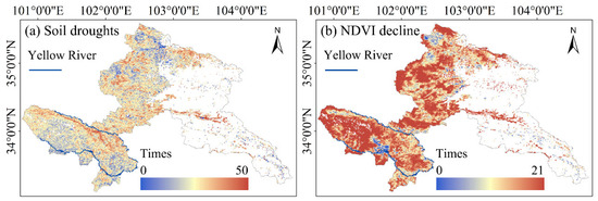
Figure 2.
Occurrence of abnormal events. (a) Occurrence of soil drought events; (b) Occurrence of abnormal NDVI decline events. The blank areas are non-grassland areas and areas without sufficient data for calculation.
The comparison of model fitting demonstrated that exponential functions outperformed (higher R2) linear models across 70.08% pixels with sufficient observational data (Supplementary Figure S2), indicating prevalent nonlinear responses of alpine grassland to intensifying drought stress. The rapid resistance loss threshold Tr had a mean value of 8.93th, with low values clustered in western alpine shrub meadows and sparse vegetation zones with high elevation, whereas riparian zones and alpine wetlands showed higher thresholds (Figure 1 and Figure 3a). Similarly distributed, the complete resistance loss threshold Tc averaged at 7.36th. The northern alpine steppes had comparatively higher Tc values relative to alpine meadows and shrub meadows (Figure 1 and Figure 3b). Geographically, southern regions—particularly alpine meadows and shrub meadows in Figure 1—had higher Tc thresholds than the north. Collectively, these patterns indicate the vulnerability of Gannan’s alpine grasslands, where minor soil moisture deficits triggered rapid ecosystem resistance degradation. The narrow threshold interval between two thresholds further suggests accelerated resistance depletion post–initial drought triggering.
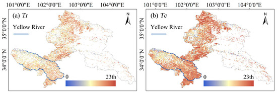
Figure 3.
Spatial distribution of soil drought thresholds Tr (a) and Tc (b). Higher percentile of thresholds means lower resistance to soil droughts.
3.2. Changing Trends of Spatiotemporal Heterogeneity Indicators
NDVI exhibited minimal temporal variation (mean slope: 0.0012), with growing seasons averaged at 0.68. Notably, northern low-elevation and southwestern high-altitude grasslands demonstrated low NDVI baselines, while enhanced recovery trends were observed (Figure 4a and Figure 5a). SCV maintained near-stationary dynamics (mean slope ≈ 0), though localized increases emerged in riparian zones spatially contrasting with decreases in the northern region (Figure 1 and Figure 4b). SCV averaged at 0.046, and most regions with lower SCV values exhibited positive trends, whereas higher SCV values corresponded to reduction trends (Figure 4b and Figure 5b). SAC displayed non-directional temporal patterns with global mean slope approximating zero (Figure 4c), yet a general spatial aggregated performance (mean: 0.30) characterized in the whole area, particularly in northern and southwestern zones (Figure 5c).
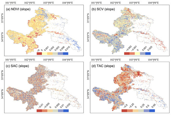
Figure 4.
Temporal trends (slope) of NDVI and spatiotemporal indicators of Gannan alpine grassland. (a) NDVI; (b) Spatial variance (SCV); (c) Spatial autocorrelation (SAC); (d) Temporal autocorrelation (TAC). The blank areas are non-grassland areas and areas without sufficient data for calculation.
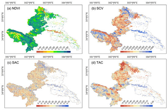
Figure 5.
Annual average values of NDVI and spatiotemporal indicators of Gannan alpine grassland. (a) NDVI; (b) Spatial variance (SCV); (c) Spatial autocorrelation (SAC); (d) Temporal autocorrelation (TAC). The blank areas are non-grassland areas and areas without sufficient data for calculation.
TAC revealed a weak system memory (mean slope: −0.086), indicating gradual divergence from historical growth patterns. Southwestern and far-northern regions showed higher TAC baselines and steeper slopes (Figure 4d and Figure 5d). Predominantly negative TAC values (global mean: −0.32) showed the self-regulating ability of the ecosystem under soil droughts across most areas.
Given SAC’s limited spatial discriminability at 1 km resolution, subsequent analyses focused on NDVI, SCV, and TAC. Divergent trends dominated pairwise comparisons: 60.66% of the study area exhibited inverse NDVI-SCV relationships, as well as 58.46% for NDVI-TAC relationships, while 54.08% demonstrated SCV-TAC covariation (Table 2).
Table 2.
Percentages of the area with positive (+) or negative (−) changing trends of NDVI, spatial variance (SCV), and temporal autocorrelation (TAC).
3.3. Influences of Spatiotemporal Heterogeneity to Drought Resistance
The minimum soil drought thresholds (Tr and Tc) were analyzed against temporal trends of three spatiotemporal heterogeneity indicators (SCV, SAC, TAC) using quadratic curve fitting firstly (Figure 6). Rapidly changed SCV (Tr: >0.005 or <−0.005; Tc: >0.006 or <−0.008), SAC (Tr: >0.02 or <−0.02; Tc: >0.02 or <−0.02), and TAC (Tr: >0.7 or <−0.7; Tc: >0.7) exhibited significantly depressed thresholds, suggesting that accelerated spatiotemporal heterogeneity changes reduce vegetation resistance. All six scenarios showed peak drought thresholds when heterogeneity trends approached zero. However, asymmetric responses emerged that negative heterogeneity trends (slope < 0) reduced drought resistance with different rate compared to equivalent positive trends.
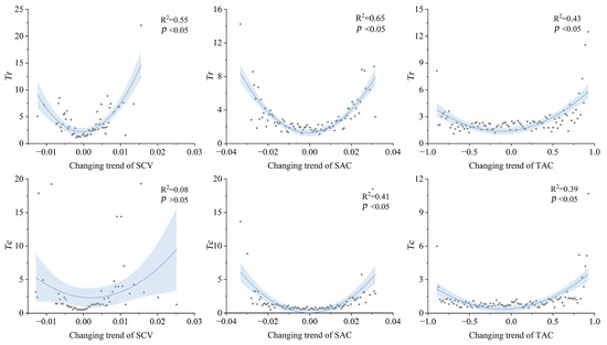
Figure 6.
Quadric curve fitting for the changing trends of three indicators (spatial variance (SCV), spatial autocorrelation (SAC), and temporal autocorrelation (TAC)) and two soil drought thresholds (Tr and Tc). The shaded areas mean the 95% confidence interval. The unit of Tr and Tc are percentile of soil moisture.
Piecewise linear modeling delineated direction-dependent effects (Figure 7, and the residual tests were shown in Supplementary Figure S3 to S8). Increasing SCV triggered 1.4× faster Tr increase but 2.6× slower Tc increase than decreasing SCV. For SAC, quadratic polynomial models outperformed piecewise fits, indicating symmetric decline rates across the changing gradients, and reflecting balanced resistance responses to aggregation/dispersion force. Similar with SCV, increasing TAC triggered 2.7× faster Tr increase and 2.6× faster Tc increase than decreasing TAC.
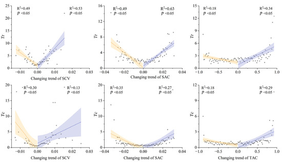
Figure 7.
Piecewise linear fitting for the temporal changing trends of three indicators (spatial variance (SCV), spatial autocorrelation (SAC), and temporal autocorrelation (TAC)) and two soil drought thresholds (Tr and Tc) with the meeting points where changing trends equaled zero. The shaded areas mean the 95% confidence interval. The unit of Tr and Tc are percentile of soil moisture.
Figure 8 illustrates the relationships between annual mean values of the three spatiotemporal heterogeneity indicators (SCV, SAC, TAC) and the two soil drought thresholds (Tr, Tc). Vegetation resistance exhibited an inverse relationship with SCV, which declined as SCV increased, and the resistance decreased obviously when SCV was larger than 0.3. Similarly, SAC and TAC also demonstrated nonlinear relations with drought thresholds. SAC reached peak resistance values at 0.35 (Tr) and 0.32 (Tc), while TAC peaked at −0.36 (Tr) and −0.35 (Tc). These nonlinear patterns suggest that moderately aggregated spatial configurations and intermediate temporal heterogeneity may optimize vegetation resistance to soil drought stress.
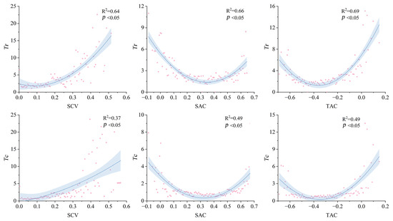
Figure 8.
Quadric curve fitting for annual average values of three indicators (spatial variance (SCV), spatial autocorrelation (SAC), and temporal autocorrelation (TAC)) and two soil drought thresholds (Tr and Tc). The shaded areas mean the 95% confidence interval. The unit of Tr and Tc are percentile of soil moisture.
4. Discussion
4.1. Landscape Heterogeneity Dynamics in Degradation-Restoration Progress
Landscape heterogeneity shows variations corresponding to grassland growth status. Grassland degradation is a retrogressive succession process influenced by both natural and anthropogenic factors, while restoration typically involves human-led replantation, sometimes aided by climate change [36]. Both degradation and restoration affect plant coverage, vegetation productivity, and landscape patterns. Conventional indicators including NDVI, NPP, and LAI exhibit significant changes with shifts in grassland ecosystem status [37]. Additionally, vegetation fragmentation and landscape heterogeneity effectively indicate grassland growth status, but their temporal trajectories may diverge from NDVI or NPP fluctuations [7].
Alpine grassland landscapes, especially degraded ones, are predominantly characterized by vegetation patches interspersed with bare soil areas. This spatial configuration and accompanying heterogeneity result from bioturbation, vegetation loss, species invasion, and abiotic drivers [38]. Healthy grasslands typically display homogeneous landscapes containing randomly distributed vegetation patches.
During degradation, there is a reduction in vegetation patches along with an expansion in bare soil coverage, leading to fluctuating SCV. Initially, SCV increases as vegetation patterns transition to bare soils; it then decreases if degradation progresses, resulting in more extensive bare soil areas. Similarly, during restoration, SCV increases as the landscape shifts from non-vegetated to low-vegetation states and decreases as the grassland improves toward intact conditions. In this study, SAC, which reflects the randomness of vegetation distribution, did not exhibit a clear changing pattern. This may be due to scale limitations, as the global Moran’s I is typically applied in regional-scale analyses [27]. TAC indicates an ecosystem’s propensity to maintain historical states [39]. An increase in TAC generally suggests ongoing degradation from an already degraded state, while a decrease indicates a mix of vegetation and bare soil patches and transitions between degradation and restoration. Furthermore, in areas where changes in spatiotemporal heterogeneity were not statistically significant, it suggests that the variability in vegetation patterns remained stable over time. Such stability may indicate consistent environmental conditions or the resilience of the ecosystem to disturbances, as spatial heterogeneity has been linked to increased diversity and stability in grassland communities [40].
Landscape heterogeneity can also indicate the establishment and proliferation of invasive species. While vegetation coverage is often used as an indicator of grassland degradation, species invasion can complicate this relationship by affecting vegetation indices such as NDVI or EVI [8]. Invasive species may exhibit higher plant cover than native species while maintaining patch-bare soil mosaics [41,42]. Consequently, invasive species can increase overall vegetation coverage, masking underlying degradation [43]. In such cases, landscape heterogeneity tends to increase alongside vegetation indices, even though the grassland may be in a slightly degraded state.
4.2. Impact of Landscape Heterogeneity on Soil Drought Thresholds
The study reveals that landscape spatiotemporal heterogeneity significantly modulates soil drought thresholds in alpine grasslands, directly addressing the first research question. During both degradation and restoration processes, we observed fluctuations in SCV, SAC, and TAC of vegetation index. These heterogeneity fluctuations fundamentally determine the soil moisture levels triggering vegetation water stress, defined as soil drought thresholds [21]. The observed relationships originate from underlying ecohydrological processes.
Our findings demonstrate that higher SCV was associated with lower drought resistance, indicating that grasslands with greater spatial variation in vegetation cover are more vulnerable to drought impacts. This phenomenon is likely due to uneven water distribution, where sparsely vegetated areas experience higher evaporation rates and reduced soil moisture retention [44]. Higher SCV leads to greater variation in soil moisture across the landscape, where bare soil patches experience faster drying and higher temperatures to exacerbate water stress for adjacent vegetation. Higher SAC, which indicates more aggregated vegetation patches, was supposed to have higher drought resistance. Because large, contiguous patches have the ability to retain water and nutrients more effectively, they create microenvironments with improved soil structure, higher organic matter, and better water infiltration rates that buffer against drought conditions [45]. Contrary to theoretical expectations, SAC showed no significant effect on drought thresholds in this study. This discrepancy may reflect ecosystem instability in artificially restored areas where rapid SAC increases occur without concomitant ecological design. Similarly, moderate TAC levels may facilitate beneficial water-nutrient redistribution across growing seasons, whereas extreme TAC fluctuations from anthropogenic disturbances likely destabilize systems through intensified vegetation–soil alternation [46]. Moreover, spatiotemporal heterogeneity influences microclimatic conditions. Large patches demonstrate superior capacity for evapotranspiration reduction through shading and windbreak effects, particularly important in alpine environments with pronounced temperature fluctuations. More aggregated landscapes may support higher species richness within patches, leading to greater functional diversity and, consequently, enhanced resistance to environmental stressors through complementary resource use [47]. Comparatively, our findings align with previous studies. The detected drought threshold percentile slightly exceeds values reported in China, where the average Tr was 8.7th [48], suggesting superior drought resistance in alpine grasslands. While few studies explicitly link landscape heterogeneity with vegetation drought resistance, our observations parallel Schwartz et al. [9]’s report on forest, a pattern mirrored in our study of alpine grasslands, where fragmented forest landscapes exhibit increased vulnerability to drought. However, differences may arise due to scale or indicators. For instance, Wu et al. [49] identified contrasting thermal buffering capacities in fragmented grasslands, highlighting context-dependent heterogeneity effects requiring further investigation.
The hypothesis of asymmetric sensitivity in drought resistance to changes in heterogeneity is also supported. Specifically, increases in SCV during the early stages of degradation lead to a rapid decline in drought resistance, while decreases in SCV during restoration do not necessarily restore resistance to its original levels immediately, suggesting a hysteresis effect [50]. Furthermore, the impact of TAC on resistance also exhibited asymmetry. Increasing TAC may decrease resistance faster than reducing temporal similarity in already degraded areas. This implies that management strategies should be tailored to the specific context of the landscape’s degradation or restoration status.
4.3. Implications and Uncertainties
This study underscores the critical role of landscape heterogeneity in alpine grassland management, particularly under increasing drought frequency due to climate change. Grassland landscape heterogeneity or landscape fragmentation usually appears due to changes in grassland growth status and land use/land cover which has been significantly affected by anthropogenic activities [46]. To enhance drought resistance, management strategies should aim to optimize spatial configurations of vegetation patches. For degraded landscapes characterized by rapidly changing SCV and increasing SAC, interventions should focus on promoting the aggregation of vegetation patches to maximize water retention and minimize edge effects, such as strategic planting or fencing to allow natural regeneration in contiguous areas. In restored areas, maintaining a balance between heterogeneity and homogeneity is key. Excessive uniformity may reduce biodiversity and functional redundancy, while extreme heterogeneity may undermine ecological resistance [51]. It should be noticed that ecosystem resistance and stability might decrease due to the rapid changing of patch types and sizes even in the restoration process. An optimal configuration involves continuous alpine grassland expansion with stochastic emergence of supplementary patches. Increasing grassland aggregation and partitioning overlarge vegetation patches are both good ways to promote vegetation productivity, soil conservation, and water retention [52], and finally decrease the ecosystem vulnerability to soil droughts. Implementing adaptive management practices that monitor and adjust landscape configurations based on ongoing climatic trends and ecosystem responses will safeguard long-term stability and functionality [53].
However, there are uncertainties in this study. First, we did not account for microtopographic features such as slope aspect and soil depth, which can significantly influence water retention and distribution. Future research should incorporate these variables to refine the understanding of how landscape heterogeneity interacts with topography. Second, species composition effects remain unaddressed, despite its potential to modulate ecosystem responses. Different plant species have varying water use efficiencies and drought tolerances, which can affect overall resistance [54]. Integrating species-level data could enhance threshold detection precision. Third, our reliance on MODIS NDVI data at 1 km and 250 m resolution, along with specific moving window sizes, may overlook fine-scale heterogeneity within pixels and moving windows. To address this limitation, future research could utilize higher-resolution sensors such as Landsat or Sentinel, or conduct field measurements to gain more detailed insights into pixel-scale dynamics. Moreover, challenges like NDVI saturation and cloud contamination can be tackled by integrating data from various remote sensors and employing different vegetation indices. However, a persistent challenge for future studies remains in handling the discrepancy in spatial resolution between vegetation index data and soil moisture data. Besides, although linear interpolation was used to reliably fill in minimal missing data [29,55], it is crucial to emphasize that data integrity is fundamental to the accuracy of the results. Next, temporal lag effects were excluded based on Wang et al. [56]’s findings of weak vegetation-drought response delays in Gannan grasslands. Nevertheless, investigating longer lag periods may be necessary to elucidate the hysteretic responses of landscape heterogeneity to soil moisture deficits. Finally, human activities, including grazing and restoration practices, introduce uncertainties that were not fully controlled in our study. More detailed data on management intensities and spatial distributions would improve robustness, acknowledging the influence of anthropogenic factors on landscape heterogeneity and drought resistance.
5. Conclusions
This study identified two soil drought thresholds, Tr for rapid resistance loss and Tc for complete resistance loss, to assess vegetation resistance to soil droughts in Gannan’s alpine grasslands. We employed two spatial heterogeneity metrics—spatial coefficient of variation (SCV) and spatial autocorrelation (SAC)—and one temporal autocorrelation indicator (TAC) to quantify landscape fragmentation dynamics. The results showed that the grasslands had low resistance, with averaged Tr at the 8.93th and Tc at the 7.36th percentile of soil moisture, and spatiotemporal heterogeneity was dynamic across the region. Both rapid increases and decreases in heterogeneity reduced resistance, with asymmetrical effects, where higher SCV lowered resistance, while slight SAC and moderate TAC could enhance it. These findings highlight the functional significance of landscape fragmentation patterns and spatiotemporal heterogeneity in ecosystem management frameworks. Under climate change scenarios, alpine grassland management should prioritize heterogeneity optimization to enhance drought resilience. Specifically, keeping SCV low by reducing variability in vegetation cover can help, such as through restoring degraded areas to ensure more uniform cover. Promoting slight spatial aggregation, like designing connected vegetation patches, can also support resilience by facilitating species movement and resource sharing. Monitoring TAC is crucial to maintain moderate similarity to past conditions, avoiding rapid changes that might destabilize the ecosystem.
Supplementary Materials
The following supporting information can be downloaded at: https://www.mdpi.com/article/10.3390/rs17071293/s1, Figure S1: Hypothesis curve two soil drought thresholds; Figure S2: Higher R2 of curving fitting for Tr calculation. Two fitting methods were compared, including linear fitting and exponential fitting; Figure S3: Residual test for linear fitting of SCV trends and Tr; Figure S4: Residual test for linear fitting of SCV trends and Tc; Figure S5: Residual test for linear fitting of SAC trends and Tr; Figure S6: Residual test for linear fitting of SAC trends and Tc; Figure S7: Residual test for linear fitting of TAC trends and Tr; Figure S8: Residual test for linear fitting of TAC trends and Tc.
Author Contributions
Conceptualization, Y.W. and H.L.; Data curation, Y.W. and J.J.; Funding acquisition, Z.H.; Methodology, Y.W. and W.Z.; Project administration, H.L. and Z.H.; Resources, J.J. and Z.H.; Software, Y.W.; Supervision, H.L. and W.Z.; Validation, Y.W. and H.L.; Visualization, Y.W.; Writing—original draft, Y.W.; Writing—review & editing, H.L. and W.Z. All authors have read and agreed to the published version of the manuscript.
Funding
This research was jointly supported by the Major Science and Technology Projects of Gansu Province (21ZD4FA020), the Leading Talents Program of Gansu Province (E339040101), and the National Natural Science Foundation of China (42171117).
Data Availability Statement
The dataset mentioned in the manuscript can be obtained from the website in this paper.
Conflicts of Interest
The authors declare no conflicts of interest.
Abbreviations
The following abbreviations are used in this manuscript:
| NDVI | Normalized Difference Vegetation Index |
| GEE | Google Earth Engine |
| MODIS | Moderate Resolution Imaging Spectroradiometer |
| SM | Soil moisture |
| SCV | Spatial variance |
| SAC | Spatial autocorrelation |
| TAC | Temporal autocorrelation |
References
- Bardgett, R.D.; Bullock, J.M.; Lavorel, S.; Manning, P.; Schaffner, U.; Ostle, N.; Chomel, M.; Durigan, G.; Fry, E.L.; Johnson, D. Combatting global grassland degradation. Nat. Rev. Earth Environ. 2021, 2, 720–735. [Google Scholar] [CrossRef]
- de Bello, F.; Lavorel, S.; Hallett, L.M.; Valencia, E.; Garnier, E.; Roscher, C.; Conti, L.; Galland, T.; Goberna, M.; Májeková, M.; et al. Functional trait effects on ecosystem stability: Assembling the jigsaw puzzle. Trends Ecol. Evol. 2021, 36, 822–836. [Google Scholar] [CrossRef] [PubMed]
- Yan, Z.; Gao, Z.; Sun, B.; Ding, X.; Gao, T.; Li, Y. Global degradation trends of grassland and their driving factors since 2000. Int. J. Digit. Earth 2023, 16, 1661–1684. [Google Scholar] [CrossRef]
- Gao, J.; Li, X. A knowledge-based approach to mapping degraded meadows on the Qinghai–Tibet Plateau, China. Int. J. Remote Sens. 2017, 38, 6147–6163. [Google Scholar] [CrossRef]
- Qian, D.; Li, Q.; Fan, B.; Lan, Y.; Cao, G. Characterization of the spatial distribution of plateau pika burrows along an alpine grassland degradation gradient on the Qinghai–Tibet Plateau. Ecol. Evol. 2021, 11, 14905–14915. [Google Scholar] [CrossRef]
- Kéfi, S.; Rietkerk, M.; Alados, C.L.; Pueyo, Y.; Papanastasis, V.P.; ElAich, A.; De Ruiter, P.C. Spatial vegetation patterns and imminent desertification in Mediterranean arid ecosystems. Nature 2007, 449, 213–217. [Google Scholar] [CrossRef]
- Li, C.; Jong, R.D.; Schmid, B.; Wulf, H.; Schaepman, M.E. Changes in grassland cover and in its spatial heterogeneity indicate degradation on the Qinghai-Tibetan Plateau. Ecol. Indic. 2020, 119, 106641. [Google Scholar] [CrossRef]
- Wang, Y.; Liu, H.; Zhao, W.; Jiang, J.; He, Z.; Yu, Y.; Guo, L.; Yetemen, O. Early warning signals of grassland ecosystem degradation: A case study from the northeast Qinghai-Tibetan Plateau. Catena 2024, 239, 107970. [Google Scholar] [CrossRef]
- Schwartz, N.B.; Budsock, A.M.; Uriarte, M. Fragmentation, forest structure, and topography modulate impacts of drought in a tropical forest landscape. Ecology 2019, 100, e02677. [Google Scholar] [CrossRef]
- Vicente-Serrano, S.M.; Quiring, S.M.; Peña-Gallardo, M.; Yuan, S.; Domínguez-Castro, F. A review of environmental droughts: Increased risk under global warming? Earth Sci. Rev. 2020, 201, 102953. [Google Scholar] [CrossRef]
- Piao, S.; Zhang, X.; Chen, A.; Liu, Q.; Lian, X.; Wang, X.; Peng, S.; Wu, X. The impacts of climate extremes on the terrestrial carbon cycle: A review. Sci. China Earth Sci. 2019, 62, 1551–1563. [Google Scholar] [CrossRef]
- Clark, J.S.; Iverson, L.; Woodall, C.W.; Allen, C.D.; Bell, D.M.; Bragg, D.C.; D’Amato, A.W.; Davis, F.W.; Hersh, M.H.; Ibanez, I.; et al. The impacts of increasing drought on forest dynamics, structure, and biodiversity in the United States. Glob. Change Biol. 2016, 22, 2329–2352. [Google Scholar] [CrossRef] [PubMed]
- Orimoloye, I.R.; Belle, J.A.; Ololade, O.O. Drought disaster monitoring using MODIS derived index for drought years: A space-based information for ecosystems and environmental conservation. J. Environ. Manag. 2021, 284, 112028. [Google Scholar] [CrossRef]
- Li, C.; Fu, B.; Wang, S.; Stringer, L.C.; Zhou, W.; Ren, Z.; Hu, M.; Zhang, Y.; Rodriguez-Caballero, E.; Weber, B. Climate-driven ecological thresholds in China’s drylands modulated by grazing. Nat. Sustain. 2023, 6, 1363–1372. [Google Scholar] [CrossRef]
- Fu, Z.; Ciais, P.; Wigneron, J.-P.; Gentine, P.; Feldman, A.F.; Makowski, D.; Viovy, N.; Kemanian, A.R.; Goll, D.S.; Stoy, P.C.; et al. Global critical soil moisture thresholds of plant water stress. Nat. Commun. 2024, 15, 4826. [Google Scholar] [CrossRef]
- Piao, Z.; Li, X.; Xu, H.; Wang, K.; Tang, S.; Kan, F.; Hong, S. Threshold of climate extremes that impact vegetation productivity over the Tibetan Plateau. Sci. China Earth Sci. 2024, 67, 1967–1977. [Google Scholar] [CrossRef]
- Zhang, Y.; Hong, S.; Liu, D.; Piao, S. Susceptibility of vegetation low-growth to climate extremes on Tibetan Plateau. Agric. Meteorol. 2023, 331, 109323. [Google Scholar] [CrossRef]
- Li, W.; Yan, D.; Weng, B.; Lai, Y.; Zhu, L.; Qin, T.; Dong, Z.; Bi, W. Nonlinear effects of surface soil moisture changes on vegetation greenness over the Tibetan plateau. Remote Sens. Environ. 2024, 302, 113971. [Google Scholar] [CrossRef]
- Xu, Y.; Dong, S.; Gao, X.; Yang, M.; Li, S.; Shen, H.; Xiao, J.; Han, Y.; Zhang, J.; Li, Y.; et al. Aboveground community composition and soil moisture play determining roles in restoring ecosystem multifunctionality of alpine steppe on Qinghai-Tibetan Plateau. Agric. Ecosyst. Environ. 2021, 305, 107163. [Google Scholar] [CrossRef]
- Pan, T.; Hou, S.; Liu, Y.; Tan, Q.; Liu, Y.; Gao, X. Influence of degradation on soil water availability in an alpine swamp meadow on the eastern edge of the Tibetan Plateau. Sci. Total Environ. 2020, 722, 137677. [Google Scholar] [CrossRef]
- Zhang, W.; Yi, S.; Qin, Y.; Sun, Y.; Shangguan, D.; Meng, B.; Li, M.; Zhang, J. Effects of Patchiness on Surface Soil Moisture of Alpine Meadow on the Northeastern Qinghai-Tibetan Plateau: Implications for Grassland Restoration. Remote Sens. 2020, 12, 4121. [Google Scholar] [CrossRef]
- Gómez-Fernández, D.; López, R.S.; Zabaleta-Santisteban, J.A.; Medina-Medina, A.J.; Goñas, M.; Silva-López, J.O.; Oliva-Cruz, M.; Rojas-Briceño, N.B. Landsat images and GIS techniques as key tools for historical analysis of landscape change and fragmentation. Ecol. Inform. 2024, 82, 102738. [Google Scholar] [CrossRef]
- Xie, Y.; Li, J.; Wulan, T.; Zheng, Y.; Shen, Z. Scale dependence of forest fragmentation and its climate sensitivity in a semi-arid mountain: Comparing Landsat, Sentinel and Google Earth data. Geogr. Sustain. 2024, 5, 200–210. [Google Scholar] [CrossRef]
- Ma, P.; Zhao, J.; Zhang, H.; Zhang, L.; Luo, T. Increased precipitation leads to earlier green-up and later senescence in Tibetan alpine grassland regardless of warming. Sci. Total Environ. 2023, 871, 162000. [Google Scholar] [CrossRef]
- Liu, C.; Li, W.; Zhu, G.; Zhou, H.; Yan, H.; Xue, P. Land Use/Land Cover Changes and Their Driving Factors in the Northeastern Tibetan Plateau Based on Geographical Detectors and Google Earth Engine: A Case Study in Gannan Prefecture. Remote Sens. 2020, 12, 3139. [Google Scholar] [CrossRef]
- Wang, Y.; Xiao, J.; Ma, Y.; Ding, J.; Chen, X.; Ding, Z.; Luo, Y. Persistent and enhanced carbon sequestration capacity of alpine grasslands on Earth’s Third Pole. Sci. Adv. 2023, 9, eade6875. [Google Scholar] [CrossRef]
- Liu, C.; Li, W.; Wang, W.; Zhou, H.; Liang, T.; Hou, F.; Xu, J.; Xue, P. Quantitative spatial analysis of vegetation dynamics and potential driving factors in a typical alpine region on the northeastern Tibetan Plateau using the Google Earth Engine. Catena 2021, 206, 105500. [Google Scholar] [CrossRef]
- Gu, Z.; Duan, X.; Shi, Y.; Li, Y.; Pan, X. Spatiotemporal variation in vegetation coverage and its response to climatic factors in the Red River Basin, China. Ecol. Indic. 2018, 93, 54–64. [Google Scholar] [CrossRef]
- Che, X.; Zhang, H.K.; Li, Z.B.; Wang, Y.; Sun, Q.; Luo, D.; Wang, H. Linearly interpolating missing values in time series helps little for land cover classification using recurrent or attention networks. ISPRS J. Photogramm. Remote Sens. 2024, 212, 73–95. [Google Scholar] [CrossRef]
- Zheng, C.; Jia, L.; Zhao, T. A 21-year dataset (2000–2020) of gap-free global daily surface soil moisture at 1-km grid resolution. Sci. Data 2023, 10, 139. [Google Scholar] [CrossRef]
- Zhou, J.; Zheng, Y.; Song, C.; Cheng, C.; Gao, P.; Shen, S.; Ye, S. Vegetation map of the Qinghai Tibet Plateau (2020); National Tibetan Plateau Data Center: Beijing, China, 2024. [Google Scholar]
- Ummenhofer, C.C.; Meehl, G.A. Extreme weather and climate events with ecological relevance: A review. Phil. Trans. R Soc. B 2017, 372, 20160135. [Google Scholar] [CrossRef] [PubMed]
- Li, X.; Piao, S.; Huntingford, C.; Peñuelas, J.; Yang, H.; Xu, H.; Chen, A.; Friedlingstein, P.; Keenan, T.F.; Sitch, S. Global variations in critical drought thresholds that impact vegetation. Natl. Sci. Rev. 2023, 10, nwad049. [Google Scholar] [CrossRef] [PubMed]
- Guo, W.; Huang, S.; Huang, Q.; Leng, G.; Mu, Z.; Han, Z.; Wei, X.; She, D.; Wang, H.; Wang, Z.; et al. Drought trigger thresholds for different levels of vegetation loss in China and their dynamics. Agric. Meteorol. 2023, 331, 109349. [Google Scholar] [CrossRef]
- Boulton, C.A.; Lenton, T.M.; Boers, N. Pronounced loss of Amazon rainforest resilience since the early 2000s. Nat. Clim. Chang 2022, 12, 271–278. [Google Scholar] [CrossRef]
- Andrade, B.O.; Koch, C.; Boldrini, I.I.; Vélez-Martin, E.; Hasenack, H.; Hermann, J.-M.; Kollmann, J.; Pillar, V.D.; Overbeck, G.E. Grassland degradation and restoration: A conceptual framework of stages and thresholds illustrated by southern Brazilian grasslands. Nat. Conserv. 2015, 13, 95–104. [Google Scholar] [CrossRef]
- Wang, Z.; Zhang, Y.; Yang, Y.; Zhou, W.; Gang, C.; Zhang, Y.; Li, J.; An, R.; Wang, K.; Odeh, I.; et al. Quantitative assess the driving forces on the grassland degradation in the Qinghai–Tibet Plateau, in China. Ecol. Inform. 2016, 33, 32–44. [Google Scholar] [CrossRef]
- Chen, J.; Yi, S.; Qin, Y. The contribution of plateau pika disturbance and erosion on patchy alpine grassland soil on the Qinghai-Tibetan Plateau: Implications for grassland restoration. Geoderma 2017, 297, 1–9. [Google Scholar] [CrossRef]
- Dakos, V.; Scheffer, M.; van Nes, E.H.; Brovkin, V.; Petoukhov, V.; Held, H. Slowing down as an early warning signal for abrupt climate change. Proc. Natl. Acad. Sci. USA 2008, 105, 14308–14312. [Google Scholar] [CrossRef]
- Hovick, T.J.; Elmore, R.D.; Fuhlendorf, S.D.; Engle, D.M.; Hamilton, R.G. Spatial heterogeneity increases diversity and stability in grassland bird communities. Ecol. Appl. 2015, 25, 662–672. [Google Scholar] [CrossRef]
- Wang, P.; Lassoie, J.P.; Morreale, S.J.; Dong, S. A critical review of socioeconomic and natural factors in ecological degradation on the Qinghai–Tibetan Plateau, China. Rangel. J. 2015, 37, 1–9. [Google Scholar] [CrossRef]
- Li, X.; Perry, G.L.W.; Brierley, G.; Sun, H.; Li, C.; Lu, G. Quantitative assessment of degradation classifications for degraded alpine meadows (heitutan), Sanjiangyuan, western China. Land Degrad. Dev. 2014, 25, 417–427. [Google Scholar] [CrossRef]
- Adams, S.N.; Jennings, S.; Warnock, N. Plant invasion depresses native species richness, but control of invasive species does little to restore it. Plant Ecol. Divers. 2020, 13, 257–266. [Google Scholar] [CrossRef]
- Vásquez-Méndez, R.; Ventura-Ramos, E.; Oleschko, K.; Hernández-Sandoval, L.; Parrot, J.-F.; Nearing, M.A. Soil erosion and runoff in different vegetation patches from semiarid Central Mexico. Catena 2010, 80, 162–169. [Google Scholar] [CrossRef]
- Pueyo, Y.; Moret-Fernández, D.; Saiz, H.; Bueno, C.G.; Alados, C.L. Relationships Between Plant Spatial Patterns, Water Infiltration Capacity, and Plant Community Composition in Semi-arid Mediterranean Ecosystems Along Stress Gradients. Ecosystems 2013, 16, 452–466. [Google Scholar] [CrossRef]
- Ríos, C.; Lezama, F.; Rama, G.; Baldi, G.; Baeza, S. Natural grassland remnants in dynamic agricultural landscapes: Identifying drivers of fragmentation. Perspect. Ecol. Conserv. 2022, 20, 205–215. [Google Scholar] [CrossRef]
- Wang, Y.a. Plant biodiversity and drought resilience: Insights from a resilience model study in North America. Ecol. Front. 2025, 45, 507–513. [Google Scholar] [CrossRef]
- Sun, M.; Li, X.; Xu, H.; Wang, K.; Anniwaer, N.; Hong, S. Drought thresholds that impact vegetation reveal the divergent responses of vegetation growth to drought across China. Glob. Chang. Biol. 2023, 30, e16998. [Google Scholar] [CrossRef]
- Wu, J.; Han, P.; Yu, J.; Jarvie, S.; Zhang, Y.; Zhang, Q. Edge grassland provide a stronger thermal buffer against core grassland in the agro-pastoral ecotone of Inner Mongolia. Ecol. Indic. 2023, 154, 110762. [Google Scholar] [CrossRef]
- Forte, T.a.G.W.; Carbognani, M.; Chiari, G.; Petraglia, A. Drought Timing Modulates Soil Moisture Thresholds for CO2 Fluxes and Vegetation Responses in an Experimental Alpine Grassland. Ecosystems 2023, 26, 1275–1289. [Google Scholar] [CrossRef]
- Abalori, T.A.; Cao, W.; Weobong, C.A.-A.; Li, W.; Wang, S.; Deng, X. Spatial Vegetation Patch Patterns and Their Relation to Environmental Factors in the Alpine Grasslands of the Qilian Mountains. Sustainability 2022, 14, 6738. [Google Scholar] [CrossRef]
- Hao, R.; Yu, D.; Liu, Y.; Liu, Y.; Qiao, J.; Wang, X.; Du, J. Impacts of changes in climate and landscape pattern on ecosystem services. Sci. Total Environ. 2017, 579, 718–728. [Google Scholar] [CrossRef] [PubMed]
- Xia, H.; Kong, W.; Zhou, G.; Sun, O.J. Impacts of landscape patterns on water-related ecosystem services under natural restoration in Liaohe River Reserve, China. Sci. Total Environ. 2021, 792, 148290. [Google Scholar] [CrossRef] [PubMed]
- Tello-García, E.; Huber, L.; Leitinger, G.; Peters, A.; Newesely, C.; Ringler, M.-E.; Tasser, E. Drought- and heat-induced shifts in vegetation composition impact biomass production and water use of alpine grasslands. Environ. Exp. Bot. 2020, 169, 103921. [Google Scholar] [CrossRef]
- Pan, Z.; Hu, Y.; Cao, B. Construction of smooth daily remote sensing time series data: A higher spatiotemporal resolution perspective. Open Geospat. Data Softw. Stand. 2017, 2, 25. [Google Scholar] [CrossRef][Green Version]
- Wang, Y.; Du, Y.; Zhao, W.; Liu, H.; Jiang, J.; He, Z. Soil drought thresholds of alpine grassland deceased rapidly under the influence of extreme low temperature in northeastern Qinghai-Tibet Plateau. Ecol. Process. 2025, 14, 21. [Google Scholar] [CrossRef]


Disclaimer/Publisher’s Note: The statements, opinions and data contained in all publications are solely those of the individual author(s) and contributor(s) and not of MDPI and/or the editor(s). MDPI and/or the editor(s) disclaim responsibility for any injury to people or property resulting from any ideas, methods, instructions or products referred to in the content. |
© 2025 by the authors. Licensee MDPI, Basel, Switzerland. This article is an open access article distributed under the terms and conditions of the Creative Commons Attribution (CC BY) license (https://creativecommons.org/licenses/by/4.0/).