A Novel Electromagnetic Induction-Based Approach to Identify the State of Shallow Groundwater in the Oasis Group of the Tarim Basin in Xinjiang During 2000–2022

Abstract

Our understanding of water and salt changes in the context of declining groundwater levels in the Tarim Basin remains limited, largely due to the scarcity of hydrological monitoring stations and field observation data. This study utilizes water and salt monitoring data from 474 apparent electromagnetic induction (ECa, measured by EM38-MK2 device) sites across seven oases, combined with groundwater level observation data from representative areas, to analyze the spatiotemporal changes in ECa within the oases of the Tarim Basin from 2000 to 2022. Specific results are shown below: Numerous algorithmic predictions show the ensemble learning algorithm with the smallest error explained 71% of the ECa spatial variability. The ECa was particularly effective at identifying areas where groundwater extends beyond a depth of 5 m, demonstrating increased efficacy when ECa readings exceed the threshold of 1100 mS/m. Our spatiotemporal analysis spanning the years 2000 to 2022 has revealed a significant decline in ECa values within the artificially irrigated zones of the oasis clusters. In contrast, the transitional ecotone between the desert and the oases in Atux, Aksu, Kuqa, and Luntai have experienced a significant increase in ECa value. The variations observed within the defined Zone B, where ECa values ranged from 800 mS/m to 1100 mS/m, and Zone A, characterized by ECa values exceeding 1100 mS/m, aligned with the periodic fluctuations in the groundwater drought index (GDI), indicating a clear pattern of correlation. This study demonstrated that ECa can serve as a valuable tool for revealing the spatial and temporal variations of water resources in arid zones. The results obtained through this approach provided essential references for the local scientific management of soil and water resources.

1. Introduction

Terrestrial water resources, particularly groundwater, are essential for human activities and play a crucial role in maintaining ecological balance in arid regions. A thorough analysis of long-term fluctuations in water reserves is vital for the sustainable development of water resources and the conservation of ecosystems [1]. Groundwater aquifers are critical for mitigating the effects of prolonged droughts and ensuring a reliable water supply. Recent research highlights that groundwater degradation has become a significant global concern [2]. This degradation not only hinders the efficient provision of water resources but also threatens vegetation resilience, disrupts ecosystem equilibrium, and leads to various environmental health challenges [3,4]. In the context of China’s extensive arid regions, the Xinjiang area serves as a key component of the nation’s “One Belt, One Road” initiative. Although it comprises only 5% of the country’s total water resources, this strategic region is home to oases that, while occupying just 10% of its land area, are vital for 85% of the local population, supporting their livelihood and development. Unfortunately, the combined effects of human-induced factors—such as changes in land use, excessive groundwater extraction, and inefficient irrigation practices—alongside altered precipitation patterns and the increasing frequency of droughts linked to climate change, are expected to exacerbate the decline in groundwater quality over the next decade [5,6,7]. Therefore, accurately assessing groundwater levels is an essential first step in addressing the complex challenges posed by climate change and in developing effective mitigation and adaptation strategies.

Securing long-term groundwater level data has historically presented a significant challenge in the field of groundwater research [8]. Groundwater monitoring typically requires the establishment of an extensive network of monitoring wells, ranging from regional to basin-wide scales. This endeavor is not only logistically complex and time-consuming but also financially burdensome. The uneven distribution of monitoring wells, the intricate nature of subsurface geological characteristics, and the inherent unpredictability of groundwater recharge dynamics all contribute to the complexities associated with groundwater monitoring and evaluation. Furthermore, the sporadic distribution of monitoring stations impedes a comprehensive understanding and assessment of the spatial variability of groundwater resources. Groundwater level observations frequently rely on field-based measurements or geophysical surveying methods, which, while effective in identifying the subtleties of groundwater level distribution, demand careful consideration of resource-intensive factors such as financial costs, labor, environmental impact, and the time required for broad-scale implementation. Notably, within contemporary agricultural research and practice, a significant paradigm shift is occurring in soil moisture sensing technologies. This shift is moving away from traditional point sensors towards mobile, non-destructive, or minimally invasive geophysical methodologies. The rise of these innovative technologies can be attributed to their user-friendly operation and their ability to minimize ecological disruption [9,10]. In contrast to conventional methods, these portable geophysical techniques not only enhance data acquisition efficiency across broader spatial dimensions but also enable more extensive spatial coverage [11,12]. Among these advanced methods, electromagnetic induction (EMI) sensors have emerged as a crucial tool for evaluating changes in soil parameters within agricultural settings. Their popularity arises from several factors, including operational simplicity, cost-effectiveness, and their proven effectiveness in assessing dynamic changes in soil parameters.

The electromagnetic induction (EMI) sensor serves as a versatile tool for assessing critical soil parameters, including salinity, texture, and moisture content [13]. By employing a non-contact measurement approach, the sensor effectively captures the electrical properties of soil, which are reflected in the soil’s apparent electrical conductivity (ECa), measured in milliSiemens per meter (mS/m). ECa is a comprehensive indicator of the soil’s electrical conductivity characteristics, encompassing various factors such as soil moisture, salinity, organic matter content, texture [14], bulk density, depth to subsurface layers, and the complexities of stratigraphy or bedrock [15]. Historically, investigations utilizing ECa have primarily focused on mapping soil salinity patterns [16,17,18], with subsequent applications extending to soil identification, soil moisture assessment, and water table estimation in agricultural landscapes. The collective findings of these studies highlight the growing potential of EMI techniques in soil salinity and moisture sensing, potentially offering innovative avenues for predicting groundwater levels and enhancing the precision of water resource management in agricultural settings.

The Tarim River Basin, situated in the Xinjiang Uygur Autonomous Region of China, is the largest inland river basin in the country and a crucial socio-economic area. Over the past four decades, significant transformations in land use have been observed [19]. Specifically, the areas of cultivated land, construction land, and forest land have increased by 15,800 km², 1200 km², and 347 km², respectively. In contrast, the extent of grasslands, unused land, and water bodies has decreased by 13,300 km², 3200 km², and 815 km², respectively. Among the various water resource sections, the most pronounced changes in land use have occurred in the main stream of the Tarim River, followed by the Weigan River, Aksu River, and Kashgar River basins. The rapid expansion of arable land has drawn considerable attention to issues of water scarcity and the conflict between ecological conservation and agricultural water use in the region. In 2020, over 80% of China’s cotton production originated from Xinjiang, accounting for 78.95% of the national cotton planting area and 87.33% of the national production [20]. The arid climate and high water demand of cotton have placed unprecedented pressure on Xinjiang’s water resources.

Over the past three decades, the intensity of water and soil resource development has been closely linked to population growth, resulting in a sharp increase in water usage in the Tarim Basin. The scarcity of surface water resources has intensified the reliance of irrigated agriculture on groundwater, leading to its over-exploitation. Therefore, an in-depth investigation into the impact of agricultural activities in the Tarim Basin on water and salt dynamics is essential for understanding the mechanisms of groundwater circulation and salt migration [21,22]. These researches serve as a foundation for achieving sustainable groundwater management in arid and water-scarce environments, addressing the needs of both ecosystems and human populations [23,24]. Current long-term studies primarily focus on changes in land use [25], crop types [26], irrigation demand [27], and temperature and precipitation [28,29]. However, our understanding of water and salt changes in the context of declining groundwater levels in this region remains limited, largely due to the scarcity of hydrological monitoring stations and field observation data [30]. Numerous recent studies have indicated that the global rise in temperature is accompanied by changes in other climatic variables, such as relative humidity, wind speed, and solar radiation [31,32,33]. Xinjiang is particularly sensitive to global climate change [34]. These alterations introduce significant uncertainty into the supply and demand of water resources, especially within the context of a warming and increasingly humid climate in Xinjiang [34].

Conducted in the Tarim Basin, this study investigates the dynamic characteristics of soil electrical conductivity (ECa) and analyzes the centroid path of groundwater-sensitive areas. Over the past few decades, the oasis has experienced intensive expansion of cultivated land, rapid population growth, and an increasing frequency of extreme weather events [35,36]. Previous research utilizing remote sensing data to examine the dynamics of water and salt in the oasis has primarily focused on individual oases and site-specific scales [36,37,38]. However, the evolutionary characteristics of ECa and the response of water resource distribution in the most populous oasis clusters within the Tarim Basin remain largely unclear. This study employs water and salt monitoring data from 474 ECa sites across seven oases, along with groundwater level observation data from typical areas, to analyze the spatiotemporal changes in ECa within the oases of the Tarim Basin from 2000 to 2022. After 2000 years, the land use pattern in the study area changed from relatively stable to gradual expansion of farmland. The main objectives of this research are (1) to develop an ECa prediction model based on multi-source remote sensing and geographic information data; (2) to analyze the relationship between the predicted ECa and groundwater levels (as of 2018) for subsequent interpretation of ECa’s spatiotemporal variations; and (3) to forecast the spatiotemporal changes in ECa for the oasis clusters in the Tarim Basin, as well as the characteristics of the shift in the centroid of sensitive areas, over nearly two decades (2000–2022). The outcomes of this study are expected to enhance the understanding of water resource processes under land use changes in arid oases and provide a theoretical foundation for the sustainable management of groundwater resources in the Tarim Basin.

2. Materials and Methods

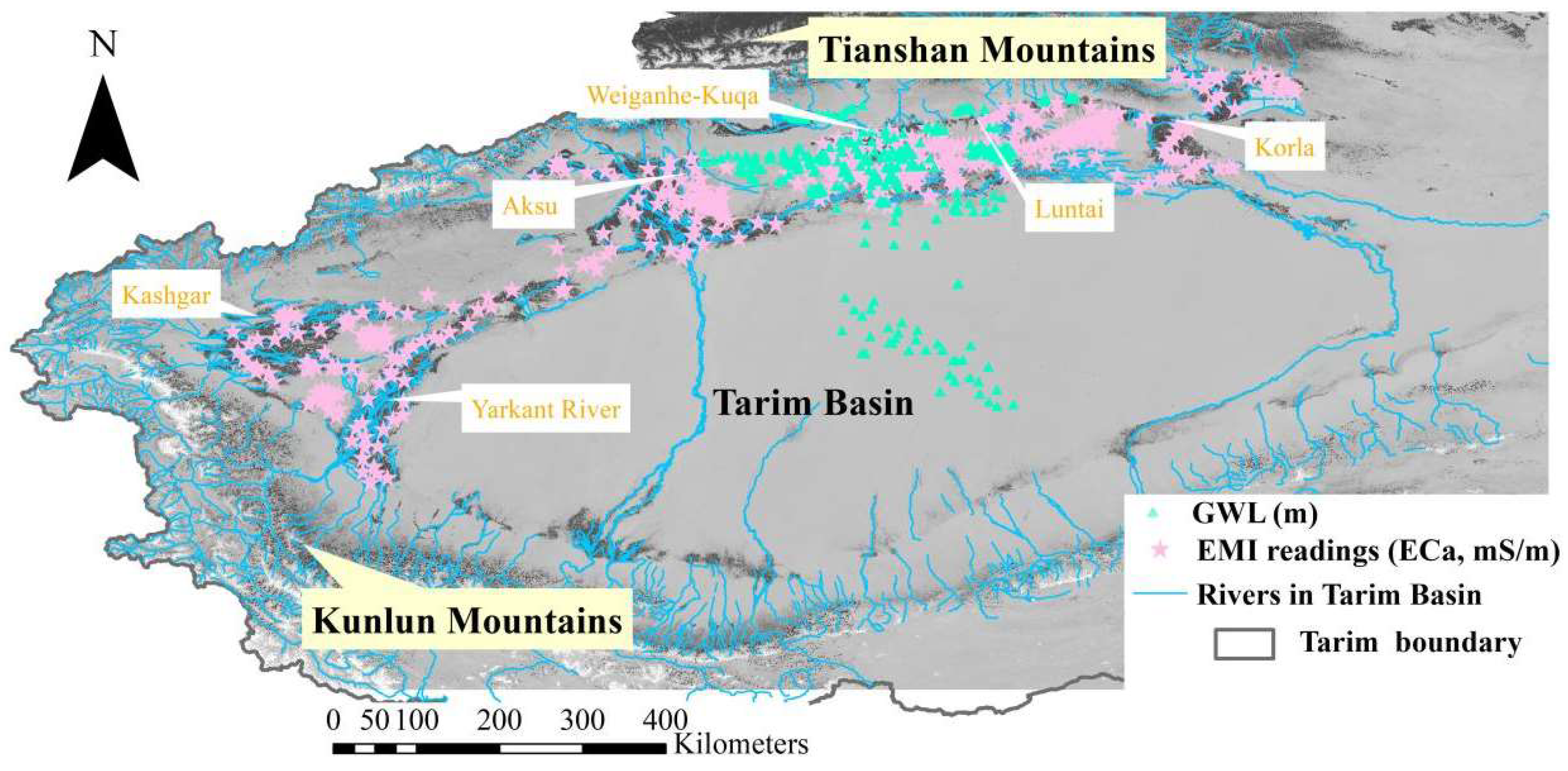
2.1. Study Area

The Tarim Basin, located in the southern part of Xinjiang (as illustrated in Figure 1), is characterized by its arid climate, which features minimal rainfall and high evaporation rates—key indicators of a distinct continental climate regime [35]. The region typically receives less than 50 mm of annual precipitation, in stark contrast to evaporation rates that range from 2300 to 3000 mm [39]. It benefits from abundant sunlight, with annual solar exposure between 2800 and 3100 h. The mean annual temperature ranges from 10 to 11 °C, while the cumulative temperature exceeding 10 °C reaches a substantial 4000 to 4350 °C. The prevalent soil types in this region include salinized Meadow soil, Poplar soil, saline soil, Oasis Alluvial soil, Aeolian sandy soil, and Marsh soil, collectively creating a diverse substrate for local ecology. The topography of the Tarim Basin slopes from higher elevations in the west to lower elevations in the east, with altitudes varying from 779 to 1031 m above sea level; the basin’s lowest point is at Lake Taitmar.

The Tarim River, meandering through the region, is recognized as China’s largest inland river system, encompassing a collective term for 114 rivers that are part of nine major hydrological networks, including the Aksu, Hotan, Yarkant, Chelchen, Keriya, Di, Kashgar, Kaidu-Kongqu, and Weigan rivers. These rivers are primarily fed by glacial meltwater [40]. Both groundwater and surface water in the study area flow together from west to east, exhibiting a general hydraulic gradient of 0.0002, which indicates a gentle and slow movement of water [41].

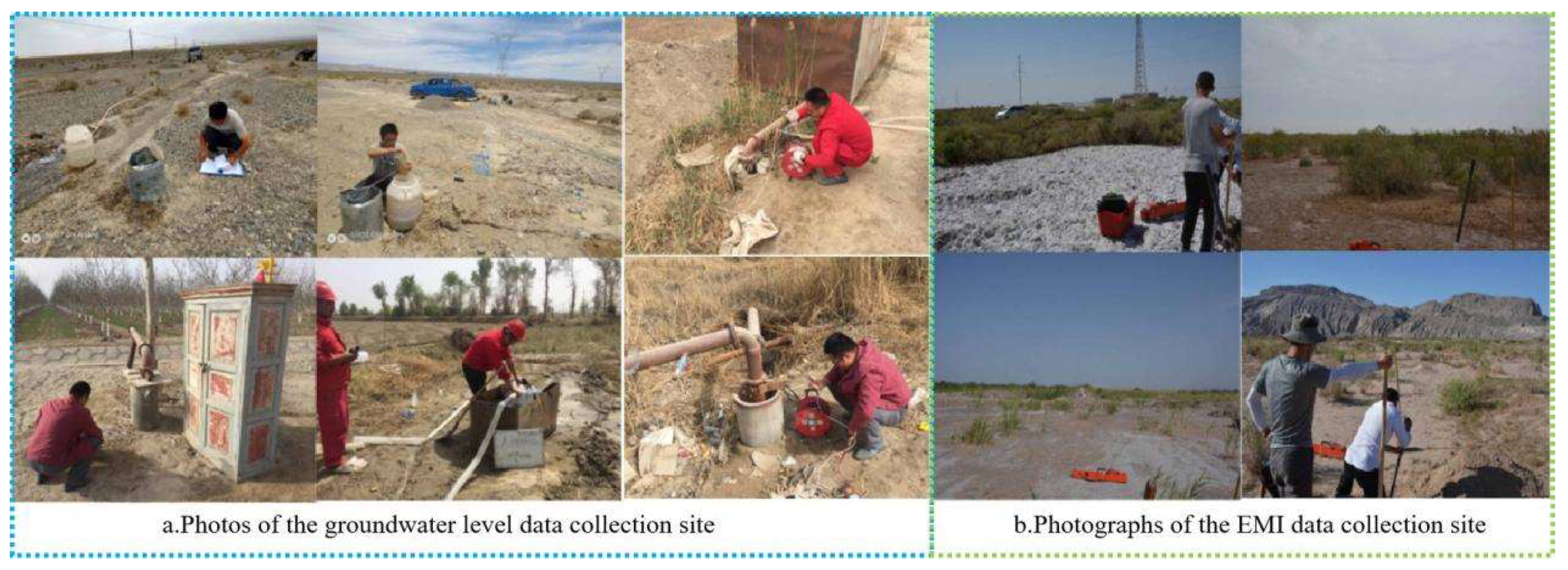
2.2. Field Measurements

Groundwater level observation data were obtained from the environmental surveillance and assessment initiative conducted during the pre-development phase of the oilfield. The sampling sites represented a diverse array of landscapes, including pre-mountain flood fans, irrigated agricultural areas, oasis–desert transition zones, and the desert itself. Groundwater samples were collected using a combination of mechanically drilled wells and pre-existing observation wells, as illustrated in Figure 2. Data collection occurred from April to June 2018, resulting in a comprehensive dataset comprising 436 groundwater level measurements (Figure 1)

Sample collection (ECa) was completed during two field surveys in the summers of 2018 and 2019. Sampling points were determined using a conditioned Latin hypercube sampling (cLHS) design. A range of environmental covariates were incorporated into the sampling design, including remote-sensing-derived variables (e.g., NDVI, ENDVI, and SSI: B4/B5), topographic variables (e.g., elevation from DEM and its derivatives like TWI, MRVBF, MRRTF, valley depth, and vertical distance to river networks), and land use and landform variables. Sampling point accessibility, indicated by road networks, was considered in the design and dynamically adjusted based on real-time road condition assessments to enhance sampling efficiency. Some desert areas were hard to reach, so samples were collected only from the edges of this landscape type. The research team, with extensive experience in the Kuche Oasis and familiarity with the local environment and roads, conducted the first sampling in 2018 based on preset points. To ensure comprehensiveness and address potential gaps in sampling other typical landscapes, supplementary sampling was carried out in the Kuche Oasis in 2019.

After post-processing, a total of 474 valid samples were obtained (Figure 1).

The EM38-MK2 instrument (EM38, Geonics Limited, Mississauga, ON, Canada) is equipped with two receiver coils, positioned 1 m and 0.5 m from the transmitter. When configured in the vertical dipole orientation, these coils measure to effective depths of 1.5 m and 0.75 m, respectively. In contrast, when set in the horizontal dipole configuration, they measure to effective depths of 0.75 m and 0.375 m. For this study, the vertical mode of the EM38-MK2 was utilized, allowing for a detection depth of 1.50 m. The survey employed a nonlinear sampling trajectory within a 90 m × 90 m quadrat. Before conducting the EMI measurements, surface temperatures were recorded to account for their influence on the raw EMI values, following the methodology outlined by Tromp et al. [42]. The temperature-corrected raw data underwent preliminary scrutiny to eliminate any zero or negative readings. The data collected from these nonlinear transects were then harmonized to uniformly reflect the apparent conductivity (ECa, mS/m) observed across the 90 m × 90 m sampling area at each site.

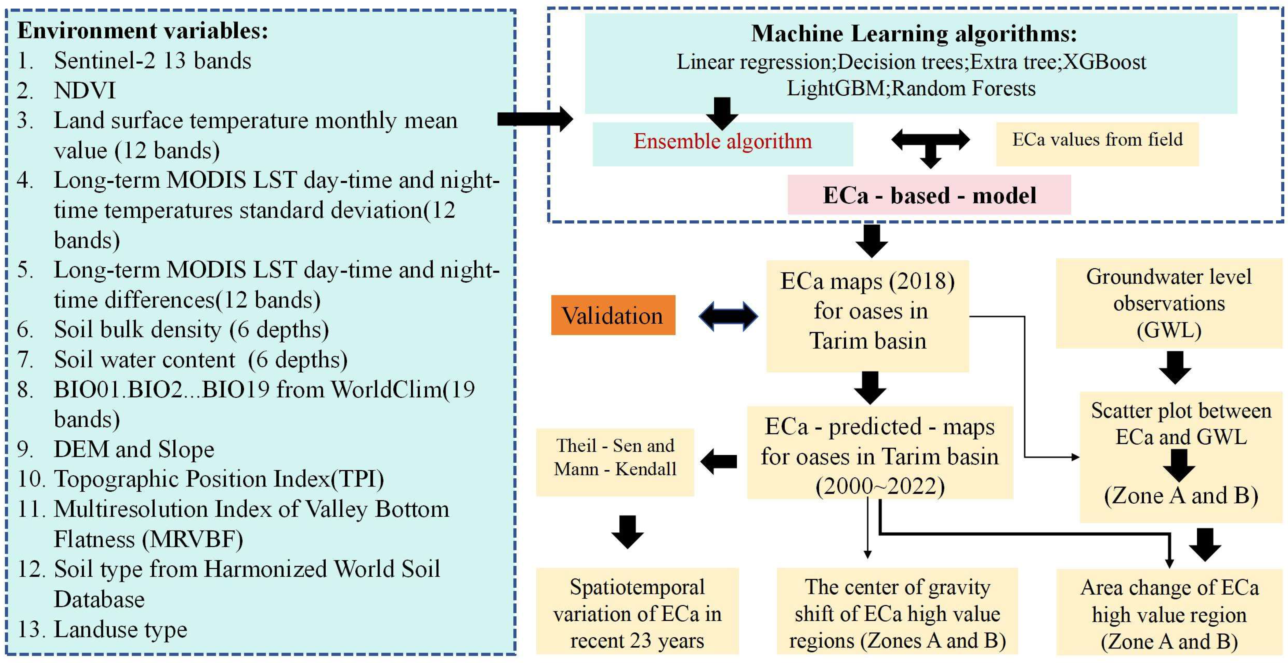
2.3. Environmental Variables

The optical data essential to this study were obtained from Sentinel-2 (2016–2022) and Landsat (2000–2022), an advanced satellite-based platform: https://earthengine.google.com (accessed on 8 February 2024). These datasets comprise multiple spectral bands, each of which underwent a thorough atmospheric correction and de-clouding process to ensure data integrity. The reason for using two data sources was to minimize the objective facts of cloud coverage and missing data.

Vegetation index (CSRI, EEVI, and GDVI) and soil index (SIT), which serve as vital indicators of soil moisture and groundwater availability [43,44], were calculated for the years 2016 to 2022. For each year, the median value (data from April to June) was determined to provide a robust annual representative measure.

Temperature, known to indirectly influence soil moisture [45,46], was incorporated using a suite of temperature products from the Openlandmap family, accessible via the Google Earth Engine (GEE) platform. The temperature data included the daytime monthly mean Land Surface Temperature (2000–2022), as well as the standard deviation of long-term Moderate-resolution Imaging Spectroradiometer (MODIS) Land Surface Temperature (LST) daytime and nighttime temperatures. Additionally, the study considered the long-term differences between daytime and nighttime MODIS LST at a 1 km resolution, based on the 2000–2022 time series. Each product consists of 12 bands, corresponding to the 12 calendar months, resulting in a comprehensive set of 36 environmental variables across the three datasets.

Soil bulk density, a critical physical property of soil, was utilized to assess the soil’s capacity to retain moisture [47]. This study employed Soil Bulk Density data from the OpenLandMap series (from GEE), which provides readings at six standard depths (0, 10, 30, 60, 100, and 200 cm) with a resolution of 250 m. Concurrently, Soil Water Content data from the same series, representing volumetric percentages at 33 kPa and 1500 kPa suctions for the same depths, were also utilized at a 250 m resolution.

Climate data were derived from 19 bioclimatic variables provided by WorldClim (BIO01 through BIO19) [48]. Detailed information is available at the following website: https://www.worldclim.org/data/bioclim.html (accessed on 15 October 2024). Additional datasets included solar radiation, saturated water pressure, and wind speed, with each dataset comprising 12 monthly bands.

The DEM-derived topographic variables indicated movement direction of the parent material and water, which indirectly suggested the location of accumulated soil salts. The fluctuations in topography directly affected the surface and underground runoffs. Slope, Topographic Position Index (TPI), and Multiresolution Index of Valley Bottom Flatness (MRVBF) were calculated using a digital elevation model within the System for Automated Geoscientific Analyses (SAGA, version 7.9.0). These indices are used to indicate low-lying areas.

This study also considered soil type and land use practices. Soil type data were sourced from the Harmonized World Soil Database v2.0, a comprehensive global soil inventory that provides detailed insights into soil properties, including morphology, chemistry, and physical characteristics, with a focus on 1 km resolution. This database is an invaluable resource for research in agriculture, food security, and climate change impacts. This study acknowledged that hydrothermal conditions under different land use patterns significantly affect soil quality and water and salt transport [49]. Therefore, global 30 m surface land use/cover products were selected [50] and obtained from the Finer Resolution Observation and Monitoring site at http://data.ess.tsinghua.edu.cn/ (accessed on 20 August 2024). This product includes seven land use types: arable land, grassland, shrubland, desert, unused land, urban areas, and water bodies. All variables were normalized between participating in model training.

2.4. Machine Learning

Linear regression is one of the simplest and most widely used algorithms in the machine learning toolbox. This statistical technique is employed for predictive analysis, establishing a linear relationship between a dependent variable (y) and one or more independent variables (x), hence the name linear regression.

Decision trees are a class of supervised machine learning algorithms that classify or predict data by navigating a series of true or false questions, which leads to a decision path [51]. Visually, they resemble tree structures, comprising various types of nodes: root, internal, and leaf. The root node signifies the beginning of the decision-making process, which then splits into internal nodes and concludes with leaf nodes. These leaf nodes indicate the final classification bins or numerical values. Renowned for their interpretability and ease of understanding, decision trees provide a transparent approach to data analysis.

The Extra Trees algorithm, similar to the Random Forest technique, generates numerous decision trees, each based on a unique dataset created through random sampling without replacement [6]. This method results in a diverse collection of trees, each with a randomly selected subset of features from the overall pool. A distinctive characteristic of Extra Trees is the random selection of a splitting value for each feature, in contrast to the traditional calculation of locally optimal values using metrics such as Gini or entropy. This randomness promotes a diverse and uncorrelated forest of trees.

The XGBoost algorithm, introduced by Chen and Guestrin [52], represents an advancement of the gradient boosting decision tree, utilizing a greedy algorithm alongside an approximation method to enhance the tree model. During tree construction, XGBoost begins by calculating the residuals—the differences between actual and predicted values. The true values are predetermined, while the predicted values are dynamically generated by the XGBoost algorithm as it optimally navigates the data samples. The algorithm evaluates the similarity scores of each root node and its descendant leaf nodes based on the residuals of potential splits, employing the gain—the difference between the sum of the leaf nodes’ similarities and the root node’s similarity—to determine the optimal split point. This iterative process shapes the model tree, with XGBoost being praised for its computational efficiency, flexibility, accuracy, and suitability for parallel processing, establishing it as a standard in geographic information mining and image pattern recognition.

LightGBM, an efficient gradient boosting decision tree algorithm developed by Microsoft [53], enhances the traditional GBDT and serves as a boosting-based ensemble learning algorithm. It addresses the scalability and speed limitations of conventional boosting algorithms, providing a solution that significantly reduces training time without sacrificing predictive accuracy and minimizing memory usage. LightGBM employs two primary strategies to accelerate training: Gradient-based One-Side Sampling (GOSS), which selects samples with significant gradients to enhance computational efficiency, and Exclusive Feature Bundling (EFB), which reduces data dimensionality by consolidating specific features.

The Random Forest (RF) algorithm, proposed by Breiman [54], is an ensemble learning method based on bagging, utilizing decision trees as its base learners within the bagging framework. It operates by drawing random samples with replacement from the training set, constructing a decision tree for each subset of samples, and combining the predictions from all trees through averaging. The CART algorithm plays a crucial role in generating regression decision trees; it is a binary tree that partitions the dataset based on the most effective feature, determined by minimizing the Mean Squared Error (MSE). This process is iteratively applied until all data points are exhausted or the MSE falls below a predefined threshold. RF has become a preferred solution in the field of remote sensing information extraction due to its effectiveness.

An ensemble model is a composite structure formed by individual models, with their predictions amalgamated through weighted averaging or voting. The primary strategies for creating ensembles include bagging, exemplified by Random Forest, and boosting, as demonstrated by XGBoost. These methods integrate outputs from multiple instances of the same algorithm. Advanced techniques, such as those described in “Ensemble Selection from Libraries of Models” [55], combine diverse models to construct an ensemble. The process entails (1) incrementally adding the model from the library that maximizes the ensemble’s performance on a validation set; (2) repeating this step for a predefined number of iterations or until all models have been included; and (3) selecting the ensemble from the nested set that exhibits optimal performance on the validation set. All algorithms were executed in ARCGIS pro 3.0.

2.5. Theil–Sen and Mann–Kendall

The Theil–Sen method is a non-parametric statistical approach for trend estimation, well-suited for trend analysis of long-term time series data. The beta (β) represents the annual change trend in ECa; if β > 0, the sample data exhibit an increasing trend, whereas if β < 0, the sample data demonstrate a decreasing trend. The Mann–Kendall trend test is also a non-parametric statistical method often used in conjunction with the aforementioned Theil–Sen slope method for analyzing samples, and it is frequently applied to assess the trends in long-term time series data in meteorology, hydrology, and other fields [56,57]. The categories of Mann–Kendall test trends are shown in

Table 1. Interpretation of the Mann–Kendall trend test results.

β	Z	Interpretation of the Temperature Trend
Β > 0	Z > 2.58	Increasing Trend significant at 99% confidence level
	1.96 < Z ≤ 2.58	Increasing Trend significant at 95% confidence level
	1.65 < Z ≤ 1.96	Increasing Trend significant at 90% confidence level
	0 < Z ≤ 1.65	Increasing Trend not significant
Β = 0	0	No Trend
Β < 0	0 > Z ≥ −1.65	Decreasing Trend not significant
	−1.65 > Z ≥ −1.96	Decreasing Trend significant at 90% confidence level
	−1.96 > Z ≥ −2.58	Decreasing Trend significant at 95% confidence level
	Z < −2.58	Decreasing Trend significant at 99% confidence level

. In this study, we employ this method to conduct a significance test analysis of the trend in groundwater storage changes in the study area, calculating the significance Z-value for each pixel at a grid level and performing a test at a 95% confidence level (α = 0.05). The calculation formula for the Z-value is as follows:

$$S={\displaystyle {\sum }_{i=1}^{n=1}{\displaystyle {\sum }_{j=i+1}^{n}Sgn(X_j=X_{i=1})}}$$

(1)

$$Sgn(X_{\mathrm{j}}-X_i)=\left(\begin{array}{l}1, X_j-X_i>0\\ -1, X_j-X_i=0\\ -1, X_j-X_i<0\end{array}\right)$$

(2)

$$V\mathrm{ari}(S)={\displaystyle \frac{n(n+1)(2n+5)}{18}}$$

(3)

$$Z=\left(\begin{array}{l}{\displaystyle \frac{S-1}{\sqrt{V\mathrm{ari}(S)}}}, S>0\\ 0,S=0\\ {\displaystyle \frac{S-1}{\sqrt{V\mathrm{ari}(S)}}}, S<0\end{array}\right)$$

(4)

In the formula, n represents the number of samples; S denotes the statistical quantity of the Mann–Kendall trend test, which is normally distributed; and Var(S) is the variance of S.

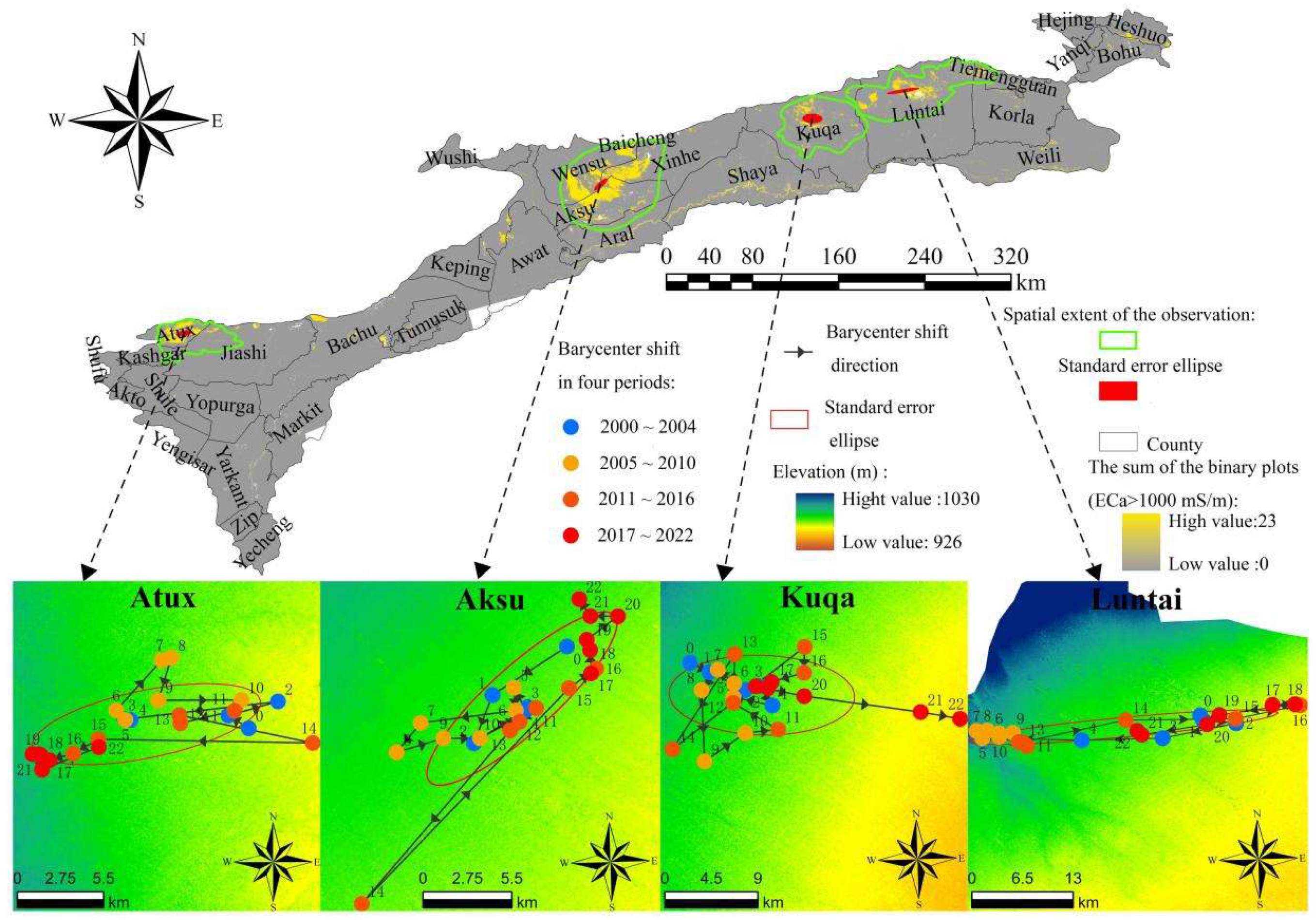
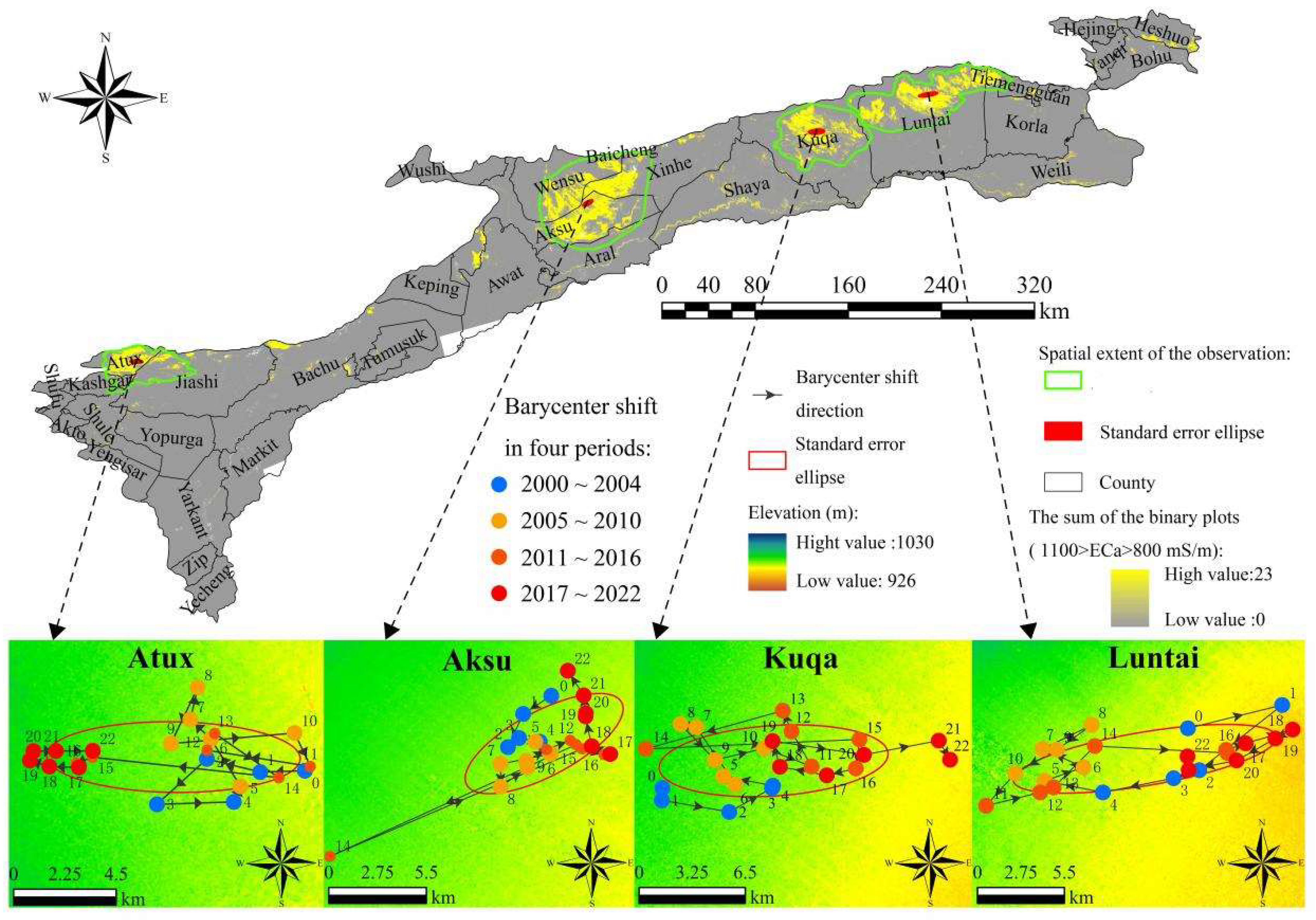
2.6. Barycenter Shift

The convergence and dispersion of various substances and energy in space, at a given moment, will culminate in a center of mass. The direction, velocity, and intensity of the barycenter shift are the most effective indicators to characterize the spatial variation of a particular substance [58]. The barycenter shift of ECa is a crucial aspect of studying the spatial pattern changes of water and salt, capable of indirectly reflecting the processes and trends of the spatiotemporal evolution of water resources and unveiling the characteristics of their dynamic fluctuations. Consequently, this study employs the gravity center method, frequently utilized in geography and economics, to calculate the ECa center of mass for the study area in the years 2000 and 2022. The position of the center of mass is denoted by geographical coordinates, with the expression formula as follows:

$$\{\begin{array}{l}\overline{X}={\displaystyle \frac{{\displaystyle {\sum }_{\mathrm{i}=1^n}{X}_{i}EC{\mathrm{a}}_i}}{{\displaystyle {\sum }_{\mathrm{i}=1^n}EC{a}_i}}}\\ \overline{Y}={\displaystyle \frac{{\displaystyle {\sum }_{\mathrm{i}=1^n}{Y}_{i}EC{\mathrm{a}}_i}}{{\displaystyle {\sum }_{\mathrm{i}=1^n}EC{a}_i}}}\end{array}$$

(5)

$\overline{X}$, $\overline{Y}$ represent the barycenter; X_i, Y_i represent the latitude and longitude coordinates of the i-th point; and ECa_i denotes the ECa value of the i-th point.

2.7. Flowchart

Please see Figure 3 for the specific flow:

2.8. Validation

The whole dataset (474 samples) was randomly split into calibration (334 samples) and validation (140 samples) sets at a ratio of 70% to 30% with 100 repeats. The R² and RMSE were used to evaluate ECa model accuracy on the validation set. Higher R² and a lower RMSE close to 0 mean better model accuracy.

$$R^2=1-{\displaystyle \frac{\sqrt{{\displaystyle \sum _i^{\mathrm{n}}{(\stackrel{\Delta }{y_i}-y_i)}^2}}}{\sqrt{{\displaystyle \sum _i^{\mathrm{n}}{(y_i-{\overline{y}}_i)}^2}}}}$$

(6)

$$RMSE=\sqrt{{\displaystyle \frac{{\displaystyle \sum _i^{\mathrm{n}}{(\stackrel{\Delta }{y_i}-y_i)}^2}}{n}}}$$

(7)

where y_i and $\stackrel{\Delta }{y_i}$ are observation and prediction for sample i, $\overline{y}$ is the mean of all the observations, and n is the number of samples.

3. Results

3.1. Statistical Characterization of GWL and ECa

This study conducted a comprehensive statistical analysis to characterize the distribution of ground observation data (

Table 2. Distributional characteristics of ground observation data.

Observed Object	Minimum	Maximum	Mean	Median	Std. Deviation	Coefficient of Variation
ECa (mS/m)	1.39	1764.00	356.00	198.80	378.80	106.40%
GWL (m)	0.79	150.30	11.28	5.98	21.07	186.71%

). The findings indicated that the electrical conductivity of the soil (ECa) exhibited a wide range, with the highest and lowest recorded values reaching 1764 mS/m and 1.39 mS/m, respectively. The groundwater level (GWL) observations had an average of 11.28 m, but they encompass a broad range from a maximum of 150.30 m to a minimum of 0.79 m. The coefficients of variation for these parameters exceed the 100% threshold, with 106.40% for ECa and an even more pronounced 186.71% for GWL. These significant coefficients highlighted the markedly uneven spatial distribution of the observed parameters, emphasizing the complexity of the hydrogeological conditions within the study area [30,59].

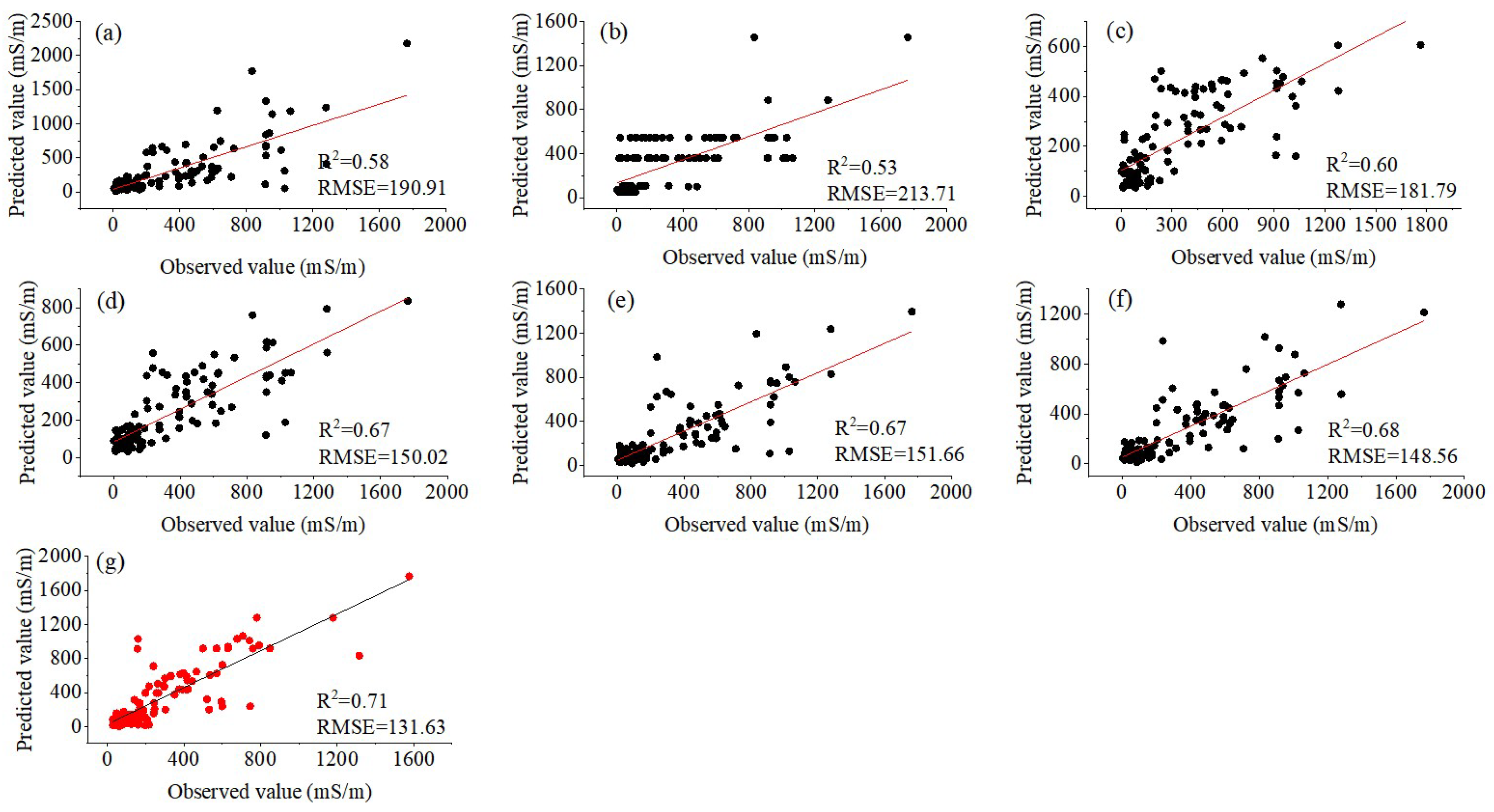
3.2. Validation of Apparent Conductivity Modeling

The modeling of electrical conductivity (ECa) was rigorously validated using machine learning algorithms, with a holdout set consisting of 30% of the samples reserved for this purpose. A suite of seven learning algorithms, including both individual and ensemble methods, was meticulously selected to identify the most suitable algorithm for ECa modeling. As illustrated in Figure 4, the ensemble algorithm emerged as the most effective, achieving the highest coefficient of determination (R²) at 0.71. In contrast, the Decision Tree algorithm performed the least well, with the lowest R² value of 0.53. The Random Forest, XGBoost, and LightGBM algorithms demonstrated closely competitive performance, with R² values of 0.67, 0.67, and 0.68, respectively. These results emphasized the relative effectiveness of ensemble methods in capturing the complexities of ECa modeling while highlighting the variability in performance across different machine learning approaches.

This study utilized an ensemble algorithm to comprehensively map the soil electrical conductivity (ECa) in the Tarim Basin. As illustrated in Figure 5, areas with heightened ECa values were primarily located in the Kashgar Oasis, Aksu Oasis, Kuqa-Luntai Oasis, and Ruoqiang Oasis, each exhibiting distinct characteristics. Notably, the eastern side of the Aksu Oasis showed the highest ECa readings. The predicted distribution of ECa grades reveals a nuanced spatial pattern: the 0–400 mS/m range is predominantly associated with farmland and desert within the irrigated zones. The pixel value of ECa in the range of 400 to 600 mS/m is mainly distributed in the periphery of oasis irrigation areas and on both sides of the river bank. The 800–1000 mS/m area was more concentrated, typically found in the salt accumulation zones beyond the smaller oases. Lastly, regions exceeding 1000 mS/m were mainly concentrated in the Aksu Oasis, indicated significant salt accumulation in this area.

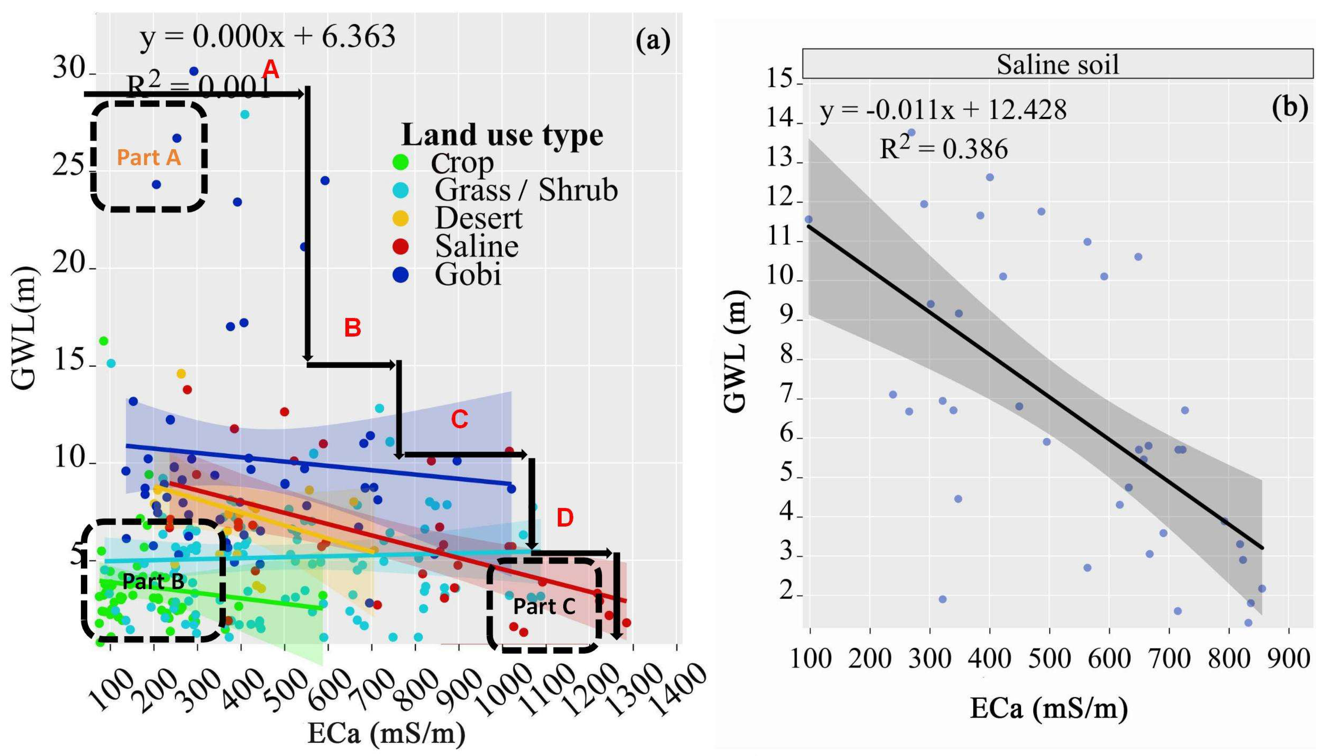
3.3. Relationship Between GWL and ECa

This study examined the correlation between predicted soil conductivity (ECa) and groundwater level (GWL) by constructing two-dimensional scatterplots to visualize their relationship. As illustrated in Figure 6, the feature space did not reveal a discernible linear correlation between ECa and GWL. However, an intriguing pattern emerged: as ECa values increased, the distribution of GWL became concentrated into four distinct intervals: 0–600 mS/m corresponds to a GWL range of 0–31 m, 600–800 mS/m corresponds to a range of 0–15 m, 800–1100 mS/m corresponds to a range of 0–10 m, and values exceeding 1100 mS/m are found within the 0–5 m region. To gain further insights, this study classified sample points within the feature space based on their land use classification. Notably, a more pronounced linear relationship was observed exclusively in saline areas, with an R² value of 0.38 and a significant p-value of less than 0.01. In contrast, other land use types exhibited weak or no correlation, indicating complex interactions among ECa, GWL, and land use that extend beyond simple linear associations. This nuanced analysis underscores the complexity of hydrogeological interactions and emphasizes the necessity for a more sophisticated approach to understanding these dynamics, particularly in the context of agricultural planning initiatives.

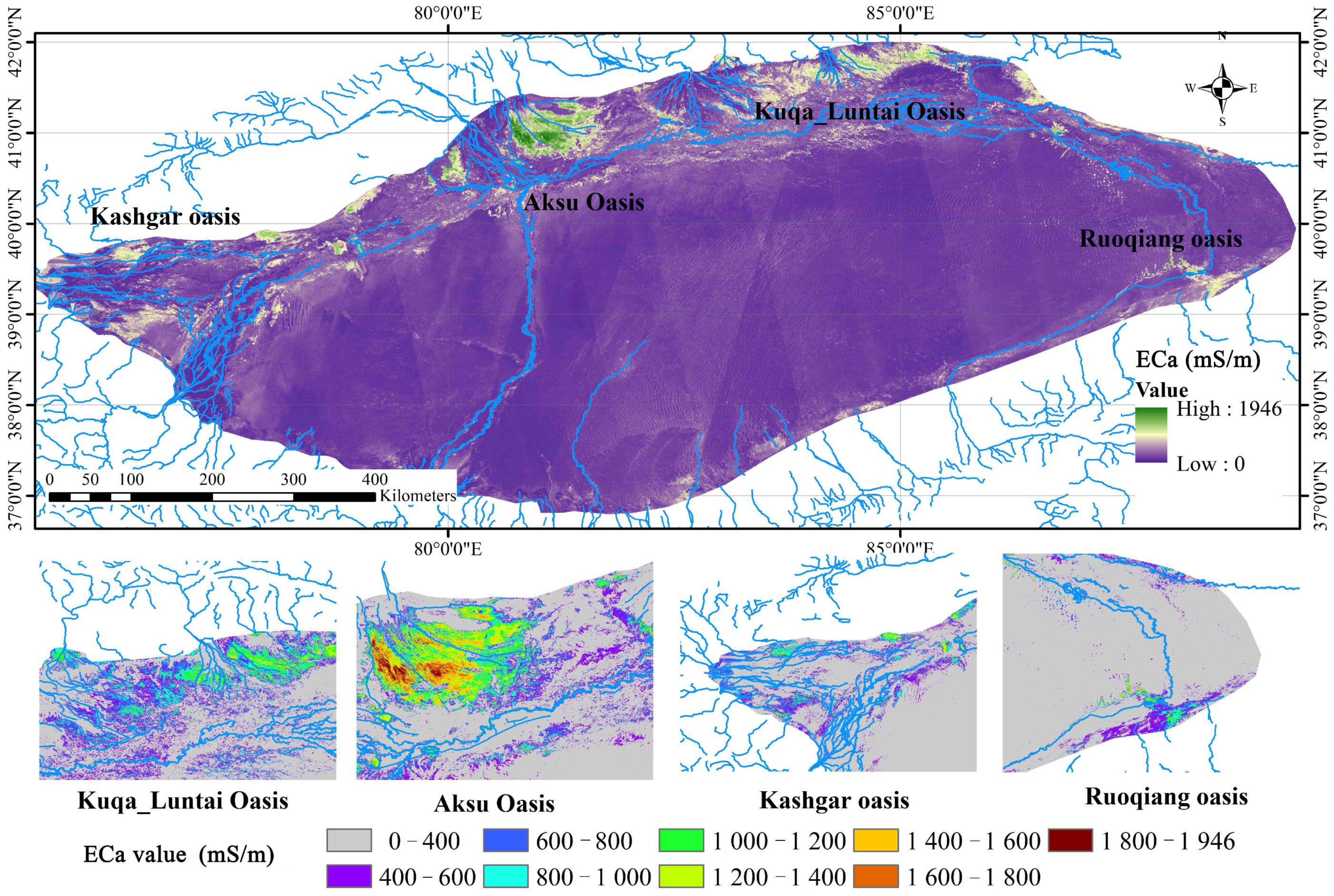
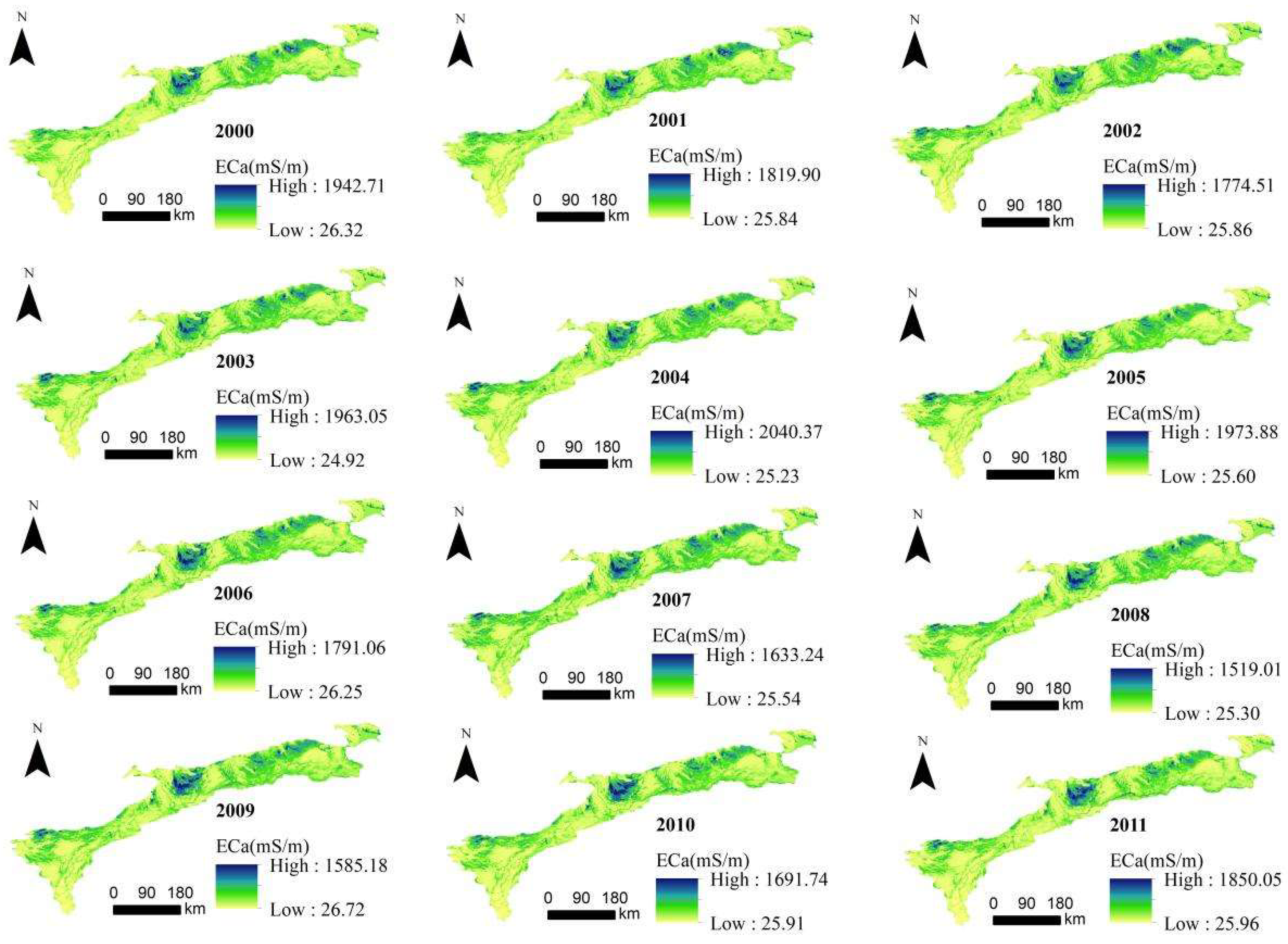
3.4. Temporal and Spatial Distribution Characteristics of ECa

Based on the ensemble model, annual ECa spatial distribution maps were generated for the years 2000 to 2022 (Figure 7 and Figure 8). The distribution patterns observed for 2018 and 2019 closely resemble those predicted by Wang et al. [59]. Upon comparison, it was found that high-value areas (ECa > 1100 mS/m) were predominantly located in the southern part of Luntai, as well as in the eastern and western regions of the Weigan–Kuqa River oasis, the desert area north of the Alar River, the oasis–desert belt along both banks of the lower reaches of the Yeerqiang River, and the alluvial fan plain area near the tail lake south of the Wudaoban Railway Station. In contrast, low-value areas are primarily found in natural oases, artificial oases, and desert regions.

Further statistical analysis indicated that the extent of the high ECa value zone (ECa > 1100 mS/m, designated as Zone A) has experienced periodic fluctuations from 2000 to 2022 (Figure 9). The area of the region reached its peak in the years 2004, 2011, and 2017, each characterized by a maximum in values. In contrast, the lowest points occurred in 2001, 2008, 2014, and 2022, during which the area is at its minimum. The trend of area for Zone B (800 mS/m < ECa ≤ 1100 mS/m) mirrored this pattern. Over the 23-year span, the distribution area of Zone B exhibited a declining trend, with a correlation coefficient (r) of −0.40, suggesting a modest but consistent decrease. However, the area of the high-value region (Zone A) had not undergone significant changes. This study suggested that these patterns may be linked to cyclical variations in water supply, implying a connection between hydrological cycles and the spatial distribution of soil salinity [60,61,62].

The Theil–Sen and Mann–Kendall trend tests were employed to analyze the spatial variation characteristics of ECa in the study area from 2000 to 2022 (Figure 10). ECa values exhibited a significant increase in the desert transition zone between the Aksu Oasis and the Weigan River–Kuqa River Oasis, the desert zone surrounding the Huanluntai Oasis, and the desert transition zone along both banks of the lower reaches of the Yeerqiang River. Conversely, ECa decreased in both oasis and desert regions. The statistical results indicated that ECa increased in 10% of the area, with 5.43% showing a significant increase; ECa decreased in 53% of the area, of which 42.67% experienced a significant decrease; ECa remained unchanged in 36.89% of the area. The study binarized the areas of Zone A and Zone B into two categories (0 and 1) for each year, which were then summed to analyze their spatial changes over the past two decades (Figure 11 and Figure 12). The distribution area of Zone A coincided with the region of significant increases in ECa value during this period. Additionally, the buffer zones along the banks of the Aksu and Tarim Rivers served as the primary distribution areas for high ECa values. Zone B, while similar to Zone A, had a larger distribution area and was predominantly situated in the desert transition zone to the east of the Aksu Oasis. Subsequently, this study mapped the annual migration changes of the barycenter in the four high-value zones, which represent the main storage areas for salt drainage from the irrigation regions within the oasis.

Over the past 23 years, the trajectory of the barycenter shift in Zone A indicated that the Atux, Aksu, Kuqa, and Luntai areas have exhibited orientations of east–west, northeast–southwest, east–west, and east–west (Figure 11), respectively. In terms of the distance of the barycenter shift, the Luntai area showed the largest value at 24 km, followed by Kuqa at 23 km, Aksu at 19 km, and Atux at 13 km. The situation in Zone B was similar to that in Zone A. The trajectory of the barycenter shift in Zone B for the Atux, Aksu, Kuqa, and Luntai areas was also oriented in east–west, northeast–southwest, east–west, and east–west directions, respectively (Figure 12). Regarding the distance of the barycenter shift, the Luntai area again showed the largest value at 42 km, followed by Kuqa at 27 km, Aksu at 23 km, and Atux at 17 km. These results demonstrated that the impact of groundwater resources on Zone B was greater than that on Zone A, indicating that the area and spatial changes of groundwater levels below 5 m are more sensitive to water resource supply.

4. Discussion

The Xinjiang plains region is a vital grain production and food security stronghold for China, with over 90% of its groundwater extraction allocated to irrigated agriculture. In response to global climate warming, the Xinjiang area has experienced a warming and humidifying trend over the past 40 years, accompanied by an accelerated rate of glacier melt [19], which has significantly affected the regional water cycle. Based on findings from three groundwater resource surveys and assessments conducted by the water conservancy sector, it has been established that the volume of groundwater resources in the Xinjiang plains showed a decreasing trend from 1956 to 2016 [63]. In this context, the present study utilized remote sensing and electromagnetic induction techniques to analyze the spatiotemporal dynamics of ECa.

4.1. ECa High Values Are Indicators of Shallow Groundwater (GWL < 5 m)

This study represented a pioneering effort to analyze the relationship between electrical conductivity (ECa) and GWL. It revealed that the EM38 instrument was particularly effective at identifying areas where the groundwater level (GWL) was less than 5 m. As the depth of the groundwater table decreases, the impact of water and salt on EMI measurement values becomes more pronounced compared to other environmental factors, a phenomenon attributed to the inherent characteristics of EMI’s electromagnetic induction [14,16]. The research indicated that regions with high ECa values (ECa > 1100 mS/m) were predominantly located in the Aksu Oasis desert ecological region. The long-term presence of shallow groundwater in this area led to elevated moisture and salt content in the soil (designated as Part C in the two-dimensional feature space of Figure 6). In contrast, when the soil exhibited higher moisture content but relatively lower salt levels, as observed in farmlands (Part B), the ECa measurement values tended to be lower.

Additionally, areas with similar ECa values may correspond to the relatively high-altitude Gobi region, where the groundwater table is deeper. This region primarily relies on precipitation for soil moisture replenishment and typically exhibits lower salt content (identified as Part A in the two-dimensional feature space of Figure 6a). The variation in ECa values in other regions of the feature space (among Part A, D, and C) is influenced by a nonlinear combination of environmental factors, including water, salt, and soil texture.

Furthermore, the observed stepped relationship between ECa and GWL, along with the randomness exhibited by the scatter points within each interval, may be attributed to errors in the predicted ECa values. Notably, the maximum R² value for ECa fitting accuracy depicted in Figure 4 was 0.71, indicating that 29% of spatial variability remains unexplained. However, the predicted and observed values for the high-value areas (ECa > 1100 mS/m) were relatively close, suggesting that the areas inferred from ECa to have GWL < 5 m were credible.

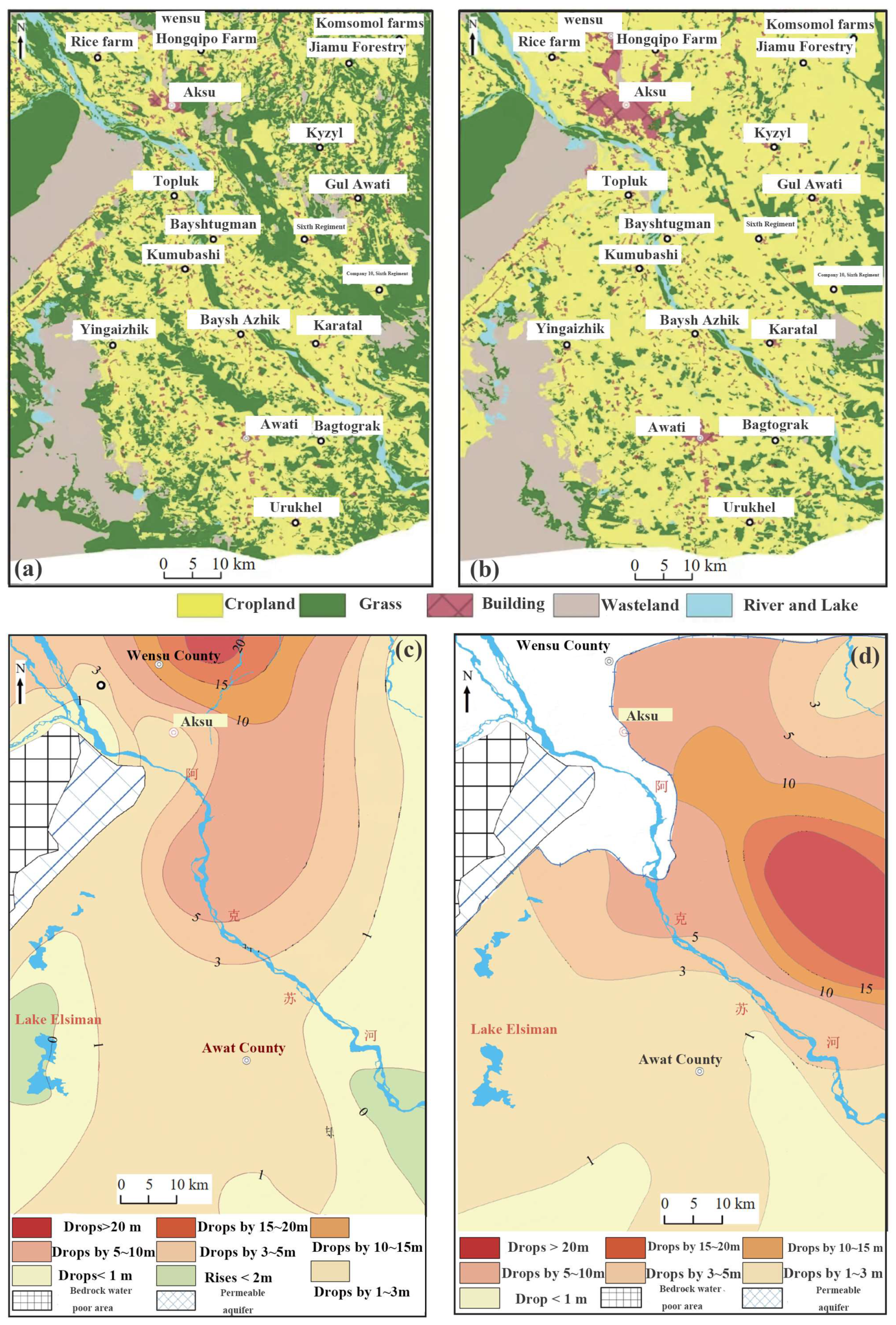
4.2. Land Use and Climate Change Are the Main Reasons for ECa Trends

Trend analysis indicated that areas exhibiting increasing ECa values were predominantly situated in desert regions, particularly between the Aksu Oasis and the Kuqa Oasis. From 2000 to 2018, the total mass loss of glaciers in the Aksu Basin amounted to 0.56 ± 0.09 Gt [64]. The loss of glaciers has contributed to an increase in the runoff of the Aksu River, which is also linked to rising temperatures in the glacier-rich Sary-Jaz River basin and the subsequent acceleration of glacier melting [65]. Spatiotemporal analysis of surface temperature changes in Xinjiang from 2000 to 2020 revealed a warming trend of 0.24 °C per decade, with 87.20% of the warming occurring in the Gobi Desert and regions with high levels of human activity [66]. Between 1960 and 2018, areas susceptible to drought shifted from the northwest to the southeast, with severe droughts predominantly affecting the central (Aksu region) and southern parts of the Tarim Basin [67]. Consequently, we hypothesized that the increase in temperature and runoff in this region had resulted in greater water and salt supply. Additionally, the expansion of farmland within the oasis led to a significant accumulation of soil salts in desert areas.

Over the past three decades (1992–2020), utilization of water resources for irrigation in Xinjiang has shown an upward trend [20], resulting in a marked decline in groundwater levels. The original saline-alkali grasslands (characterized by high ECa values) have gradually been transformed into farmland (characterized by low ECa values), further lowering the average ECa value in the region. Taking Aksu as a case study, the irrigated area doubled from approximately 4100 square kilometers in 1994 to about 8200 square kilometers in 2020 [68], with the most significant increase occurring between 2004 and 2009 [69]. An analysis of land use changes between 1979 and 2022 revealed a substantial conversion of grassland (and forest) areas into arable land [19]. The demand for irrigation water in Aksu has correspondingly risen, leading to varying degrees of decline in both shallow and confined water levels [68,70]. According to the fluctuation map of shallow groundwater levels from 1979 to 2022 [19], areas that experienced a decline in shallow water burial depth of 1–3 m represented a significant proportion (over 40%)(Figure 13). Concurrently, north of Kara Tal Town in the study area, the overall decline in confined water head ranged from 3 m to 20 m, while south of this area, the decline was less than 3 m and gradually decreased from north to south.

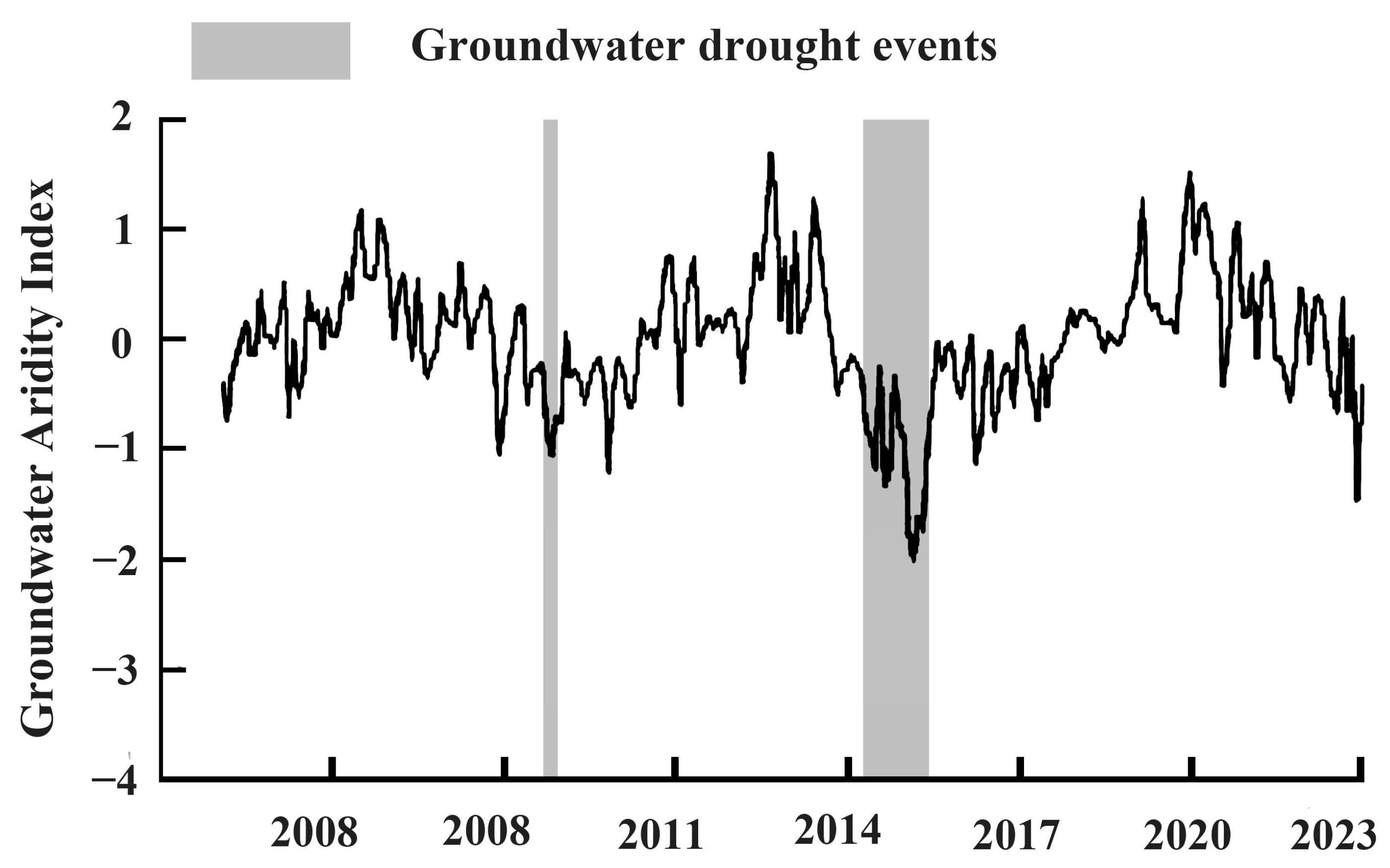
4.3. The Relationship Between Groundwater Resource Reserves and the Area Change of the ECa High Value Area

The research results of others are cited in this study to confirm the feasibility of the proposed method. Based on observations from the Gravity Recovery and Climate Experiment (GRACE), a groundwater drought index (GDI) was constructed to monitor drought conditions in areas with limited observational data, which was proposed by Zhao et al. (2017) [71]. This index was derived by standardizing the groundwater storage change time series for each grid in the Xinjiang plain area, as calculated from the water balance equation. The run theory, a widely used method for analyzing time series, was employed to identify drought events. According to this method, a groundwater drought index value of less than −0.5 indicates the occurrence of a groundwater drought event, with detailed calculations of its characteristic variables provided in the Wang et al. article [72] (Figure 14). This approach was used to analyze the temporal variation of the groundwater drought index in the Xinjiang plain area from 2003 to 2022 [71]. The results indicated that the southern Xinjiang plain experienced groundwater drought events lasting four months from September to December 2008 and 15 months from April 2014 to June 2015 [73]. Figure 9 and Figure 14 illustrate that the changes in the area of ECa in this study exhibit similarities to the variations in groundwater storage (indicated by GDI mean value). The research findings corresponded to relatively smaller areas in Zone A and B during the years 2001, 2008, 2014, and 2022. However, the GDI primarily depends on GRACE observation results, and the low spatial resolution of this dataset significantly limits its applicability in management. These findings demonstrated that high spatial resolution ECa data can provide detailed information and may serve as a vital supplement to GRACE.

To sum up, this study still needs to make efforts in the following directions. First, the sampling period of this study was summer of the year, and the prediction period was also concentrated in this period. Although the groundwater table in the study area has the same trend of rising and falling in different areas, it may change differently in other places due to geographical differences. Second, to understand how ECa has changed in the past for other seasons, it is recommended to build models for specific periods. In addition, we also need to emphasize the importance of sample selection in long-term monitoring, because the model built on this sample set should have the ability of spatial and temporal migration. Land use may change over a long period, and the sample should cover all types as much as possible.

5. Conclusions

While current long-term research predominantly focuses on land use transitions, fluctuations in crop varieties, dynamics of irrigation demand, and trends in temperature and precipitation, our understanding of the complex interplay between water and salt dynamics in the context of declining groundwater levels in this region remains limited. This limitation is largely due to the lack of hydrological monitoring stations and the scarcity of comprehensive field observation data, which are crucial for a more nuanced understanding of these environmental changes. In this study, we predicted the changes in electrical conductivity (ECa) over a long time series (2000–2022) based on the constructed model and analyzed the temporal and spatial characteristics of ECa changes. The following conclusions were drawn by comparing the results with the variations in groundwater resources:

1. The method was most effective in identifying areas where groundwater depth exceeded 5 m, particularly when the electrical conductivity (ECa) exceeded 1100 mS/m.

2. A spatiotemporal analysis from 2000 to 2022 revealed a significant reduction in ECa values within the artificial irrigation zones of the oasis clusters. In contrast, the desert–oasis transition zones in Atux, Aksu, Kuqa, and Luntai have experienced a notable increase in ECa.

3. The fluctuations in the areas designated as Zone A (where ECa > 1100 mS/m) and Zone B (where 1100 mS/m > ECa > 800 mS/m) were found to correlate with the cyclical changes observed in the GDI.

References

1. Scanlon, B.R.; Fakhreddine, S.; Rateb, A.; de Graaf, I.; Famiglietti, J.; Gleeson, T.; Grafton, R.Q.; Jobbagy, E.; Kebede, S.; Kolusu, S.R. Global water resources and the role of groundwater in a resilient water future. Nat. Rev. Earth Environ. 2023, 4, 87–101. [Google Scholar]
2. Singh, A. Soil salinization management for sustainable development: A review. J. Environ. Manag. 2021, 277, 111383. [Google Scholar]
3. Khorrami, M.; Malekmohammadi, B. Effects of excessive water extraction on groundwater ecosystem services: Vulnerability assessments using biophysical approaches. Sci. Total Environ. 2021, 799, 149304. [Google Scholar] [PubMed]
4. Wang, F.; Wei, Y.; Yang, S. Enhanced Understanding of Key Soil Properties in Northern Xinjiang Using Water-Heat-Spectral Datasets Based on Bioclimatic Guidelines. Land 2023, 12, 1769. [Google Scholar] [CrossRef]
5. Gao, J.; Li, Z.; Chen, Z.; Zhou, Y.; Liu, W.; Wang, L.; Zhou, J. Deterioration of groundwater quality along an increasing intensive land use pattern in a small catchment. Agric. Water Manag. 2021, 253, 106953. [Google Scholar]
6. Geurts, P.; Ernst, D.; Wehenkel, L. Extremely randomized trees. Mach. Learn. 2006, 63, 3–42. [Google Scholar]
7. Yin, X.; Feng, Q.; Li, Y.; Deo, R.C.; Liu, W.; Zhu, M.; Zheng, X.; Liu, R. An interplay of soil salinization and groundwater degradation threatening coexistence of oasis-desert ecosystems. Sci. Total Environ. 2022, 806, 150599. [Google Scholar] [CrossRef] [PubMed]
8. Li, X.; Long, D.; Scanlon, B.R.; Mann, M.E.; Li, X.; Tian, F.; Sun, Z.; Wang, G. Climate change threatens terrestrial water storage over the Tibetan Plateau. Nat. Clim. Change 2022, 12, 801–807. [Google Scholar]
9. Bogena, H.R.; Weuthen, A.; Huisman, J.A. Recent developments in wireless soil moisture sensing to support scientific research and agricultural management. Sensors 2022, 22, 9792. [Google Scholar] [CrossRef]
10. Brogi, C.; Huisman, J.; Pätzold, S.; Von Hebel, C.; Weihermüller, L.; Kaufmann, M.; Van Der Kruk, J.; Vereecken, H. Large-scale soil mapping using multi-configuration EMI and supervised image classification. Geoderma 2019, 335, 133–148. [Google Scholar]
11. Corwin, D.L.; Lesch, S.M. Protocols and guidelines for field-scale measurement of soil salinity distribution with ECa-directed soil sampling. J. Environ. Eng. Geophys. 2013, 18, 1–25. [Google Scholar]
12. Corwin, D.L.; Lesch, S.M. Validation of the ANOCOVA model for regional-scale ECa to ECe calibration. Soil. Use. Manag. 2016, 33, 178–190. [Google Scholar]
13. Doolittle, J.A.; Brevik, E.C. The use of electromagnetic induction techniques in soils studies. Geoderma 2014, 223, 33–45. [Google Scholar] [CrossRef]
14. McLachlan, P.; Schmutz, M.; Cavailhes, J.; Hubbard, S. Estimating grapevine-relevant physicochemical soil zones using apparent electrical conductivity and in-phase data from EMI methods. Geoderma 2022, 426, 116033. [Google Scholar]
15. Peralta, N.R.; Alesso, C.A.; Costa, J.L.; Martin, N.F. Mapping soil depth in southern pampas Argentina using ancillary data and statistical learning. Soil. Sci. Soc. Am. J. 2022, 86, 65–78. [Google Scholar]
16. Akramkhanov, A.; Brus, D.J.; Walvoort, D.J.J. Geostatistical monitoring of soil salinity in Uzbekistan by repeated EMI surveys. Geoderma 2014, 213, 600–607. [Google Scholar] [CrossRef]
17. Huang, J.; Koganti, T.; Santos, F.A.M.; Triantafilis, J. Mapping soil salinity and a fresh-water intrusion in three-dimensions using a quasi-3d joint-inversion of DUALEM-421S and EM34 data. Sci. Total Environ. 2017, 577, 395–404. [Google Scholar] [CrossRef]
18. Li, Y.; Chang, C.; Wang, Z.; Zhao, G. Remote sensing prediction and characteristic analysis of cultivated land salinization in different seasons and multiple soil layers in the coastal area. Int. J. Appl. Earth. Obs. 2022, 111, 102838. [Google Scholar] [CrossRef]
19. Wang, B.; Zhang, J.; Long, R.; Yu, K.; Jiang, J.; Yang, B.; Lu, Y. Evolution and Genetic Pattern of Groundwater Flow Field in the Aksu River Basin of Xinjiang Over the Past 40 Years. Northw. Geol. 2024, 57, 252–261. [Google Scholar]
20. Geng, Q.; Zhao, Y.; Sun, S.; He, X.; Wang, D.; Wu, D.; Tian, Z. Spatio-temporal changes and its driving forces of irrigation water requirements for cotton in Xinjiang, China. Agric. Water Manag. 2023, 280, 108218. [Google Scholar] [CrossRef]
21. Wang, W.; Chen, Y.; Wang, W.; Xia, Z.; Li, X.; Kayumba, P.M. Hydrochemical characteristics and evolution of groundwater in the dried-up river oasis of the Tarim Basin, Central Asia. J. Arid Land 2021, 13, 977–994. [Google Scholar] [CrossRef]
22. Huang, L.; Sun, Z.; Zhou, A.; Bi, J.; Liu, Y. Source and enrichment mechanism of fluoride in groundwater of the Hotan Oasis within the Tarim Basin, Northwestern China. Environ. Pollut. 2022, 300, 118962. [Google Scholar] [CrossRef] [PubMed]
23. Hargrove, W.; Heyman, J.; Mayer, A.; Mirchi, A.; Granados-Olivas, A.; Ganjegunte, G.; Gutzler, D.; Pennington, D.; Ward, F.; Chavira, L.G. The future of water in a desert river basin facing climate change and competing demands: A holistic approach to water sustainability in arid and semi-arid regions. J. Hydrol.-Reg. Stud. 2023, 46, 101336. [Google Scholar] [CrossRef]
24. Priyan, K. Issues and challenges of groundwater and surface water management in semi-arid regions. In Groundwater Resources Development and Planning in the Semi-Arid Region; Springer: Cham, Switzerland, 2021; pp. 1–17. [Google Scholar]
25. Zhang, F.; Tiyip, T.; Feng, Z.; Kung, H.T.; Johnson, V.; Ding, J.; Tashpolat, N.; Sawut, M.; Gui, D. Spatio-temporal patterns of land use/cover changes over the past 20 years in the middle reaches of the Tarim River, Xinjiang, China. Land Degrad. Dev. 2015, 26, 284–299. [Google Scholar] [CrossRef]
26. Ma, L.; Yang, S.; Gu, Q.; Li, J.; Yang, X.; Wang, J.; Ding, J. Spatial and temporal mapping of cropland expansion in northwestern China with multisource remotely sensed data. Catena 2019, 183, 104192. [Google Scholar]
27. Wang, F.; Chen, Y.; Li, Z.; Fang, G.; Li, Y.; Xia, Z. Assessment of the irrigation water requirement and water supply risk in the Tarim River Basin, Northwest China. Sustainability 2019, 11, 4941. [Google Scholar] [CrossRef]
28. Abbas, A.; He, Q.; Jin, L.; Li, J.; Salam, A.; Lu, B.; Yasheng, Y. Spatio-temporal changes of land surface temperature and the influencing factors in the Tarim basin, Northwest China. Remote Sens. 2021, 13, 3792. [Google Scholar] [CrossRef]
29. Chen, Y.; Li, W.; Xu, C.; Hao, X. Effects of climate change on water resources in Tarim River Basin, Northwest China. J. Environ. Sci. 2007, 19, 488–493. [Google Scholar] [CrossRef]
30. Wei, Y.; Wang, F.; Hong, B.; Yang, S. Revealing spatial variability of groundwater level in typical ecosystems of the Tarim Basin through ensemble algorithms and limited observations. J. Hydrol. 2023, 620, 129399. [Google Scholar] [CrossRef]
31. Tabari, H.; Somee, B.S.; Zadeh, M.R. Testing for long-term trends in climatic variables in Iran. Atmos. Res. 2011, 100, 132–140. [Google Scholar] [CrossRef]
32. Nematchoua, M.K.; Orosa, J.A.; Afaifia, M. Prediction of daily global solar radiation and air temperature using six machine learning algorithms; a case of 27 European countries. Ecol. Inform. 2022, 69, 101643. [Google Scholar]
33. Qiu, R.; Li, L.; Wu, L.; Agathokleous, E.; Liu, C.; Zhang, B.; Luo, Y.; Sun, S. Modeling daily global solar radiation using only temperature data: Past, development, and future. Renew. Sust. Energy Rev. 2022, 163, 112511. [Google Scholar]
34. Wang, Q.; Zhai, P.-M.; Qin, D.-H. New perspectives on ‘warming–wetting’trend in Xinjiang, China. Adv. Clim. Chang. Res. 2020, 11, 252–260. [Google Scholar]
35. Wang, W.; Chen, Y.; Wang, W.; Jiang, J.; Cai, M.; Xu, Y. Evolution characteristics of groundwater and its response to climate and land-cover changes in the oasis of dried-up river in Tarim Basin. J. Hydrol. 2021, 594, 125644. [Google Scholar] [CrossRef]
36. Wang, T.; Wang, Z.; Guo, L.; Zhang, J.; Li, W.; He, H.; Zong, R.; Wang, D.; Jia, Z.; Wen, Y. Experiences and challenges of agricultural development in an artificial oasis: A review. Agric. Syst. 2021, 193, 103220. [Google Scholar]
37. He, B.; Ding, J.; Huang, W.; Ma, X. Spatiotemporal Variation and Future Predictions of Soil Salinization in the Werigan–Kuqa River Delta Oasis of China. Sustainability 2023, 15, 13996. [Google Scholar] [CrossRef]
38. Jiang, Y.; He, H.; Zhang, H.; Cao, Y.; Shi, G.; Feng, L.; Yang, J. Study on the evolution and optimization of the spatial structure of the oasis in the arid area: A case study of the Aksu River Basin in China. Int. J. Environ. Res. Public Health 2023, 20, 4920. [Google Scholar] [CrossRef]
39. Yao, J.; Zhao, Y.; Chen, Y.; Yu, X.; Zhang, R. Multi-scale assessments of droughts: A case study in Xinjiang, China. Sci. Total Environ. 2018, 630, 444–452. [Google Scholar] [CrossRef]
40. Zhou, H.Y.; Shen, M.X.; Chen, J.; Xia, J.; Hong, S. Trends of natural runoffs in the Tarim River Basin during the last 60 years. J. Arid Land 2018, 41, 4–12. [Google Scholar]
41. Yu, G.-A.; Li, Z.; Yang, H.; Lu, J.; Huang, H.Q.; Yi, Y. Effects of riparian plant roots on the unconsolidated bank stability of meandering channels in the Tarim River, China. Geomorphology 2020, 351, 106958. [Google Scholar]
42. Tromp, H.; van Meerveld, I.; McDonnell, J. Assessment of multi-frequency electromagnetic induction for determining soil moisture patterns at the hillslope scale. J. Hydrol. 2009, 368, 56–67. [Google Scholar] [CrossRef]
43. Imin, B.; Dai, Y.; Shi, Q.; Guo, Y.; Li, H.; Nijat, M. Responses of two dominant desert plant species to the changes in groundwater depth in hinterland natural oasis, Tarim Basin. Ecol. Evol. 2021, 11, 9460–9471. [Google Scholar] [CrossRef] [PubMed]
44. Sahour, H.; Sultan, M.; Abdellatif, B.; Emil, M.; Abotalib, A.Z.; Abdelmohsen, K.; Vazifedan, M.; Mohammad, A.T.; Hassan, S.M.; Metwalli, M.R.; et al. Identification of shallow groundwater in arid lands using multi-sensor remote sensing data and machine learning algorithms. J. Hydrol. 2022, 614, 128509. [Google Scholar] [CrossRef]
45. Berg, A.; Lintner, B.R.; Findell, K.L.; Malyshev, S.; Loikith, P.C.; Gentine, P. Impact of soil moisture–atmosphere interactions on surface temperature distribution. J. Clim. 2014, 27, 7976–7993. [Google Scholar]
46. Pablos, M.; Martínez-Fernández, J.; Piles, M.; Sánchez, N.; Vall-llossera, M.; Camps, A. Multi-temporal evaluation of soil moisture and land surface temperature dynamics using in situ and satellite observations. Remote Sens. 2016, 8, 587. [Google Scholar] [CrossRef]
47. Kern, J.S. Evaluation of soil water retention models based on basic soil physical properties. Soil. Sci. Soc. Am. J. 1995, 59, 1134–1141. [Google Scholar]
48. Fick, S.E.; Hijmans, R.J. WorldClim 2: New 1-km spatial resolution climate surfaces for global land areas. Int. J. Climatol. 2017, 37, 4302–4315. [Google Scholar]
49. Gong, L.; Ran, Q.; He, G.; Tiyip, T. A soil quality assessment under different land use types in Keriya river basin, Southern Xinjiang, China. Soil. Till Res. 2015, 146, 223–229. [Google Scholar] [CrossRef]
50. Gong, P.; Liu, H.; Zhang, M.; Li, C.; Wang, J.; Huang, H.; Clinton, N.; Ji, L.; Li, W.; Bai, Y.; et al. Stable classification with limited sample: Transferring a 30-m resolution sample set collected in 2015 to mapping 10-m resolution global land cover in 2017. Sci. Bull. 2019, 64, 370–373. [Google Scholar] [CrossRef]
51. Rokach, L.; Maimon, O. Decision trees. In Data Mining and Knowledge Discovery Handbook; Springer: Boston, MA, USA, 2005; pp. 165–192. [Google Scholar]
52. Chen, T.; Guestrin, C. Xgboost: A scalable tree boosting system. In Proceedings of the 22nd Acm Sigkdd International Conference on Knowledge Discovery and Data Mining, San Francisco, CA, USA, 13–17 August 2016. [Google Scholar]
53. Ke, G.; Meng, Q.; Finley, T.; Wang, T.; Chen, W.; Ma, W.; Ye, Q.; Liu, T.-Y. LightGBM: A highly efficient gradient boosting decision tree. In Advances in Neural Information Processing Systems; Curran Associates Inc.: Red Hook, NY, United States, 2017. [Google Scholar]
54. Breiman, L. Random Forests. Mach. Learn. 2001, 45, 5–32. [Google Scholar]
55. Caruana, R.; Niculescu-Mizil, A.; Crew, G.; Ksikes, A. Ensemble selection from libraries of models. In Proceedings of the Twenty-First International Conference on Machine Learning, Banff, AB, Canada, 4–8 July 2004. [Google Scholar]
56. Garba, H.; Udokpoh, U.U. Analysis of trend in meteorological and hydrological time-series using Mann-Kendall and Sen’s slope estimator statistical test in Akwa Ibom state, Nigeria. Int. J. Environ. Clim. Change 2023, 13, 1017–1035. [Google Scholar] [CrossRef]
57. Nyikadzino, B.; Chitakira, M.; Muchuru, S. Rainfall and runoff trend analysis in the Limpopo river basin using the Mann Kendall statistic. Phys. Chem. Earth 2020, 117, 102870. [Google Scholar] [CrossRef]
58. Han, F.; Ling, H.; Yan, J.; Deng, M.; Deng, X.; Gong, Y.; Wang, W. Shift in the migration trajectory of the green biomass loss barycenter in Central Asia. Sci. Total Environ. 2022, 847, 157656. [Google Scholar] [CrossRef] [PubMed]
59. Wang, F.; Yang, S.; Wei, Y.; Shi, Q.; Ding, J. Characterizing soil salinity at multiple depth using electromagnetic induction and remote sensing data with random forests: A case study in Tarim River Basin of southern Xinjiang, China. Sci. Total Environ. 2021, 754, 142030. [Google Scholar] [CrossRef]
60. Wang, B.; Dong, X.; Wang, Z.; Qin, G. Characterizing spatiotemporal variations of soil salinization and its relationship with eco-hydrological parameters at the Regional Scale in the Kashi Area of Xinjiang, China from 2000 to 2017. Water 2021, 13, 1075. [Google Scholar] [CrossRef]
61. Akça, E.; Aydin, M.; Kapur, S.; Kume, T.; Nagano, T.; Watanabe, T.; Çilek, A.; Zorlu, K. Long-term monitoring of soil salinity in a semi-arid environment of Turkey. Catena 2020, 193, 104614. [Google Scholar]
62. Wang, D.; Zhao, C.; Zheng, J.; Zhu, J.; Gui, Z.; Yu, Z. Evolution of soil salinity and the critical ratio of drainage to irrigation (CRDI) in the Weigan Oasis in the Tarim Basin. Catena 2021, 201, 105210. [Google Scholar] [CrossRef]
63. Wu, B.; Du, M.; Mu, Z.; Gao, F. Analysis on the variation of groundwater resources and influencing factorsin Xinjiang plain area from 1956 to 2016. Adv. Water Sci. 2021, 32, 660–669. [Google Scholar]
64. Shean, D.E.; Bhushan, S.; Montesano, P.; Rounce, D.R.; Arendt, A.; Osmanoglu, B. A systematic, regional assessment of high mountain Asia glacier mass balance. Front. Earth Sci. 2020, 7, 363. [Google Scholar] [CrossRef]
65. Duethmann, D.; Bolch, T.; Farinotti, D.; Kriegel, D.; Vorogushyn, S.; Merz, B.; Pieczonka, T.; Jiang, T.; Su, B.; Güntner, A. Attribution of streamflow trends in snow and glacier melt-dominated catchments of the Tarim R iver, Central A sia. Water Resour. Res. 2015, 51, 4727–4750. [Google Scholar]
66. Zhang, M.; Cao, Y.; Zhang, Z.; Zhang, X.; Liu, L.; Chen, H.; Gao, Y.; Yu, F.; Liu, X. Spatiotemporal variation of land surface temperature and its driving factors in Xinjiang, China. J. Arid Land 2024, 16, 373–395. [Google Scholar]
67. An, Q.; He, H.; Gao, J.; Nie, Q.; Cui, Y.; Wei, C.; Xie, X. Analysis of temporal-spatial variation characteristics of drought: A case study from Xinjiang, China. Water 2020, 12, 741. [Google Scholar] [CrossRef]
68. Bolch, T.; Duethmann, D.; Wortmann, M.; Liu, S.; Disse, M. Declining glaciers endanger sustainable development of the oases along the Aksu-Tarim River (Central Asia). Int. J. Sust. Dev. World 2022, 29, 209–218. [Google Scholar] [CrossRef]
69. Huang, S.; Wortmann, M.; Duethmann, D.; Menz, C.; Shi, F.; Zhao, C.; Su, B.; Krysanova, V. Adaptation strategies of agriculture and water management to climate change in the Upper Tarim River basin, NW China. Agric. Water Manag. 2018, 203, 207–224. [Google Scholar]
70. Wang, Z. Analysis of groundwater depth status and countermeasures in Aksu River Basin. Water Resour. Plan. Des. 2018, 171, 43–45. [Google Scholar]
71. Zhao, M.; Geruo, A.; Velicogna, I.; Kimball, J.S. A global gridded dataset of GRACE drought severity index for 2002–14: Comparison with PDSI and SPEI and a case study of the Australia millennium drought. J. Hydrometeorol. 2017, 18, 2117–2129. [Google Scholar]
72. Wang, X.; Zhang, Y.; Feng, X.; Feng, Y.; Xue, Y.; Pan, N. Analysis and application of drought characteristics based on run theory and Copula function. Trans. Chin. Soc. Agric. Eng. 2017, 33, 206–214. [Google Scholar]
73. Gong, D.; Gao, F.; Wu, B.; Liu, K. Spatial and temporal change of groundwater drought in the Xinjiang plain based on GRACE and its response to meteorological drought. Arid Land Geogr. 2024, 44, 20–28. [Google Scholar]
Figure 1. Distribution map of electromagnetic induction (EMI) measurement sites and groundwater level collection points in the Tarim Basin (The boundary of the Tarim River Basin (2019) is sourced from the National Tibetan Plateau Data Centre).
Remotesensing 17 01312 g001
Figure 2. Field data collection site.
Remotesensing 17 01312 g002
Figure 3. Flowchart of the integration strategy development in GML prediction in the study area.
Remotesensing 17 01312 g003
Figure 4. Scatter plot between ECa and observations predicted based on multiple machine learning algorithms. (a) Linear regression, (b) decision trees, (c) Extra Trees, (d) Random Forest, (e) XGBoost, (f) LightGBM, and (g) ensemble algorithms.
Remotesensing 17 01312 g004
Figure 5. The apparent conductivity of the Tarim Basin (2019) mapped by the ECa model constructed based on the ensemble algorithm.
Remotesensing 17 01312 g005
Figure 6. Establishing the predicted feature space between predicted ECa (2018) and GWL and their correlation in saline soil region was calculated. (a) Response of land use to the relationship between ECa and GWL; (b) Relationship between ECa and GWL in salinized soil distribution areas; The relationship between ECa and GWL presents four steps: A corresponds to ECa <600 mS/m and GWL < 30 m; B corresponds to 800 >ECa > 600 mS/m and GWL < 15 m; C corresponds to 1100 > ECa > 800 mS/m and GWL < 10 m; D corresponds to ECa > 1100 mS/m and GWL < 5 m; Different colors represent the type of land use where the observation point is located; The black arrows represent the boundaries of the ladder.
Remotesensing 17 01312 g006
Figure 7. Predicting spatial and temporal variations in electrical conductivity of oasis clusters in the Tarim Basin from 2000 to 2011 using constructed models.
Remotesensing 17 01312 g007
Figure 8. Predicting spatial and temporal variations in electrical conductivity of oasis clusters in the Tarim Basin from 2012 to 2022 using constructed models.
Remotesensing 17 01312 g008
Figure 9. Changes in the areas of Zone A (ECa > 1100 mS/m) and Zone B (800 mS/m < ECa ≤ 1100 mS/m) between 2000 and 2022.
Remotesensing 17 01312 g009
Figure 10. Characterization of spatial and temporal changes in ECa during 2000–2022 based on Theil–Sen and Mann–Kendall analysis in the distribution area of oasis clusters in the Tarim Basin.
Remotesensing 17 01312 g010
Figure 11. Characteristics of the barycenter shift in regions with high electrical conductivity (ECa values between 800 mS/m and 1100 mS/m) from 2000 to 2022. Here, 0–4, 5–10, 11–16, and 17–22 represent the years 2000–2004, 2005–2010, 2011–2016, and 2017–2022 and Sum (0–23) represents the number of times the ECa value for the site was greater than 1100 mS/m between 2000 and 2022.
Remotesensing 17 01312 g011
Figure 12. Characteristics of the barycenter shift in regions with high electrical conductivity (800 mS/m < ECa < 1100 mS/m) from 2000 to 2022. Here, 0–4, 5–10, 11–16, and 17–22 represent the years 2000–2004, 2005–2010, 2011–2016, and 2017–2022 and Sum (0–23) indicates the number of instances where the ECa value at the site fell between 800 mS/m and 1100 mS/m from 2000 to 2022.
Remotesensing 17 01312 g012
Figure 13. Land use type maps for Aksu in 1980 (a) and 2018 (b); changes in submerged water levels for 1979 and 2022 (c); and changes in pressurized water levels for 1979 and 2022 (d). All four maps were modified from Wang et al. [19].
Remotesensing 17 01312 g013
Figure 14. Time series of groundwater aridity index changes in southern Xinjiang from 2003 to 2022 [73].
Remotesensing 17 01312 g014