Abstract
Accurate monitoring of ground deformation is crucial for ensuring the safety and stability of hydraulic structures. Current deformation monitoring techniques often face challenges such as limited accuracy and robustness, particularly in complex environments. In this study, we propose a comprehensive method for Global Navigation Satellite System (GNSS) deformation monitoring in hydraulic structures by integrating the strengths of Gated Recurrent Units (GRUs) and Autoregressive Attention mechanisms. This approach enables efficient modeling of long-term dependencies while focusing on critical time steps, thereby enhancing prediction accuracy and robustness, especially in multi-step forecasting tasks. Experimental results show that the proposed GRU–Attention model achieves millimeter-level multi-step prediction accuracy, with predictions closely matching actual deformation data. Compared to the traditional method, the GRU–Attention model improves prediction accuracy by approximately 37%. The model’s attention mechanism effectively captures both short-term variations and long-term trends, ensuring accurate predictions even in complex scenarios. This research advances the field of GNSS deformation monitoring for hydraulic structures, providing valuable insights for engineering decision-making and risk management, ultimately contributing to enhanced infrastructure safety.
1. Introduction
Hydraulic structures play a crucial role in modern society, involving aspects such as irrigation, water supply, flood control, and power generation, directly impacting people’s lives and the economic development of nations. Their safety and stability are crucial for socio-economic development, necessitating real-time and accurate monitoring and prediction of these structures [1,2]. Traditional monitoring methods have been widely used in hydraulic engineering. While leveling offers high vertical accuracy, it is labor-intensive and time-consuming, making it unsuitable for real-time or large-scale monitoring [3]. Total stations provide precise distance and angle measurements but are limited by line-of-sight requirements and environmental interference [4]. Strain gauges and tiltmeters allow for local deformation detection but often lack spatial coverage and long-term stability [5]. These conventional techniques are further constrained by the complexity of data processing and their inability to efficiently capture dynamic, multi-dimensional deformations over time and space. Against this backdrop, GNSS technology offers a high-precision, real-time solution, continuously acquiring positional data and greatly improving monitoring efficiency and accuracy [6,7,8]. Therefore, GNSS deformation monitoring holds significant significance for hydraulic engineering.
GNSS deformation monitoring comprises three key components: high-precision positioning, deformation signal extraction, and modeling prediction. Serving as the foundation, recent research has enhanced the monitoring of building deformations by optimizing ambiguity resolution [9,10,11]. In the realm of deformation signal extraction, studies have predominantly focused on methods such as Singular Spectrum Analysis [12,13] and Empirical Mode Decomposition [14,15], crucial for analyzing deformation mechanisms. Modeling prediction builds upon high-precision positioning and deformation signal extraction. Existing research methodologies encompass the Kalman filter [16,17,18], gray models [19,20], Autoregressive Integrated Moving Average (ARIMA) [21,22], Multiresolution Analysis [23,24], genetic algorithms [25], and neural networks, with an increasing trend in their application. These neural networks, including CNN [26,27], recurrent neural network (RNN) [28,29], and Long Short-Term Memory (LSTM) [30,31,32], adeptly handle long-term dependencies, prevent gradient vanishing and exploding, accommodate various input-output scenarios, and possess strong interpretability. However, they also face challenges such as parameter abundance, training complexity, susceptibility to overfitting, and difficulty in parallelization.
In recent years, GRUs have gained popularity in time series prediction tasks, due to their advantages over LSTM [33,34]. Xie et al. proposed a single-input single-output displacement prediction model leveraging the combination of CNN and GRUs [35]. While both GRUs and LSTM are capable of capturing long-term dependencies, the GRU has a simpler architecture with fewer parameters, making it computationally more efficient while maintaining comparable performance. The GRU’s ability to prevent vanishing gradients through its gating mechanism is crucial for effective learning in large-scale deformation monitoring datasets, where long sequences are common [36]. Moreover, its reduced complexity compared to LSTM leads to faster training and inference times, which are essential for real-time monitoring applications.
In addition, the incorporation of Autoregressive Attention mechanisms further enhances the predictive capability of GRU. Attention mechanisms allow the model to focus on the most relevant portions of the input sequence, dynamically weighting the importance of past observations [37]. This ability to selectively attend to critical time steps significantly improves the model’s accuracy in multi-step prediction tasks, as it can effectively capture both short-term fluctuations and long-term trends in the deformation data. Therefore, the combination of GRU and Autoregressive Attention offers a powerful solution for improving prediction accuracy and computational efficiency in GNSS deformation monitoring.
This study integrates GRU and Autoregressive Attention mechanisms to develop an innovative predictive model for GNSS deformation monitoring in hydraulic structures. The GRU captures long-term dependencies, while the Autoregressive Attention mechanism emphasizes critical input segments, thereby enhancing the model’s representational and generalization capabilities. Our approach is rigorously evaluated using extensive multi-directional displacement data, where it consistently outperforms conventional models. The model demonstrates a strong ability to capture spatial–temporal complexities, which is essential for the early detection of deformation trends and timely engineering safety interventions. Overall, the key contributions of this paper include the development of a novel GRU–Attention framework specifically tailored for GNSS deformation monitoring, comprehensive experimental validation against state-of-the-art methods, and the provision of a robust tool that advances the reliability of real-time structural health monitoring and early warning systems in hydraulic engineering.
The paper is divided into five sections. Section 2 introduces the principles, processes, and details of the proposed methods used in this study. Section 3 validates the effectiveness and superiority of the proposed methods through experiments. Section 4 summarizes the rationality, superiority, and possible issues of the proposed methods. Section 5 concludes the entire paper, providing analysis and conclusions.
2. Materials and Methods
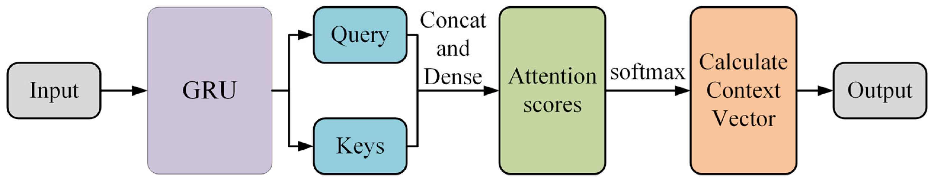
In this section, the proposed framework leverages GRU and Autoregressive Attention mechanisms to predict future displacements by modeling temporal dependencies within the GNSS time series. The combination of these methods enables accurate prediction of deformation by capturing both short-term variations and long-term trends. The following sections provide a detailed explanation of the methodology, as illustrated in the algorithm flowchart of Figure 1.
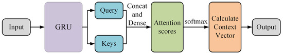
Figure 1.
Flowchart of the proposed GRU–Attention model.
The algorithm begins by inputting the three-dimensional GNSS displacement data. The data are first processed by a GRU module, which models the temporal dependencies and generates a sequence of hidden states. These hidden states serve as input to the attention mechanism, where two vectors, query and keys, are generated. The query and keys are concatenated and passed through a dense layer to compute the attention scores, which are subsequently normalized using the softmax function. The attention scores are then used to calculate a context vector that represents the weighted sum of the relevant past states. Finally, the context vector is used to predict future three-dimensional displacements.
2.1. GRU-Based Temporal Dependency Modeling
The GRU is a type of RNN specifically designed to handle sequential data. Unlike traditional RNN, the GRU employs gating mechanisms to control the flow of information across time steps, allowing it to retain relevant information and discard irrelevant details efficiently. This makes the GRU particularly well-suited for tasks involving time series, such as GNSS displacement prediction, where both short-term variations and long-term trends must be captured to achieve accurate predictions.
The GRU model processes GNSS deformation monitoring data through a sequential pipeline, as shown in Figure 2. First, the input data, including time-series displacement measurements, are fed into the GRU layer, which captures temporal dependencies by updating its hidden state through gated mechanisms. The update and reset gates control the flow of information of the input , allowing the model to retain long-term dependencies while filtering out irrelevant data. The GRU layer outputs a sequence representation, which is then passed through additional layers to enhance feature extraction. Finally, a dense output layer predicts the future displacement values and the model is trained using an optimization algorithm to minimize prediction error. All of the symbols are list in the Appendix A.
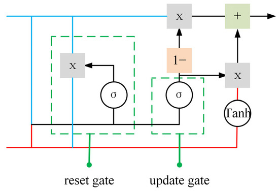
Figure 2.
Principle diagram of the GRU.
2.1.1. Reset Gate
The reset gate plays a critical role in determining how much of the information from the previous hidden state should be “forgotten” at each time step. This mechanism is essential for capturing important new patterns in the input sequence. When new information emerges, the reset gate selectively resets the previous memory, aiding the model in balancing long-term dependencies and short-term fluctuations. The reset gate operates by controlling the flow of information from the previous hidden state to the current time step [38]. Its output is bounded between 0 and 1 by a sigmoid activation function, effectively allowing the model to decide how much previous information to retain. The reset gate is computed as follows:
where is the reset gate at time step , represents the sigmoid activation function, is the weight matrix for the reset gate, is the hidden state from the previous time step, is the current input, and is the bias term for the reset gate. The reset gate is crucial in selectively forgetting irrelevant historical information. When sudden or new patterns arise in the data, the reset gate enables the model to discard outdated information, which is particularly useful when dealing with GNSS data that exhibits frequent short-term fluctuations.
2.1.2. Update Gate
The update gate determines how much information from the previous hidden state should be carried forward to the next time step and how much of the current candidate hidden state should be incorporated. This mechanism allows the model to retain relevant long-term dependencies while updating the hidden state to reflect the most recent information [39]. The update gate controls the weighted averaging between the previous hidden state and the current candidate hidden state. This balance allows the model to manage both long-term dependencies and short-term variations, preventing information from being gradually lost over time. The update gate is computed as follows:
where is the update gate at time step , is the weight matrix for the update gate, and is the bias term. The update gate’s key role is to balance the retention of past information with the incorporation of new information. This is particularly important when managing both long-term trends and short-term fluctuations, ensuring that the model can adaptively process time series data without losing valuable information from prior observations.
2.1.3. Candidate Hidden State
The candidate hidden state represents the potential contribution of the current time step to the hidden state. It is derived from the combination of the reset-controlled previous hidden state and the current input, offering a temporary estimate of the updated hidden state. The candidate hidden state is computed using both the reset-controlled previous hidden state and the current input [40]. The non-linear transformation of these two elements allows the model to produce a potential update for the current time step’s hidden state. The candidate hidden state is computed as follows:
where is the candidate hidden state at time step , is the hyperbolic tangent activation function, is the weight matrix for the candidate hidden state, is the reset gate output, and is the bias term. The candidate hidden state serves as the model’s prediction of the current time step’s contribution. It provides the foundation for updating the hidden state, allowing the model to dynamically adjust to new inputs, thereby enhancing prediction accuracy for GNSS displacements.
2.1.4. Hidden State
The hidden state update is the final step in the GRU, where the new hidden state is generated by combining the previous hidden state and the candidate hidden state. This process ensures that the model effectively balances long-term memory with the new information at each time step. The hidden state update is performed by the weighted combination of the previous hidden state and the candidate hidden state, where the weights are controlled by the update gate [41]. This mechanism allows the model to preserve long-term information while also updating its internal representation based on the current input. The hidden state update is computed as follows:
where is the updated hidden state at time step , and is the update gate output. The hidden state update ensures that both long-term and short-term information is preserved in the model. By adjusting the balance between previous and new information, the model is better equipped to handle complex temporal dependencies, leading to improved prediction accuracy for GNSS time series.
The GRU section provides a comprehensive breakdown of the key components that make up the gated recurrent unit, focusing on the reset gate, update gate, candidate hidden state, and hidden state update. Each part is detailed with an explanation of its function, significance, and mathematical formulation, highlighting the flow of information within the GRU [42]. This in-depth analysis demonstrates how the GRU architecture efficiently captures both long-term dependencies and short-term variations in time series data. To address the specific challenges of GNSS hydraulic engineering deformation monitoring, the GRU layer is configured to capture long-term dependencies and manage noisy, non-stationary deformation data. In our model, the GRU is set with 516 hidden units, which enables it to extract robust sequential features from the complex temporal patterns present in the GNSS measurements. This configuration is designed to effectively model gradual deformations over time, ensuring that the temporal dynamics critical for monitoring hydraulic structures are accurately represented.
2.2. Attention Mechanism for Weighted Context Aggregation
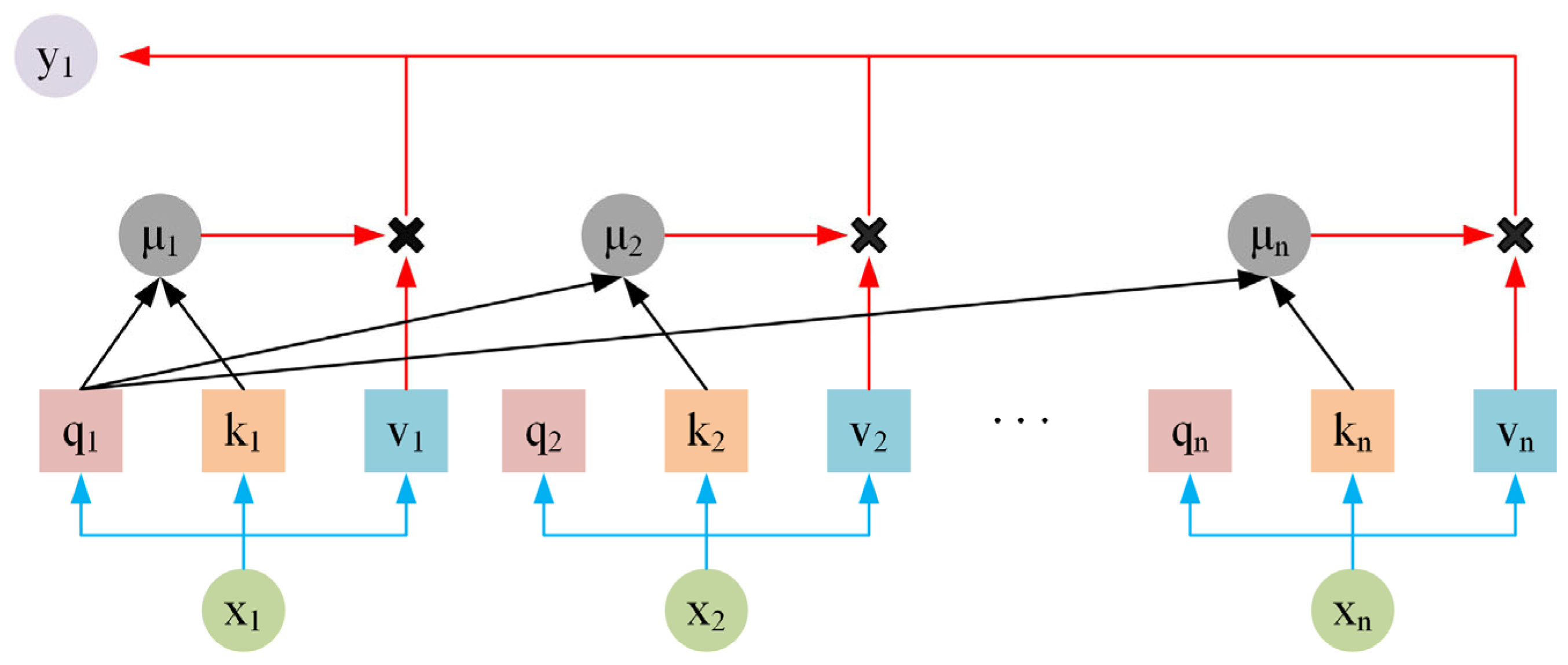
As shown in Figure 3, the Autoregressive Attention section systematically details the key components, including query and key generation, attention score computation, context vector calculation, and the final prediction. Through these processes, the model selectively focuses on important past observations and synthesizes this information into a precise prediction of future values. All of the symbols are list in the Appendix A.
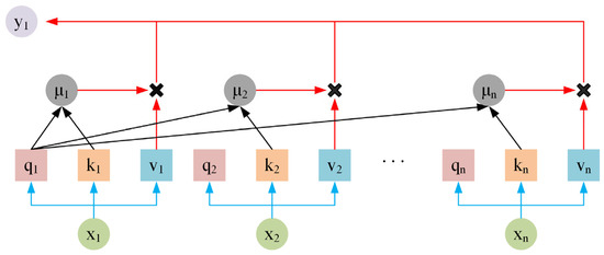
Figure 3.
Principle diagram of Autoregressive Attention mechanism.
2.2.1. Query and Key Generation
In the Autoregressive Attention mechanism, the generation of queries and keys is critical for establishing the relevance between the current input and past observations. This process allows the model to focus on important historical information while making predictions. By generating queries and keys, the model dynamically determines which previous data points are most relevant for the current prediction [43]. Queries represent the current input, while keys represent past information. The attention mechanism computes the relevance score between the query and each key, helping the model decide which past information should be attended to in the prediction process. The queries and keys are generated as follows:
where is the query at time step , is the key at the previous time step, is the value at the previous time step, and are the weight matrices for the query and key generation, and and are the hidden states at the current and previous time steps, respectively. Query and key generation enable the model to determine the relevance of historical data in the prediction process. By forming these vectors, the Autoregressive Attention mechanism selectively attends to significant patterns from past observations, which is essential for accurately forecasting GNSS displacement trends.
2.2.2. Attention Score Computation
Attention scores represent the importance of each past time step in predicting the current output. The scores indicate which previous observations should contribute more or less to the model’s understanding of the data. Computing attention scores allows the model to weigh historical data effectively and focus on the most relevant information [44]. The attention scores are computed by taking the dot product of the query and key vectors, followed by applying a function to normalize the scores. This process ensures that the attention weights are positive and sum to 1, emphasizing the most relevant past information. Attention scores are computed as follows:
where is the attention score at time step , and normalizes the dot product between the query and key . Computing attention scores is central to the Autoregressive Attention mechanism, as it enables the model to allocate different weights to past observations. This allows for an adaptive focus on the most relevant time steps, improving the model’s capacity to make accurate predictions, particularly when dealing with GNSS displacement.
2.2.3. Context Vector Calculation
The context vector is the weighted sum of the hidden states from previous time steps, representing a summary of the most relevant historical information for the current prediction. It allows the model to synthesize past data into a single vector that guides the final prediction [45]. The context vector is computed by multiplying the attention scores with the corresponding hidden states of past time steps. This process aggregates the information from relevant past inputs, effectively compressing them into a single vector that encapsulates the most important information for the current time step. The context vector is calculated as follows:
where is the context vector at time step , is the attention score at time step , and is the hidden state at time step . The context vector encapsulates the most relevant historical information, enabling the model to incorporate long-term dependencies into the current prediction. This synthesis of past data ensures that the model can effectively handle complex temporal patterns, enhancing the prediction of GNSS displacements.
2.2.4. Final Prediction
The final prediction is generated by combining the context vector with the current hidden state, allowing the model to make a well-informed decision based on both past and present data. This step is crucial for outputting accurate predictions in GNSS time series tasks. The final prediction is made by passing the context vector and the current hidden state through a dense layer. This combination allows the model to incorporate both short-term and long-term dependencies, producing a precise forecast of the target variable. The final prediction is computed as follows:
where is the predicted output at time step , is the context vector, and is the current hidden state. The dense layer linearly combines these inputs to produce the final prediction. The final prediction step allows the Autoregressive Attention mechanism to leverage both long-term dependencies and short-term dynamics. This integration of information ensures that the model provides highly accurate predictions, essential for forecasting GNSS displacements in engineering applications.
The attention mechanism is tailored to enhance the model’s focus on the most relevant temporal segments in GNSS deformation data. In our Autoregressive Attention layer, the last time step of the input sequence is used as the query, while all preceding time steps serve as keys. This design emphasizes recent observations while still integrating valuable historical context. The attention scores are calculated by concatenating the repeated query with the keys, processing them through a dense layer with tanh activation, and applying a learned weight vector and bias. This approach effectively mitigates noise and extracts critical features, thereby improving the accuracy of deformation predictions.
3. Experiment and Results
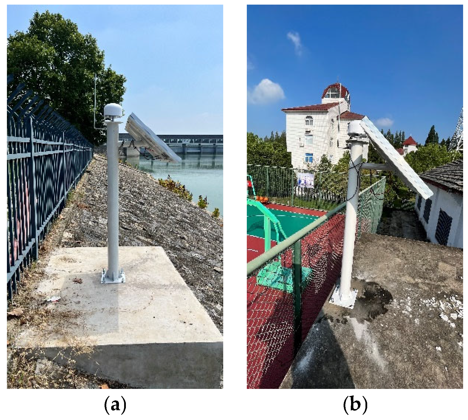
The experiment was conducted at the Sanhe Sluice of Hongze Lake, Jiangsu, China, a critical location for hydrological monitoring, as shown in Figure 4. The experimental period spanned from 10 September 2023, to 10 September 2024, covering a full year to capture seasonal variations. During this time, multi-constellation GNSS signals were utilized, including BeiDou (B1I, B2I), Galileo (E1B/C, E5b), and GPS (L1C/A, L2C), with a sampling frequency of 1 Hz to ensure high temporal resolution and precise data collection. This setup enabled comprehensive analysis and evaluation of the GNSS’ performance in real-world conditions.

Figure 4.
The monitoring site used for the experiment ((a) is the monitoring site, (b) is the reference site)).
The GNSS data processing strategy is as follows: Ambiguity resolution is conducted using the MLAMBDA method, while multipath error is addressed using a stellar day filter within the observational domain. The Saastamoinen Model coupled with a Random Walk method is employed for troposphere error correction, while the ionosphere error is mitigated using a broadcast model. Outputs are recorded at 1 h intervals, and data are smoothed using the Rauch–Tung–Striebel Smoother Filter Method.
3.1. Data Analysis
In this section, a comprehensive analysis of the GNSS displacements used in the study is presented. The focus is on both the raw displacement values and their dynamic derivatives to better understand the movement patterns and trends in the time series. Furthermore, the impact of data preprocessing, specifically normalization, on model performance is examined. Visual representations are provided to illustrate the raw and processed data, along with the effect of normalization on the training process, which plays a crucial role in improving model convergence and accuracy.
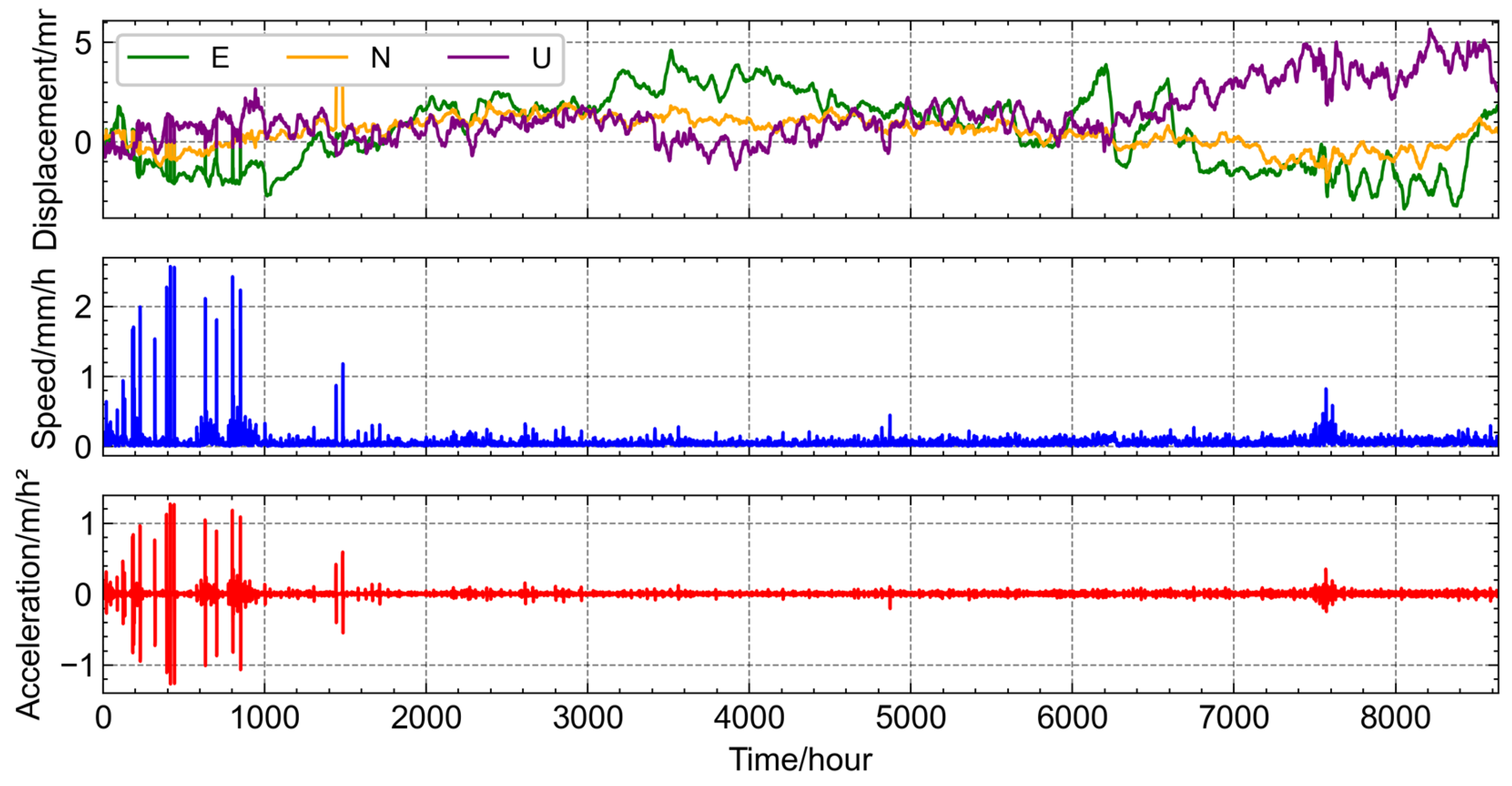
As shown in Figure 5, the first subfigure presents the GNSS displacement over time. Due to the use of an imperfect positioning strategy at the initial stage, the first 1000 h of data exhibit a high number of abrupt outliers, with displacement variations reaching up to 5 mm. After refining the positioning strategy, the accuracy of the results improved significantly. In the velocity subfigure, a similar pattern is observed, where frequent outliers appear within the first 1000 h, with variations reaching up to 2 mm/h. Additionally, there are minor fluctuations around the 1500th hour and 7500th hour marks, but the velocity remains relatively stable during the rest of the time. The acceleration subfigure follows the same trend, with the most abrupt outliers in the first 1000 h, where variations reach 1 mm/hour2. Small fluctuations also occur near the 1500th hour and 7500th hour marks, but the overall acceleration is stable beyond these periods. This figure effectively highlights the initial phase of noise and the overall data stability after the correction of the positioning strategy.

Figure 5.
Time series diagram of GNSS and extended differential data.
In this experiment, the GRU–Attention model is designed to effectively capture temporal dependencies and enhance predictive accuracy. The model consists of a GRU layer with 516 hidden units, which enables it to extract sequential features while maintaining temporal correlations. The Autoregressive Attention mechanism follows, comprising 256 units to refine the learned representations by focusing on important temporal patterns. The final output layer is a dense layer with five linear activation units, corresponding to the five-dimensional output required for prediction. The model is trained using the Adam optimizer and mean squared error as the loss function, ensuring efficient convergence and robust performance across different displacement directions.
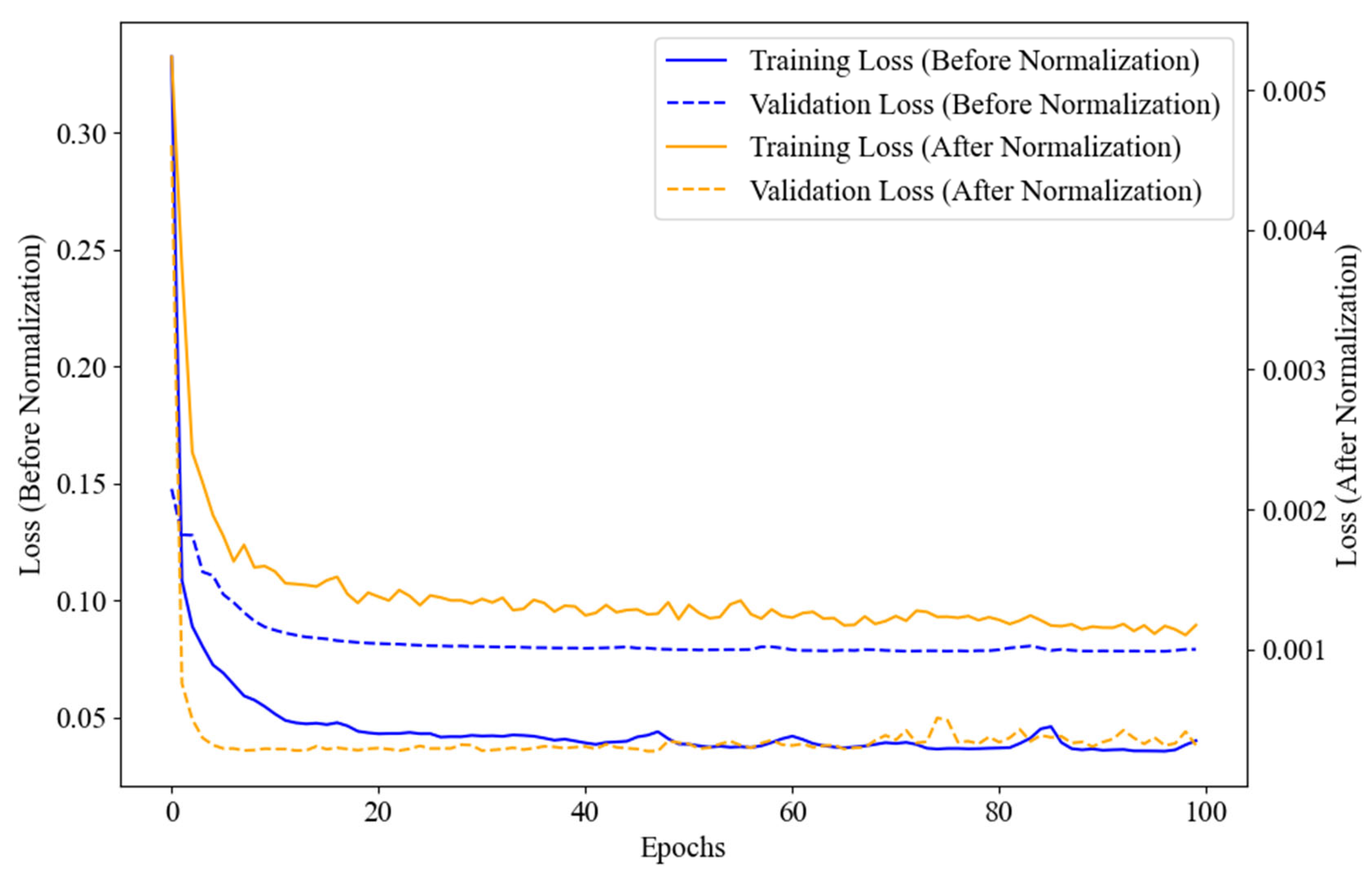
Figure 6 presents the loss diagram of the normalization and originals, which contains four curves. For the original data, the training loss curve initially rises to 0.25 and then stabilizes around the 10th epoch. However, frequent fluctuations occur between the 10th and 50th epochs. The test loss curve for the original data shows a similar trend, rising to 0.025 initially, then stabilizing around the 10th epoch, but it also exhibits frequent fluctuations between the 10th and 50th epochs. In contrast, after normalization, the training loss curve converges smoothly from 0.005 to 0.0008 within the first 7 epochs and remains stable without the fluctuations observed before normalization. Similarly, the test loss curve for the normalized data converges from 0.004 to 0.0003 within the first 7 epochs, maintaining stability afterward. This figure clearly illustrates the significant improvement in convergence and stability achieved through GNSS data normalization.
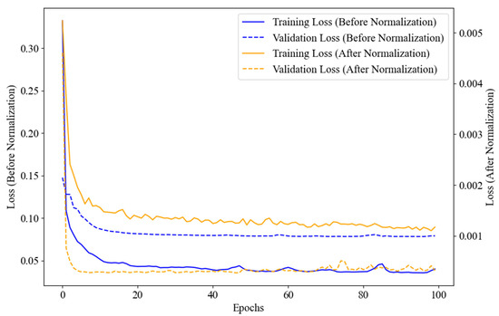
Figure 6.
The loss diagram of the normalization and originals.
3.2. Model Construction
In this section, the architecture and performance of the proposed GRU–Attention model are explored. The model leverages the strengths of the GRU in capturing temporal dependencies and the Autoregressive Attention mechanism to focus on the most relevant time steps for accurate displacement prediction. A detailed analysis is provided through three key visualizations: an attention heatmap to illustrate the attention weights applied during prediction, a time series plot showing the model’s predictive performance on the test dataset, and a residual distribution plot to assess the accuracy and potential biases of the model’s predictions. Together, these elements offer a comprehensive overview of the model’s construction and performance.
Figure 7 presents the absolute error of the GRU–Attention model across the three directional components in the training dataset. Overall, the model exhibits relatively poor fitting performance, with a maximum fluctuation range of approximately 0.8 mm. Within the 0 to 3000 h interval, the absolute error shows an increasing trend, gradually rising to around 0.6 mm. From 3000 to 5500 h, the error generally decreases, except for a brief period between 3500 and 4000 h, where sudden spikes reaching 0.75 mm are observed. In the 5500 to 7000 h interval, the error begins to rise again, peaking at 0.8 mm before gradually decreasing to approximately 0.2 mm toward the end of the observation period. These variations suggest that while the model captures general displacement trends, its accuracy fluctuates over time, particularly in certain intervals, highlighting the need for further refinement to improve predictive stability.
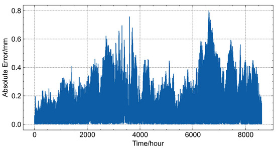
Figure 7.
Absolute error of the GRU–Attention model across three directions in the training dataset.
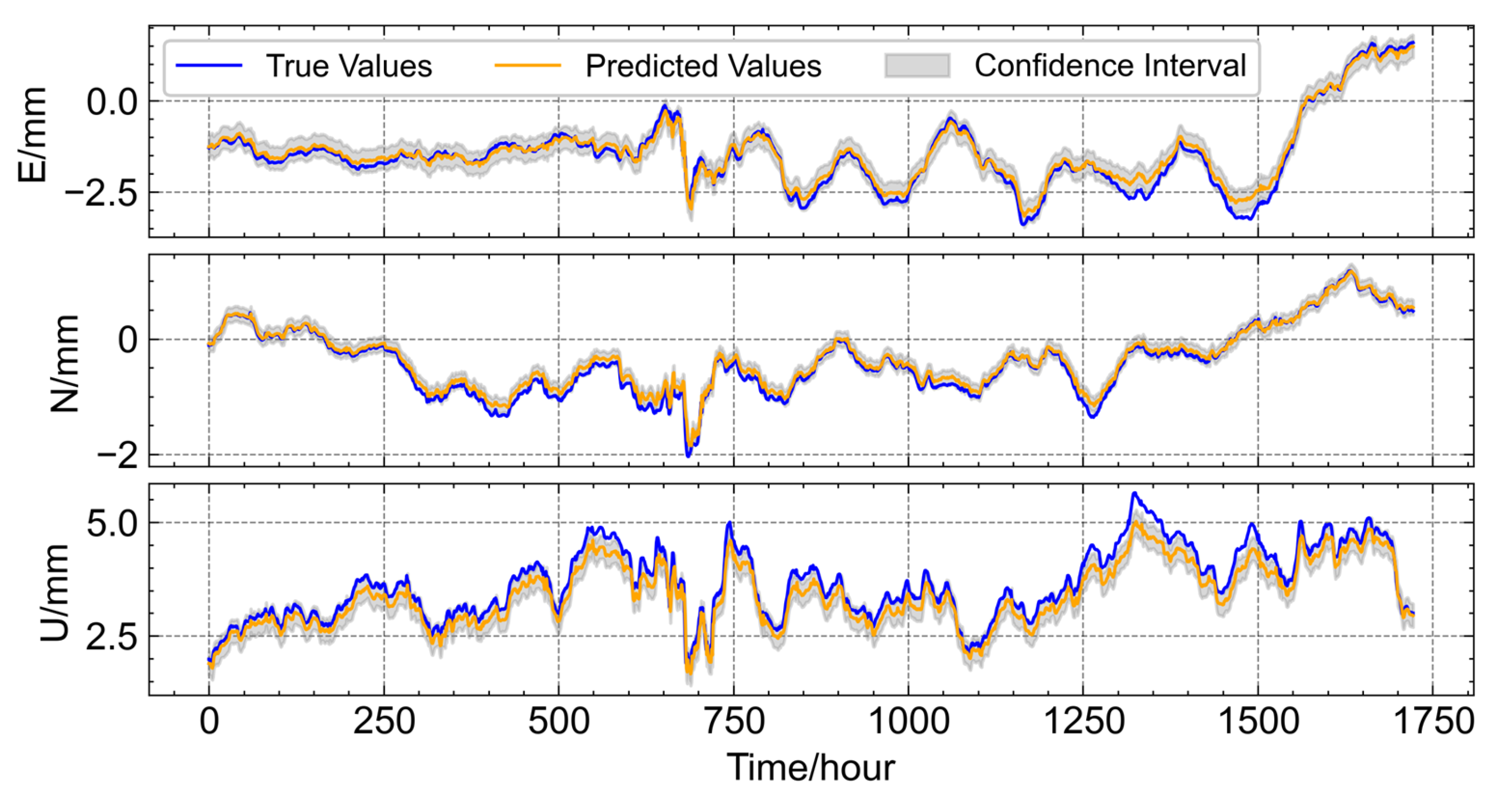
Figure 8 shows the performance of the GRU–Attention model on the test dataset. GRU is configured with 1024 hidden units, while the Autoregressive Attention mechanism uses 32 units. The model demonstrates strong overall performance across the various directional components. In the east (E) direction, the predicted results align well with the actual observations, with only minor discrepancies observed around the 650th and 1500th hours. The performance in the north (N) direction is comparable to the E direction but shows a slight improvement, with a small deviation occurring near the 700th hour. In contrast, the performance in the up (U) direction is relatively weaker, although the predicted time series closely follows the trend of the original observations. Discrepancies of approximately 0.5 mm are noted in several intervals, such as between the 500th and 600th and 1200th and 1400th hours. These differences highlight the challenges of accurately predicting vertical displacements and suggest potential areas for further model refinement, such as integrating additional sensor data or enhancing feature extraction techniques to improve performance in the three directions. In summary, the proposed GRU–Attention model exhibits high prediction accuracy across all directions, with the N direction showing the best performance and the U direction exhibiting minor differences from the actual measurements.
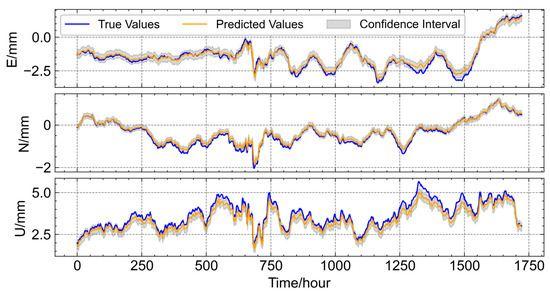
Figure 8.
Performance of the GRU–Attention Model in Multi-Directional Displacement Prediction.
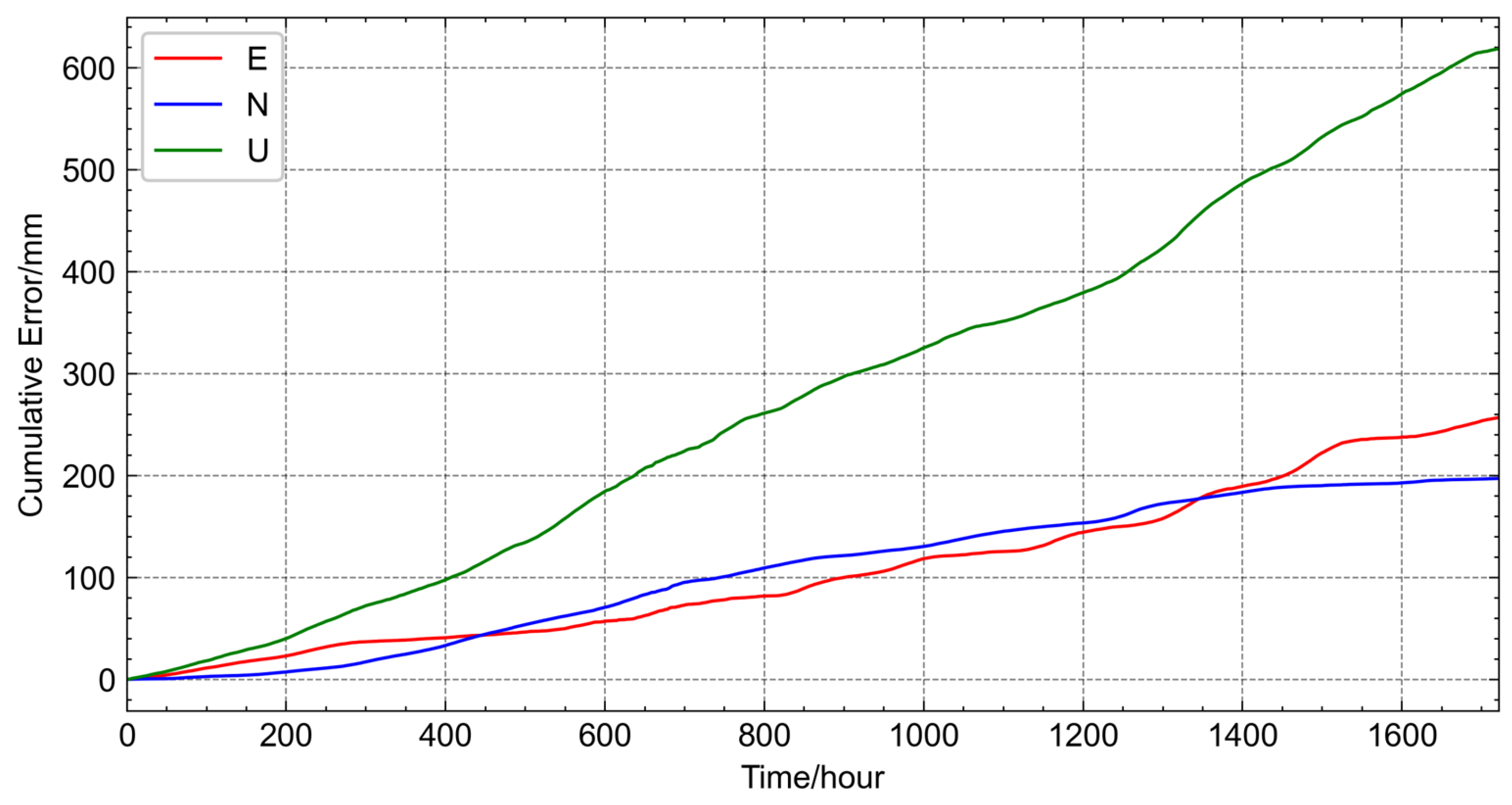
Figure 9 illustrates the cumulative error in the test dataset for each directional component. Both the E and N directions demonstrate relatively low cumulative errors. The linear fit slope for the E direction is approximately 0.15, indicating a gradual increase in cumulative error over time. Similarly, the N direction shows a linear fit slope of about 0.11, with the cumulative error curve exhibiting a slightly higher magnitude than the E direction between the first 1400 h but falling below the E direction after the 1400 h interval. In contrast, the U direction displays a significantly larger cumulative error, with a linear fit slope of around 0.36. The cumulative error curve for the U direction is notably higher than that of both the E and N directions throughout the entire test period.
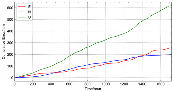
Figure 9.
Cumulative Error Analysis of the GRU–Attention Model in Multi-Directional Displacement Prediction.
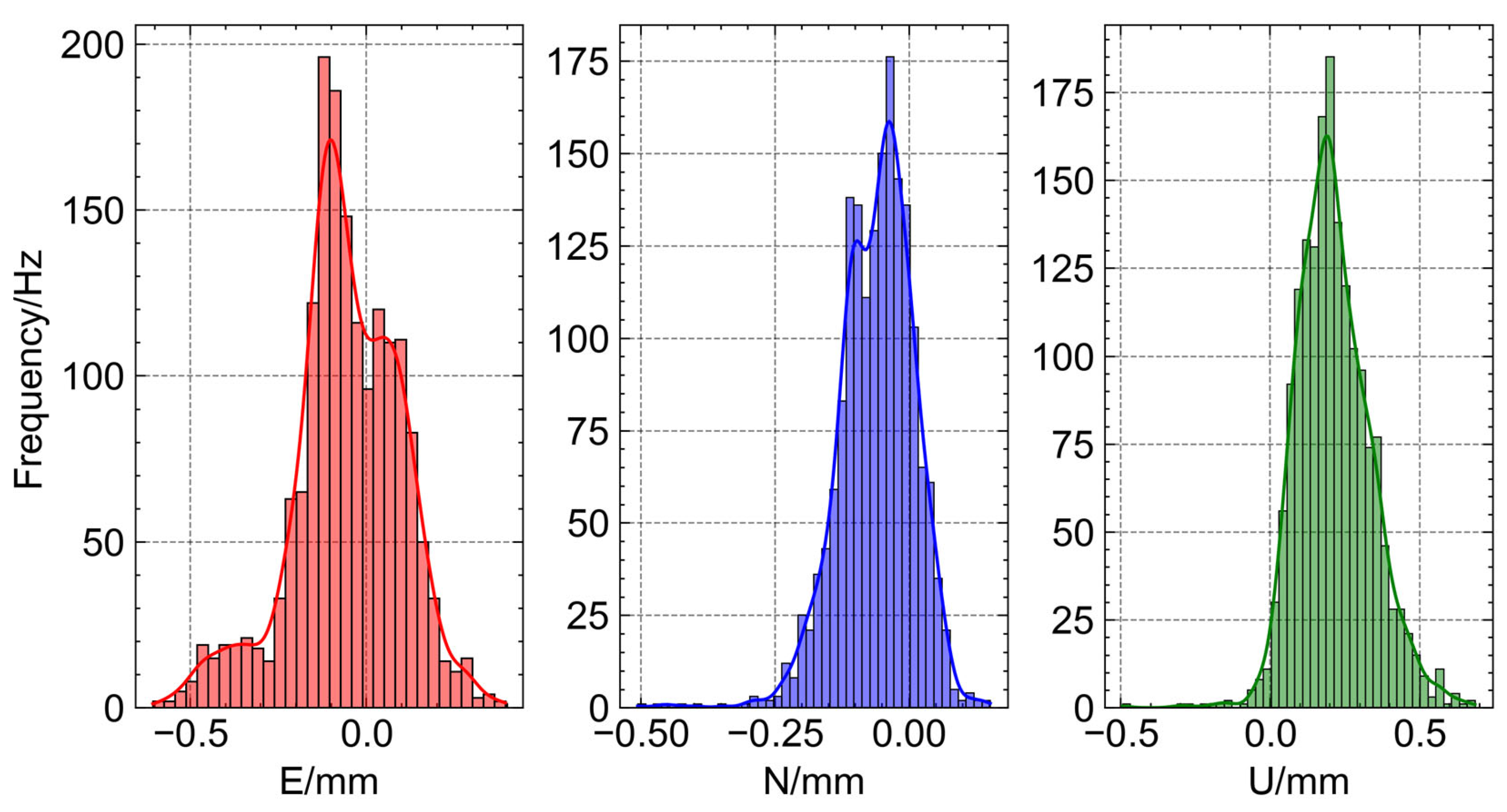
Figure 10 presents the error distribution histograms for the test set across the E, N, and U directions, revealing distinct characteristics in each direction. In the E direction, errors generally follow a normal distribution with a central value of approximately −0.1 mm and a range from −0.6 mm to 0.3 mm. Most data points are concentrated between −0.3 mm and 0.3 mm, with only a small portion falling between −0.6 mm and −0.3 mm. The N direction shows an even closer alignment to a normal distribution, with a central value around −0.1 mm and a range from −0.6 mm to 0.2 mm. Errors are predominantly within −0.2 mm to 0.2 mm, with few outliers between −0.6 mm and −0.2 mm. In contrast, the U direction exhibits a broader error distribution, with a central value of about 0.2 mm and a range from −0.1 mm to 0.9 mm. Most errors are concentrated between −0.1 mm and 0.6 mm, while some extend into the 0.6 mm to 0.9 mm range. Overall, while the E and N directions demonstrate relatively narrow error ranges and better adherence to normal distributions, the U direction shows larger deviations and a wider spread, highlighting greater challenges in vertical measurements.
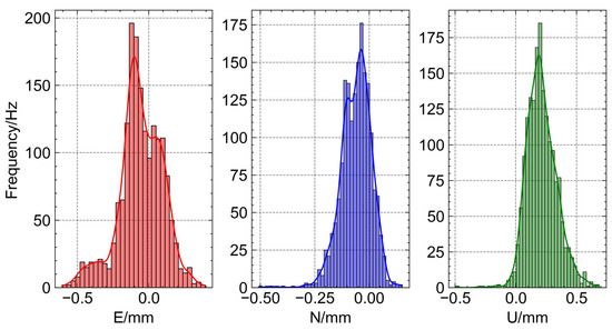
Figure 10.
Error distribution histograms of the GRU–Attention model in Multi-Directional Displacement Prediction.
3.3. Comparison with Alternative Method
In this section, the proposed GRU–Attention model is compared with existing models used for deformation prediction in hydraulic engineering. The selected baseline models include CNN-GRU and VMD-LSTM, both of which have demonstrated effectiveness in this field. The CNN-GRU model leverages convolutional layers to extract spatial features while utilizing GRU for temporal dependencies, enhancing its ability to capture complex deformation patterns [32]. Meanwhile, the VMD-LSTM model employs Variational Mode Decomposition (VMD) to decompose non-linear deformation signals into intrinsic mode functions, allowing LSTM to model long-term dependencies more effectively [28]. These models serve as strong benchmarks for evaluating the performance of the GRU–Attention model.
Figure 11 illustrates the absolute error distribution of the three models in the test dataset for three-dimensional displacement prediction. The GRU–Attention model, represented in red, exhibits the best overall performance, maintaining the smallest fluctuation range. Its maximum error reaches approximately 0.7 mm within the 1250 to 1500 h interval, demonstrating stable and consistent predictions. The VMD-LSTM model, shown in blue, performs moderately well but exhibits frequent fluctuations throughout the test interval, with its largest deviation reaching around 2 mm near the 1600 h mark. The CNN-GRU model, represented in green, performs the worst, with fewer fluctuations compared to VMD-LSTM but exhibiting a maximum deviation of approximately 2.9 mm around the 700 h interval. Overall, the results indicate that the GRU–Attention model provides the most stable and accurate predictions, effectively minimizing errors and maintaining consistency. The VMD-LSTM model demonstrates moderate accuracy but suffers from frequent fluctuations, while the CNN-GRU model exhibits the largest deviations, highlighting its limitations in multi-step displacement forecasting. These findings further confirm the superior predictive capability of the GRU–Attention model in deformation monitoring applications.
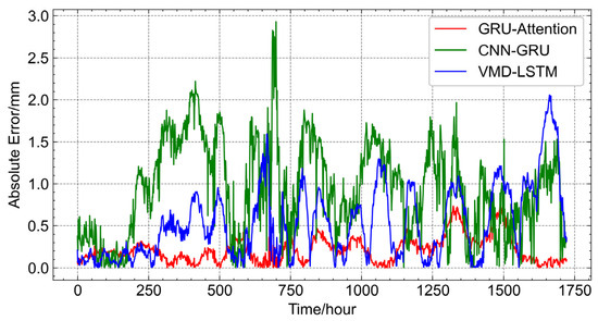
Figure 11.
Absolute error distribution of three models in the test dataset.
Figure 12 illustrates the multi-step prediction results of the three models over a 24 h forecasting horizon. The red line represents the GRU–Attention model, the green line corresponds to the CNN-GRU model, and the blue line denotes the VMD-LSTM model. In the E direction, the GRU–Attention model achieves the best performance, with prediction errors fluctuating around 1.5 mm. The smallest deviation occurs at the 5th hour, where the predicted displacement is nearly identical to the actual value, while the largest deviation of approximately 2 mm appears at the initial stage. The CNN-GRU model ranks second, with errors fluctuating around 2.5 mm, reaching a maximum deviation of 3.5 mm at the 14th hour and a minimum of 2 mm at the 6th hour. The VMD-LSTM model performs the worst, with deviations around 5 mm, showing the smallest error of 3 mm at the 24th hour and the largest deviation of approximately 6.5 mm at the 1st hour. A similar trend is observed in the N direction. The GRU–Attention model again achieves the best results, with errors fluctuating around 0 mm, except for the 5–15 h interval, where the maximum deviation of about 1 mm appears at the beginning. The CNN-GRU model follows, with deviations around 1 mm, reaching a maximum of 2 mm at the initial stage and a minimum of 0 mm at the 10th hour. The VMD-LSTM model exhibits the largest errors, fluctuating around 5 mm, with the smallest deviation of 3 mm at the 8th hour and the largest deviation of approximately 7 mm at the 4th hour.
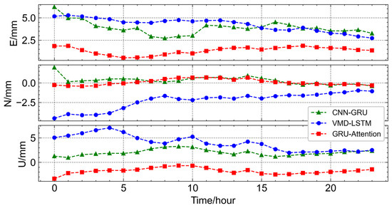
Figure 12.
Error comparison diagram of the multi-step predictions.
In the U direction, the GRU–Attention model continues to show superior performance, with errors fluctuating around −1 mm, reaching the smallest deviation of nearly 0 mm at the 8th–10th hour interval and the largest deviation of approximately −3 mm at the initial stage. The CNN-GRU model ranks second, with errors fluctuating around 2 mm, peaking at 3.5 mm at the 10th hour and reaching a minimum of 1 mm at the 16th hour. The VMD-LSTM model performs the worst, with deviations around 5 mm, showing the smallest error of 3 mm at the 4th hour and the largest deviation of approximately 7 mm at the 17th hour. Overall, Figure 12 demonstrates that the GRU–Attention model consistently outperforms the other two models across all three directions, maintaining the lowest prediction errors and the closest alignment with actual displacement values. The CNN-GRU model follows as the second-best performer, while the VMD-LSTM model exhibits the largest deviations, indicating lower predictive accuracy.
Table 1 presents the comparative statistics of multi-step prediction performance for the three models. mean squared error (MSE) measures the average squared difference between predicted and actual values, penalizing larger errors more heavily to emphasize significant deviations. Mean Absolute Error (MAE) calculates the average absolute difference between predicted and actual values, providing a straightforward measure of overall prediction accuracy. Coefficient of Determination (R2) evaluates the proportion of variance in the actual values that is explained by the model, indicating how well the predictions fit the observed data. In terms of MSE, the GRU–Attention model achieves 1.98 mm, representing a 27.7% reduction compared to CNN-GRU at 2.74 mm and a 36.5% reduction compared to VMD-LSTM at 3.12 mm. The MAE for GRU–Attention is 7.59 mm, which is 59.1% lower than CNN-GRU at 18.55 mm and 72.4% lower than VMD-LSTM at 27.48 mm, indicating significantly improved predictive precision. Additionally, the GRU–Attention model achieves the highest R2 at 0.733, outperforming CNN-GRU at 0.514 by 42.6% and VMD-LSTM at 0.457 by 60.4%, highlighting its stronger correlation with actual displacement values. These results clearly demonstrate that the GRU–Attention model outperforms the other two models in all evaluation metrics, offering more accurate and reliable multi-step displacement forecasting.

Table 1.
Comparison statistics of multi-step prediction.
4. Discussion
This study investigates the performance of a GRU–Attention model for multi-step displacement prediction and compares it with CNN-GRU and VMD-LSTM approaches. Our experimental results indicate that the GRU–Attention model outperforms the alternative models across several key metrics. For instance, in the test dataset, the GRU–Attention model consistently exhibited lower MSE, MAE, and higher R2 compared to both CNN-GRU and VMD-LSTM. These improvements suggest that the integration of an autoregressive attention mechanism with GRU layers enables more effective modeling of temporal dependencies and nuanced displacement patterns.
A horizontal comparison across the three spatial directions further underscores the model’s strengths and limitations. In the E and N directions, the GRU–Attention model demonstrates strong alignment with actual observations, with only minor discrepancies noted in specific time intervals. Notably, the N direction shows the best performance overall, which may be attributed to more stable displacement characteristics or reduced measurement noise in that axis. However, the U direction presents a challenge, with a broader error distribution and larger deviations. This phenomenon is consistent with prior research that identifies vertical displacement prediction as inherently more complex, likely due to the higher sensitivity of vertical measurements to sensor noise, environmental perturbations, and intricate soil–structure interactions.
From a longitudinal perspective, the model’s performance varies over time. Analysis of the training dataset reveals that while the model captures general trends, the absolute error demonstrates a non-monotonic evolution. In the early training phase, error increases gradually, reaches a plateau, and then exhibits fluctuations before declining towards the end of the training period. These temporal dynamics may reflect the model’s sensitivity to long-term dependencies and intermittent disturbances in the training data, emphasizing the need for further model optimization.
Comparisons with existing studies highlight both advancements and areas for improvement. While previous approaches using CNN-GRU and VMD-LSTM have achieved reasonable prediction accuracies, our results suggest that the GRU–Attention model offers enhanced predictive capability, particularly in handling spatial–temporal complexities. However, discrepancies in the vertical direction and certain temporal intervals suggest that the current model architecture may not fully capture all underlying dynamics. This limitation underscores the importance of integrating additional sensor modalities and refining feature extraction techniques.
In conclusion, our findings validate the efficacy of the GRU–Attention framework in multi-step displacement forecasting, demonstrating its superior performance relative to established methods. Nonetheless, the observed performance variability, particularly in vertical displacement prediction, points to the need for further research. Future work should focus on incorporating richer datasets, exploring hybrid model architectures, and developing advanced attention mechanisms to mitigate the impact of noise and capture more complex deformation behaviors. Such enhancements will be critical to advancing predictive accuracy and reliability in the context of hydraulic engineering deformation monitoring.
5. Conclusions
This study presents a comprehensive investigation into multi-step displacement prediction by developing and evaluating a GRU–Attention model. The research process involved designing a model architecture that integrates a GRU layer with an autoregressive attention mechanism and comparing its performance with alternative approaches including CNN-GRU and VMD-LSTM. Extensive experiments were performed on both training and test datasets across three directional components to assess the model’s ability to capture temporal dependencies and predict displacements accurately. Detailed error analyses, including absolute error trends, cumulative error evaluations, and error distribution histograms, revealed the model’s behavior over different time intervals and directions.
The results indicate that the GRU–Attention model achieves superior performance in multi-step displacement prediction compared to alternative methods. The model demonstrates lower prediction errors and higher stability in the east and north directions, while it shows challenges in accurately predicting vertical displacements. The integration of the attention mechanism with GRU layers enhances the model’s capacity to capture subtle temporal patterns and improve forecasting accuracy. These findings provide an abstract overview of the predictive process and reinforce the idea that advanced temporal modeling techniques contribute to improved deformation monitoring in hydraulic engineering.
The implications of this research are two-fold. First, the demonstrated efficacy of the GRU–Attention model offers valuable insights into the field of structural health monitoring and highlights the potential of combining recurrent neural networks with attention mechanisms to enhance prediction performance. Second, the study provides a methodological framework that encourages future research to incorporate additional sensor data and hybrid architectures to address complex temporal and spatial dependencies. Overall, the contributions of this study pave the way for more reliable and accurate deformation monitoring systems, which are critical for the safety and longevity of hydraulic structures.
Moving forward, there are several avenues for refinement and improvement. One key direction is to enhance the model’s prediction accuracy for U displacements, which will further bolster its utility in comprehensive deformation monitoring. Additionally, optimizing the model for real-time applications could increase its feasibility for use in large-scale infrastructure projects, where immediate and continuous data processing is essential. These improvements would expand the applicability of the GRU–Attention model, allowing it to be deployed across a broader range of infrastructure types and environmental conditions, contributing to more effective health monitoring systems and proactive maintenance strategies. By integrating such enhancements, the model has the potential to play a central role in the future of infrastructure management, improving safety, reducing maintenance costs, and prolonging the operational lifespan of critical structures.
Author Contributions
Conceptualization, H.L. and Y.Z.; methodology, H.L. and Y.X.; software, Y.X. and A.D.; validation, H.L., Y.X. and J.X.; formal analysis, J.X. and X.L.; investigation, X.L. and J.D.; resources, A.D. and J.X.; data curation, Y.X. and X.L.; writing—original draft preparation, H.L. and J.D.; writing—review and editing, Y.Z. and A.D.; visualization, X.L. and Y.X.; supervision, Y.Z.; project administration, H.L. and Y.Z.; funding acquisition, Y.Z. All authors have read and agreed to the published version of the manuscript.
Funding
This research was funded by Key Laboratory of New Technology for Construction of Cities in Mountain Area, Ministry of Education, grant number LNTCCMA-20230112; Major Scientific and Technological Projects of the Ministry of Water Resources, grant number SKS-2022162; Jiangsu Provincial Department of Water Resources, grant numbers 2022050, 2022083 and 2023031, and the Jiangsu Hydraulic Research Institute, grant number 2023z036.
Data Availability Statement
The original contributions presented in this study are included in the article. Further inquiries can be directed to the corresponding author.
Conflicts of Interest
The authors declare no conflicts of interest.
Appendix A
| Symbol | Brief Description |
|---|---|
| X | Input GNSS time series |
| σ | sigmoid activation function |
| hyperbolic tangent activation function | |
| Input of the Attention and output of the GRU | |
| key at the previous time step | |
| value at the previous time step | |
| attention score at time step t |
References
- Tretyak, K.; Bisovetskyi, Y.; Savchyn, I.; Korlyatovych, T.; Chernobyl, O.; Kukhtarov, S. Monitoring of spatial displacements and deformation of hydraulic structures of hydroelectric power plants of the Dnipro and Dnister cascades (Ukraine). J. Appl. Geod. 2024, 18, 345–357. [Google Scholar] [CrossRef]
- Yue, B.; Zhang, Z.; Zhang, W.; Luo, X.; Zhang, G.; Huang, H.; Wu, X.; Bao, K.; Peng, M. Design of an Automatic Navigation and Operation System for a Crawler-Based Orchard Sprayer Using GNSS Positioning. Agronomy 2024, 14, 271. [Google Scholar] [CrossRef]
- Wos, P.; Dindorf, R.; Takosoglu, J. The electro-hydraulic lifting and leveling system for the bricklaying robot. In Proceedings of the International Scientific-Technical Conference on Hydraulic and Pneumatic Drives and Control, Trzebieszowice, Poland, 21–23 October 2020; Springer International Publishing: Cham, Switzerland, 2020; pp. 216–227. [Google Scholar]
- Yamamoto, Y.; Kikuuwe, R. End-Effector Position Estimation and Control of Hydraulic Excavators with Total Stations. In Proceedings of the 2024 IEEE/SICE International Symposium on System Integration (SII), Ha Long, Vietnam, 8–11 January 2024; pp. 345–350. [Google Scholar]
- Wang, Y.; Ren, P.; Xiong, W.; Peng, X. Strain analysis and non-destructive monitoring of the two-stage hydraulic-driven piston compressor for hydrogen storage. J. Energy Storage 2024, 94, 112494. [Google Scholar] [CrossRef]
- Beckett, H.A.; Bryant, C.; Neeman, T.; Mencuccini, M.; Ball, M.C. Plasticity in branch water relations and stem hydraulic vulnerability enhances hydraulic safety in mangroves growing along a salinity gradient. Plant Cell Environ. 2024, 47, 854–870. [Google Scholar] [CrossRef]
- Dorji, Y.; Isasa, E.; Pierick, K.; Cabral, J.S.; Tobgay, T.; Annighöfer, P.; Schuldt, B.; Seidel, D. Insights into the relationship between hydraulic safety, hydraulic efficiency and tree structural complexity from terrestrial laser scanning and fractal analysis. Trees 2024, 38, 221–239. [Google Scholar] [CrossRef]
- Purnell, D.; Dabboor, M.; Matte, P.; Peters, D.; Anctil, F.; Ghobrial, T.; Pierre, A. Observations of River Ice Breakup Using GNSS-IR, SAR and Machine Learning. IEEE Trans. Geosci. Remote Sens. 2024, 62, 5800613. [Google Scholar] [CrossRef]
- Li, H.; Nie, G.; Chen, D.; Wu, S.; Wang, K. Constrained MLAMBDA method for multi-GNSS structural health monitoring. Sensors 2019, 19, 4462. [Google Scholar] [CrossRef]
- Li, H.; Nie, G.; Wang, J.; Wu, S.; He, Y. A novel partial ambiguity method for multi-GNSS real-time kinematic positioning. J. Navig. 2022, 75, 540–553. [Google Scholar] [CrossRef]
- Li, H.; Nie, G.; Wu, S.; He, Y. Sequential ambiguity resolution method for poorly-observed GNSS data. Remote Sens. 2021, 13, 2106. [Google Scholar] [CrossRef]
- Lee, C.M.; Fu, C.Y.; Lan, W.H.; Kuo, C.Y. Performance evaluation of different reflected signal extraction methods on GNSS-R derived sea level heights. Adv. Space Res. 2024, 74, 89–104. [Google Scholar] [CrossRef]
- Li, C.; Yang, P.; Zhang, T.; Guo, J. Periodic signal extraction of GNSS height time series based on adaptive singular spectrum analysis. Geod. Geodyn. 2024, 15, 50–60. [Google Scholar] [CrossRef]
- Li, J.; Yang, D.; Wang, F.; Yang, L. A solution to the problem of height overcompensation in GNSS-IR corn height measurements: A canopy reflectance calibration model. Remote Sens. Lett. 2024, 15, 66–76. [Google Scholar] [CrossRef]
- Li, W.; Guo, J. Extraction of periodic signals in Global Navigation Satellite System (GNSS) vertical coordinate time series using the adaptive ensemble empirical modal decomposition method. Nonlinear Process. Geophys. 2024, 31, 99–113. [Google Scholar] [CrossRef]
- Kano, M.; Tanaka, Y.; Sato, D.; Iinuma, T.; Hori, T. Data assimilation for fault slip monitoring and short-term prediction of spatio-temporal evolution of slow slip events: Application to the 2010 long-term slow slip event in the Bungo Channel, Japan. Earth Planets Space 2024, 76, 57. [Google Scholar] [CrossRef]
- Jiang, W.; Wang, J.; Li, Z.; Li, W.; Yuan, P. A new deep self-attention neural network for GNSS coordinate time series prediction. GPS Solut. 2024, 28, 3. [Google Scholar] [CrossRef]
- Vu, T.H.; Vu, N.Q.; Van Thieu, N. Spatial prediction of bridge displacement using deep learning models: A case study at Co Luy bridge. In Applications of Artificial Intelligence in Mining, Geotechnical and Geoengineering; Elsevier: Amsterdam, The Netherlands, 2024; pp. 437–461. [Google Scholar]
- Qiu, D.; Wang, T.; Ye, Q.; Huang, H.; Wang, L.; Duan, M.; Luo, D. A deformation prediction approach for supertall building using sensor monitoring system. J. Sens. 2019, 2019, 9283584. [Google Scholar] [CrossRef]
- Lian, X.; Li, Z.; Yuan, H.; Hu, H.; Cai, Y.; Liu, X. Determination of the stability of high-steep slopes by global navigation satellite system (GNSS) real-time monitoring in long wall mining. Appl. Sci. 2020, 10, 1952. [Google Scholar] [CrossRef]
- Barba, P.; Rosado, B.; Ramírez-Zelaya, J.; Berrocoso, M. Comparative analysis of statistical and analytical techniques for the study of GNSS geodetic time series. Eng. Proc. 2021, 5, 21. [Google Scholar] [CrossRef]
- Hohensinn, R.; Häberling, S.; Geiger, A. Dynamic displacements from high-rate GNSS: Error modeling and vibration detection. Measurement 2020, 157, 107655. [Google Scholar] [CrossRef]
- Gopalakrishnan, R.; Gnanadhas, D.S.; Muli, M.K.R. (Eds.) Error Diagnosis in Space Navigation Integration Using Wavelet Multi-Resolution Analysis with General Regression Neural Network. In Proceedings of the Intelligent Manufacturing and Energy Sustainability: Proceedings of ICIMES 2019, Hyderabad, India, 21–22 June 2019; Springer: Singapore, 2020. [Google Scholar]
- Elghamrawy, H.; Noureldin, A. Narrowband jamming mitigation based on multi-resolution analysis for land vehicles. IEEE Trans. Intell. Veh. 2021, 8, 3083–3095. [Google Scholar] [CrossRef]
- Wang, G.; Wu, Q.; Li, P.; Cui, X.; Gong, Y.; Zhang, J.; Tang, W. Mining subsidence prediction parameter inversion by combining GNSS and DInSAR deformation measurements. IEEE Access 2021, 9, 89043–89054. [Google Scholar] [CrossRef]
- Singh, S.; Singh, J.; Singh, S.; Goyal, S.; Raboaca, M.S.; Verma, C.; Suciu, G. Detection and mitigation of GNSS spoofing attacks in maritime environments using a genetic algorithm. Mathematics 2022, 10, 4097. [Google Scholar] [CrossRef]
- Quinteros-Cartaya, C.; Köhler, J.; Li, W.; Faber, J.; Srivastava, N. Exploring a CNN model for earthquake magnitude estimation using HR-GNSS data. J. S. Am. Earth Sci. 2024, 136, 104815. [Google Scholar] [CrossRef]
- Kumar, S.; Kumar, D.; Donta, P.K.; Amgoth, T. Land subsidence prediction using recurrent neural networks. Stoch. Environ. Res. Risk Assess. 2022, 36, 373–388. [Google Scholar] [CrossRef]
- Wang, J.; Nie, G.; Gao, S.; Wu, S.; Li, H.; Ren, X. Landslide deformation prediction based on a GNSS time series analysis and recurrent neural network model. Remote Sens. 2021, 13, 1055. [Google Scholar] [CrossRef]
- Tao, Y.; Liu, C.; Chen, T.; Zhao, X.; Liu, C.; Hu, H.; Zhou, T.; Xin, H. Real-time multipath mitigation in multi-GNSS short baseline positioning via CNN-LSTM method. Math. Probl. Eng. 2021, 2021, 6573230. [Google Scholar] [CrossRef]
- Chen, H.; Lu, T.; Huang, J.; He, X.; Yu, K.; Sun, X.; Ma, X.; Huang, Z. An improved VMD-LSTM model for time-varying GNSS time series prediction with temporally correlated noise. Remote Sens. 2023, 15, 3694. [Google Scholar] [CrossRef]
- Gao, W.; Li, Z.; Chen, Q.; Jiang, W.; Feng, Y. Modelling and prediction of GNSS time series using GBDT, LSTM and SVM machine learning approaches. J. Geod. 2022, 96, 71. [Google Scholar] [CrossRef]
- Cahuantzi, R.; Chen, X.; Güttel, S. A comparison of LSTM and GRU networks for learning symbolic sequences. In Science and Information Conference; Springer Nature: Cham, Switzerland, 2023; pp. 771–785. [Google Scholar]
- Vatanchi, S.M.; Etemadfard, H.; Maghrebi, M.F.; Shad, R. A comparative study on forecasting of long-term daily streamflow using ANN, ANFIS, BiLSTM and CNN-GRU-LSTM. Water Resour. Manag. 2023, 37, 4769–4785. [Google Scholar] [CrossRef]
- Xie, Y.; Wang, J.; Li, H.; Dong, A.; Kang, Y.; Zhu, J.; Wang, Y.; Yang, Y. Deep Learning CNN-GRU Method for GNSS Deformation Monitoring Prediction. Appl. Sci. 2024, 14, 4004. [Google Scholar] [CrossRef]
- Mohsen, S. Recognition of human activity using GRU deep learning algorithm. Multimed. Tools Appl. 2023, 82, 47733–47749. [Google Scholar] [CrossRef]
- Wan, A.; Chang, Q.; Khalil, A.B.; He, J. Short-term power load forecasting for combined heat and power using CNN-LSTM enhanced by attention mechanism. Energy 2023, 282, 128274. [Google Scholar] [CrossRef]
- Salem, F.M.; Salem, F.M. Gated RNN: The Gated Recurrent Unit (GRU) RNN. In Recurrent Neural Networks: From Simple to Gated Architectures; Springer: Cham, Switzerland, 2022; pp. 85–100. [Google Scholar]
- Batool, T.; Ghazali, R.; Arbaiy, N.B.; Ismail, L.H.; Javid, I. An Enhanced GRU model with Optimized Update Gate: A Novel Approach in Municipal Solid Waste Prediction. Int. J. Intell. Eng. Syst. 2024, 17, 33–44. [Google Scholar]
- Zheng, W.; Chen, G. An accurate GRU-based power time-series prediction approach with selective state updating and stochastic optimization. IEEE Trans. Cybern. 2021, 52, 13902–13914. [Google Scholar] [CrossRef]
- Dehshibi, M.M.; Olugbade, T.; Diaz-de-Maria, F.; Bianchi-Berthouze, N.; Tajadura-Jiménez, A. Pain level and pain-related behaviour classification using GRU-based sparsely-connected RNNs. IEEE J. Sel. Top. Signal Process. 2023, 17, 677–688. [Google Scholar] [CrossRef]
- Tong, R.; Liu, C.; Tao, Y.; Wang, X.; Sun, J. ConvGRU-MHM: A CNN GRU-enhanced MHM for mitigating GNSS multipath. Meas. Sci. Technol. 2024, 35, 045007. [Google Scholar] [CrossRef]
- Chen, X.; Zhang, H.; Zhao, F.; Cai, Y.; Wang, H.; Ye, Q. Vehicle trajectory prediction based on intention-aware non-autoregressive transformer with multi-attention learning for Internet of Vehicles. IEEE Trans. Instrum. Meas. 2022, 71, 2513912. [Google Scholar] [CrossRef]
- Zhan, X.; Kou, L.; Xue, M.; Zhang, J.; Zhou, L. Reliable long-term energy load trend prediction model for smart grid using hierarchical decomposition self-attention network. IEEE Trans. Reliab. 2022, 72, 609–621. [Google Scholar] [CrossRef]
- Piergiovanni, A.J.; Noble, I.; Kim, D.; Ryoo, M.S.; Gomes, V.; Angelova, A. Mirasol3B: A Multimodal Autoregressive model for time-aligned and contextual modalities. In Proceedings of the IEEE/CVF Conference on Computer Vision and Pattern Recognition 2024, Seattle, WA, USA, 16–22 June 2024; pp. 26804–26814. [Google Scholar]


Disclaimer/Publisher’s Note: The statements, opinions and data contained in all publications are solely those of the individual author(s) and contributor(s) and not of MDPI and/or the editor(s). MDPI and/or the editor(s) disclaim responsibility for any injury to people or property resulting from any ideas, methods, instructions or products referred to in the content. |
© 2025 by the authors. Licensee MDPI, Basel, Switzerland. This article is an open access article distributed under the terms and conditions of the Creative Commons Attribution (CC BY) license (https://creativecommons.org/licenses/by/4.0/).