River Radii: A Comparative National Framework for Remote Monitoring of Environmental Change at River Mouths

Abstract

River mouths are important indicators and mediators of interactions between rivers and the sea that mark the dispersal point for catchment-based stressors and subsidies. Satellite remote sensing data products and algorithms present many new possibilities for monitoring these dynamic and often inaccessible environments. In this study, we describe a national-scale comparative framework based on proximity to river mouths and show its application to the monitoring of coastal ecosystem health in Aotearoa New Zealand. We present results from light attenuation coefficient (K_d) analyses used to develop the framework considering data products of differing resolution and the effects of coastline geometries which might obscure the influence of catchment-derived stressors. Ten-year (2013–2022) K_d values from the highest-resolution product (500 m) showed significant differences (p < 0.01) in successively larger radii (1–20 km) despite the confounding influence of adjacent river mouths. Smaller radii returned a high variability that dropped markedly > 5 km. Tests of a 10 km radius showed that coastline geometry had a significant influence on K_d (p < 0.001), which is also likely for other water quality indicators. An analytical approach stratified by coastline geometry showed significant effects of stream order on open (p < 0.01) but not enclosed coasts, differences between marine bioregions (p < 0.05), and a degradation trend in the 90th percentile of K_d on enclosed coasts, which is indicative of extreme events associated with catchment erosion or sediment resuspension. We highlight applications of the framework to explore trends across many other meaningful scales (e.g., jurisdictions and ecosystem types) in addition to tracking changes at individual river mouths.

1. Introduction

Integrated catchment, watershed, and coastal zone management are concepts that are firmly engrained in the theory of water resource management and yet frequently difficult to implement in practice [1,2]. Difficulties include gaps in the knowledge or understanding of cause/effect relationships that may hinder the identification of solutions or even the comprehension of problems and their sources [3,4]. Even when the general basis of such relationships is known, the determination of effect sizes can prove problematic, and the associated uncertainties often lead to social process impasses and inertia among stakeholders [5,6]. Further challenges include situations of rapid or progressive change, which are becoming the norm in a changing climate [7,8,9]. However, finding solutions to these challenges is crucial given that many aquatic ecosystems are already severely degraded [10,11,12].

Rivers are connectors of land and seascapes through the transport of materials and energy. Their influence on coastal and marine environments includes hydrodynamic and resource inputs that drive the structure and distribution of many coastal ecosystems and their significant benefits to society [13,14,15]. However, they are also conduits for potentially detrimental influences, such as the dispersal of anthropogenic pollutants, creating a need to identify cause/effect pathways that may threaten desirable outcomes [16,17]. These considerations include physical processes such as the discharge of suspended sediment or nutrients to coastal environments [18,19,20,21] and the maintenance of key ecological functions and services, such as the provision of critical habitats and migration pathways [22,23,24]. These connections also illustrate the essential role of cross-ecosystem and whole-catchment management in determining coastal outcomes and shaping effective conservation or restoration strategies [11,25,26].

River catchment influences find their first marine environment interactions in the vicinity of the river mouth, being the confluence or interface zone between rivers and a larger body of water, such as the sea. This area is both structured by fluvial influences and is a conduit for them [19,27,28]. Because of this, the monitoring of trends in river mouth environments has great potential for developing indicators of progress towards integrated coastal and river catchment management. Indicators of ecosystem health at river mouths may be especially useful for identifying the influence of terrestrial stressors in comparison to historical baselines or desirable reference states to provide insights for restorative strategies. However, the heterogeneous and dynamic nature of these environments, often coupled with their inaccessibility, presents numerous logistical challenges for in situ sampling [18,29]. The associated resource constraints (e.g., equipment and people) or financial costs present a significant barrier to monitoring programmes for river mouth environments, especially where many sites or a high frequency of sampling is desired.

Finding solutions for these circumstances has been greatly assisted by advances in remote sensing, and there is now a wide range of satellite remote sensing (SRS) data products and extraction algorithms that are relevant to environmental monitoring in aquatic ecosystems [30,31]. Examples of recent developments include new opportunities presented by hyperspectral sensors that enable the detection of a greater range of constituents from surface reflectance data [32], and advances in algorithm development that include the use of artificial intelligence to model constituents without optical signatures from their relationships with other detectable parameters [33,34]. Applications of SRS approaches for the monitoring of nearshore environments include the estimation of a wide range of water quality parameters from spectral data [30,35] and related state-of-the environment indicators, such as the availability of light in coastal waters [36]. Remote sensing can also support the measurement of physical environment parameters, such as salinity and sea surface temperature [37,38,39], shoreline change rates and erosion or progradation trends [40], sea surface states [41], and estimates of bathymetric changes in nearshore environments [42,43], as well as morphological changes in the configuration or composition of coastlines and river channels [44]. Recent innovative applications include combinations of radar and optical remote sensing to simultaneously detect sea surface state and seabed morphological changes as an approach for monitoring storm surge and flooding events at vulnerable harbours and river mouths [45].

Despite these promising developments, there are also many significant limitations for the application of remote sensing approaches to environmental management questions. Foremost among these are limitations in the spatial or temporal resolution of available data sources in relation to the entities of interest [46,47,48,49]. These challenges are perhaps heightened in river and nearshore environments, where many of the ecologically relevant features are linear (e.g., river channels and shorelines) or exhibit strong zonation patterns across relatively compact environmental gradients.

Objectives

The overarching objective of this study was to develop an approach for the long-term and comparative monitoring of river mouth environments across broad scales (e.g., national river networks) using freely available SRS data products. Comparisons of interest included temporal trends (e.g., current conditions vs historical baselines) and spatial trends (e.g., between sites or with reference sites), both of which may be useful to detect and track the influence of manageable stressors such as anthropogenic modifications in the respective catchments. These objectives contribute to a wider tau ki ākau (ridge to reef) research programme that is developing new approaches for detecting and evaluating river catchment influences on coastal receiving environments in Aotearoa New Zealand (NZ).

Here, we describe the process that was used to develop an SRS sampling framework based on radial proximity from river mouths (Figure 1). To test the framework, we completed iterative assessments of two example metrics of light attenuation (K_d) that are readily derived from SRS surface water reflectance measurements [50] and are also highly relevant to the monitoring of environmental health at river mouths due to their relationship with suspended sediment and other catchment-derived stressors [50,51,52]. In initial tests, we investigated the effect of SRS data sources of differing spatial resolution (0.5 km and 4 km) by selecting products from different sensors, and evaluated the entrainment effects of differing coastline geometries that might obscure the influence of catchment-derived stressors. We then demonstrate some potential applications of this approach by presenting three case studies using the framework to assess the 226 highest-stream-order river mouths discharging to the coast in NZ (stream orders 5–8). The first case investigates the effect of stream order and catchment size, the second evaluates the variability in conditions at river mouths across marine bioregions and local government jurisdictions, and the third assesses temporal trends at a range of scales over a 21-year time series.

Our hypotheses were as follows: (1) that entrainment and retention effects caused by differing shoreline geometries will significantly influence spatial patterns in the K_d values observed in river mouth environments at the scale of our sampling units, (2) that higher stream orders and large catchment sizes will be associated with higher K_d values at river mouths at a national scale but will show considerable spatial variability at smaller scales due to biogeological and catchment land use differences, and (3) that long term K_d trends at river mouths are unlikely to have changed appreciably over the available time series across the national river network, but may show differences at smaller scales where river catchments have undergone appreciable land use changes or experienced significant natural hazard events, such as landslides or flooding.

2. Materials and Methods

2.1. River Radii (RR) Sampling Framework

2.1.1. River End Point Dataset

This dataset was prepared by extracting the end points from an existing river network database, the River Environment Classification (REC), which provides a spatial representation and summary catchment data for all streams and rivers in NZ [53]. The attributes in the database were originally compiled for the purposes of river classification [55] and have since been updated in a major revision with more accurate and recent data (REC2). These revisions included reprocessing of the river network model using more recent elevation and coastline position data to inform the assignment of topological connections, together with updates to catchment statistics such as land cover and rainfall [54]. The current version (REC2 version 5) was used for this study [54].

River end points were identified for all REC2 catchments of stream orders 5 and above that discharge to coastal waters (n = 226, Figure 1) by applying a vertex extraction GIS workflow to the REC2 polyline segment and sorting by the ‘downstream length’ field. These locations represent the end points of the largest rivers that have a confluence with the sea. All end points were then validated against recent aerial imagery to confirm their congruence with current coastline positions. Particular attention was paid to dynamic coastlines and river mouth positions associated with tidal lagoon and hāpua (non-tidal) lagoon shorelines that typically migrate over time [56,57]. The stream order variable used to select these 226 rivers provides an indicator of the geometry and complexity of a river network. The REC2 database uses Strahler’s stream order classification, in which the headwater streams are assigned a stream order of 1. Each successively higher order is assigned to river sections downstream of the confluence of two sub-catchments of same order and so on through the network to the river end point, which is typically the point of discharge to a lake or the sea [58]. Higher stream order numbers are therefore generally associated with larger and more complex catchments upstream.

A list of amendments to REC2 topological data is provided in Supplementary Material (Table S1). These represent adjustments to the river end point to reflect changing outlet positions and were all associated with large (6th order) rivers. Where two tributaries met at a common coastal feature, such as a lagoon, they were considered to have separate river mouths discharging to that feature unless there was clearly a confluence upstream of coastal interface. This distinction was informed by the location of the Coastal Marine Area boundary (CMA). This is a major governance and jurisdictional boundary that is used in several statutes, including NZ’s primary environmental legislation, the Resource Management Act 1991 (RMA), in which it forms an important component of the delineation between local and regional government responsibilities [59]. These include a division of responsibilities for water resource management between freshwater and marine environments [60,61]. The location of the CMA boundary is generally close to the Mean High Water Springs (MHWS) line except at major tidal rivers where it approximates the upstream extent of saltwater influence.

To construct the sampling framework, we applied circular buffers of varying radii (1–25 km) to the river end point dataset in a GIS environment (GIS 3.34.13, QGIS.org, 2024). Each buffer was then clipped to the CMA to produce a national set of sampling units for coastal waters in the vicinity of river mouths (Figure 2).

2.1.2. Coastline Geometry

In a further step, we classified the sampling units to provide a characterisation of differing shoreline geometries with the objective of assessing their potential influence on entrainment and retention processes that interact with many indicators of ecosystem health (e.g., suspended sediment) in coastal receiving environments [62]. This aspect represents an extension to other catchment descriptors, such as stream order and catchment size, that are typically incorporated into river network databases such as REC2 [53]. For these purposes, we adopted an existing typology of coastal hydrosystems that was developed to describe differences in the geomorphic, ecological, and hydrological characteristics of aquatic features that are located close to the coast [63] with a total of nine classes being considered (Appendix A). Because this (and other) existing hydrosystem classifications are not solely designed to reflect differences in shoreline geometry (i.e., due to other functional characteristics of the coastal hydrosystems being considered), we were also interested in developing a classification that was specific to entrainment and retention processes. We sought a relatively broad classification with a small number of classes within which there would be reasonable replication, since this might facilitate a stratified sampling design to minimise the confounding effects of these influences when comparing trends between river catchments. To achieve this, we tested several groupings of Hume et al.’s [63] hydrosystem types and present results from two coastline geometry classes (‘open’ and ‘enclosed’ coasts) which were used in subsequent analyses (

Table A1. Classification of coastline geometry and hydrosystem types at the river mouths of the 226 highest-order streams and rivers in Aotearoa New Zealand based on Hume et al.’s [63] coastal hydrosystem classification.

Coastline Geometry Class	Coastal Hydrosystem Class †	Description	n
Open coast	Tidal river	Rivers and streams that have a permanent connection to the sea that is facilitated by a permanent subtidal channel through the shoreline/beach formation that allows regular saltwater inputs in the tidal cycle. These river mouths often form narrow basins that are maintained by the interplay between outgoing river discharges and incoming tidal forcing. In deeper systems, they can form stratified salinity layers where the outflowing freshwater overlays a denser layer of seawater in the absence of mixing.	83
	Freshwater river	Rivers and streams that have a permanent connection to the sea that is formed by flows sufficient to cut a persistent subtidal channel through the beach formation. The channel gradient is typically steep enough to prevent saltwater intrusion, although tidal backwater effects may still be observed in the lower river.	21
	Beach stream	Occurs where a shallow stream flows over the beach face to the sea. This differs from a river where the larger flow cuts a subtidal channel through the beach face.	17
	Tidal lagoon	Circular to elongated basins that are enclosed by a sand spit or similar barrier with a permanent and typically narrow entrance to the sea that is often associated with ebb and flood tidal delta formations. These lagoons are generally shallow with an extensive intertidal area and strong tidal current flows through the entrances and major channels. River inputs are small compared to the tidal inflow except during flood events. Although the entrance position may be stable, the barrier spit may be breached during flood or high wave events, leading to the formation of new entrances.	36
	Waituna-type lagoon	Coastal lagoons that are generally shallow and separated from the sea by a barrier or barrier beach. The lagoon is typically a freshwater or slightly brackish waterbody that may vary spatially and temporally, with drainage to the sea occurring by percolation through the barrier and occasional lagoon openings. These may occur in storm events associated with wave overtopping or when lagoon water levels have sufficient hydraulic head to breach the barrier.	6
	Hāpua-type lagoon	Non-tidal river mouth lagoons that are generally elongated, narrow, shallow, and oriented parallel to the coastline. The enclosing barrier on their ocean boundary is typically formed by coarse clastic materials that are shaped by strong longshore sediment transport and pushed up by high-wave-energy environments. There is usually no tidal inflow due to the higher (perched) elevation of the lagoon relative to the tidal range, although saltwater intrusion may occur periodically with storm surge or extreme tide events or through the overtopping of the barrier in large swell events.	24
Enclosed coast	Shallow drowned valley	Shallow drowned valley systems often have an extensive intertidal area with complex dendritic shorelines leading off a main central basin or channel. Differences between shallow drowned valleys and tidal lagoons include their greater mean depth, which in combination with their planform complexity, results in less tidal flushing.	23
	Deep drowned valley	Deep, mostly subtidal systems that are typically formed by the partial submergence of an unglaciated river valley. The shoreline complexity is inherited from the drainage pattern of the flooded river valley. Both river and tidal inputs over the tidal cycle are small proportions of the total basin volume. Longitudinal gradients in hydrodynamic processes may be present with riverine forcing and stratification dominating in the inner reaches and more dominant tidal forcing towards the open ocean.	10
	Fiord	Narrow and very deep coastal basins with steep sides or cliffs, formed in glacial valleys flooded by the sea following the last glacial period. The basin is predominately subtidal, with only small intertidal areas in the upper reaches. A sill may be present in various positions with the fiord, which reflects the position of previous glacial moraines. River and tidal inputs are small in proportion to the total basin volume, but a substantial freshwater layer can form due to the stratification of the water column.	6
Total			226

^† Note that six rivers classified as ‘coastal embayment’ hydrosystems following [63] were inconsistent with the class description and were assigned to the most relevant alternative class.

).

2.2. Satellite Remote Sensing (SRS) Data

2.2.1. Data Products

We selected two freely available satellite data products with differing spatial resolution for tests of the river radii framework. Both products provide K_d metrics for coastal waters that are derived from different sensors and algorithms, as briefly described below.

K_d490: ESA OC-CCI 4 km Product

The European Space Agency (ESA) Ocean Colour Climate Change Initiative (OC-CCI) provides sensor-merged satellite products as a continuous time series of daily ocean colour products from September 1997 to present and at global scale [64]. Because the OC-CCI product is a result of 6 different satellite sensors (SeaWiFS, MERIS, MODIS, VIIRS, and OLCI-A and B) with unique spatial, temporal, and spectral resolutions, the OC-CCI group has a bias correction applied to it, but inconsistencies remain between the different sensors [65]. More specifically, the 1997–2012 period tended to return consistently higher OC-CCI chlorophyll-a values [65], likely with implications for the K_d490 product. To minimise potential biases, we restrained the time series of OC-CCI products to the 2013–2022 period when the SeaWiFS and MERIS sensors had been decommissioned.

The diffuse downwelling light attenuation coefficient (K_d) is one of the most standard measurements of water clarity globally, both in oceanic and coastal waters [50,66]. Ocean colour satellite measurements provide discrete measurements of K_d at different wavelengths in the visible range, and K_d at 490 nm is currently the standard product available globally. Daily OC-CCI K_d490 data (version 6.0) between January 2013 and December 2022 at 4 km resolution were downloaded from the OC-CCI servers. Similar to the K_dPAR product described below, K_d490 is computed from the inherent optical properties (IOPs) namely the total absorption a(490) and backscattering b_b(490) coefficients at 490 nm using Lee’s [50] algorithm. The satellite product was subsequently reprojected to a New Zealand Transverse Mercator 2000 grid, and the daily values were extracted within each sampling unit.

K_dPAR: NIWA SCENZ 500 m Product

Despite the usefulness of a globally available merged satellite product, it comes with limitations when applied in a regional context. The NIWA SCENZ K_dPAR product was developed and tailored to NZ’s coastal and oceanic regions [67] to circumnavigate some of the limitations that come with a global product like OC-CCI K_d490. More specifically, (1) it draws from a single satellite sensor (MODIS-Aqua), (2) is available at a 500 m spatial resolution, (3) offers a blending approach between case 1 and case 2 waters, and (4) provides a light attenuation coefficient integrated across the full photosynthetically active radiation (PAR, 400–700 nm) range as described below and in [67]. These differences from the global product were expected to improve the ability to detect spatial patterns of water clarity at river mouths (Figure 3).

NASA’s Moderate Resolution Imaging Spectrometer (MODIS) on the Aqua satellite has a spatial resolution of 250–1000 m in visible spectral bands, frequent overpasses (daily), and long-term tracking to characterise long-term changes in sensor sensitivities. Level 1A (top-of-atmosphere, uncalibrated) data from MODIS-Aqua were downloaded from the NASA Ocean Colour servers. Water-leaving radiances were estimated using the MUMM (Management Unit of the North Sea Mathematical Models; [68]) atmospheric correction as this was found to be effective in NZ [67]. The diffuse downwelling light attenuation coefficient (K_d) in the PAR range was estimated using separate methods for case 1 and case 2 waters, then the two products were merged into a single product using a logistic scaling function as described in [67]. This is based on the particulate backscatter coefficient b_bp(555) estimated using the Quasi-Analytical Algorithm (QAA) v5 [69,70]. In case 1 waters, K_dPAR was estimated from K_d490 according to Morel et al. [71]. In case 2 waters, spectral K_d(λ) was derived from the IOPs, namely the absorption coefficients a(λ) and b_b(λ) following Lee [50]. K_dPAR was estimated using an iterative method to determine the appropriate depth over which to integrate K_d(λ) [67]. We used the SCENZ v5 K_dPAR daily data, in which gaps in coverage due to clouds were common and retained in the analysis (Figure 3). These gaps are due to the data validation routines that are applied in which pixels are rejected due to land, cloud cover, solar glint, whitecap reflection, and in-water or atmospheric correction failure using NASA’s SeaDAS v7.2; see [67] for a more comprehensive overview.

2.2.2. Data Extraction and Statistical Tests

Daily K_d490 and K_dPAR data were extracted from the above sources following a zonal statistics workflow using the river radii sampling units of interest, ranging from 5 to 25 km, and 1 to 20 km, respectively. Although the OC-CCI K_d490 and NIWA SCENZ K_dPAR are fundamentally different products, they are both designed to detect spatial patterns of water clarity levels. Rather than comparing the two products against each other, we aimed to compare how they respectively fare in detecting differences in water clarity regimes at river mouths around NZ. Both products were therefore reprojected to a New Zealand Transverse Mercator 2000 grid covering NZ territorial waters.

Summary statistics (10th, mean, median, and 90th percentile) were calculated for the 10-year period 2013–2022 for all sampling units. The percentage of valid observations is defined and calculated as the ratio between the number of days with at least one valid pixel within the sampling unit and the total number of days of SRS data acquisition in the analysis period (e.g., 10 years). Statistical tests were then applied to assess the utility of the framework for detecting differences between rivers and the effect of confounding variables. Kolmogorov–Smirnov and pairwise Wilcoxon rank tests were used to compare distributions of light attenuation values (for both products separately) across the various fixed variables that were evaluated in this study (radius sizes, coastline geometries, hydrosystem classes, stream orders, catchment areas, marine bioregions, and local government jurisdictions). For these tests, we used the “pairwise.wilcox.test” function from the base R package “stats” (version 4.3.3) [72]. Mann–Kendall test and Sen’s slope test were carried out for the yearly averaged K_dPAR 10th percentile, median, and 90th percentile to detect linear trends and significance. For these tests, we used the “sens.slope” function from the R package “trend” (version 1.1.6) [72]. An overview of all steps in the process from data acquisition to retrieval and analysis is shown in Figure 4.

3. Results

3.1. Radius of River Influences

The K_d values decreased with increasing sampling unit radii, as expected, for both data sources (Figure 5). We also found significant differences between the radii across the full range of radii we tested. This suggests that the radius of detectable river influences is greater than our largest radii (i.e., >25 km) at least for this time period, noting that these results also incorporate the confounding influence of adjacent river mouths, which is expected to increase with the sampling unit size. The ten-year mean values for K_d490 ranged from 0.22 to 0.14 m⁻¹ for 5 km to 25 km radii, respectively (Figure 5A). K_dPAR values for the same period ranged from 0.47 to 0.18 m⁻¹ for 1 km to 20 km radii, respectively (Figure 5B). Wilcoxon rank sum tests found significant differences between the K_d490 results from each pair of successively larger radii (p < 0.01). While the same was true of the K_dPAR results at radii > 5 km, the 1 km to 4 km radii were not significantly different from the next largest radii (+1 km) in each case (α = 0.05) (Supplementary Material Table S2). A comparison of sample variance showed that the smaller sampling radii were associated with higher variation. This effect was particularly evident in the SCENZ K_dPAR results, which showed a relatively high variance up to a radius of 5 km and a steep decline with radii of 10 km or greater (Figure 5B). This effect is likely influenced by reductions in the percentage of observations that were suitable for K_d estimation following cloud filtering and validation routines (Figure 5C,D). Based on the results of the radii tests, a 10 km radius is likely to represent an optimum balance between specificity to a given river mouth and sample variability, which may reduce the discriminatory power between the river mouths or time periods of interest.

3.2. Influence of Coastal Hydrosystem Types and Coastline Geometry at River Mouths

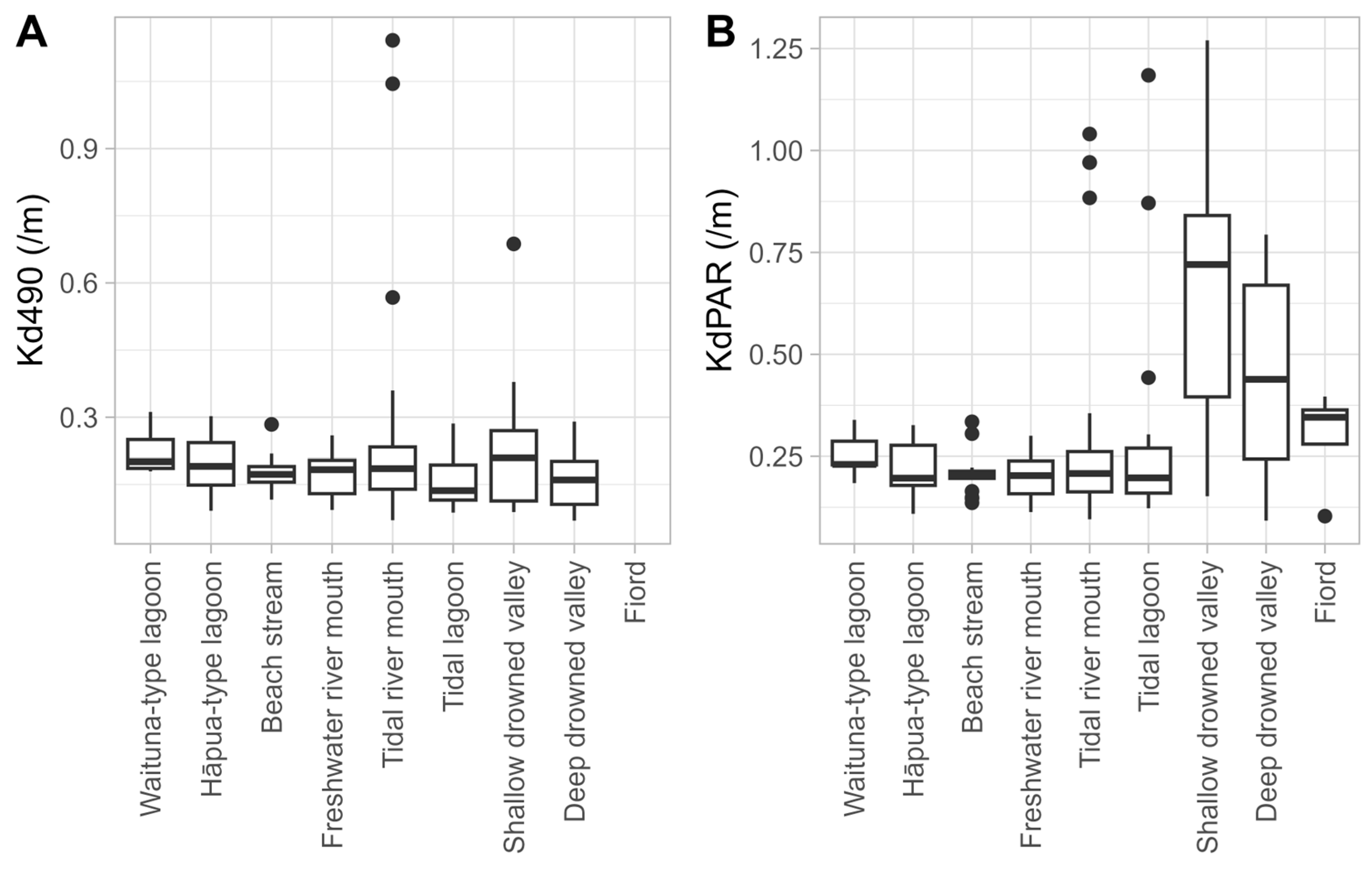
3.2.1. Coastal Hydrosystem Influences

Both assessments showed significant differences in the K_d mean between coastal hydrosystem classes (Figure 6). A notable feature was the high K_d values at river mouths that discharge into shallow drowned valleys, consistent with the influence of sediment retention and resuspension effects in these confined and relatively shallow environments. This was most evident in the K_dPAR results, in which the K_d (mean = 0.67 m⁻¹) differed significantly from all other hydrosystem classes except for Waituna-type lagoons (p < 0.001) in the pairwise comparisons (see Appendix A for descriptions of these New Zealand hydrosystem classes). Despite also returning the highest value in the K_d490 results (mean = 0.24 m⁻¹), the shallow drowned valleys were not significantly different from the other hydrosystem classes.

A comparison of the K_dPAR and K_d490 results shows several major differences in the relationships between classes, including a relatively high K_d490 at Waituna-type lagoons, tidal river mouths, and hāpua-type lagoons that was not seen in the K_dPAR observations (Figure 6). Similar results were also found at other sampling radii (Supplementary Material Figure S1), suggesting that apparent differences between sites were influenced by attributes of the source data within the range of coastal surface water areas that we sampled (up to 505 km² with a 25 km radius). Although these discrepancies can be partly explained by the low level of replication within some of the hydrosystem classes (e.g., n = 6 for Waituna-type lagoons and fiords), the smaller sampling units also returned far fewer valid samples (Figure 5C,D).

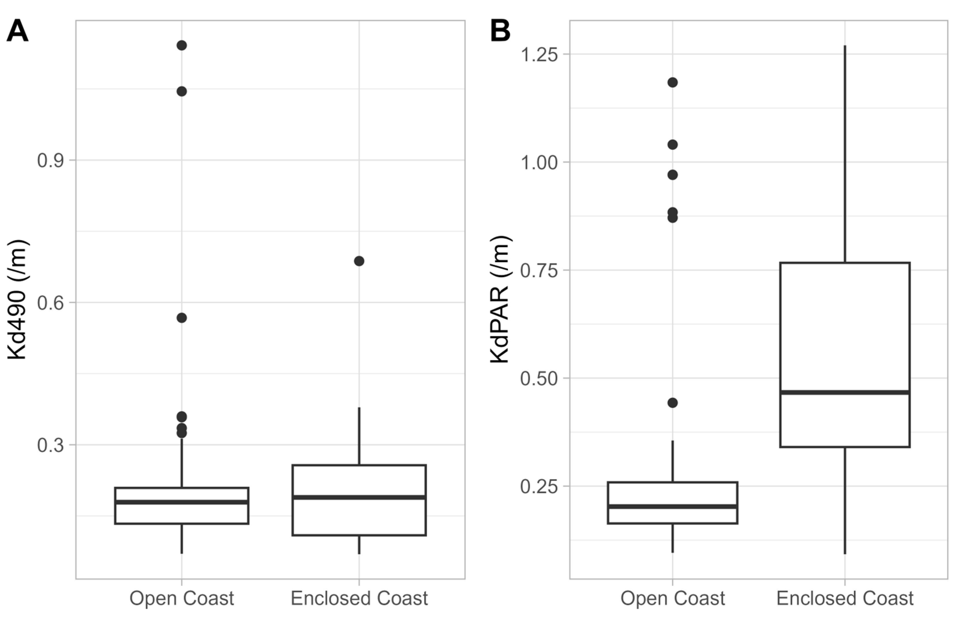
3.2.2. Coastline Geometry

Based on the hydrosystem analysis and morphological similarities in the coastline geometry of shallow drowned valleys, deep drowned valleys, and fiords (i.e., having incised features relative to open coastlines), we classified the sampling units into two coastline geometry classes that separate the ‘open coast’ from the ‘enclosed coast’ river mouth environments. For both data products, the enclosed coasts returned higher K_d values at all radii (Supplementary Material Figure S2) as illustrated for a 10 km radius (Figure 7). However, the difference in the ESA 4 km K_d490 mean values (which were 20% higher than open coasts) was much less pronounced than for the SCENZ 500 m K_dPAR values (which were 250% higher than open coasts), indicating better discrimination using the higher-resolution data source. Pairwise tests showed no significant difference in the ESA 4 km data (p = 0.912) and a highly significant difference (p < 0.001) in the SCENZ 500 m data.

3.3. Case Studies

The case studies in this section present results from three example applications of the river radii framework stratified by coastline geometry using a 10 km sampling radius and the SCENZ 500 m K_dPAR product as the highest-resolution data source. For each case, the differences are also evaluated for the central tendency and also extreme event metrics as represented by lower or higher (e.g., 10th and 90th) percentiles of K_d values over the time series.

3.3.1. Influence of Stream Order and Catchment

On open coasts, the 10th and 50th percentile (median) K_dPAR values increased consistently with higher stream orders, and similarly at the 90th percentile with the exception of stream order 8 which returned slightly lower values than stream order 7 (Figure 8A). Across all stream order classes, the 90th percentile K_dPAR was up to 200% higher than the median value, providing an indication of the effect of extreme events. Differences between stream orders were significant between 5^th and 7^th order streams at both the 50th (p = 0.043) and 90th percentiles (p = 0.011).

On enclosed coasts, there were no significant differences between stream orders and no obvious relationship between stream order and K_dPAR, consistent with the catchment signature being obscured by sediment retention and resuspension effects at these river mouths. The same pattern is also evident in the relationship between K_dPAR and catchment size for the same set of rivers (Supplementary Material Figure S3).

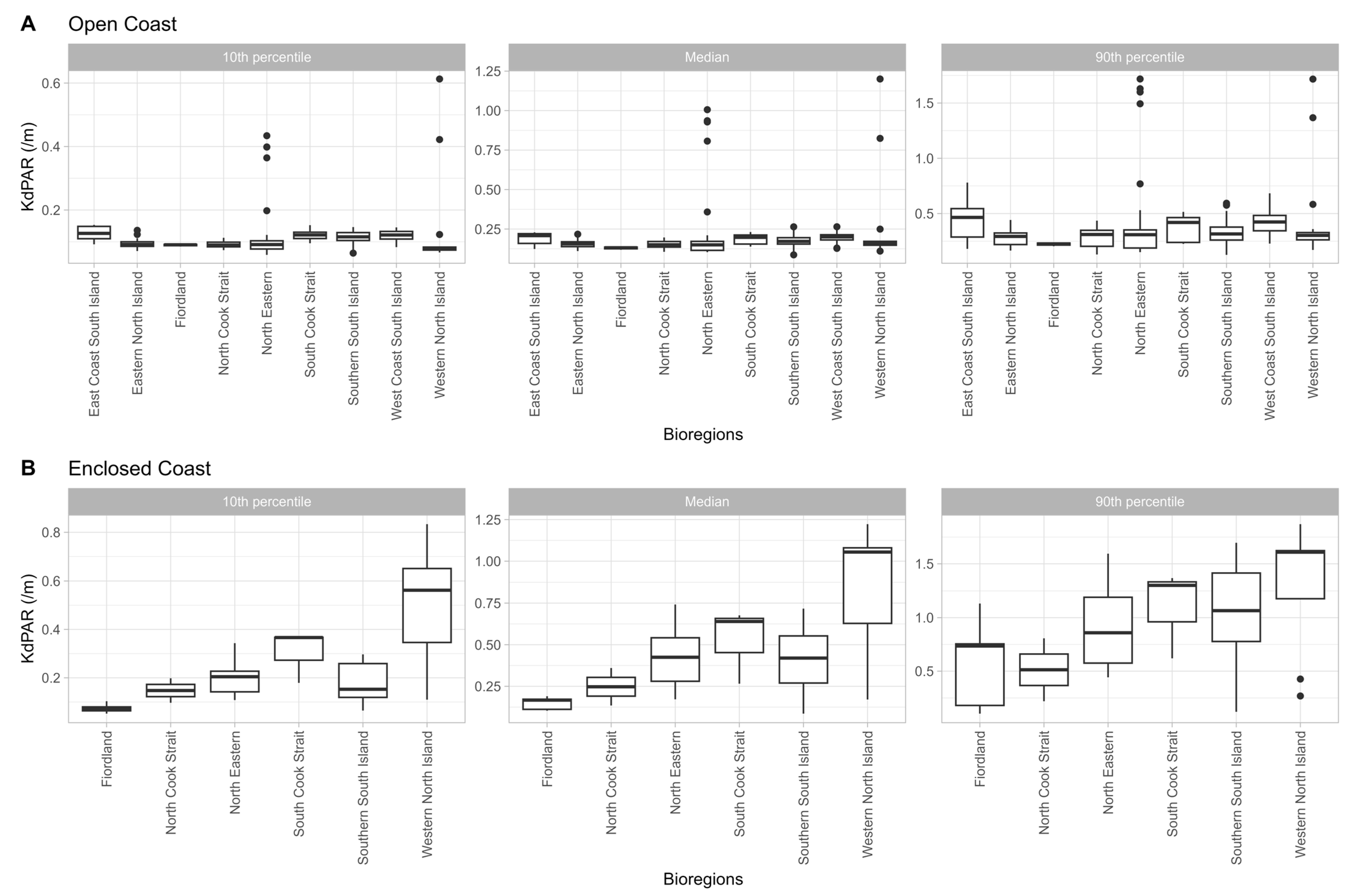
3.3.2. Differences Across Marine Bioregions

Interactions between K_dPAR values, coastline geometry classes, and marine bioregions provide an indication of potential issues associated with the impacts of light limitations on characteristic marine biota (Figure 9). The most striking trends are the markedly higher K_dPAR values observed on enclosed coasts in some bioregions, particularly the Western North Island and South Cook Strait (Figure 9B). On the open coast, the situation is much different, with much lower K_d values in most bioregions. However, the presence of outliers with high K_d values (being individual rivers) on open coasts in the North Eastern and Western North Island bioregions is notable.

For open coasts, the pairwise comparisons also showed statistically significant differences in the median K_dPAR between the South Island West Coast and Eastern North Island, North Cook Strait, and Fiordland bioregions (p < 0.05). At the 90th percentile, a slightly different pattern emerges with significant differences between the South Island West Coast and Eastern North Island, North Cook Strait, and North Eastern bioregions (p < 0.01). However, the highest K_d values were found in the East Coast South Island bioregion, likely reflecting the influence of major alpine rivers passing through erodable terrain. Interestingly, there were no significant differences between bioregions for the enclosed coast river mouths at these percentiles. Instead, however, significant differences were found at the 10th percentile, which are associated with periods of low river flow. This demonstrates that assessing a selection of percentiles offers opportunities to characterise changes and differences between sites under a range of conditions as discussed further in Section 4.4.

Other similar comparisons that can be explored include differences across local government jurisdictions (Supplementary Material Figure S4). While being broadly consistent with patterns across marine bioregions, differences between these anthropogenically-defined areas also highlight important challenges. For example, open coast river mouths in the Auckland region showed noticeably higher K_dPAR values than other regions (Supplementary Material Figure S4).

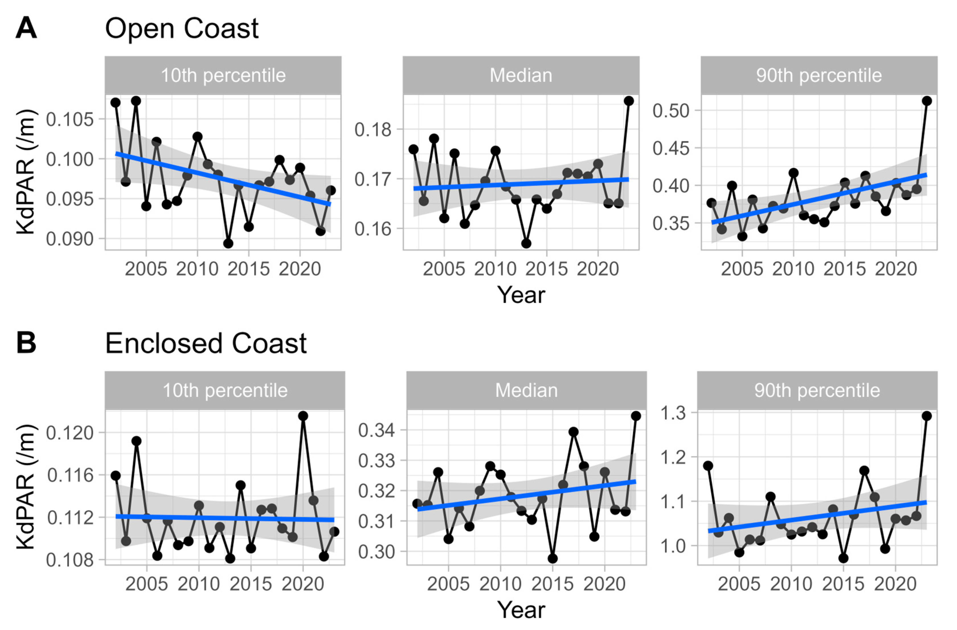
3.3.3. Remote Monitoring of Environmental Changes

A key application for predefined and consistently monitored sampling frameworks is the detection of environmental changes. In this case study, we illustrate applications of the river radii framework to assess time series of SRS metrics across groups of rivers (e.g., national and regional) or at the scale of individual river mouths. For these analyses, we took advantage of the historical period covered by the SCENZ 500 m K_dPAR product and present an evaluation of changes over the 21-year period from July 2002 to August 2023. Figure 10 shows the time series of yearly averaged K_dPAR values across all 226 rivers based on daily data. A visual inspection of the time series shows that these apparent trends are more pronounced on open coasts (Figure 10). The K_d values generally declined at the 10th percentile but increased at the 90th percentile over the period. On open coasts, the 90th percentile trend was significant (Sen’s slope 0.002, p = 0.02), and it is markedly influenced by the last data point which reflects several major flood events, particularly those associated with Cyclone Hale and Cyclone Gabrielle in early 2023. Other apparent trends over the time series were not significant at α = 0.05. However, it is relatively simple to disaggregate these results further to investigate trends within focal areas (e.g., marine bioregions or local government regions).

In addition to evaluating differences between various groups of rivers, comparisons may be made at the scale of individual rivers to pinpoint ‘hotspots’ in the metric of interest. As an example, the 21-year mean K_dPAR values retrieved from the 10 km river radii framework range from a low of 0.09 ± 0.06 (std. dev.) at Lords River/Tūtaekawetoweto in the Southland region, to a high of 1.28 ± 0.47 at Topuni River in the Auckland region (Figure 11). Also notable is a strong inflection point in the range of the K_dPAR values for individual rivers (Figure 11A), and 28 rivers with the highest K_d values lie above this point (Figure 11B). Eight of these rivers are found in the Waikato region and another seven in the Auckland region. These highly turbid rivers contribute to the marked differences that were detected in the comparison of local government jurisdictions (Supplementary Material Figure S4). Moreover, these regional differences are apparent at all of the percentiles we tested (10th, 50th, and 90th).

4. Discussion

4.1. Contributions of a Proximity-Based Framework

Remotely sensed estimates of environmental parameters are being increasingly used in water resource management as a cost-effective means of monitoring environmental changes [46]. Many freely available SRS metrics are highly relevant as indicators of potential issues in coastal marine environments [30,31]. There is additional power in linking SRS observations with formal analysis frameworks that can help to investigate spatio-temporal patterns in indicators of desirable conditions or tease out the potential sources of threats and stressors at relevant scales. The river radii framework provides an approach that can facilitate these opportunities in both targeted studies and the routine monitoring of river mouth environments using a wide range of remotely sensed data sources.

Reviews of remote sensing in river mouth and estuarine environments often focus on documenting the opportunities presented by developments in sensor technology and image processing techniques, or on descriptions of the challenges and limitations for future applications of remote sensing approaches [44,73,74]. For example, a review of over 200 papers on the remote sensing of large river deltas and estuaries showcased applications to both the terrestrial and aquatic dimensions of these environments [44]. The spatial basis of the aquatic and land–water interface studies that were featured is indicative of the field and yet comprises a relatively short list of sampling domains consisting of intertidal zones, shoreline change envelopes, and river plume extents, in addition to areas of inundation associated with flood events or the effects of anthropogenic modifications, such as the expansion of ponds for aquaculture [44]. Another recent review of remote sensing approaches for coastal and river delta regions documented a similar range of conceptual sampling units for spatio-temporal analyses with the addition of point locations for studies of tidal anomalies [41]. There is clearly, therefore, scope for increasing the diversity of spatial frameworks that might usefully be applied to the monitoring of river mouth environments, especially when it is desirable to monitor many sites concurrently, as is the case with state-of-the environment monitoring programmes.

Within the environmental monitoring literature, the use of sampling designs based on radial buffers is primarily found in the fields of urban geography (e.g., [75]) and pollution studies (e.g., [76]). However, there are very few reported applications to water resource management with most of the contaminant-oriented studies being concerned with air pollution from point sources (e.g., [77]). Notable exceptions include studies of groundwater pollution (e.g., [78]), and a study of the relationships between in situ water quality measurements and land use or land cover (LULC) variables in the surrounding landscape as sampled using radial buffers centred on the water quality monitoring locations [79].

Another approach with some similarities to our proximity-based sampling framework involves feature-based sampling. This is common in studies of semi-enclosed water bodies such as harbours and estuaries, where it is relatively intuitive to manually delineate the extent of the water feature using adjacent landscape features such as headlands (e.g., [80]) or by applying image processing techniques to identify the ‘enclosed’ water surface area (e.g., [81]). Similarly, a feature-based approach forms the basis for the remote sensing of planform morphometrics or water quality parameters in large rivers where the water surface area can be extracted (e.g., [82,83,84]). Nonetheless, these approaches do not yield a spatially consistent sampling unit for the purpose of observing differences in the characteristics of fluvial discharges in coastal environments since these larger features vary considerably in their spatial dimensions. In comparison, the utility of our framework can clearly be seen at the sub-feature scale in several harbours and drowned valleys where the river signature is clearly visible as an area of more turbid water proximal to the river mouth (e.g., Whangaroa Harbour, Figure 2C).

As the above discussion illustrates, the consistent spatial basis of the river radii framework is a key strength in comparison to other approaches. In addition, its inherent flexibility when selecting an appropriate sampling unit size offers an approach that is generally applicable to a wide range of river mouth types and coastal receiving environments. Furthermore, nested analyses of multiple radii can support sensitivity analysis of apparent effects and provides a means of investigating the spatial extent of river influences. Analogous examples of this approach in other fields include the use of radial buffers of different sizes for sensitivity analysis in studies of transportation geography (e.g., [85]). Somewhat coincidently, such studies also use the language of ‘catchments’, which, in this case, refer to the areas that are sampled.

The distinguishing features of the river radii framework also naturally lead to a consideration of its differences from, and complementarity to river plume tracking as a well-established approach for the monitoring of fluvial influences on coastal environments. River plume studies typically focus on the investigation of plume dynamics to understand the mechanisms that drive their formation and characteristics (e.g., [19,28,86,87]) and the tracking of individual plumes can also provide insights for the characterisation of problematic land use or river management practices (e.g., [21,88]). However, limitations arise from the focus on delineating areas of high turbidity [18]. Consequently, many of the insights gained are specific to the underlying concept of an optically differentiated plume that is defined as the area of interest. Unsurprisingly, river discharge is often identified as the primary forcing factor that drives variation in the plume response even though wind and tidal forcing, ocean circulation patterns, and retention times are also frequently identified as further influences [29,89,90].

A key difference between plume modelling and the river radii approach is the spatial basis of the sampling unit, with the proximity-based sampling approach having a greater focus on supporting spatio-temporal comparisons within a pre-defined sampling area. This provides a different view of environmental change that complements the spatial extent and severity metrics that are typical of plume tracking studies. The two approaches can also be combined in investigations of plume impacts within various radii of interest for one or more rivers. However, a particular strength of the river radii approach is its lack of reliance on the delineation of a plume, which supports a wider range of monitoring objectives in river mouth environments.

4.2. Optimum Sampling Radius

A key finding for the development of a proximity-based sampling framework for SRS data is the identification of an optimum sampling radius. Our results demonstrate the existence of a lower limit to the size of sampling units that are efficient for applications to time series analyses. This arises from an observed increase in variance at small radii that is most likely explained by the proportionally higher reductions in the number of observations that are available for analysis following cloud filtering and validation procedures. Another contributing factor relates to the land ‘glow’ effect of near infra-red radiation that confounds ocean colour retrievals from nearshore pixels, adding to the apparent variation across pixels that are expected to have comparable surface water reflectance [91,92]. These source data characteristics penalise the nearshore areas by reducing the number of valid images for data retrieval within individual scenes and over time series, and by imposing greater measurement error and variability on nearshore pixels. For example, there was almost a three-fold increase in the post-validation sample size between the 1 and 20 km sampling radii in the K_dPAR analyses (Figure 5).

Conversely, these effects were observed as a notable drop in variance beyond 5 km in the 500 m K_dPAR analyses and a similar, though less apparent, trend with increasing radii in the 4 km K_d490 analyses, in which larger radii were used (Figure 5). The high variance threshold at 5 km observed in this study using 500 m resolution data also suggests that there is a ‘sweet spot’ that balances the variance found in small sampling radii with the reduced specificity to individual rivers of larger sampling units, particularly those that capture the influence of adjacent rivers (e.g., nearby river plumes). For both SRS products, we believe that the optimum radius lies in the 5–10 km range and suggest that similar principles might apply to other SRS data sources.

4.3. Effects of Data Resolution and Coastline Geometry

Our results also illustrate the significant influence of source data resolution on the detection power and interpretation of SRS analyses. In this study, such effects were particularly evident in the difference between open and enclosed coast K_d values that were obtained from each data product, with the 500 m product detecting high K_d values on enclosed coasts in comparison to open coasts, which was generally not observed in the 4 km product. The main characteristic of this discrepancy is the larger pixel size’s apparent inability to resolve high K_d conditions on enclosed coasts, with the open and enclosed coast results showing similar K_d mean and median values over the 10-year period we analysed (Figure 7). These findings are particularly relevant and transferable to the monitoring of changes in the vicinity of land or ice in other situations in which SRS products for surface water observations must be clipped to avoid the inclusion of non-target pixels [93]. Spatial resolution (pixel size) has a strong bearing on the overall area of surface water that cannot be effectively observed due to the clipping (removal) of water boundary pixels that contain the confounding elements (i.e., land or ice). The takeaway principles of this study that may be applied to other remote sensing contexts include a need to be cognizant of the limitations of coarse spatial resolution data for studies of nearshore environments. These findings also suggest that improving the availability of higher resolution data that are also temporally dense will be particularly beneficial for coastal monitoring applications.

Another notable finding of our comparative analyses was the identification of coastline geometry as a significant influence on the number of observations that are available for SRS analyses in nearshore environments. This is likely due to the greater potential for convoluted coastlines to intersect with individual pixel boundaries, resulting in the removal of those pixels. This effect was apparent in data retrieval from both data sources (e.g., a 40% reduction of valid images for the 4 km product and a 52% reduction for the 500 m product over the same 10-year period) (Supplementary Material Figure S5). Moreover, these findings illustrate the benefit of using a stratified sampling design to address the effects of coastline geometry and highlight the important influence of this variable. We recommend this as a standard component of SRS sampling frameworks for nearshore environments, particularly when comparisons between sites are desired. Our simple two-class coastline geometry classification provides a pragmatic option for achieving this in a manner that is both defensible and preserves sufficient sample numbers in each stratum. However, there may also be other alternative classifications that achieve this objective or are perhaps better suited for other geographical scales and contexts. We identify this as a key topic for further consideration and research.

4.4. Applications and Future Directions

This study demonstrates some of the potential applications and practical advantages of the river radii framework for environmental monitoring in river mouth environments using freely available SRS data products. We do note, however, that further validation of this approach is needed to test its applicability to a wider range of environmental contexts and management questions. Although it is relatively easy to track changes at a single site, there are considerable opportunities to leverage comparative analyses that evaluate differences between sites or across gradients as an approach to understanding the factors that drive change in observable outcomes. Comparative analyses based on selected percentiles across time series of interest are a practical way of evaluating the available SRS data in a consistent format that can provide a useful indicator of both average and extreme conditions. Diagnostic applications include investigations of the prevalence and potential sources of stressors on coastal environments, which are especially needed to address threats from land use in upstream catchments [94]. Other potential applications include the identification of restoration opportunities which requires knowledge of the drivers of degradation [95], and the prioritisation of locations for area-based management approaches such as protected areas, OECMs, or other spatial planning initiatives that can improve environmental outcomes [96,97].

The river radii approach provides a framework that supports these objectives while being complementary to plume tracking studies and readily applicable to a wide range of remotely sensed data sources. Some of the standardised metrics that can be derived include time-averaged statistics at selected percentiles that are indicative of low, high, and average conditions, time series trends, and cumulative intensity or change metrics for event-based phenomena such as storms and marine heatwaves. It can assist investigations of land-to-sea connectivity through its comparative basis and is well suited to the development of cost-effective approaches for river mouth monitoring at local, national, and global scales.

References

1. Cicin-Sain, B.; Knecht, R. Integrated Coastal and Ocean Management: Concepts and Practices; Island Press: Washington, DC, USA, 2013. [Google Scholar]
2. Côté, I.M.; Darling, E.S.; Brown, C.J. Interactions among ecosystem stressors and their importance in conservation. Proc. R. Soc. B Biol. Sci. 2016, 283, 20152592. [Google Scholar] [CrossRef] [PubMed]
3. Crain, C.M.; Kroeker, K.; Halpern, B.S. Interactive and cumulative effects of multiple human stressors in marine systems. Ecol. Lett. 2008, 11, 1304–1315. [Google Scholar] [CrossRef] [PubMed]
4. Álvarez-Romero, J.G.; Pressey, R.L.; Ban, N.C.; Vance-Borland, K.; Willer, C.; Klein, C.J.; Gaines, S.D. Integrated land-sea conservation planning: The missing links. Annu. Rev. Ecol. Evol. Syst. 2011, 42, 381–409. [Google Scholar] [CrossRef]
5. Polasky, S.; Carpenter, S.R.; Folke, C.; Keeler, B. Decision-making under great uncertainty: Environmental management in an era of global change. Trends Ecol. Evol. 2011, 26, 398–404. [Google Scholar] [CrossRef]
6. Andersen, J.H.; Al-Hamdani, Z.; Harvey, E.T.; Kallenbach, E.; Murray, C.; Stock, A. Relative impacts of multiple human stressors in estuaries and coastal waters in the North Sea–Baltic Sea transition zone. Sci. Total Environ. 2020, 704, 135316. [Google Scholar] [CrossRef]
7. Halpern, B.S.; Frazier, M.; Afflerbach, J.; Lowndes, J.S.; Micheli, F.; O’Hara, C.; Scarborough, C.; Selkoe, K.A. Recent pace of change in human impact on the world’s ocean. Sci. Rep. 2019, 9, 11609. [Google Scholar] [CrossRef]
8. Hodapp, D.; Roca, I.T.; Fiorentino, D.; Garilao, C.; Kaschner, K.; Kesner-Reyes, K.; Schneider, B.; Segschneider, J.; Kocsis, Á.T.; Kiessling, W.; et al. Climate change disrupts core habitats of marine species. Glob. Change Biol. 2023, 29, 3304–3317. [Google Scholar] [CrossRef]
9. IPCC. Climate Change 2023: Synthesis Report. Contribution of Working Groups I, II and III to the Sixth Assessment Report of the Intergovernmental Panel on Climate Change; IPCC: Geneva, Switzerland, 2023. [Google Scholar]
10. Abell, R. Conservation biology for the biodiversity crisis: A freshwater follow-up. Conserv. Biol. 2002, 16, 1435–1437. [Google Scholar] [CrossRef]
11. Halpern, B.S.; Walbridge, S.; Selkoe, K.A.; Kappel, C.V.; Micheli, F.; D’Agrosa, C.; Bruno, J.F.; Casey, K.S.; Ebert, C.; Fox, H.E.; et al. A global map of human impact on marine ecosystems. Science 2008, 319, 948–952. [Google Scholar] [CrossRef]
12. Albert, J.S.; Destouni, G.; Duke-Sylvester, S.M.; Magurran, A.E.; Oberdorff, T.; Reis, R.E.; Winemiller, K.O.; Ripple, W.J. Scientists’ warning to humanity on the freshwater biodiversity crisis. AmBio 2020, 50, 85–94. [Google Scholar] [CrossRef]
13. Barbier, E.B.; Hacker, S.D.; Kennedy, C.; Koch, E.W.; Stier, A.C.; Silliman, B.R. The value of estuarine and coastal ecosystem services. Ecol. Monogr. 2011, 81, 169–193. [Google Scholar] [CrossRef]
14. Lopez-Rivas, J.D.; Cardenas, J.-C. What is the economic value of coastal and marine ecosystem services? A systematic literature review. Mar. Policy 2024, 161, 106033. [Google Scholar] [CrossRef]
15. Seitz, R.D.; Wennhage, H.; Bergström, U.; Lipcius, R.N.; Ysebaert, T. Ecological value of coastal habitats for commercially and ecologically important species. ICES J. Mar. Sci. 2013, 71, 648–665. [Google Scholar] [CrossRef]
16. Jonsson, P.R.; Hammar, L.; Wåhlström, I.; Pålsson, J.; Hume, D.; Almroth-Rosell, E.; Mattsson, M. Combining seascape connectivity with cumulative impact assessment in support of ecosystem-based marine spatial planning. J. Appl. Ecol. 2021, 58, 576–586. [Google Scholar] [CrossRef]
17. Foley, M.M.; Mease, L.A.; Martone, R.G.; Prahler, E.E.; Morrison, T.H.; Murray, C.C.; Wojcik, D. The challenges and opportunities in cumulative effects assessment. Environ. Impact Assess. Rev. 2017, 62, 122–134. [Google Scholar] [CrossRef]
18. Álvarez-Romero, J.G.; Devlin, M.; Teixeira da Silva, E.; Petus, C.; Ban, N.C.; Pressey, R.L.; Kool, J.; Roberts, J.J.; Cerdeira-Estrada, S.; Wenger, A.S.; et al. A novel approach to model exposure of coastal-marine ecosystems to riverine flood plumes based on remote sensing techniques. J. Environ. Manag. 2013, 119, 194–207. [Google Scholar] [CrossRef]
19. Restrepo, J.D.; Park, E.; Aquino, S.; Latrubesse, E.M. Coral reefs chronically exposed to river sediment plumes in the southwestern Caribbean: Rosario Islands, Colombia. Sci. Total Environ. 2016, 553, 316–329. [Google Scholar] [CrossRef]
20. Devlin, M.J.; McKinna, L.W.; Álvarez-Romero, J.G.; Petus, C.; Abott, B.; Harkness, P.; Brodie, J. Mapping the pollutants in surface riverine flood plume waters in the Great Barrier Reef, Australia. Mar. Pollut. Bull. 2012, 65, 224–235. [Google Scholar] [CrossRef]
21. Petus, C.; da Silva, E.T.; Devlin, M.; Wenger, A.S.; Álvarez-Romero, J.G. Using MODIS data for mapping of water types within river plumes in the Great Barrier Reef, Australia: Towards the production of river plume risk maps for reef and seagrass ecosystems. J. Environ. Manag. 2014, 137, 163–177. [Google Scholar] [CrossRef]
22. Beck, M.W.; Heck, K.L.; Able, K.W.; Childers, D.L.; Eggleston, D.B.; Gillanders, B.M.; Halpern, B.; Hays, C.G.; Hoshino, K.; Minello, T.J.; et al. The identification, conservation, and management of estuarine and marine nurseries for fish and invertebrates: A better understanding of the habitats that serve as nurseries for marine species and the factors that create site-specific variability in nursery quality will improve conservation and management of these areas. Bioscience 2001, 51, 633–641. [Google Scholar] [CrossRef]
23. Elliott, M.; Whitfield, A.K. Challenging paradigms in estuarine ecology and management. Estuar. Coast. Shelf Sci. 2011, 94, 306–314. [Google Scholar] [CrossRef]
24. Orchard, S. Cultural ecosystem services and the natural capital of nature-based recreation and fisheries. In Routledge Handbook of Cultural Ecosystem Services; McElwee, P., Ed.; Routledge: London, UK, 2025. [Google Scholar]
25. Schiel, D.R.; Howard-Williams, C. Controlling inputs from the land to sea: Limit-setting, cumulative impacts and ki uta ki tai. Mar. Freshw. Res. 2016, 67, 57–64. [Google Scholar] [CrossRef]
26. Kroon, F.J.; Kuhnert, P.M.; Henderson, B.L.; Wilkinson, S.N.; Kinsey-Henderson, A.; Abbott, B.; Brodie, J.E.; Turner, R.D.R. River loads of suspended solids, nitrogen, phosphorus and herbicides delivered to the Great Barrier Reef lagoon. Mar. Pollut. Bull. 2012, 65, 167–181. [Google Scholar] [CrossRef] [PubMed]
27. Geyer, W.R.; Hill, P.S.; Kineke, G.C. The transport, transformation and dispersal of sediment by buoyant coastal flows. Cont. Shelf Res. 2004, 24, 927–949. [Google Scholar] [CrossRef]
28. Restrepo, J.D.; Zapata, P.; Díaz, J.M.; Garzón-Ferreira, J.; García, C.B. Fluvial fluxes into the Caribbean Sea and their impact on coastal ecosystems: The Magdalena River, Colombia. Glob. Planet. Change 2006, 50, 33–49. [Google Scholar] [CrossRef]
29. Moreno-Madriñán, M.J.; Rickman, D.L.; Ogashawara, I.; Irwin, D.E.; Ye, J.; Al-Hamdan, M.Z. Using remote sensing to monitor the influence of river discharge on watershed outlets and adjacent coral Reefs: Magdalena River and Rosario Islands, Colombia. Int. J. Appl. Earth Obs. Geoinf. 2015, 38, 204–215. [Google Scholar] [CrossRef]
30. Yang, H.; Kong, J.; Hu, H.; Du, Y.; Gao, M.; Chen, F. A review of remote sensing for water quality retrieval: Progress and challenges. Remote Sens. 2022, 14, 1770. [Google Scholar] [CrossRef]
31. McCarthy, M.J.; Colna, K.E.; El-Mezayen, M.M.; Laureano-Rosario, A.E.; Méndez-Lázaro, P.; Otis, D.B.; Toro-Farmer, G.; Vega-Rodriguez, M.; Muller-Karger, F.E. Satellite remote sensing for coastal management: A review of successful applications. Environ. Manag. 2017, 60, 323–339. [Google Scholar] [CrossRef]
32. Bhargava, A.; Sachdeva, A.; Sharma, K.; Alsharif, M.H.; Uthansakul, P.; Uthansakul, M. Hyperspectral imaging and its applications: A review. Heliyon 2024, 10, e33208. [Google Scholar] [CrossRef]
33. Sharaf El Din, E.; Yun, Z.; and Suliman, A. Mapping concentrations of surface water quality parameters using a novel remote sensing and artificial intelligence framework. Int. J. Remote Sens. 2017, 38, 1023–1042. [Google Scholar] [CrossRef]
34. Jaywant, S.A.; Arif, K.M. Remote sensing techniques for water quality monitoring: A review. Sensors 2024, 24, 8041. [Google Scholar] [CrossRef] [PubMed]
35. Mohseni, F.; Saba, F.; Mirmazloumi, S.M.; Amani, M.; Mokhtarzade, M.; Jamali, S.; Mahdavi, S. Ocean water quality monitoring using remote sensing techniques: A review. Mar. Environ. Res. 2022, 180, 105701. [Google Scholar] [CrossRef] [PubMed]
36. Gattuso, J.P.; Gentili, B.; Antoine, D.; Doxaran, D. Global distribution of photosynthetically available radiation on the seafloor. Earth Syst. Sci. Data 2020, 12, 1697–1709. [Google Scholar] [CrossRef]
37. Kim, Y.J.; Daehyeon, H.; Eunna, J.; Jungho, I.; and Sung, T. Remote sensing of sea surface salinity: Challenges and research directions. GIScience Remote Sens. 2023, 60, 2166377. [Google Scholar] [CrossRef]
38. Merchant, C.J.; Embury, O.; Bulgin, C.E.; Block, T.; Corlett, G.K.; Fiedler, E.; Good, S.A.; Mittaz, J.; Rayner, N.A.; Berry, D.; et al. Satellite-based time-series of sea-surface temperature since 1981 for climate applications. Sci. Data 2019, 6, 223. [Google Scholar] [CrossRef]
39. Minnett, P.J.; Alvera-Azcárate, A.; Chin, T.M.; Corlett, G.K.; Gentemann, C.L.; Karagali, I.; Li, X.; Marsouin, A.; Marullo, S.; Maturi, E.; et al. Half a century of satellite remote sensing of sea-surface temperature. Remote Sens. Environ. 2019, 233, 111366. [Google Scholar] [CrossRef]
40. Vos, K.; Splinter, K.D.; Palomar-Vázquez, J.; Pardo-Pascual, J.E.; Almonacid-Caballer, J.; Cabezas-Rabadán, C.; Kras, E.C.; Luijendijk, A.P.; Calkoen, F.; Almeida, L.P.; et al. Benchmarking satellite-derived shoreline mapping algorithms. Commun. Earth Environ. 2023, 4, 345. [Google Scholar] [CrossRef]
41. Zhao, Q.; Pan, J.; Devlin, A.T.; Tang, M.; Yao, C.; Zamparelli, V.; Falabella, F.; Pepe, A. On the exploitation of remote sensing technologies for the monitoring of coastal and river delta regions. Remote Sens. 2022, 14, 2384. [Google Scholar] [CrossRef]
42. Xu, N.; Ma, Y. Satellite remote sensing based coastal bathymetry inversion. In Current Trends in Estuarine and Coastal Dynamics, Wang, X.H., Qiao, L., Mitchell, S., Elliott, M., Eds.; Elsevier: Amsterdam, The Netherlands, 2024; Volume 4, pp. 45–73. [Google Scholar]
43. Jawak, S.; Vadlamani, S.; Luis, A. A synoptic review on deriving bathymetry information using remote sensing technologies: Models, methods and comparisons. Adv. Remote Sens. 2015, 4, 147–162. [Google Scholar] [CrossRef]
44. Kuenzer, C.; Heimhuber, V.; Huth, J.; Dech, S. Remote sensing for the quantification of land surface dynamics in large river delta regions—A review. Remote Sens. 2019, 11, 1985. [Google Scholar] [CrossRef]
45. Raffa, F.; Alberico, I.; Serafino, F. X-band radar system to detect bathymetric changes at river mouths during storm surges: A case study of the Arno River. Sensors 2022, 22, 9415. [Google Scholar] [CrossRef] [PubMed]
46. Sheffield, J.; Wood, E.F.; Pan, M.; Beck, H.; Coccia, G.; Serrat-Capdevila, A.; Verbist, K. Satellite remote sensing for water resources management: Potential for supporting sustainable development in data-poor regions. Water Resour. Res. 2018, 54, 9724–9758. [Google Scholar] [CrossRef]
47. Adjovu, G.E.; Stephen, H.; James, D.; Ahmad, S. Overview of the application of remote sensing in effective monitoring of water quality parameters. Remote Sens. 2023, 15, 1938. [Google Scholar] [CrossRef]
48. Schaeffer, B.A.; Schaeffer, K.G.; Keith, D.; Lunetta, R.S.; Conmy, R.; Gould, R.W. Barriers to adopting satellite remote sensing for water quality management. Int. J. Remote Sens. 2013, 34, 7534–7544. [Google Scholar] [CrossRef]
49. Tait, L.W.; Orchard, S.; Schiel, D.R. Missing the forest and the trees: Utility, limits and caveats for drone imaging of coastal marine ecosystems. Remote Sens. 2021, 13, 3136. [Google Scholar] [CrossRef]
50. Lee, Z.-P. A model for the diffuse attenuation coefficient of downwelling irradiance. J. Geophys. Res. 2005, 110, C02016. [Google Scholar] [CrossRef]
51. Myint, S.W.; Walker, N.D. Quantification of surface suspended sediments along a river dominated coast with NOAA AVHRR and SeaWiFS measurements: Louisiana, USA. Int. J. Remote Sens. 2002, 23, 3229–3249. [Google Scholar] [CrossRef]
52. Kirk, J.T.O. Light and Photosynthesis in Aquatic Ecosystems, 2nd ed.; Cambridge University Press: Cambridge, UK, 1994. [Google Scholar]
53. Snelder, T.H.; Biggs, B.J.F. Multi-scale river environment classification for water resources management. J. Am. Water Resour. Assoc. 2002, 38, 1225–1240. [Google Scholar] [CrossRef]
54. NIWA. REC2 (River Environment Classification, v2.5). 2019. Available online: https://niwa.co.nz/freshwater/river-environment-classification-2 (accessed on 24 February 2025).
55. Snelder, T.; Biggs, B.; Weatherhead, M. New Zealand River Environment Classification User Guide. 2010. Available online: https://environment.govt.nz/assets/publications/acts-regs-and-policy-statements/rec-user-guide-2010.pdf (accessed on 24 February 2025).
56. Kirk, R.M. River-beach interaction on mixed sand and gravel coasts: A geomorphic model for water resource planning. Appl. Geogr. 1991, 11, 267–287. [Google Scholar] [CrossRef]
57. Measures, R.J.; Hart, D.E.; Cochrane, T.A.; Hicks, D.M. Processes controlling river-mouth lagoon dynamics on high-energy mixed sand and gravel coasts. Mar. Geol. 2020, 420, 106082. [Google Scholar] [CrossRef]
58. Strahler, A.N. Quantitative analysis of watershed geomorphology. Eos Trans. Am. Geophys. Union 1957, 38, 913–920. [Google Scholar] [CrossRef]
59. Memon, P.A.; Perkins, H.C. Environmental Planning and Management in New Zealand; Dunmore Press: Palmerston North, New Zealand, 2000. [Google Scholar]
60. Orchard, S. Implications of the New Zealand Coastal Policy Statement 2010 for New Zealand Communities; Environment & Conservation Organisations of New Zealand: Wellington, New Zealand, 2011. [Google Scholar]
61. Peart, R. Beyond the tide. In Integrating the Management of New Zealand’s Coasts; Environmental Defence Society: Auckland, New Zealand, 2007. [Google Scholar]
62. Hume, T.M.; Herdendorf, C.E. A geomorphic classification of estuaries and its application to coastal resource management—A New Zealand example. Ocean Shorel. Manag. 1988, 11, 249–274. [Google Scholar] [CrossRef]
63. Hume, T.; Gerbeaux, P.; Hart, D.; Kettles, H.; Neale, D. A Classification of New Zealand’s Coastal Hydrosystems. 2016. Available online: https://environment.govt.nz/publications/a-classification-of-new-zealands-coastal-hydrosystems/ (accessed on 24 February 2025).
64. Sathyendranath, S.; Brewin, R.J.W.; Brockmann, C.; Brotas, V.; Calton, B.; Chuprin, A.; Cipollini, P.; Couto, A.B.; Dingle, J.; Doerffer, R.; et al. An Ocean-Colour Time Series for Use in Climate Studies: The Experience of the Ocean-Colour Climate Change Initiative (OC-CCI). Sensors 2019, 19, 4285. [Google Scholar] [CrossRef]
65. van Oostende, M.; Hieronymi, M.; Krasemann, H.; Baschek, B.; Röttgers, R. Correction of inter-mission inconsistencies in merged ocean colour satellite data. Front. Remote Sens. 2022, 3, 2418. [Google Scholar] [CrossRef]
66. Morel, A.; Huot, Y.; Gentili, B.; Werdell, P.J.; Hooker, S.B.; Franz, B.A. Examining the consistency of products derived from various ocean color sensors in open ocean (Case 1) waters in the perspective of a multi-sensor approach. Remote Sens. Environ. 2007, 111, 69–88. [Google Scholar] [CrossRef]
67. Gall, M.P.; Pinkerton, M.H.; Steinmetz, T.; Wood, S. Satellite remote sensing of coastal water quality in New Zealand. N. Z. J. Mar. Freshw. Res. 2022, 56, 585–616. [Google Scholar] [CrossRef]
68. Ruddick, K.G.; Ovidio, F.; Rijkeboer, M. Atmospheric correction of SeaWiFS imagery for turbid coastal and inland waters. Appl. Opt. 2000, 39, 897–912. [Google Scholar] [CrossRef]
69. Lee, Z.; Carder, K.L.; Arnone, R.A. Deriving inherent optical properties from water color: A multiband quasi-analytical algorithm for optically deep waters. Appl. Opt. 2002, 41, 5755–5772. [Google Scholar] [CrossRef]
70. Lee, Z.; Lubac, B.; Werdell, J.; Arnone, R. An update of the quasi-analytical algorithm (QAA_v5). In International Ocean Color Group Software Report; IOCCG: Halifax, NS, Canada, 2009; pp. 1–9. [Google Scholar]
71. Morel, A.; Gentili, B.; Claustre, H.; Babin, M.; Bricaud, A.; Ras, J.; Tieche, F. Optical properties of the “clearest” natural waters. Limnol. Oceanogr. 2007, 52, 217–229. [Google Scholar] [CrossRef]
72. R Core Team. R: A Language and Environment for Statistical Computing; R Foundation for Statistical Computing: Vienna, Austria, 2024. [Google Scholar]
73. Munasinghe, D.; Cohen, S.; Gadiraju, K. A review of satellite remote sensing techniques of river delta morphology change. Remote Sens. Earth Syst. Sci. 2021, 4, 44–75. [Google Scholar] [CrossRef]
74. Kuenzer, C.; Klein, I.; Ullmann, T.; Georgiou, E.F.; Baumhauer, R.; Dech, S. Remote sensing of river delta inundation: Exploiting the potential of coarse spatial resolution, temporally-dense MODIS time series. Remote Sens. 2015, 7, 8516–8542. [Google Scholar] [CrossRef]
75. Schneider, A.; Mertes, C.M. Expansion and growth in Chinese cities, 1978–2010. Environ. Res. Lett. 2014, 9, 024008. [Google Scholar] [CrossRef]
76. Manjarrez-Domínguez, C.B.; Prieto-Amparán, J.A.; Valles-Aragón, M.C.; Delgado-Caballero, M.D.R.; Alarcón-Herrera, M.T.; Nevarez-Rodríguez, M.C.; Vázquez-Quintero, G.; Berzoza-Gaytan, C.A. Arsenic distribution assessment in a residential area polluted with mining residues. Int. J. Environ. Res. Public Health 2019, 16, 375. [Google Scholar] [CrossRef] [PubMed]
77. Ebisu, K.; Belanger, K.; Bell, M.L. Association between airborne PM2.5 chemical constituents and birth weight—Implication of buffer exposure assignment. Environ. Res. Lett. 2014, 9, 084007. [Google Scholar] [CrossRef]
78. Xiong, Y.; Liu, J.; Yuan, W.; Liu, W.; Ma, S.; Wang, Z.; Li, T.; Wang, Y.; Wu, J. Groundwater contamination risk assessment based on groundwater vulnerability and pollution loading: A case study of typical karst areas in China. Sustainability 2022, 14, 9898. [Google Scholar] [CrossRef]
79. Huang, W.; Mao, J.; Zhu, D.; Lin, C. Impacts of land use and land cover on water quality at multiple buffer-zone scales in a lakeside city. Water 2020, 12, 47. [Google Scholar] [CrossRef]
80. Tao, J.; Hill, P.S. Correlation of remotely sensed surface reflectance with forcing variables in six different estuaries. J. Geophys. Res. Ocean. 2019, 124, 9439–9461. [Google Scholar] [CrossRef]
81. Liu, C.; Gao, J.; Liu, S.; Li, C.; Cheng, Y.; Luo, Y.; Yang, J. Harbor detection in polarimetric SAR images based on context features and reflection symmetry. Remote Sens. 2024, 16, 3079. [Google Scholar] [CrossRef]
82. Nagel, G.W.; Darby, S.E.; Leyland, J. The use of satellite remote sensing for exploring river meander migration. Earth-Sci. Rev. 2023, 247, 104607. [Google Scholar] [CrossRef]
83. Zhou, Y.; Dong, J.; Xiao, X.; Xiao, T.; Yang, Z.; Zhao, G.; Zou, Z.; Qin, Y. Open surface water mapping algorithms: A comparison of water-related spectral indices and sensors. Water 2017, 9, 256. [Google Scholar] [CrossRef]
84. Zhang, W.; Hu, B.; Brown, G.S. Automatic surface water mapping using polarimetric SAR data for long-term change detection. Water 2020, 12, 872. [Google Scholar] [CrossRef]
85. Liu, X.; Chen, X.; Tian, M.; De Vos, J. Effects of buffer size on associations between the built environment and metro ridership: A machine learning-based sensitive analysis. J. Transp. Geogr. 2023, 113, 103730. [Google Scholar] [CrossRef]
86. Mendes, R.; Vaz, N.; Fernández-Nóvoa, D.; da Silva, J.C.B.; deCastro, M.; Gómez-Gesteira, M.; Dias, J.M. Observation of a turbid plume using MODIS imagery: The case of Douro estuary (Portugal). Remote Sens. Environ. 2014, 154, 127–138. [Google Scholar] [CrossRef]
87. Ondrusek, M.; Stengel, E.; Kinkade, C.S.; Vogel, R.L.; Keegstra, P.; Hunter, C.; Kim, C. The development of a new optical total suspended matter algorithm for the Chesapeake Bay. Remote Sens. Environ. 2012, 119, 243–254. [Google Scholar] [CrossRef]
88. Álvarez-Romero, J.G.; Pressey, R.L.; Ban, N.C.; Brodie, J. Advancing land-sea conservation planning: Integrating modelling of catchments, land-use change, and river plumes to prioritise catchment management and protection. PLoS ONE 2015, 10, e0145574. [Google Scholar] [CrossRef]
89. Horner-Devine, A.R.; Hetland, R.D.; MacDonald, D.G. Mixing and transport in coastal river plumes. Annu. Rev. Fluid Mech. 2015, 47, 569–594. [Google Scholar] [CrossRef]
90. Torregroza-Espinosa, A.C.; Restrepo, J.C.; Correa-Metrio, A.; Hoyos, N.; Escobar, J.; Pierini, J.; Martínez, J.-M. Fluvial and oceanographic influences on suspended sediment dispersal in the Magdalena River Estuary. J. Mar. Syst. 2020, 204, 103282. [Google Scholar] [CrossRef]
91. Santer, R.; Schmechtig, C. Adjacency effects on water surfaces: Primary scattering approximation and sensitivity study. Appl. Opt. 2000, 39, 361–375. [Google Scholar] [CrossRef]
92. Frouin, R.J.; Franz, B.A.; Ibrahim, A.; Knobelspiesse, K.; Ahmad, Z.; Cairns, B.; Chowdhary, J.; Dierssen, H.M.; Tan, J.; Dubovik, O.; et al. Atmospheric correction of satellite ocean-color imagery during the PACE era. Front. Earth Sci. 2019, 7. [Google Scholar] [CrossRef]
93. Ngoc, D.D.; Loisel, H.; Jamet, C.; Vantrepotte, V.; Duforêt-Gaurier, L.; Minh, C.D.; Mangin, A. Coastal and inland water pixels extraction algorithm (WiPE) from spectral shape analysis and HSV transformation applied to Landsat 8 OLI and Sentinel-2 MSI. Remote Sens. Environ. 2019, 223, 208–228. [Google Scholar] [CrossRef]
94. Stoms, D.M.; Davis, F.W.; Andelman, S.J.; Carr, M.H.; Gaines, S.D.; Halpern, B.S.; Hoenicke, R.; Leibowitz, S.G.; Leydecker, A.; Madin, E.M.; et al. Integrated coastal reserve planning: Making the land–sea connection. Front. Ecol. Environ. 2005, 3, 429–436. [Google Scholar] [CrossRef]
95. Gann, G.D.; McDonald, T.; Walder, B.; Aronson, J.; Nelson, C.R.; Jonson, J.; Hallett, J.G.; Eisenberg, C.; Guariguata, M.R.; Liu, J.; et al. International principles and standards for the practice of ecological restoration. Second edition. Restor. Ecol. 2019, 27, S1–S46. [Google Scholar] [CrossRef]
96. Weeks, R. Incorporating seascape connectivity in conservation prioritisation. PLoS ONE 2017, 12, e0182396. [Google Scholar] [CrossRef] [PubMed]
97. Kukkala, A.S.; Moilanen, A. Core concepts of spatial prioritisation in systematic conservation planning. Biol. Rev. 2013, 88, 443–464. [Google Scholar] [CrossRef]
Figure 1. Overview of the study area in Aotearoa New Zealand. (A) National river network and river mouth positions in 2024 for the 226 largest rivers discharging to the coast, representing stream orders 5–8 as described in the River Environment Classification (REC2) [53,54]. (B) Example of spatial patterns in light attenuation (Kd) trends over the 10-year period 2013–2022 showing the median Kd490 (Kd at 490 nm) calculated from European Space Agency (ESA) 4 km product (https://www.oceancolour.org/, accessed on 8 January 2025). Source data: Land Information New Zealand (LINZ), Department of Conservation (DOC), National Institute of Water and Atmospheric Research (NIWA), Ocean Colour Climate Change Initiative (OC-CCI).
Remotesensing 17 01369 g001
Figure 2. Visualisation of the river radii sampling framework. The underlying raster shows average daily SCENZ 500 m KdPAR values for 2022. (A) Overview of the framework centred on the central North Island of Aotearoa New Zealand. The radii shown cover the range of 5–25 km. (B) Example of a river radii sampling framework at an open coast rivermouth, Waiapu River in the Gisborne Region. The Waiapu River catchment has one of the highest sediment yields nationwide. The radii shown cover the range of 1–10 km. (C) Example of a river radii sampling framework at an enclosed coast rivermouth, Kaeo River in the Northland Region which discharges into Whangaroa Harbour. Note the retention effect of the harbour which is also typical of other enclosed coast hydrosystems such as fiords. The radii shown cover the range of 1–10 km. KdPAR is the diffuse attenuation coefficient for downwelling irradiance (Kd) in the Photosynthetically Active Radiation (PAR) range (400–700 nm).
Remotesensing 17 01369 g002
Figure 3. Two examples of daily SCENZ KdPAR 500 m data centred on (A) Auckland region in the North Island, and (B) Marlborough Sounds in the upper South Island of Aotearoa New Zealand. Note the gaps in pixel coverage that result from cloud filtering and validation procedures. KdPAR is the diffuse attenuation coefficient for downwelling irradiance (Kd) in the photosynthetically active radiation (PAR) range (400–700 nm).
Remotesensing 17 01369 g003
Figure 4. GIS workflow for preparation of the river radii (RR) sampling framework and extraction of satellite remote sensing data products for monitoring and comparative analyses of coastal river mouths.
Remotesensing 17 01369 g004
Figure 5. Coastal light attenuation at river mouths measured using a river radius sampling framework for the 226 highest-order river catchments in Aotearoa New Zealand. Light attenuation (Kd) metrics are calculated for the 10-year (2013–2022) period using two different satellite remote sensing (SRS) data products. (A) Kd490 results from ESA 4 km data (https://www.copernicus.eu/ (accessed on 8 January 2025)) and (B) the percentage of valid observations for Kd estimation, sampled at five radii ranging from 5 to 25 km. (C) KdPAR results from SCENZ 500m data [67] and (D) percentage of valid observations for Kd estimation, sampled at eight radii ranging from 1 to 20 km. Boxplots show the median and interquartile range. The percentage of valid observations refers to the proportion of the original SRS dataset (i.e., daily Kd values) that was available for analysis within each sampling unit after the removal of pixels during cloud filtering and other image validation routines (see Section 2.2.2). KdPAR is the diffuse attenuation coefficient for downwelling irradiance (Kd) in the photosynthetically active radiation (PAR) range (400–700 nm). Kd490 is the Kd at 490 nm.
Remotesensing 17 01369 g005
Figure 6. Relationships between coastal hydrosystem classes and satellite-derived light attenuation metrics (Kd) at the river mouths of the 226 highest-order river catchments in Aotearoa New Zealand. Boxplots summarise the 10-year mean Kd in coastal waters within a 10 km radius of the river mouth. Hydrosystem classes are derived from [63]. (A) Kd490 results from ESA 4 km data (https://www.copernicus.eu/, accessed on 8 January 2025). (B) KdPAR results from SCENZ 500 m data [67]. Note the absence of data for fiords in the Kd490 results, which reflects the inability of the larger pixel size to effectively sample these water bodies. KdPAR is the diffuse attenuation coefficient for downwelling irradiance (Kd) in the photosynthetically active radiation (PAR) range (400–700 nm). Kd490 is the Kd at 490 nm.
Remotesensing 17 01369 g006
Figure 7. Effect of coastline geometry on satellite-derived estimates of light attenuation (Kd) at the river mouths of the 226 highest-order river catchments in Aotearoa New Zealand. Boxplots summarise the 10-year mean Kd in coastal waters within a 10 km radius of the river mouth. (A) Kd490 results from ESA 4 km data (https://www.copernicus.eu/ (accessed on 8 January 2025)). (B) KdPAR results from SCENZ 500 m data [67]. KdPAR is the diffuse attenuation coefficient for downwelling irradiance (Kd) in the photosynthetically active radiation (PAR) range (400–700 nm). Kd490 is the Kd at 490 nm.
Remotesensing 17 01369 g007
Figure 8. Influence on stream order on satellite-derived estimates of light attenuation (Kd) at the river mouths of the 226 highest-order river catchments in Aotearoa New Zealand. Boxplots summarise the 10th, 50th and 90th percentile Kd in coastal waters within a 10 km radius of the river mouth over the 10-year period 2013–2022 calculated from the SCENZ 500 m KdPAR product [67] for (A) open coast environments, and (B) enclosed coast environments.
Remotesensing 17 01369 g008
Figure 9. Differences across marine bioregions in satellite-derived estimates of light attenuation (Kd) at the river mouths of the 226 highest-order river catchments in Aotearoa New Zealand. Boxplots summarise the 10th, 50th and 90th percentile Kd in coastal waters within a 10 km radius of the river mouth over the 10-year period of 2013–2022 calculated from the SCENZ 500m KdPAR product [67] for (A) open coast environments, and (B) enclosed coast environments.
Remotesensing 17 01369 g009
Figure 10. Time series of estimates of light attenuation (Kd) at the river mouths of the 226 highest-order river catchments in Aotearoa New Zealand stratified by coastline geometry class. Plots show the 10th, 50th, and 90th percentile KdPAR within a 10 km radius of the river mouth over the 21-year period 2002–2023 calculated from the SCENZ 500 m KdPAR product [67] for (A) open coast environments, and (B) enclosed coast environments.
Remotesensing 17 01369 g010
Figure 11. Comparison of light attenuation (Kd) at the river mouths of the 226 highest-order river catchments in Aotearoa New Zealand. Plots show the mean KdPAR within a 10 km radius of the river mouth over the 21-year period 2002–2023 calculated from the SCENZ 500 m KdPAR product [67]. (A) Ranked comparison across all 226 rivers showing the prevalence of open coast and enclosed coast river mouth environments. (B) Individual results for the 28 rivers with the highest KdPAR over this period that are of particular interest due to the strong inflection point that is evident in panel A. Eight of these rivers are located in the Waikato region and another seven in the Auckland region, illustrating some of the root causes of regional differences and associated management issues.
Remotesensing 17 01369 g011
Disclaimer/Publisher’s Note: The statements, opinions and data contained in all publications are solely those of the individual author(s) and contributor(s) and not of MDPI and/or the editor(s). MDPI and/or the editor(s) disclaim responsibility for any injury to people or property resulting from any ideas, methods, instructions or products referred to in the content.