

A Novel Aerosol Optical Depth Retrieval Method Based on SDAE from Himawari-8/AHI Next-Generation Geostationary Satellite in Hubei Province


Abstract
1. Introduction
- (1)
- The dark Target (DT) algorithm assumes that dark pixel areas exist in the remote sensing image, that the surface exhibits Lambertian reflectance, and that the atmospheric properties are uniform. The linear relationship between the red light and near-infrared bands in the dark pixel areas is used to obtain the true surface reflectance of the red light band. Then, the real surface reflectivity and remote sensing reflectivity are substituted into the appropriate atmospheric radiation transfer model to obtain relevant parameters, and the AOD results can be obtained through calculation. However, this method is not effective in areas with bright surfaces.
- (2)
- The Deep-Blue (DB) algorithm is based on the fact that surface reflection is weak in the blue light band but the atmospheric reflection is strong. First, real long-term surface reflectivity data must be obtained, and then the remote sensing reflectivity data of the blue light band and the corresponding real surface reflectivity data of the blue light band are substituted into the appropriate atmospheric radiative transfer model to obtain the relevant parameters. However, when the surface reflectance in the blue light band is greater than 0.1, the error of this method increases.
- (3)
- Empirical methods can be used to analyze the statistical relationship between remote sensing images and AOD and then establish a mathematical statistical inversion model of remote sensing images and AOD. These methods are strongly affected by geographical, weather, and external interference factors, are limited to single remote sensing images, and cannot be applied at a large scale.
2. Study Area and Data
2.1. Study Area
2.2. Experimental Data
2.2.1. AHI Data
2.2.2. AERONET AOD Data
2.2.3. AOD Data in Hubei
2.2.4. JAXA AOD Data
2.2.5. MODIS AOD Data
3. Methodology
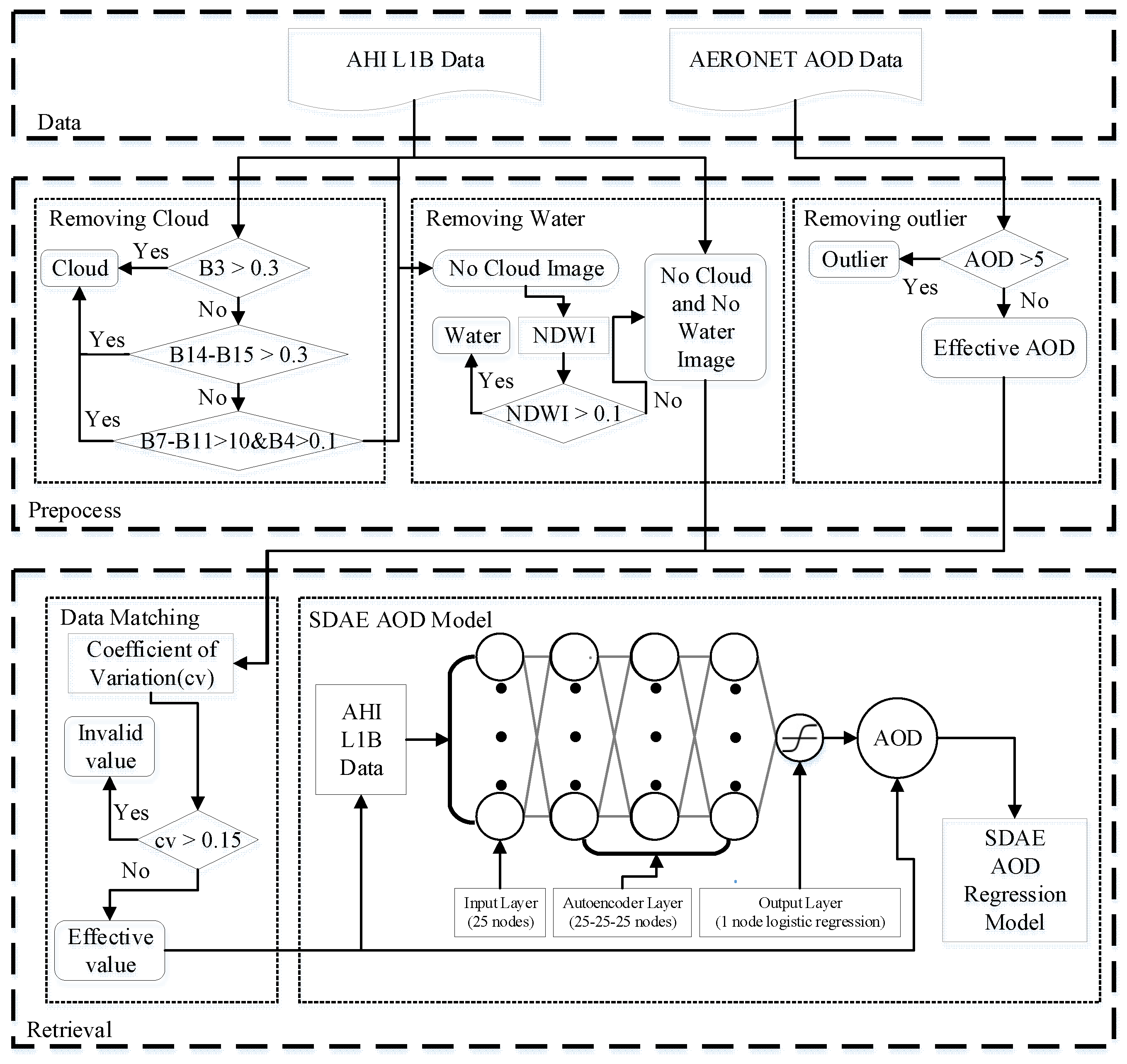
- (1)
- Data preparation: We prepared AHI L1B remote sensing image data taken every ten minutes from 1 January 2016 to 31 December 2016 and AERONET AOD ground observation data in 2016. The AHI L1B data included albedo (reflectance × cos (solar zenith angle (SOZ)) of band 1–band 6), brightness temperature of band 7–band 16, satellite zenith angle, satellite azimuth angle, solar zenith angle, solar azimuth angle, and observation hours (UTC).
- (2)
- Preprocessing: Cloud and water in the remote sensing image data were removed through the cloud removal algorithm and the water removal algorithm. The outlier value judgment method was used to remove the outliers in the AOD ground observation data.
- (3)
- Data matching: We selected the remote sensing image data closest to the observation time of the ground observation data from the preprocessed remote sensing image data. The 3 × 3 remote sensing image grid corresponding to the ground observation data was selected through latitude and longitude, and the coefficient of variation in the grid was used to determine whether the remote sensing image grid met the requirements.
- (4)
- Model establishment: Each band of the 3 × 3 remote sensing image grid was averaged to obtain the training data, which were input into the SDAE model to establish an AOD regression model.
3.1. Prepossessing of the AHI L1B Data
Band 14 − Band 15 < −0.5
Band 7 − Band 11 > 10 and Band 4 > 0.1
3.2. AERONET AOD Outlier Removal
3.3. Data Matching
3.4. SDAE Model
3.5. AHI AOD Model Estimation via the SDAE
4. Results
4.1. Model Evaluation
- (a)
- Correlation Coefficient ():
- (b)
- Mean Relative Error ()
- (c)
- Root Mean Square Error ()
- (d)
- Within .
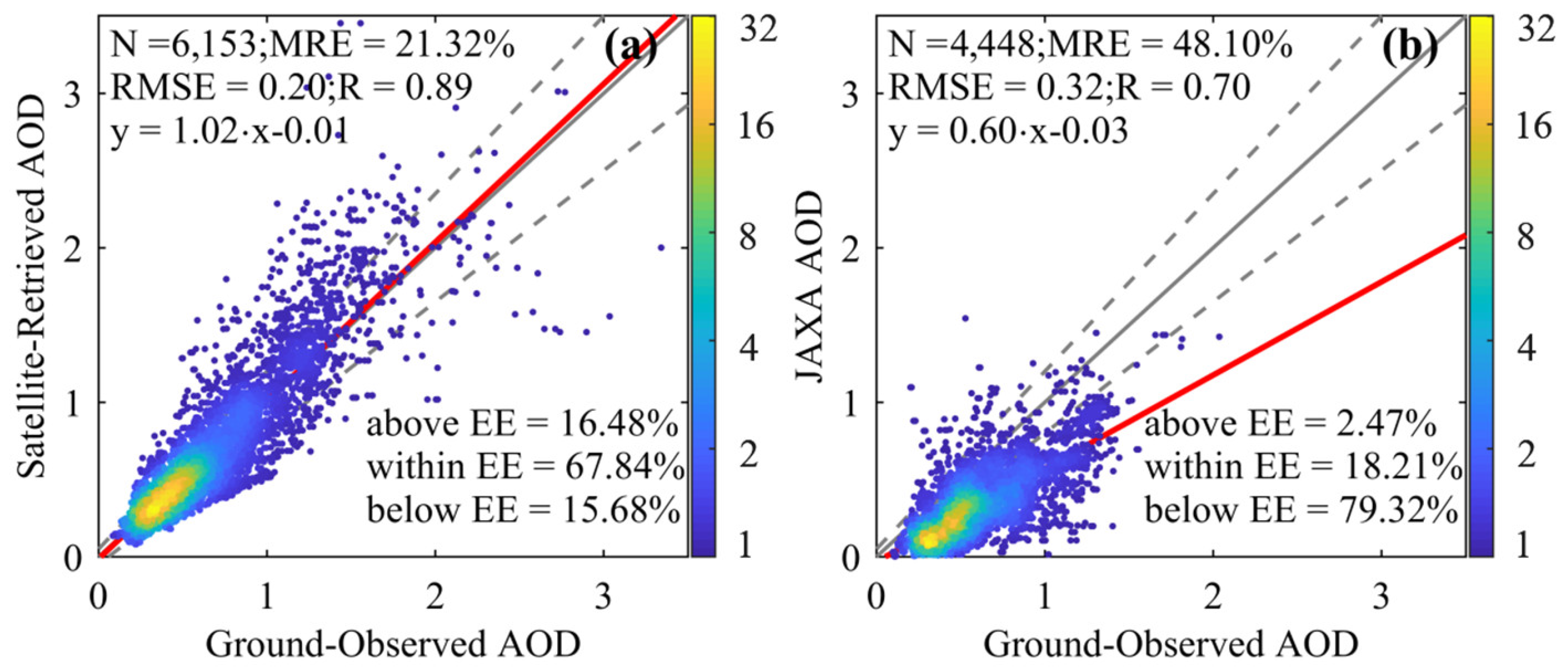
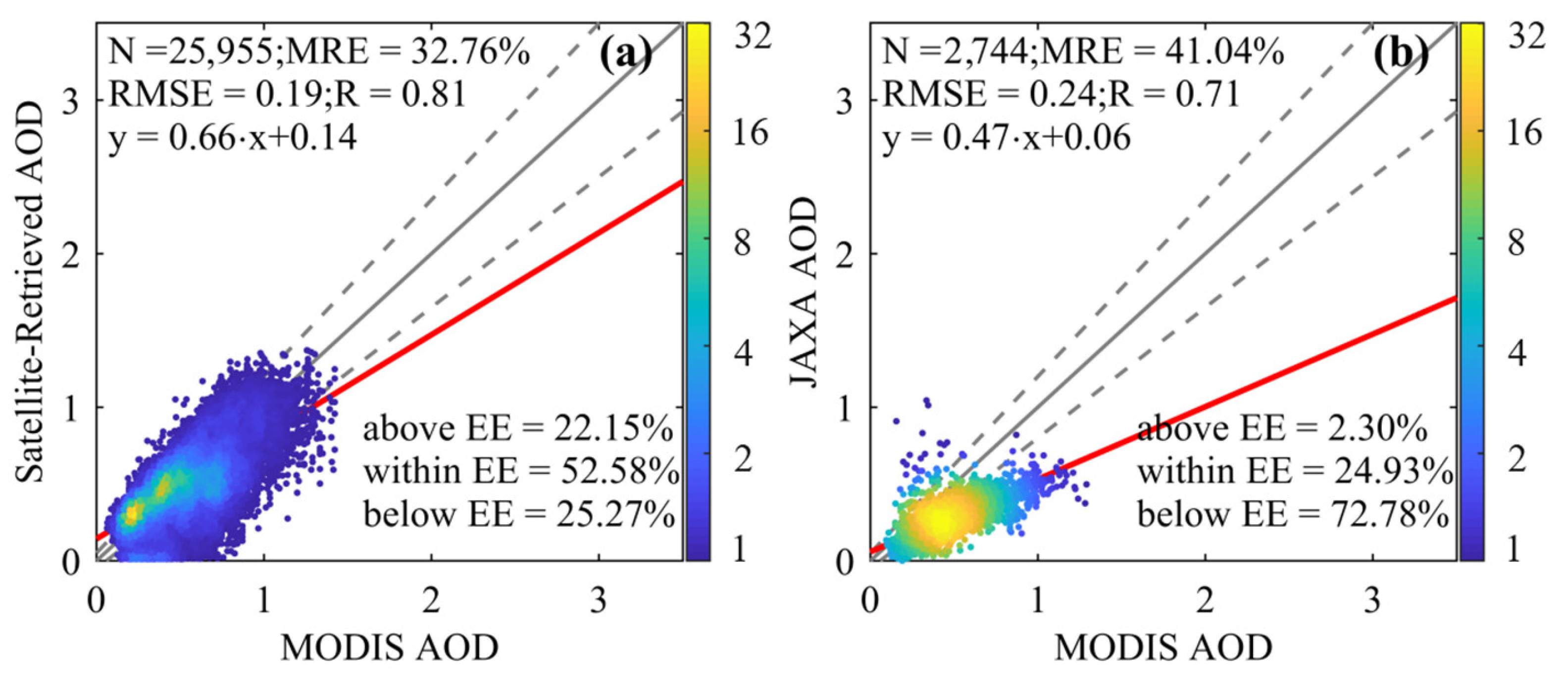
4.2. Validation of the Retrieved AOD
4.2.1. Comparison of JAXA AOD with Ground-Observed AOD
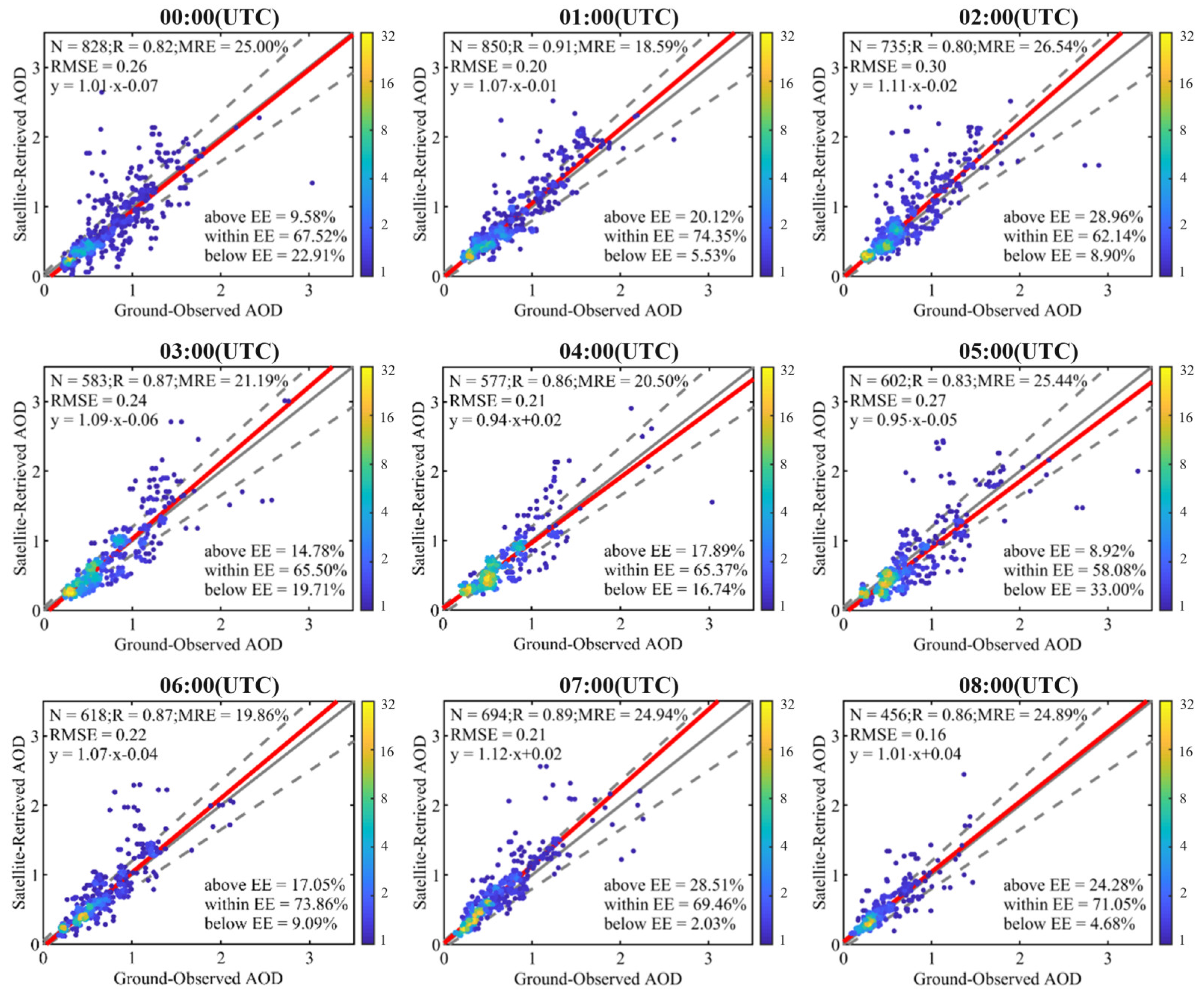
4.2.2. Hourly AOD Validation
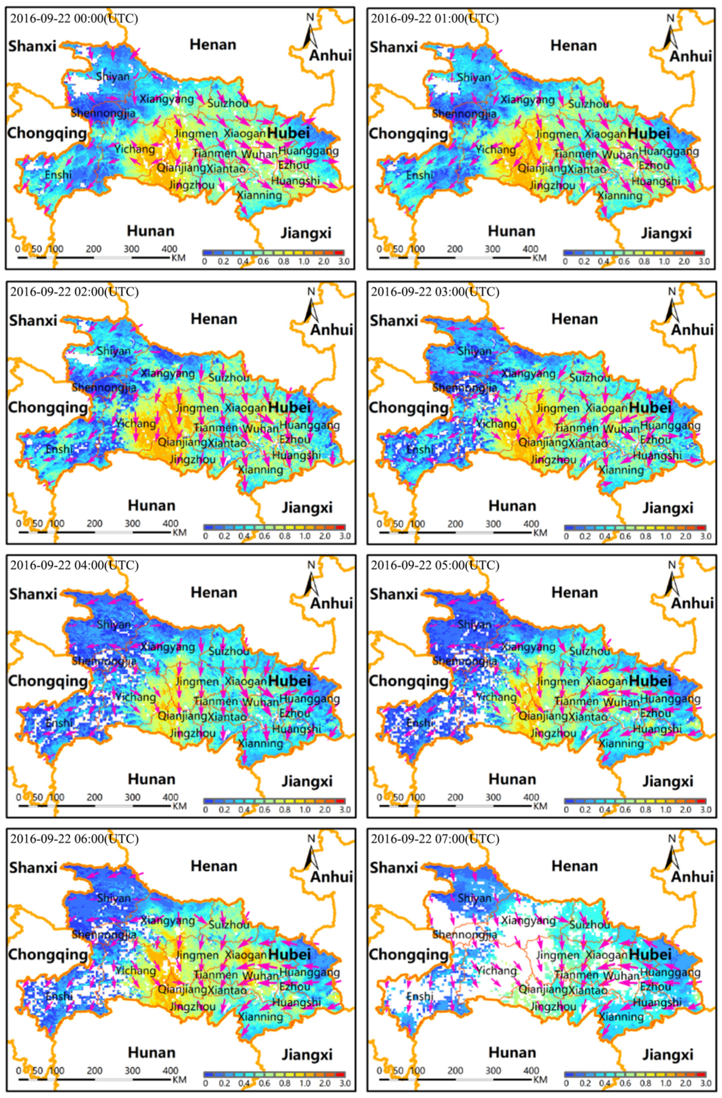
4.3. Hourly Patterns of AOD Distribution
4.4. Discussion
5. Conclusions
Author Contributions
Funding
Data Availability Statement
Conflicts of Interest
Appendix A

| Site | Abbreviation | Site | Abbreviation | Site | Abbreviation |
|---|---|---|---|---|---|
| ‘Alishan’ | ALI | ‘Hankuk_UFS’ | HAN | ‘NGHIA_DO’ | NGH |
| ‘Anmyon’ | ANM | ‘Hokkaido_University’ | HOK | ‘Nong_Khai’ | NON |
| ‘Baengnyeong’ | BAE | ‘Hong_Kong_Sheung’ | HON | ‘Noto’ | NOT |
| ‘Bandung’ | BAN | ‘Irkutsk’ | IRK | ‘Omkoi’ | OMK |
| ‘Beijing_CAMS’ | BCA | ‘Jabiru’ | JAB | ‘Osaka’ | OSA |
| ‘Beijing’ | BJ | ‘KORUS_Baeksa’ | KBK | ‘Palangkaraya’ | PAL |
| ‘Birdsville’ | BS | ‘KORUS_Daegwallyeong’ | KDW | ‘Pontianak’ | PON |
| ‘Canberra’ | CB | ‘KORUS_Iksan’ | KIK | ‘Pusan_NU’ | PUS |
| ‘Chen_Kung_Univ’ | CKU | ‘KORUS_Kyungpook_NU’ | KKN | ‘Seoul_SNU’ | SEO |
| ‘Chiang_Mai_Met_Sta’ | CMM | ‘KORUS_Mokpo_NU’ | KMN | ‘Shirahama’ | SHI |
| ‘Chiayi’ | CHI | ‘KORUS_NIER’ | KNI | ‘Silpakorn_Univ’ | SIL |
| ‘Dalanzadgad’ | DAL | ‘KORUS_Olympic_Park’ | KOP | ‘Singapore’ | SIN |
| ‘Dongsha_Island’ | DON | ‘KORUS_Songchon’ | KSC | ‘Son_La’ | SON |
| ‘Douliu’ | DOU | ‘KORUS_Taehwa’ | KTH | ‘Songkhla_Met_Sta’ | SMS |
| ‘EPA_NCU’ | EPA | ‘KORUS_UNIST_Ulsan’ | KUU | ‘Taipei_CWB’ | TPC |
| ‘Fowlers_Gap’ | FOW | ‘Lake_Argyle’ | LAG | ‘USM_Penang’ | USM |
| ‘Fukuoka’ | FUK | ‘Lake_Lefroy’ | LLF | ‘Ubon_Ratchathani’ | UBO |
| ‘GOT_Seaprism’ | GOT | ‘Luang_Namtha’ | LNT | ‘XiangHe’ | XIA |
| ‘Gandhi_College’ | GAN | ‘Lucinda’ | LCD | ‘Yonsei_University’ | YON |
| ‘Gangneung_WNU’ | GAN | ‘Lulin’ | LUL | ||
| ‘Gosan_SNU’ | GOS | ‘Makassar’ | MAK |
References
- McMurry, P.H. A review of atmospheric aerosol measurements. Atmos. Environ. 2000, 34, 1959–1999. [Google Scholar] [CrossRef]
- Kaufman, Y.J.; Fraser, R.S. Light Extinction by Aerosols during Summer Air Pollution. J. Clim. Appl. Meteorol. 1983, 22, 1694–1706. [Google Scholar] [CrossRef]
- Hsu, N.C.; Si-Chee, T.; King, M.D.; Herman, J.R. Aerosol properties over bright-reflecting source regions. IEEE Trans. Geosci. Remote Sens. 2004, 42, 557–569. [Google Scholar] [CrossRef]
- Pöschl, U. Atmospheric Aerosols: Composition, Transformation, Climate and Health Effects. Angew. Chem. Int. Ed. 2005, 44, 7520–7540. [Google Scholar] [CrossRef]
- Ren, M.; Li, N.; Wang, Z.; Liu, Y.; Chen, X.; Chu, Y.; Li, X.; Zhu, Z.; Tian, L.; Xiang, H. The short-term effects of air pollutants on respiratory disease mortality in Wuhan, China: Comparison of time-series and case-crossover analyses. Sci. Rep. 2017, 7, 40482. [Google Scholar] [CrossRef]
- Kaufman, Y.J. Satellite sensing of aerosol absorption. J. Geophys. Res. Atmos. 1987, 92, 4307–4317. [Google Scholar] [CrossRef]
- Li, X.; Huang, S.; Jiao, A.; Yang, X.; Yun, J.; Wang, Y.; Xue, X.; Chu, Y.; Liu, F.; Liu, Y.; et al. Association between ambient fine particulate matter and preterm birth or term low birth weight: An updated systematic review and meta-analysis. Environ. Pollut. 2017, 227, 596–605. [Google Scholar] [CrossRef]
- Schwartz, S.E.; Andreae, M.O. Uncertainty in Climate Change Caused by Aerosols. Science 1996, 272, 1121. [Google Scholar] [CrossRef]
- Liu, J.; Li, Z. Estimation of cloud condensation nuclei concentration from aerosol optical quantities: Influential factors and uncertainties. Atmos. Chem. Phys. 2014, 14, 471–483. [Google Scholar] [CrossRef]
- Weigum, N.; Schutgens, N.; Stier, P. Effect of aerosol subgrid variability on aerosol optical depth and cloud condensation nuclei: Implications for global aerosol modelling. Atmos. Chem. Phys. 2016, 16, 13619–13639. [Google Scholar] [CrossRef]
- Stier, P.; van den Heever, S.C.; Christensen, M.W.; Gryspeerdt, E.; Dagan, G.; Saleeby, S.M.; Bollasina, M.; Donner, L.; Emanuel, K.; Ekman, A.M.L.; et al. Multifaceted aerosol effects on precipitation. Nat. Geosci. 2024, 17, 719–732. [Google Scholar] [CrossRef]
- Kaufman, Y.J.; Tanré, D.; Remer, L.A.; Vermote, E.F.; Chu, A.; Holben, B.N. Operational remote sensing of tropospheric aerosol over land from EOS moderate resolution imaging spectroradiometer. J. Geophys. Res. Atmos. 1997, 102, 17051–17067. [Google Scholar] [CrossRef]
- Remer, L.A.; Mattoo, S.; Levy, R.C.; Munchak, L.A. MODIS 3 km aerosol product: Algorithm and global perspective. Atmos. Meas. Tech. 2013, 6, 1829–1844. [Google Scholar] [CrossRef]
- Barbosa, P.M.; Grégoire, J.-M.; Pereira, J.M.C. An Algorithm for Extracting Burned Areas from Time Series of AVHRR GAC Data Applied at a Continental Scale. Remote Sens. Environ. 1999, 69, 253–263. [Google Scholar] [CrossRef]
- Holben, B.; Vermote, E.; Kaufman, Y.J.; Tanre, D.; Kalb, V. Aerosol retrieval over land from AVHRR data-application for atmospheric correction. IEEE Trans. Geosci. Remote Sens. 1992, 30, 212–222. [Google Scholar] [CrossRef]
- Liu, G.-R.; Lin, T.-H.; Kuo, T.-H. Estimation of aerosol optical depth by applying the optimal distance number to NOAA AVHRR data. Remote Sens. Environ. 2002, 81, 247–252. [Google Scholar] [CrossRef]
- Hsu, N.C.; Lee, J.; Sayer, A.M.; Carletta, N.; Chen, S.H.; Tucker, C.J.; Holben, B.N.; Tsay, S.C. Retrieving near-global aerosol loading over land and ocean from AVHRR. J. Geophys. Res. Atmos. 2017, 122, 9968–9989. [Google Scholar] [CrossRef]
- Vachon, F. Remote sensing of aerosols over North American land surfaces from POLDER and MODIS measurements. Atmos. Environ. 2004, 38, 3501–3515. [Google Scholar] [CrossRef]
- Koukouli, M.E.; Balis, D.S.; Amiridis, V.; Kazadzis, S.; Bais, A.; Nickovic, S.; Torres, O. Aerosol variability over Thessaloniki using ground based remote sensing observations and the TOMS aerosol index. Atmos. Environ. 2006, 40, 5367–5378. [Google Scholar] [CrossRef]
- Kauppi, A.; Kolmonen, P.; Laine, M.; Tamminen, J. Aerosol-type retrieval and uncertainty quantification from OMI data. Atmos. Meas. Tech. 2017, 10, 4079–4098. [Google Scholar] [CrossRef]
- de Leeuw, G.; Sogacheva, L.; Rodriguez, E.; Kourtidis, K.; Georgoulias, A.K.; Alexandri, G.; Amiridis, V.; Proestakis, E.; Marinou, E.; Xue, Y.; et al. Two decades of satellite observations of AOD over mainland China using ATSR-2, AATSR and MODIS/Terra: Data set evaluation and large-scale patterns. Atmos. Chem. Phys. 2018, 18, 1573–1592. [Google Scholar] [CrossRef]
- Kim, J.; Yoon, J.M.; Ahn, M.H.; Sohn, B.J.; Lim, H.S. Retrieving aerosol optical depth using visible and mid-IR channels from geostationary satellite MTSAT-1R. Int. J. Remote Sens. 2008, 29, 6181–6192. [Google Scholar] [CrossRef]
- Lipponen, A.; Mielonen, T.; Pitkänen, M.R.A.; Levy, R.C.; Sawyer, V.R.; Romakkaniemi, S.; Kolehmainen, V.; Arola, A. Bayesian aerosol retrieval algorithm for MODIS AOD retrieval over land. Atmos. Meas. Tech. 2018, 11, 1529–1547. [Google Scholar] [CrossRef]
- Xiao, Q.; Zhang, H.; Choi, M.; Li, S.; Kondragunta, S.; Kim, J.; Holben, B.; Levy, R.C.; Liu, Y. Evaluation of VIIRS, GOCI, and MODIS Collection 6 AOD retrievals against ground sunphotometer observations over East Asia. Atmos. Chem. Phys. 2016, 16, 1255–1269. [Google Scholar] [CrossRef]
- Benas, N.; Beloconi, A.; Chrysoulakis, N. Estimation of urban PM10 concentration, based on MODIS and MERIS/AATSR synergistic observations. Atmos. Environ. 2013, 79, 448–454. [Google Scholar] [CrossRef]
- Kahn, R.A.; Gaitley, B.J. An analysis of global aerosol type as retrieved by MISR. J. Geophys. Res. Atmos. 2015, 120, 4248–4281. [Google Scholar] [CrossRef]
- Witek, M.L.; Diner, D.J.; Garay, M.J.; Xu, F.; Bull, M.A.; Seidel, F.C. Improving MISR AOD Retrievals With Low-Light-Level Corrections for Veiling Light. IEEE Trans. Geosci. Remote Sens. 2018, 56, 1251–1268. [Google Scholar] [CrossRef]
- Pang, J.; Liu, Z.; Wang, X.; Bresch, J.; Ban, J.; Chen, D.; Kim, J. Assimilating AOD retrievals from GOCI and VIIRS to forecast surface PM2.5 episodes over Eastern China. Atmos. Environ. 2018, 179, 288–304. [Google Scholar] [CrossRef]
- Sun, L.; Sun, C.; Liu, Q.; Zhong, B. Aerosol optical depth retrieval by HJ-1/CCD supported by MODIS surface reflectance data. Sci. China Earth Sci. 2010, 53, 74–80. [Google Scholar] [CrossRef]
- Zhang, M.; Tang, J.; Dong, Q.; Duan, H.; Shen, Q. Atmospheric correction of HJ-1 CCD imagery over turbid lake waters. Opt. Express 2014, 22, 7906. [Google Scholar] [CrossRef]
- Ou, Y.; Chen, F.; Zhao, W.; Yan, X.; Zhang, Q. Landsat 8-based inversion methods for aerosol optical depths in the Beijing area. Atmos. Pollut. Res. 2017, 8, 267–274. [Google Scholar] [CrossRef]
- Zhang, L.; Xu, S.; Wang, L.; Cai, K.; Ge, Q. Retrieval and Validation of Aerosol Optical Depth by using the GF-1 Remote Sensing Data. IOP Conf. Ser. Earth Environ. Sci. 2017, 68, 012001. [Google Scholar] [CrossRef]
- Zhongting, W.; Jinyuan, X.I.N.; Songlin, J.I.A.; Qing, L.I.; Liangfu, C.; Shaohua, Z. Retrieval of AOD from GF-1 16 m camera via DDV algorithm. Natl. Remote Sens. Bull. 2015, 19, 530–538. [Google Scholar] [CrossRef]
- Lu, S.Q.; Chen, W.M.; Gao, Q.X. Using 6S Model to Retrieve Aerosol Optical Depth above Land from GMS5 Satellite Data. Trans Atmos Sci 2006, 29, 669–675. [Google Scholar]
- Ceamanos, X.; Six, B.; Moparthy, S.; Carrer, D.; Georgeot, A.; Gasteiger, J.; Riedi, J.; Attié, J.-L.; Lyapustin, A.; Katsev, I. Instantaneous aerosol and surface retrieval using satellites in geostationary orbit (iAERUS-GEO)—Estimation of 15 min aerosol optical depth from MSG/SEVIRI and evaluation with reference data. Atmos. Meas. Tech. 2023, 16, 2575–2599. [Google Scholar] [CrossRef]
- Mei, L.; Xue, Y.; Wang, Y.; Hou, T.; Guang, J.; Li, Y.; Xu, H.; Wu, C.; He, X.; Dong, J.; et al. Prior information supported aerosol optical depth retrieval using FY2D data. In Proceedings of the 2011 IEEE International Geoscience and Remote Sensing Symposium, Vancouver, BC, Canada, 24–29 July 2011; pp. 2677–2680. [Google Scholar]
- Choi, M.; Kim, J.; Lee, J.; Kim, M.; Park, Y.-J.; Jeong, U.; Kim, W.; Hong, H.; Holben, B.; Eck, T.F.; et al. GOCI Yonsei Aerosol Retrieval (YAER) algorithm and validation during the DRAGON-NE Asia 2012 campaign. Atmos. Meas. Tech. 2016, 9, 1377–1398. [Google Scholar] [CrossRef]
- Jeong, J.I.; Park, R.J. Efficacy of dust aerosol forecasts for East Asia using the adjoint of GEOS-Chem with ground-based observations. Environ. Pollut. 2018, 234, 885–893. [Google Scholar] [CrossRef]
- Prata, A.T.; Grainger, R.G.; Taylor, I.A.; Povey, A.C.; Proud, S.R.; Poulsen, C.A. Uncertainty-bounded estimates of ash cloud properties using the ORAC algorithm: Application to the 2019 Raikoke eruption. Atmos. Meas. Tech. 2022, 15, 5985–6010. [Google Scholar] [CrossRef]
- She, L.; Zhang, H.K.; Li, Z.; de Leeuw, G.; Huang, B. Himawari-8 Aerosol Optical Depth (AOD) Retrieval Using a Deep Neural Network Trained Using AERONET Observations. Remote Sens. 2020, 12, 4125. [Google Scholar] [CrossRef]
- She, L.; Zhang, H.; Wang, W.; Wang, Y.; Shi, Y. Evaluation of the Multi-Angle Implementation of Atmospheric Correction (MAIAC) Aerosol Algorithm for Himawari-8 Data. Remote Sens. 2019, 11, 2771. [Google Scholar] [CrossRef]
- Lyapustin, A.; Wang, Y.; Korkin, S.; Huang, D. MODIS Collection 6 MAIAC algorithm. Atmos. Meas. Tech. 2018, 11, 5741–5765. [Google Scholar] [CrossRef]
- Sayer, A.M.; Hsu, N.C.; Lee, J.; Kim, W.V.; Dubovik, O.; Dutcher, S.T.; Huang, D.; Litvinov, P.; Lyapustin, A.; Tackett, J.L.; et al. Validation of SOAR VIIRS Over-Water Aerosol Retrievals and Context Within the Global Satellite Aerosol Data Record. J. Geophys. Res. Atmos. 2018, 123, 13496–13526. [Google Scholar] [CrossRef]
- Wang, L.; Gong, W.; Xia, X.; Zhu, J.; Li, J.; Zhu, Z. Long-term observations of aerosol optical properties at Wuhan, an urban site in Central China. Atmos. Environ. 2015, 101, 94–102. [Google Scholar] [CrossRef]
- Bai, T.; Wang, L.; Yin, D.; Sun, K.; Chen, Y.; Li, W.; Li, D. Deep learning for change detection in remote sensing: A review. Geo-Spat. Inf. Sci. 2023, 26, 262–288. [Google Scholar] [CrossRef]
- Bai, T.; An, Q.; Deng, S.; Li, P.; Chen, Y.; Sun, K.; Zheng, H.; Song, Z. A Novel UNet 3+ Change Detection Method Considering Scale Uncertainty in High-Resolution Imagery. Remote Sens. 2024, 16, 1846. [Google Scholar] [CrossRef]
- Vincent, P.; Larochelle, H.; Lajoie, I.; Bengio, Y.; Manzagol, P.-A.; Bottou, L. Stacked denoising autoencoders: Learning useful representations in a deep network with a local denoising criterion. J. Mach. Learn. Res. 2010, 11, 3371–3408. [Google Scholar]
- Li, W.; Fu, H.; Yu, L.; Gong, P.; Feng, D.; Li, C.; Clinton, N. Stacked Autoencoder-based deep learning for remote-sensing image classification: A case study of African land-cover mapping. Int. J. Remote Sens. 2016, 37, 5632–5646. [Google Scholar] [CrossRef]
- She, L.; Xue, Y.; Yang, X.; Guang, J.; Li, Y.; Che, Y.; Fan, C.; Xie, Y. Dust Detection and Intensity Estimation Using Himawari-8/AHI Observation. Remote Sens. 2018, 10, 490. [Google Scholar] [CrossRef]


| Site | Number | Longitude | Latitude | Elevation (m) | AOD (Means and Standard Deviations) | Site | Number | Longitude | Latitude | Elevation (m) | AOD (Means and Standard Deviations) |
|---|---|---|---|---|---|---|---|---|---|---|---|
| ALI | 20 | 120.81 | 23.51 | 2216 | 0.34 ± 0.20 | KNI | 181 | 126.64 | 37.57 | 25 | 0.40 ± 0.23 |
| ANM | 871 | 126.33 | 36.54 | 1450 | 0.32 ± 0.28 | KOP | 64 | 127.12 | 37.52 | 180 | 0.51 ± 0.30 |
| BAE | 202 | 124.63 | 37.97 | 380 | 0.27 ± 0.20 | KSC | 95 | 127.49 | 37.34 | 75 | 0.51 ± 0.38 |
| BAN | 95 | 107.61 | −6.89 | 3 | 0.32 ± 0.15 | KTH | 83 | 127.31 | 37.31 | 65 | 0.41 ± 0.23 |
| BCA | 967 | 116.32 | 39.93 | 43 | 0.40 ± 0.40 | KUU | 268 | 129.19 | 35.58 | 3 | 0.36 ± 0.17 |
| BJ | 606 | 116.38 | 39.98 | 52 | 0.37 ± 0.35 | LAG | 1470 | 128.75 | −16.11 | 1880 | 0.08 ± 0.07 |
| BS | 1540 | 139.35 | −25.90 | 3 | 0.05 ± 0.03 | LLF | 295 | 121.71 | −31.26 | 3 | 0.07 ± 0.03 |
| CB | 765 | 149.11 | −35.27 | 560 | 0.05 ± 0.03 | LNT | 179 | 101.42 | 20.93 | 1030 | 0.43 ± 0.33 |
| CKU | 113 | 120.22 | 23.00 | 780 | 0.55 ± 0.39 | LCD | 555 | 146.39 | −18.52 | 3 | 0.10 ± 0.04 |
| CMM | 597 | 98.97 | 18.77 | 1210 | 0.44 ± 0.30 | LUL | 27 | 120.87 | 23.47 | 1950 | 0.06 ± 0.07 |
| CHI | 298 | 120.50 | 23.50 | 230 | 0.61 ± 0.30 | MAK | 317 | 119.57 | −5.00 | 3 | 0.23 ± 0.16 |
| DAL | 209 | 104.42 | 43.58 | 1040 | 0.08 ± 0.06 | NGH | 88 | 105.80 | 21.05 | 210 | 0.64 ± 0.29 |
| DON | 24 | 116.73 | 20.70 | 15 | 0.26 ± 0.23 | NON | 81 | 102.72 | 17.88 | 1560 | 0.60 ± 0.41 |
| DOU | 87 | 120.55 | 23.71 | 1650 | 0.63 ± 0.32 | NOT | 95 | 137.14 | 37.33 | 2800 | 0.21 ± 0.17 |
| EPA | 272 | 121.19 | 24.97 | 360 | 0.27 ± 0.17 | OMK | 610 | 98.43 | 17.80 | 1230 | 0.23 ± 0.17 |
| FOW | 1993 | 141.70 | −31.09 | 3 | 0.04 ± 0.03 | OSA | 228 | 135.59 | 34.65 | 22 | 0.25 ± 0.21 |
| FUK | 202 | 130.48 | 33.52 | 12 | 0.32 ± 0.20 | PAL | 44 | 113.95 | −2.23 | 3 | 0.45 ± 0.36 |
| GOT | 82 | 101.41 | 9.29 | 1890 | 0.24 ± 0.28 | PON | 30 | 109.19 | 0.08 | 3 | 0.90 ± 0.93 |
| GAN | 771 | 84.13 | 25.87 | 5200 | 0.83 ± 0.47 | PUS | 1053 | 129.08 | 35.24 | 35 | 0.23 ± 0.20 |
| GAN | 1374 | 128.87 | 37.77 | 220 | 0.20 ± 0.16 | SEO | 495 | 126.95 | 37.46 | 42 | 0.35 ± 0.29 |
| GOS | 228 | 126.16 | 33.29 | 3 | 0.28 ± 0.17 | SHI | 566 | 135.36 | 33.69 | 18 | 0.18 ± 0.14 |
| HAN | 721 | 127.27 | 37.34 | 38 | 0.31 ± 0.27 | SIL | 964 | 100.04 | 13.82 | 5 | 0.48 ± 0.21 |
| HOK | 264 | 141.34 | 43.08 | 30 | 0.23 ± 0.21 | SIN | 52 | 103.78 | 1.30 | 15 | 0.55 ± 0.38 |
| HON | 37 | 114.12 | 22.48 | 8 | 0.37 ± 0.21 | SON | 91 | 103.91 | 21.33 | 1120 | 0.78 ± 0.55 |
| IRK | 94 | 103.09 | 51.80 | 430 | 0.24 ± 0.22 | SMS | 54 | 100.61 | 7.18 | 80 | 0.31 ± 0.23 |
| JAB | 726 | 132.89 | −12.66 | 3 | 0.13 ± 0.08 | TPC | 123 | 121.50 | 25.03 | 9 | 0.35 ± 0.21 |
| KBK | 75 | 127.57 | 37.41 | 90 | 0.45 ± 0.33 | USM | 287 | 100.30 | 5.36 | 3 | 0.35 ± 0.31 |
| KDW | 25 | 128.76 | 37.69 | 320 | 0.35 ± 0.16 | UBO | 283 | 104.87 | 15.25 | 170 | 0.31 ± 0.31 |
| KIK | 222 | 127.01 | 35.96 | 680 | 0.48 ± 0.23 | XIA | 874 | 116.96 | 39.75 | 40 | 0.38 ± 0.39 |
| KKN | 217 | 128.61 | 35.89 | 410 | 0.43 ± 0.20 | YON | 881 | 126.94 | 37.56 | 28 | 0.33 ± 0.26 |
| KMN | 289 | 126.44 | 34.91 | 15 | 0.31 ± 0.17 |
| Site | Number of Data | Mean | Median | Std | Min | Max | Time Range (Year) |
|---|---|---|---|---|---|---|---|
| ALL AERONET | 24,413 | 0.2703 | 0.1547 | 0.2989 | 0.0094 | 3.0357 | 2015–2017 |
| Wuhan University Site | 6945 | 0.6273 | 0.5250 | 0.3629 | 0.0850 | 2.9396 | 2016 |
| Method | R | MRE | RMSE | Within EE |
|---|---|---|---|---|
| ELM | 0.74 | 104% | 0.21 | 43% |
| BPNN | 0.87 | 76% | 0.18 | 52% |
| SVM | 0.91 | 49% | 0.14 | 79% |
| GRNN | 0.94 | 36% | 0.09 | 85% |
| SDAE | 0.98 | 26% | 0.06 | 92% |
Disclaimer/Publisher’s Note: The statements, opinions and data contained in all publications are solely those of the individual author(s) and contributor(s) and not of MDPI and/or the editor(s). MDPI and/or the editor(s) disclaim responsibility for any injury to people or property resulting from any ideas, methods, instructions or products referred to in the content. |
© 2025 by the authors. Licensee MDPI, Basel, Switzerland. This article is an open access article distributed under the terms and conditions of the Creative Commons Attribution (CC BY) license (https://creativecommons.org/licenses/by/4.0/).
Share and Cite
Deng, S.; Bai, T.; Chen, Z.; Chen, Y. A Novel Aerosol Optical Depth Retrieval Method Based on SDAE from Himawari-8/AHI Next-Generation Geostationary Satellite in Hubei Province. Remote Sens. 2025, 17, 1396. https://doi.org/10.3390/rs17081396
Deng S, Bai T, Chen Z, Chen Y. A Novel Aerosol Optical Depth Retrieval Method Based on SDAE from Himawari-8/AHI Next-Generation Geostationary Satellite in Hubei Province. Remote Sensing. 2025; 17(8):1396. https://doi.org/10.3390/rs17081396
Chicago/Turabian StyleDeng, Shiquan, Ting Bai, Zhe Chen, and Yepei Chen. 2025. "A Novel Aerosol Optical Depth Retrieval Method Based on SDAE from Himawari-8/AHI Next-Generation Geostationary Satellite in Hubei Province" Remote Sensing 17, no. 8: 1396. https://doi.org/10.3390/rs17081396
APA StyleDeng, S., Bai, T., Chen, Z., & Chen, Y. (2025). A Novel Aerosol Optical Depth Retrieval Method Based on SDAE from Himawari-8/AHI Next-Generation Geostationary Satellite in Hubei Province. Remote Sensing, 17(8), 1396. https://doi.org/10.3390/rs17081396