Hyperspectral Image Reconstruction Based on Blur–Kernel–Prior and Spatial–Spectral Attention

Abstract

Given the problem of spatial detail loss and spectral feature degradation in hyperspectral images (HSIs) characterized as blur, often caused by noise during image acquisition, and methods of removing blur noise designed on HSIs being insufficient, we propose an HSI reconstruction network based on a Blur–Kernel–Prior (BKP) method and Spectral–Spatial Attention (SSA) strategy for noise removal and reconstruction of HSIs. Specifically, a grouping strategy is designed to segment the HSIs into spectral dimension sub-images, and the BKP module, based on U-Net, learns the spatially adaptive blur kernel to extract and remove blurred features from each sub-image while preserving spatial features with spatial resolution. Subsequently, the SSA block is employed to extract shallow features, details, and edge information using a hybrid 2D–3D convolution from the sub-images, followed by deep feature extraction using a deep ResNet and multi-head attention (MSA) on the merged image to maximize the preservation of spectral dimension information. The $L_1$ loss function, combined with spectral dimension loss and peak signal-to-noise ratio loss, is utilized to constrain and ensure reconstruction accuracy. Experiments on both synthetic and real datasets demonstrate that our method exhibits excellent performance in reconstructing HSIs affected by blurred noise, outperforming existing methods in terms of quantitative quality and recovery of spectral dimension information.

1. Introduction

Unlike RGB and multispectral images (MSIs), hyperspectral images (HSIs) provide more spectral bands and rich spectral information, revealing detailed intrinsic properties of real-world objects and subtle differences that are often difficult to detect in RGB and MSIs. As a result, HSIs are extensively utilized in various domains, including computer vision and remote sensing, with applications in classification [1,2,3], medical diagnosis [4], detection [5,6], and geological exploration [7]. It is essential that the degradation characterized as blur caused by external and internal noise simultaneously affects the spatial and spectral dimensions of HSIs. In particular, during the acquisition process, factors such as platform vibration [8], scanning errors [9], atmospheric turbulence [10], and sensor electronic noise [11] can lead to the loss of spatial details and the smoothing of spectral features, further impacting related applications. Therefore, the removal of blur noise and the reconstruction that enhances spatial resolution are critical preprocessing steps necessary to improve the quality of HSIs and augment their practical utility [12,13,14].

Unlike machine-learning using a low-rank matrix, tensor representations [2,15] and Singular Value Decomposition (SVD) [16] which result in prolonged processing times and often yields unstable outcomes that are highly sensitive to the configuration of regularization parameters [17,18], deep-learning breakthroughs have revolutionized HIS reconstruction on deblurring through data-driven feature learning [19]. One of the early contributions in this domain is the SSF–CNN method [20], which employs convolution neural networks (CNNs) combined with techniques such as residual learning, dilated convolution, and multi-channel filtering to effectively denoise HSI data. Similarly, a 3D-CNN method [21] was proposed, which integrates 2D CNNs for spectral feature extraction and 3D CNNs with larger convolution kernels to expand the receptive field. The objective of this network is to remove noise by learning cross-band spectral features of HSIs, thereby addressing image degradation. However, while this design allows the trained network to generalize to new images with different spectral bands, it does not fully utilize all spectral bands during the denoising process. Building on these foundations, various reconstructions on deblur algorithms based on 2D CNNs or 3D CNNs have been proposed [22,23,24,25]. For instance, Nonlocal-CNN [24] groups nonlocal similar patches by leveraging the high spectral correlation of HSIs data, using subspace representations where the corresponding representation coefficients are termed eigenimages. Hou et al. [25] introduced a cooperative self-supervised CNN combined with non-convex regularization, which enhances the local smoothness of extracted features while preserving sharp edges. Despite their effectiveness, CNNs often overemphasize local contextual information while neglecting long-range dependencies within the data. Additionally, CNN-based methods that limit receptive field (<15 × 15 pixels) compromised long-range dependency modeling typically incur >15% mutual information loss across spectral bands due to localized feature extraction mechanisms [25,26].

The attention mechanism, initially introduced for sequential data analysis in natural language processing (NLP), has shown great potential in addressing the limitations of CNNs [27,28]. Unlike CNNs, the attention mechanism excels in capturing global information by focusing on relevant features while processing data sequentially and has been applied successfully for RGB image denoising and reconstruction [29]. However, when applied to high-dimensional data such as HSIs, the attention mechanism may encounter challenges due to the large number of parameters in the network. This can result in slow training processes and reduced effectiveness in tasks like HSI denoising and reconstruction. To overcome these challenges, researchers have explored various strategies. One approach involves applying downsampling methods to HSIs with blurred noise, which helps reduce the number of parameters through CNN layers while still effectively capturing global features [26]. Another strategy focuses on the correlation between spectral bands, employing a band-attention mechanism to lower training costs while preserving essential spectral information [30,31,32]. These advancements demonstrate how optimized attention mechanisms can strike a balance between computational efficiency and performance, making them a promising solution for HSI denoising and reconstruction tasks.

One of the significant challenges in HSI reconstruction on deblur is the presence of various types of noise introduced by imaging sensors and acquisition conditions. Most deep-learning algorithms typically limit their degradation models to address only resolution degradation of input images due to inherent defects in the sensor and optical system, so that relative research often uses bicubic interpolation for downsampling [19,20,33]. However, real-world HSI degradation involves not only resolution loss but also blurring introduced during acquisition. These issues arise from factors such as scanning errors, atmospheric turbulence, and electronic noise, manifesting as a mixture of multiple blurring noises, including motion blur and Gaussian blur. Currently, there is no deep-learning-based reconstruction on the deblur method specifically targeting the challenges posed by low spatial resolution HSIs contaminated by such noise. Recent studies have shown that as image data passes through deep neural networks, the original noise may be amplified [17,34]. This can lead the network to extract features from noisy textures, resulting in inaccurate outcomes. Therefore, our research focuses on mitigating noise in HSIs, which is expected to improve the accuracy of subsequent feature recognition and ground object classification.

To tackle the issues previously mentioned, this paper introduces an HSI reconstruction network grounded in spatial prior denoising, which is designated as BKPSSAnet. The primary contributions of this paper are outlined as follows:

• We present a novel HSI reconstruction method that leverages a Blur–Kernel–Prior neural network for the denoising and reconstruction of HSIs affected by mixed blur noise, marking the first application of this technique in the field.
• The architecture incorporates two distinct modules: a Blur–Kernel–Prior denoising module-based U-Net backbone and a spatial attention feature-reconstruction module. The module implements an end-to-end encoding-decoding process utilizing a dual U-Net architecture, which effectively isolates the blur kernel from the original image. Meanwhile, the spatial attention feature-reconstruction module employs hybrid 2D–3D convolution provided shallow feature extraction locally and attention mechanisms with multi-head attention to facilitate comprehensive deep feature extraction across both spatial and spectral dimensions globally.
• Experimental evaluations conducted on the Cave, Chikusei, and Pavia University datasets, which include mixed simulated noise, demonstrate that our research surpasses the state-of-the-art of deep-learning-based approaches across different image-quality metrics.

2. Related Work

In this section, a review of the algorithms is provided for deblurring noise and image reconstruction in HSIs.

2.1. Traditional Image Blind Deconvolution Model

The classical approach to addressing the blind deconvolution problem in blurry images adopts a joint optimization framework in which both the blur kernel and the latent image are updated with iteration to minimize a loss function that integrates prior knowledge of the kernel and the image. For cases involving high noise levels, a combination of $L_1$ regularization and TV priors is employed to effectively suppress noise and preserve structural details [35,36]. This joint optimization framework proves advantageous in mitigating degenerate solutions, such as the trivial case where $({\mathrm{x}}^{*},{\mathrm{h}}^{*})=(\mathrm{y},\mathrm{I})$, with $\mathrm{I}$ representing the identity operator. Moreover, some approaches explicitly model the blur kernel by considering the camera’s motion trajectory, leveraging optimization techniques or supervised-learning methods to recover both the trajectory and the underlying clean image.

In the HSI acquisition process, external environmental factors tend to be more complex and challenging to manage. In the practically significant non-blind deconvolution tasks, where the blur kernel is presumed to be known, the Poisson deconvolution problem has been a focus of study for several decades, beginning with the foundational Richardson-Lucy algorithm. Contemporary methods have evolved to include advanced techniques such as Plug-and-Play (PnP) frameworks and optimization strategies grounded in Maximum A Posteriori (MAP) estimation [37]. These modern approaches offer enhanced performance and robustness in dealing with the intricacies of deconvolution in HSI data.

There is a method for estimating spatially varying kernels from a single image, which aims to address challenges posed by non-uniform motion blur. Early attempts at estimating these kernels were primarily focused on scenarios involving camera self-motion, under the assumption that the scene was planar and could be mapped to the image plane via a homography. To tackle spatially varying blur resulting from depth differences and moving objects, a strategy was developed to segment the image into a limited number of layers at fixed depths. However, this piece-wise constant model has the drawback of being highly sensitive to how the blurred image is segmented. Another approach, more closely aligned with recent methods, addresses both depth variation within the scene and the presence of moving objects by incorporating local predictions of motion blur. This approach utilizes a set of predefined linear motion kernels parameterized by their length and direction. CNNs are employed to predict the probability distribution of these kernel parameters at the patch level. Subsequently, a Markov Random Field (MRF) is used to enforce motion smoothness, transforming patch-level distributions into a dense motion field [18]. For a given blurred image, a Fully Convolution Network (FCN) can directly estimate the dense linear motion field, parameterized by its horizontal and vertical components. To train the FCN, simulated motion fields are used to create synthetic pairs of blurred images and corresponding motion fields. Both of these methods advocate for using a non-blind deblurring approach with the estimated kernels to restore the image, combining an $L_2$ data fitting term with an Expected Patch Log Likelihood (EPLL) image prior [38]. These advanced techniques enhance the capability to effectively manage complex blurring scenarios in single images.

2.2. Effective Estimation of Blur Kernels Based on Deep Learning

In recent years, kernel prediction networks (KPNs) have demonstrated significant potential in various low-level visual tasks, such as burst denoising, optical flow estimation, frame interpolation, stereo matching, and video prediction [39]. KPNs have been particularly effective in the context of burst denoising, where multiple noisy images from the same scene are used to achieve a cleaner output. Cai et al. [40] utilized KPNs to generate denoised estimates for each pixel by computing a weighted average of locally noisy pixels across all input frames in a burst. The weights, or kernels, for this averaging process, are predicted directly from the noisy input bursts using CNNs. This approach enables adaptive and content-aware processing, ensuring the denoising operation is tailored to the local image structure. To further enhance computational efficiency, Xia et al. [41] proposed a basis prediction network. Instead of predicting unique kernels for each pixel, this method predicts a set of global basis kernels shared across the image. Alongside these global kernels, the network predicts pixel-specific mixing coefficients that determine how the global kernels are combined for each pixel in the input burst. This strategy significantly reduces computational complexity while maintaining high-quality denoising performance, making it well-suited for resource-constrained applications. These advancements in kernel prediction networks have paved the way for more efficient and effective solutions to complex denoising and other low-level vision tasks, particularly in scenarios where burst imaging or multi-frame data are available.

In this paper, a dense non-uniform motion-blurred estimation method based on a low-rank representation of the pixel-direction blurred kernel function is used. As in, the per-pixel kernel is modeled as a linear combination of basic elements, but instead of having a single pre-computed basis of elements, Blur–Kernel–Prior (BKP) based on KPN is used to infer a non-parametric basis specific to each input image. In addition, rather than learning kernels to solve the image recovery problem, we research them to fit forward-degenerate models, thus enabling us to utilize existing techniques to solve the inverse problem.

2.3. Attention Mechanisms for HSIs Reconstruction

Originally introduced in the field of natural language processing, the attention mechanism has demonstrated a remarkable capability to manage nonlocal similarities and has since achieved significant success in various computer vision tasks [3,6]. Considering the unique characteristics of HSIs, which possess richer spectral resolution and intricate spatial–spectral relationships compared to RGB images, most existing transformer-based methods incorporate dual constraints on both spatial and spectral information. In the context of HSI reconstruction, attention mechanisms have been employed to enhance the extraction and utilization of spatial–spectral features. Researchers have investigated the integration of transformers with 3D convolutions to facilitate the learning of these features. For instance, Liu et al. proposed a network named Interformer, which incorporates Transformer modules alongside 3D convolutions to capture complex spatial–spectral interactions [42]. Similarly, Hu et al. developed a multi-stage progressive network (MPNet) that utilizes learning and nonlocal channel attention to refine feature details [43].

Despite the innovative nature of these methods, they often encounter challenges due to the quadratic computational complexity intrinsic to attention mechanisms. This perplexity limits the efficiency and scalability of the models, as they predominantly emphasize long-range dependencies within the spectral dimension, potentially underutilizing both global and local spatial information. To address these challenges, a spatial–spectral attention (SSA) model has been proposed. The SSA model is designed to effectively extract and integrate both spatial and spectral information by leveraging local-global spatial–spectral relationships. This approach aims to enhance the performance of HSI reconstruction tasks by balancing computational efficiency with the comprehensive utilization of spatial–spectral features, thereby overcoming the limitations of existing methods.

3. Methodology

In this section, the problem formulation of HSIs denoising the research is first illustrated. Then, the proposed HISR method BKPSSA is described in detail, including four parts: general framework-based group strategy, BKP, SSA, and loss function.

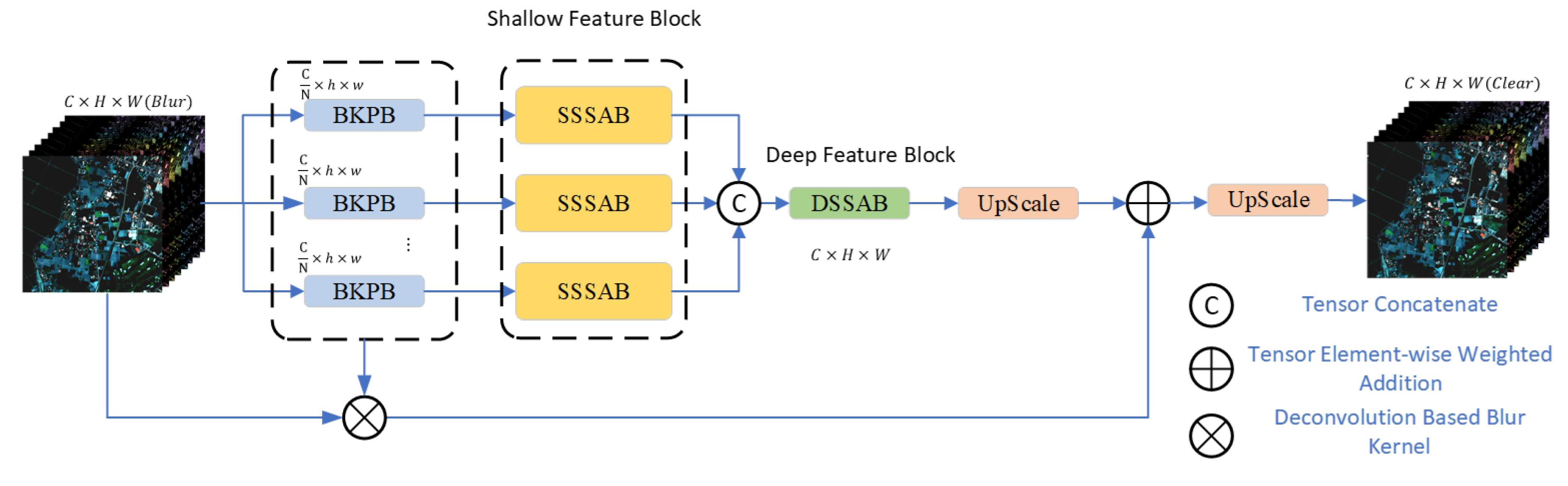
3.1. Overall Architecture

The overall structure of the proposed BKPSSA frame for HIS denoising is illustrated in Figure 1. The BKPSSA HSIs denoising network proposed in this study is based on a group strategy, which will result in a model with fewer parameters, thereby facilitating a more efficient convergence during the training process than traditional CNNs and Attentions [31,44]. The feature extractor and reconstructor use innovative components that simultaneously capture both local and global spatial–spectral interactions. The first part, the BKP module, is designed to learn the blurred kernel and the spatial dimensional relationships of the HSIs. By leveraging U-Net’s symmetric architecture, the BKP module efficiently captures the blur kernel’s prior knowledge and helps restore the spatial consistency of the image. This structure enables the network to focus on the essential spatial–spectral features by preserving key spatial information while mitigating the effects of noise and blur. The second part, the SSA module, is responsible for learning the locally and globally diverse spatial–spectral interactions. The SSA architecture, which combines a hybrid 2D-3D convolutional network with an attention mechanism, can capture both short-range spatial correlations and long-range spectral dependencies. The integration of these two components within the BKPSSA framework not only improves the efficiency of the model but also contributes to its robustness in handling complex degradation issues, making it a powerful approach for HSI reconstruction on denoise tasks. It is essential to emphasize that, unlike conventional denoising models that focus on the removal of Gaussian noise and strip noise, as well as super-resolution tasks that aim to enhance sensor resolution limits, our task concentrates on addressing imaging blur noise caused by external factors, such as Gaussian blur and motion blur, during the acquisition process of hyperspectral camera.

Rather than being limited to conventional Gaussian noise models that consider only additive noise, the degradation of HSIs, whether in the form of blurring or resolution reduction, is often caused by convolution with a blur kernel.

It is agreed that the real HSIs are $I_{HR}\in {\mathbb{R}}^{C\times H\times W}$, and the blurred HSIs are $I_B\in {\mathbb{R}}^{C\times H\times W}$, the spatial and spectral resolution of the blurred HSIs are unchanged compared to the real HSIs, but the signal-to-noise ratio is lower. The relationship between the blurred HSIs $I_B$ and the real HSIs $I_{HR}$ is showing as Equation (1),

$$I_B=K\odot I_{HR}+N$$

(1)

where K is the blurred kernel, the essence of image degradation is the convolution operation of the image with the blurred kernel, shown by the symbol ⊙. N indicates that the blurred image is affected by other linear noises, such as the pretzel noise, Gaussian noise, and so on. Therefore, the recovery reconstruction of blurred HSIs can be regarded as the inverse problem of the degradation process. To establish the model $M_{Rebuild}$, the reconstructed HSIs $I_R$ minimizes the information difference in spatial and spectral dimensions between the reconstructed image $I_{HR}$ and the original image $I_{HR}$. The acquisition of $I_R$ belongs to the following Equation (2),

$$I_R=M_{Rebuild}\left(I_B\right)$$

(2)

To fully utilize the strong correlation between adjacent bands and improve efficiency, many methods based on grouping strategies have been proposed and shown to be superior to other methods. On this basis, the input $I_B$ HSIs are first grouped into G groups according to the spectral channel mode, $I_B=[I_B^1,\cdots ,I_B^g,\cdots ,I_B^G]$.

In this model, the blurred image $I_B$ first undergoes the BKP process. For the local information $I_B^g$, a U-net-based blurred kernel estimation is designed to extract the blurred kernel features $K_g\in {\mathbb{R}}^{{\displaystyle \frac{C}{G}}\times H\times W}$ and the equivalent degraded hyperspectral sub-images $I_{LR}^g\in {\mathbb{R}}^{{\displaystyle \frac{C}{G}}\times s\times s}$ and the equivalent degenerate hyperspectral sub-image $I_{LR}^g\in {\mathbb{R}}^{{\displaystyle \frac{C}{G}}\times h\times w}$ to the following Equation (3),

$$K_g,I_{LR}^g=M_{BKP}\left(I_B^g\right)$$

(3)

The dimension size of $K_g$ depends on the initially given hyperparameters. The spatial-temporal dimensional degradation blurred kernel estimate K for the whole HSIs can be finally obtained after inter-spectral cascading, with the following Equation (4):

$$K=cat(K_1,K_2,\cdots ,K_G))$$

(4)

As for the equivalent degraded hyperspectral sub-image $I_{LR}^g$, it already contains prior degradation information, so it needs to be reconstructed in the spatial–spectral dimension in the SSA structure. In order to finely control the reconstruction, as well as to ensure that the reconstruction accuracy is improved, the sub-images are first reconstructed within the corresponding channel of each sub-image to obtain the SSA reconstructed sub-images $I_R^g\in {\mathbb{R}}^{{\displaystyle \frac{C}{G}}\times H^{\prime }\times w^{\prime }}$, a process known as the Shallow Feature Extraction Block (SFEB), including hybrid 2D-3D convolution which combines 2DCNN utilized at spatial dimension and 3DCNN utilized at spectral dimension. Then cascade each sub-map to obtain the cascade reconstruction image in spectral dimension $I_R^{\prime }{\in \mathbb{R}}^{C\times H^{\prime }\times w^{\prime }}$ to the following Equation (5),

$$I_R^{\prime }=cat(I_R^1,I_R^2,\cdots ,I_R^G)$$

(5)

Obviously, $I_R^{\prime }$ is only a simple cascade of channels, and thus, the error with the original image is still not small, and the spatial dimension is lower than the original image, so it is necessary to carry out reconstruction of the cascade reconstructed image $I_R^{\prime }$, to establish a deep feature extraction module Deep Feature Extraction Block (DFEB) that unlike SFEB can extract spatial–spectral features from the full spectrum, restoring texture detail information in the spatial dimension and spectral characteristics in the spectral dimension, thereby correcting the global spectral loss.

$$I_{deconv}=deconv\left(I_B,K\right)I_R=Up(I_{deconv}+Up\left({I^{\prime }}_R\right))$$

(6)

Finally, in order to reduce the difficulty of training the network and to focus on the high-frequency information, the blurred kernel is deconvoluted with the input blurred image by a filter function $I_{deconv}$ is added directly to the tail of the network. The 1 × 1 convolution after the double-third time is used to adjust the spatial size of the addition operation. Moreover, 1 × 1 convolution after summation is performed to make its spatial size consistent with the original high-resolution HSIs. The above upsampling processes can be represented as Equation (6).

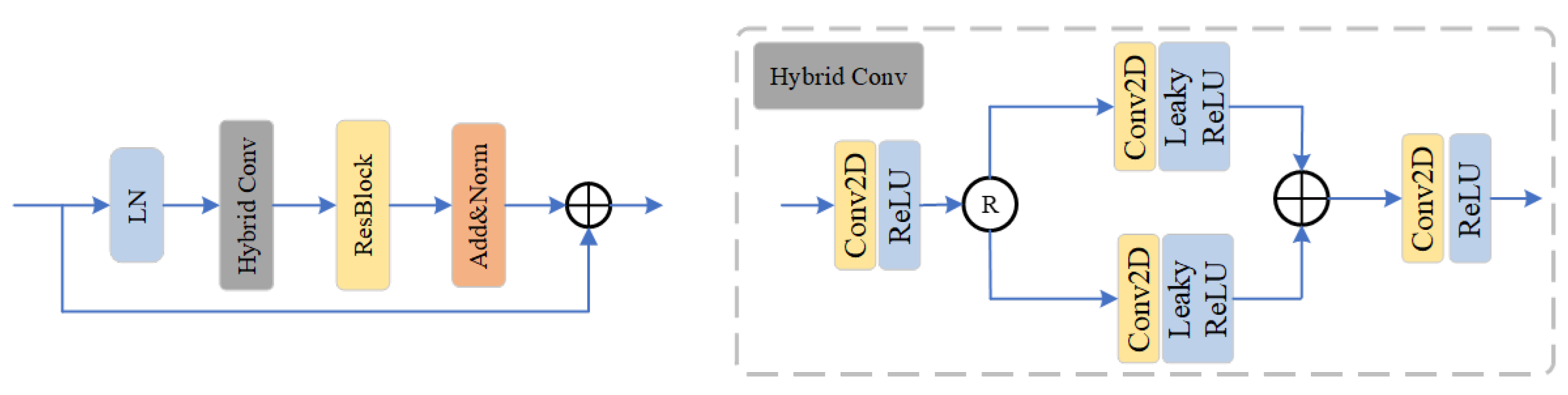
3.2. Blur Kernel Denoise Prior

HSIs denoising constitutes an ill-posed challenge that necessitates the incorporation of additional priors, or regularization, to appropriately constrain the reconstruction process, which traditional approaches strive to address by manually designing intricate regularization terms such as total variation (TV), sparsity, and low-rank constraints. Consequently, the effectiveness of these algorithms is largely contingent upon the capability of the designed priors to accurately represent the observed data. In the context of the HSIs super-resolution problem, it becomes imperative to efficiently leverage the intrinsic characteristics of HSIs, which include nonlocal self-similarity within the spatial domain and a high degree of correlation across spectral bands [45].

To address the limited sample size in hyperspectral imaging, the U-Net architecture employs a symmetric U-shaped structure comprising contracting and expanding paths (Figure 2). At the downsample stage, the contracting path progressively doubles the number of convolutional kernels at each level to expand feature channels, formulated as follows, where learnable kernels and b represent bias terms.

Global average pooling (GAP) follows each convolution to reduce feature map dimensions:

$$GAP\left(I\right),w_l=\left({\displaystyle \frac{1}{H^{\prime }{W}^{\prime }}}\right)\sum _{i=1}\sum _{j=1}{I}_{i,j},$$

(7)

the output of the downsampling process is the weight $w_l$ of the convolutional layer, which represents the learning of the hyperspectral image-blur kernel.

The upsampling process is achieved through deconvolution. The expanding path utilizes transposed convolution to progressively restore spatial resolution while halving channel numbers. Skip connections fuse multi-level features through concatenation

$$|I_{combined}=[I_{down};I_{up}],$$

(8)

integrating positional details from the contracting path with semantic abstractions from the expanding path.

The channel dimension follows exponential scaling: $C_{\iota }=2^l·C_0$ (contracting) and $C_l=2^{L-l}·C_0$ (expanding). Information compensation is quantified as

$$\Delta I=\sum _{l-1}{\alpha }_l·I_{skip}^l,$$

(9)

with ${\alpha }_l$ weighting skip-connection contributions. At the same time, after the intermediate layer ConvResnet (mixed residual convolution) further image-blur kernel extraction, through the layer-by-layer unsqueeze to achieve the size of the blur convolution kernel recovery, and the final output for the blur kernel after the BKPUnet network.

Figure 2. The Blur–Kernel–Prior Block-based U-Net.

Figure 2. The Blur–Kernel–Prior Block-based U-Net.

Based on the above description, the BKP module is designed wherein a U-Net architecture that serves as the foundational network of the proposed methodology, as depicted in Figure 2, and utilizes 3 × 3 convolutions with average pooling strategy as downsampling blocks with a stride of 2, while employing transposed convolutions as upsampling blocks alongside multiple layers functioning as feature extraction blocks. Meanwhile, ResNet with convolution-2D is chosen as the middle layer, learning abstract and sophisticated features. These feature extraction blocks are predicated on pointwise and 3 × 3 depthwise convolutions with a stride of 1, complemented by simple ReLU functions that are utilized as activation mechanisms. The final output is subsequently compared to the downsampled patches of the input blurry hyperspectral sub-images in conjunction with the learned blurry feature kernels. If the input sub-image $I_{in}^g\in {\mathbb{R}}^{{\displaystyle \frac{C}{G}}\times h\times w}$ and output sub-image $I_{out}^g\in {\mathbb{R}}^{{\displaystyle \frac{C}{G}}\times h\times w}$ are defined, and the downsampling process is represented as $\mathrm{Conv}-\mathrm{AvgPool}$, the upsampling process as $\mathrm{TransConv}$, and the intermediate layer as $\mathrm{ConvResNet}$, the overall process can be formalized as Equation (10),

$$\begin{array}{cc}\hfill I_{downsample}^g& =\mathrm{Conv}-\mathrm{AvgPool}{\left(I_{in}^g\right)}_P\hfill \\ \hfill I_{middle}^g& =\mathrm{TransConv}{\left(I_{downsample}^g\right)}_Q\hfill \\ \hfill I_{out}^g& =\mathrm{ConvResNet}{\left(I_{middle}^g\right)}_R\hfill \end{array}$$

(10)

while P, Q, R are layers of dowmsampler, middle, and upsampler.

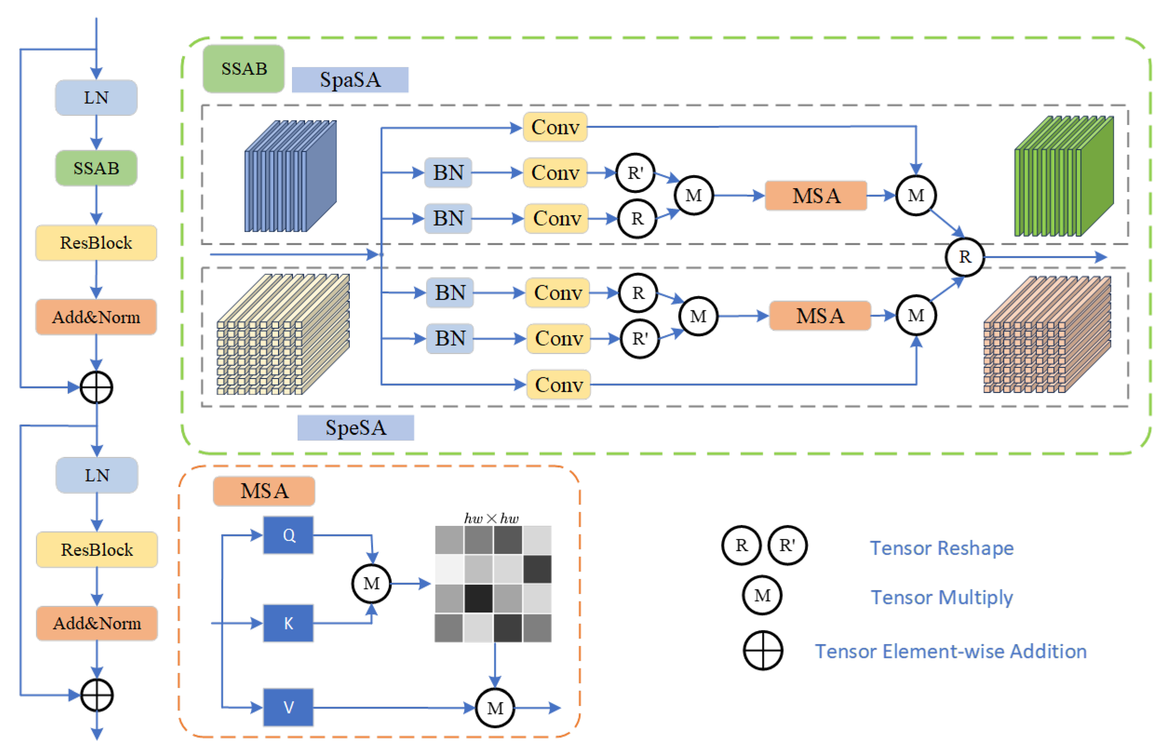
3.3. Spatial–Spectral Attention Feature Rebuild

To remove noise from HSIs, it is important to explore the similarity information in the spatial domain, which implies that similar pixels can be aggregated together for denoising. Existing deep-learning-based HSI denoising methods mainly utilize the convolutional layer to extract the local information with spatially invariant kernels, limiting the flexibility to model the nonlocal similarity. The Spatial–Spectral Attention (SSA) is specifically designed as an adaptive channel feature extraction mechanism within the network illustrated by SSPSR [44], with its structure shown in Figure 3. This module begins with layer normalization (LN) and enters the spatial–spectral Attention Block (SSAB) to generate preliminary spectral feature maps.

HSIs is a three-dimensional cubic image whose rich and detailed spatial and spectral features can be effectively extracted using 2DCNN. When a 2D CNN is used directly, preprocessing of the original HSIs is required, which leads to a reduction in spectral dimensionality. On the other hand, 3D convolutions can directly take HSIs as the input to the network without the need for complex preprocessing, thereby allowing simultaneous extraction of both spatial and spectral features. However, 3D CNNs involve a larger number of parameters to be learned, which presents a limitation in terms of computational complexity. Given that there exists a significant amount of redundant information and noise in the HSIs spectral bands, simple 3D convolution alone does not yield optimal HSIC results. To address these issues, a hybrid 2D-3D convolution is proposed, which combines the 2D convolution, 3D convolution, and residual mechanism of the harvester, effectively mitigating the deficiencies in feature extraction and enhancing computational efficiency. The Shallow spatial–spectral Attention Block (SSSAB) applies attention mechanisms separately to the spatial and spectral dimensions, aggregating contextual information from each patch in the spatial dimension while adaptively learning key information from each channel in the spectral dimension, selectively emphasizing relevant spectral features while suppressing irrelevant ones.

Many studies have proposed spectral attention-based methods for HSIs restoration and fidelity enhancement by leveraging spectral correlations [30,31]. However, standard transformers typically aggregate similar features based on global query-key pairs, which can result in the interaction of unrelated information, potentially interfering with the restoration outcomes. To overcome this disadvantage, stimulated by NLP [46,47], Spectral Similarity Attention (SpeSA) and Spatial Similarity Attention (SpaSA) mechanism-based multi-head attention are a replacement for the traditional spectral attention method.

In detail, SpeSA and SpaSA address these challenges through co-optimized spectral reliability weighting and spatial geometry-aware regularization, enabling physics-informed disentanglement of degradation factors, which adaptively score the similarity of features, retaining the relevant components while discarding the irrelevant ones, thereby preventing the interference of redundant information during the information interaction process. Considering $X\in {\mathbb{R}}^{C\times W·H}$ is HSIs contractive feature at spectral dimension and $X^{\prime }\in {\mathbb{R}}^{C·W\times C·H}$ is HSIs contractive feature at spatial dimension, MSA processes can be represented as Equation (11),

$$\mathrm{SpeSA}(Q,K,V)=\mathrm{SoftMax}\left(\sum _{m=1}^n\left({\mathrm{T}}_K^m\left({\displaystyle \frac{Q{K}^{\top }}{\sqrt{d}}}\right)\right)\right)V$$

(11)

where d is the feature dimension, and $T^m$ is the token studied by the feature. Then spectral features are learned by

$${\mathbf{F}}_{\mathbf{spe}}=ReLU\left({\mathbf{W}}_2\delta \left({\mathbf{W}}_1\mathrm{SpeSA}\right)\right),$$

(12)

where $W_1\in {\mathbb{R}}^{C\times C/r}$ and $W_2\in {\mathbb{R}}^{C\times C/r}$ form a bottleneck structure with reduction ratio r, $\delta$ denotes ReLU activation, and $ReLU(·)$ represents the ReLU nonlinear function.

Meanwhile, the position-aware attention is computed through affinity matrices,

$$e_{ij}={\displaystyle \frac{exp\left(\varphi {\left(\mathbf{y}\right)}^T\psi \left({\mathbf{y}}_j\right)\right)}{{\sum }_{j=1}^{N}exp\left(\varphi {\left({\mathbf{y}}_i\right)}^T\psi \left({\mathbf{y}}_j\right)\right)}},$$

(13)

where $\varphi (·)$ and $\psi (·)$ are linear projections of the input features and denote spatial positions. The refined features are obtained through,

$${\mathbf{F}}_{\mathbf{spa}}=\sum _{j=1}^N{e}_{ij}\theta \left(y_j\right),$$

(14)

Finally, the spectral and spatial streams are combined through element-wise multiplication,

$${\mathbf{F}}_{\mathbf{output}}={\mathbf{F}}_{\mathbf{spe}}\odot {\mathbf{F}}_{\mathbf{spa}}+{\mathbf{F}}_{\mathbf{input}}$$

(15)

where ${\mathbf{F}}_{\mathbf{output}}$ represents the extractor of deep spatial and spectral features of HSIs, adding input features ${\mathbf{F}}_{\mathbf{input}}$ as a residual structure for avoiding the vanishing gradient problem and enable the network to train more layers efficiently.

The Deep Spatial–Spectral Attention Block (DSSAB), shown in Figure 4, compared to SSSAB, chooses a strategy including additional residual layers (ResBlock) and Multi-Linear Layers (MLP) to extract detailed information more comprehensively, such as edges, textures, and other features. Meanwhile, SpaSA and SpeSA are provided for global information restoration. After extracting features from all channels, this module extensively learns the most informative spectral features. SSA can simultaneously focus on detailed features in different spatial positions and different spectral channels, thus achieving the purpose of SSA and enhancing the robustness of HSI restoration.

3.4. Overall Loss Function

A large body of work has demonstrated the positive impact of $L_1$ and $L_2$ losses in image restoration tasks. Since the $L_2$ loss usually leads to over-smoothed results, while the $L_1$ loss provides a more balanced error distribution and better convergence, the $L_1$ loss is employed to measure the accuracy of reconstructed images. $L_1$ loss calculates the pixel difference between the reconstructed $I_R$ HSIs and the original $I_{HR}$ HSIs, which can be formulated as Equation (16),

$${\mathcal{L}}_1(\Theta )={\displaystyle \frac{1}{N}}\sum _{n=1}^N\left|\right|H_{hr}^n-H_{sr}^n{\left|\right|}_1$$

(16)

where N is the number of images in the training batch, $\Theta$ denotes the parameter set of our proposed network, and $H_{hr}^n$ and $H_{sr}^n$ denote the nth reconstructed HSIs and the original HR HSIs, respectively. Although the $L_1$ loss can achieve good performance for natural images of SR, it ignores the spectral properties of HSIs and may lead to spectral distortion. SAM loss is introduced to maintain spectral consistency and spatial details. SAM loss can be formulated as Equation (17),

$${\mathcal{L}}_{spe}(\Theta )={\displaystyle \frac{1}{N}}\sum _{n=1}^N{\displaystyle \frac{1}{\pi }}arccos\left({\displaystyle \frac{H_{hr}^n·H_{sr}^n}{parallel{H}_{hr}^n{\Vert }_2·{\Vert H_{sr}^n\Vert }_2}}\right)$$

(17)

Furthermore, to measure the loss of informativeness of the blurred degraded HSIs, a peak signal-to-noise ratio loss PSNR [48] is introduced as Equation (18),

$${\mathcal{L}}_{PSNR}(\Theta )={\displaystyle \frac{1}{MN}}\sum _{i=1}^M\sum _{j=1}^{N}lo{g}_{10}\left({\displaystyle \frac{RMSE\left(I_{i,j}^R,I_{i,j}^{HR}\right)}{max(I_{i,j}^R}}\right)$$

(18)

where $I_{i,j}^R$, $I_{i,j}^{HR}$ denote the spectral dimension information of the $t(i,j)$ coordinate point in space, and RMSE(·) denotes the root-mean-square error of the spectral information of a point on the original HSIs and the reconstructed image.

The total loss for training the proposed network can be expressed as Equation (19),

$${\mathcal{L}}_{\mathit{total}}(\Theta )={\mathcal{L}}_1+{\lambda }_1{\mathcal{L}}_{spe}+{\lambda }_2{\mathcal{L}}_{PSNR}$$

(19)

where ${\lambda }_1$ and ${\lambda }_2$ denote trade-off parameters with different losses. Specifically, ${\lambda }_1$ controls the weighting of the spectral term to avoid excessively large values, which would lead to an excessive focus on spectral similarity at the expense of spatial detail. Similarly, ${\lambda }_2$ controls the weight of the PSNR term to avoid oversharpening in the spatial and spectral structure. The combination of the above losses can achieve superior reconstruction performance in both spatial and spectral dimensions. As a rule of thumb, ${\lambda }_1$ is set to 0.5 and ${\lambda }_2$ to 0.1 [31].

4. Results

To conduct a rigorous evaluation of the proposed method, several related approaches are selected for comparison, including the Singular Value Decomposition (SVD) [16], which epitomizes classic machine-learning techniques for deblur, alongside FPNSR [49], CEGATSR [50], which represent a classic CNN network, EUNet [45], MSDformer [31], and DSST [32], which are representative of novel deep-learning methodologies for denoise. In our model, as the application of group strategy, the number of bands processed by the spatial–spectral attention module was configured to be 32. Additionally, the batch size was designated as 32, and the patch size was set to 4. All methods are trained to utilize the PyTorch 2.1.0 framework, which was implemented on a graphics processing unit (GPU) employing an NVIDIA RTX 4090. Furthermore, the aforementioned methods underwent training for a total of 300 epochs. All deep-learning-based methods are trained and tested under the same conditions to ensure fairness.

4.1. Data Description

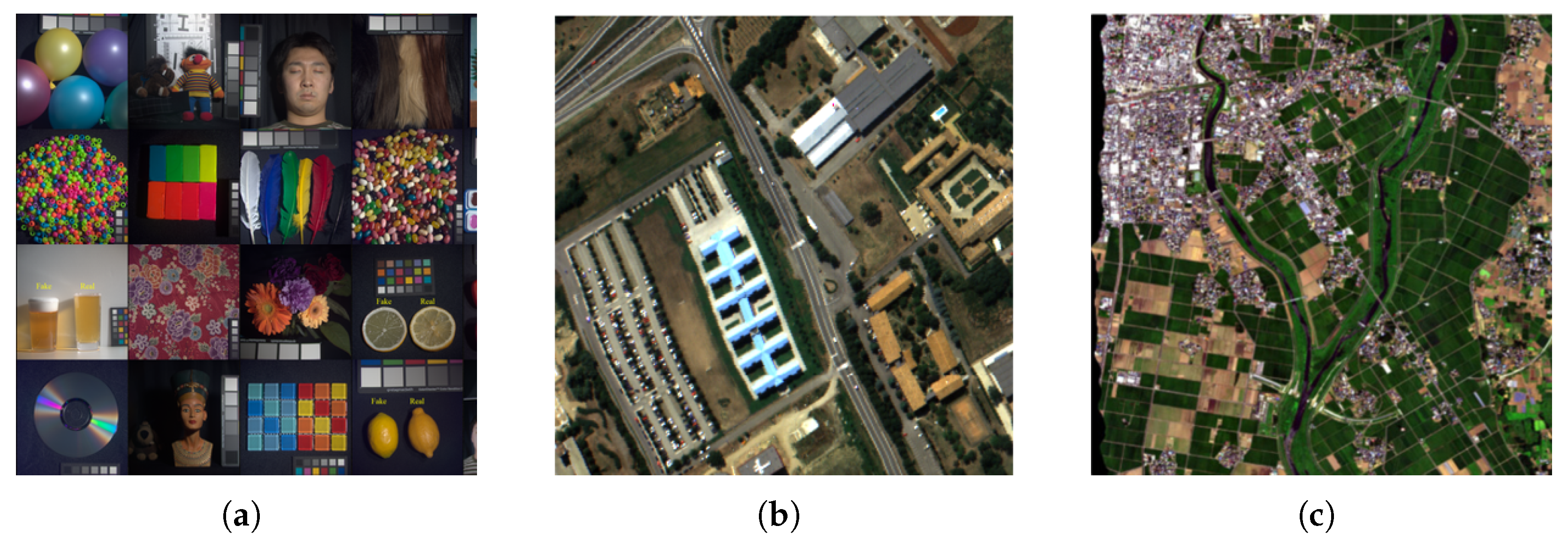
As illustrated in Figure 5, three publicly available HIS datasets, namely the CAVE, Chikusei, and Pavia University standard datasets, and an actual hyperspectral remotely sensed image dataset named the XiongAn dataset are used in the experiment as illustrated in Figure 6.

To systematically evaluate algorithm robustness, we established a hybrid degradation model combining parameterized blur types. The synthetic input generation process is formulated as

$$Kernel={\mu }_1·G_{\sigma }+{\mu }_2·M_{\theta ,\Delta x}({\mu }_1+{\mu }_2=1),$$

(20)

In our simulation experiments, a publicly available dataset is utilized, from which sub-images with a spatial resolution of 256 × 256 pixels are extracted. To generate the input for the low spatial resolution blurred HSIs, images are applied of a motion blur with random image shifts ranging from 0 to 20 pixels and rotations from 0 to 0.5 radians, along with a Gaussian blur characterized by a mean of 0 and a standard deviation of 3. This resulted in blurred images with average signal-to-noise ratio (SNR) gradients of 20 dB, 30 dB, and 40 dB. For the training set, 1000 sub-images are selected, while 200 sub-images are chosen for the validation and test sets from each of the CAVE, Chikusei, and Pavia University datasets. In all experiments conducted in this study, several evaluation metrics are employed: spectral angular similarity (SAM), peak signal-to-noise ratio (PSNR), global normalized loss (ERGAS), root-mean-square error (RMSE), structural similarity index (ASSIM), and cross-correlation (CC). Additionally, the model size, including reference model size and model parameters, was considered to assess the ease of deployment and migration of the model. Furthermore, ablation experiments are provided on the XiongAn dataset to demonstrate the importance of each module in enhancing model accuracy.

4.1.1. Cave Dataset

This contains 32 HSIs with a size of 512 × 512 and 31 spectral bands. In addition, each HSI also has a corresponding RGB image of size 512 × 512 and three spectral bands. This simulated dataset somehow characterizes the blurred features of the feature HSIs as well as the HSIs with a medium number of bands [51].

4.1.2. Pavia University Dataset

The Pavia University dataset [52] was acquired by the Reflectance Optical System Imaging Spectrometer (ROSIS) over the city center of Pavia in northern Italy. The HSIs in this dataset cover the wavelength range from 430 nm to 860 nm and are divided into 102 bands after removing the noise bands. The spatial resolution of the dataset is 1.3 m per pixel, and the image size is 1096 × 1096 pixels.

4.1.3. Chikusei Dataset

The Chikusei dataset [53] captures a variety of urban and agricultural landscapes in the Chikusei region of Ibaraki Prefecture, Japan. The dataset covers the wavelength range from 363 nm to 1018 nm with 128 spectral bands. Each image has a high spatial resolution of 2048 × 2048 pixels. These images cover different scenes, including urban areas, rice fields, forests, and roads, making them suitable for various remote sensing applications.

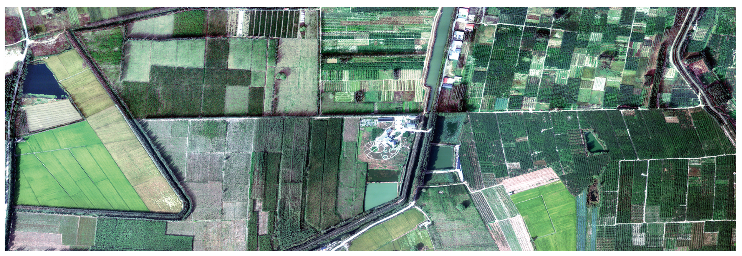
4.1.4. XiongAn Dataset

Including HSIs data of Horseshoe Bay Village in Xiong’an New Area (https://www.ygxb.ac.cn/zh/article/doi/10.11834/jrs.20209065/, accessed on 23 March 2025), collected by the full-spectrum multi-modal imaging spectrometer of the aerial system developed by the Shanghai Institute of Physics and Technology of the Chinese Academy of Sciences, with a spectral range of 400–1000 nm, 250 bands, and an image size of 3750 × 1580 pixels, with a spatial resolution of 0.5 m. The simultaneous field research on the distribution of land types is also conducted on 19 species.

4.2. Evaluation Metrics

To quantitatively evaluate the performance of the proposed method and the existing methods, six commonly used HSI reconstruction metrics are chosen. Let $I_{sol}$ and $I_{res}$ denote the denoised and super-resolution reconstructed HSIs and the reference HSIs, respectively.

4.2.1. Spectral Angle Mapping (SAM)

Spectral Angle Mapper (SAM) [54] is a technique used for HSI similarity on spectral dimension. In SAM, the spectrum of each pixel is considered to be a multidimensional vector (each band corresponds to one dimension), and then the angle between these vectors is calculated. Obviously, the closer the spectral angle between two spectra is to 0° indicates better similarity. The calculation formula is as Equation (21),

$$\mathrm{SAM}\left(I_{sol},I_{ref}\right)=arccos\left({\displaystyle \frac{I_{sol}·I_{ref}}{\Vert I_{sol}{\Vert }_2{\Vert I_{ref}\Vert }_2}}\right)$$

(21)

4.2.2. Root-Mean-Square Error (RMSE)

The Root-Mean-Square Error (RMSE) between spectral signals is a useful metric of the difference between two spectral signals. It is the square root of the mean of the sum of the squares of the differences between the observed and true values. When processing HSIs or analyzing spectral data, RMSE can be used to assess the quality of reconstructed spectra, compare the similarity between different spectra, or verify the accuracy of model predictions. The formula is as Equation (22),

$$\mathrm{RMSE}\left(\begin{array}{c}{I}_{sol},x_{ref}\end{array}\right)={\displaystyle \frac{\Vert I_{sol},I_{ref}{\Vert }_F}{\sqrt{n\times l}}}$$

(22)

where $\left|\right|·{\left|\right|}_F$ denotes the Frobenius paradigm. The optimal RMSE is 0.0.

In practice, the RMSE provides a quantitative metric for evaluating the differences between two spectral signals, but it does not provide information about the source of those differences. For example, a larger RMSE may be due to a difference in overall signal intensity or a small but significant difference at a specific wavelength. Therefore, RMSE is often used in conjunction with other analytical methods to gain a more complete understanding.

4.2.3. Peak Signal-to-Noise Ratio (PSNR)

The Peak Signal-to-Noise Ratio (PSNR) [48] of a spectral signal is a significant metric of the quality of HSI reconstruction, for example, to assess the degree of distortion between a compressed image and the original image. The PSNR is calculated by comparing the maximum possible power of the signal to the noise power of the signal and is usually expressed in decibels (dB) units. The calculation formula is as Equation (23),

$$\mathrm{PSNR}\left(I_{sol},I_{ref}\right)={\displaystyle \frac{1}{l}}\sum _{i=1}^l\left[10lo{g}_{10}\left({\displaystyle \frac{max\left(I_{sol}^i\right)}{RMSE\left(I_{sol}^i,I_{ref}^i\right)}}\right)\right]$$

(23)

PSNR is a useful metric for evaluating the quality of image reconstruction, reflecting sensor-perceived differences. the higher the PSNR value, the better the quality.

4.2.4. Structural Similarity Index (SSIM)

Structural Similarity Index (SSIM) [48] for spectral signals is a metric of similarity between two images that takes into account three aspects of similarity: luminance, contrast, and structure. SSIM is widely used in the image processing field to assess the quality of an image. Although SSIM was originally designed for images, it can also be applied to spectral signals to assess the similarity between two HSIs on the spatial dimension. The calculation formula is as Equation (24),

$$\mathrm{SSIM}\left(I_{sol},I_{ref}\right)={\displaystyle \frac{\left(2{\mu }_{I_{sol}}{\mu }_{I_{ref}}+C_1\right)\left(2{\sigma }_{I_{sol}{I}_{ref}}+C_2\right)}{\left({\mu }_{I_{sol}}^2+{\mu }_{I_{ref}}^2+C_1\right)\left({\sigma }_{I_{sol}}^2+{\sigma }_{I_{ref}}^2+C_2\right)}}$$

(24)

where ${\sigma }_{I_{sol}{I}_{ref}}$ denotes the covariance between $I_{sol}$ and $I_{ref}$. The optimal value of SSIM is 1.

4.2.5. Erreur Relative Globale Adimensionnelle de Synthèse (ERGAS)

ERGAS (Erreur Relative Globale Adimensionnelle de Synthèse [55], Integrated Relative Global Error) is a metric commonly used to assess the quality of hyperspectral data or image fusion. ERGAS is commonly used in remote sensing, especially in HSI processing, to evaluate the performance of image fusion, compression, or other processing techniques. The calculation formula is as Equation (25),

$$\mathrm{ERGAS}\left(I_{sol},I_{ref}\right)=100{\displaystyle \frac{1}{{\gamma }^2}}\sqrt{{\displaystyle \frac{1}{l}}\sum _{i=1}^l\left({\displaystyle \frac{\mathrm{RMSE}\left(I_{sol}^i,I_{ref}^i\right)}{{\mu }_i}}\right)}$$

(25)

where ${\mathrm{RMSE}}^i$ denotes the RMSE between $I_{sol}$ and $I_{res}$ in the i-th spectral band, and $\gamma$ is the scaling factor. The optimal ERGAS is 0.0.

4.2.6. Cross-Correlation (CC)

In hyperspectral data analysis, cross-correlation [56] is a metric of the similarity of two signals at different time displacements. For HSIs, in order to distinguish between spatial dimension and spectral dimension loss, this usually means comparing the image similarity in the same band and comparing the similarity between two bands; this is also known as Spatial Cross-correlation and Spectral Cross-correlation. The formula is as per Equation (26),

$$\begin{array}{c}{\mathrm{CC}}_{spa}(I_{sol},I_{ref})={\displaystyle \frac{1}{l}}{\displaystyle \sum _{i=1}^l}{\displaystyle \frac{\sum _{j=1}^n\left(I_{sol}^j-{\mu }_{I_{sol}}\right)\left(I_{ref}^j-{\mu }_{I_{ref}}\right)}{\sqrt{\sum _{j=1}^n{\left(I_{sol}^j-{\mu }_{I_{sol}}\right)}^2{\left(I_{ref}^j-{\mu }_{I_{ref}}\right)}^2}}}\\ {\mathrm{CC}}_{spe}\left(l_{sol},l_{ref}\right)={\displaystyle \frac{1}{mn}}{\displaystyle \sum _{i=1}^m}{\displaystyle \sum _{j=1}^n}{\displaystyle \frac{\sum _{j=1}^n\left(l_{sol}^{ij}-{\mu }_{l_{sol}}\right)\left(l_{ref}^{ij}-{\mu }_{l_{ref}}\right)}{\sqrt{\sum _{j=1}^n{\left(l_{sol}^{ij}-{\mu }_{l_{sol}}\right)}^2{\left(l_{ref}^{ij}-{\mu }_{l_{ref}}\right)}^2}}}\end{array}$$

(26)

4.2.7. Model Scale

Model size typically refers to the storage space requirements of the model, usually expressed in units such as bytes (Bytes), kilobytes (KB), or megabytes (MB). It primarily depends on the number of parameters in the model and the storage format of these parameters (e.g., floating-point numbers (FLOPs), integers, etc.). The model size directly affects storage requirements and computational resources, especially when deploying to edge devices or mobile devices.

The number of parameters, also known as computational complexity, characterizes the number of layers in the model and the number of neurons in each layer, which directly influence the parameter count. Generally, more parameters indicate stronger expressive capability of the model but may lead to increased demands for computational resources and energy consumption, which can, in turn, result in slower training and inference speeds as well as higher storage requirements. These challenges make it difficult to deploy such models on resource-constrained devices. Therefore, when designing a model, it is essential to strike a balance between the model’s accuracy and its reasonable scale, ensuring that the model remains efficient and practical for deployment without compromising its performance.

4.3. Comparison with State-of-the-Art HSIs Reconstruction Method

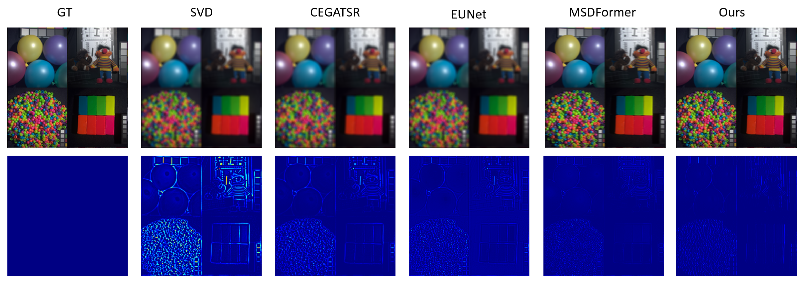
4.3.1. Experiments on the Cave Dataset

Table 1. Quantitative evaluation of different blur HSI reconstruction methods on the Cave dataset. The best and second-best results are bolded and underlined, respectively.

Method	Noise SNR	PSNR↑	SSIM↑	SAM↓	CC↑	RMSE↓	ERGAS↓
SVD		41.0335	0.9126	3.8944	0.9025	0.0308	5.3216
FPNSR		42.6521	0.9207	3.6567	0.9212	0.0238	3.1894
CEGATSR		45.6018	0.9265	3.1517	0.9304	0.0201	2.5681
EUNet	40 dB	47.0216	0.9480	2.8912	0.9411	0.0156	1.9260
MSDformer		48.0500	0.9610	2.2365	0.9698	0.0102	1.5724
DSST		48.3570	0.9660	2.0951	0.9661	0.0098	1.5654
Ours		49.5379	0.9701	2.0015	0.9764	0.0071	1.3256
SVD		32.5610	0.9027	3.8691	0.8712	0.0575	4.2561
FPNSR		35.4107	0.9100	3.3568	0.8998	0.0452	3.9430
CEGATSR		35.7075	0.9271	3.0176	0.9008	0.0399	3.6508
EUNet	30 dB	36.5417	0.9365	2.9315	0.9106	0.0368	3.2654
MSDformer		40.2125	0.9459	2.7776	0.9170	0.0304	2.9969
DSST		39.8931	0.9441	3.0014	0.9246	0.0347	2.8469
Ours		41.0015	0.9503	2.8958	0.9321	0.0211	2.3673
SVD		31.2659	0.8164	5.0918	0.8565	0.0899	7.7517
FPNSR		33.0023	0.8801	4.2019	0.8797	0.0765	6.6162
CEGATSR		33.3654	0.8834	4.0025	0.8865	0.0715	5.5681
EUNet	20 dB	34.2611	0.9068	3.9897	0.8944	0.0560	5.0007
MSDformer		35.5610	0.9227	3.6613	0.9017	0.0454	4.2526
DSST		36.0021	0.9296	3.3218	0.9065	0.0488	4.0524
Ours		37.0147	0.9403	3.1994	0.9169	0.0450	3.9367

presents the quantitative results of our proposed method alongside other comparative methods on the Chikusei dataset at different blurred noise signal-to-noise ratios (SNRs), with the best results highlighted in bold. The CAVE dataset, characterized by its rich spatial information, falls under the category of close-range hyperspectral imaging. Our model consistently outperforms other methods at blurred noise SNRs of 40 dB, 30 dB, and 20 dB across all six evaluation metrics. This indicates the robustness and effectiveness of the proposed method in handling various noise levels in HSI reconstruction. Figure 7 displays the qualitative results of HSIs reconstruction on the CAVE dataset at a 30 dB blurred noise SNR. Specifically, channels 31, 14, and 4, selected as the R-G-B channels, are shown to enhance visualization. While the Singular Value Decomposition (SVD) method can perform the reconstruction task, its performance is limited in terms of the recovery of fine spatial and spectral details. Although methods like EuNet and MSDformer demonstrate significant improvements in reconstruction quality, as observed in the red-boxed image, the BKPSSA model achieves superior pixel-level recovery results. The visual comparison highlights the effectiveness of BKPSSA in preserving both spatial and spectral information, resulting in more accurate and sharper reconstructed images. This further emphasizes the advantage of the proposed BKPSSA approach, which not only provides superior quantitative performance but also ensures better visual fidelity in the reconstructed HSIs, even under different levels of noise interference. The combination of advanced spatial–spectral feature extraction and noise suppression mechanisms allows BKPSSA to outperform existing methods in both objective metrics and subjective visual evaluation.

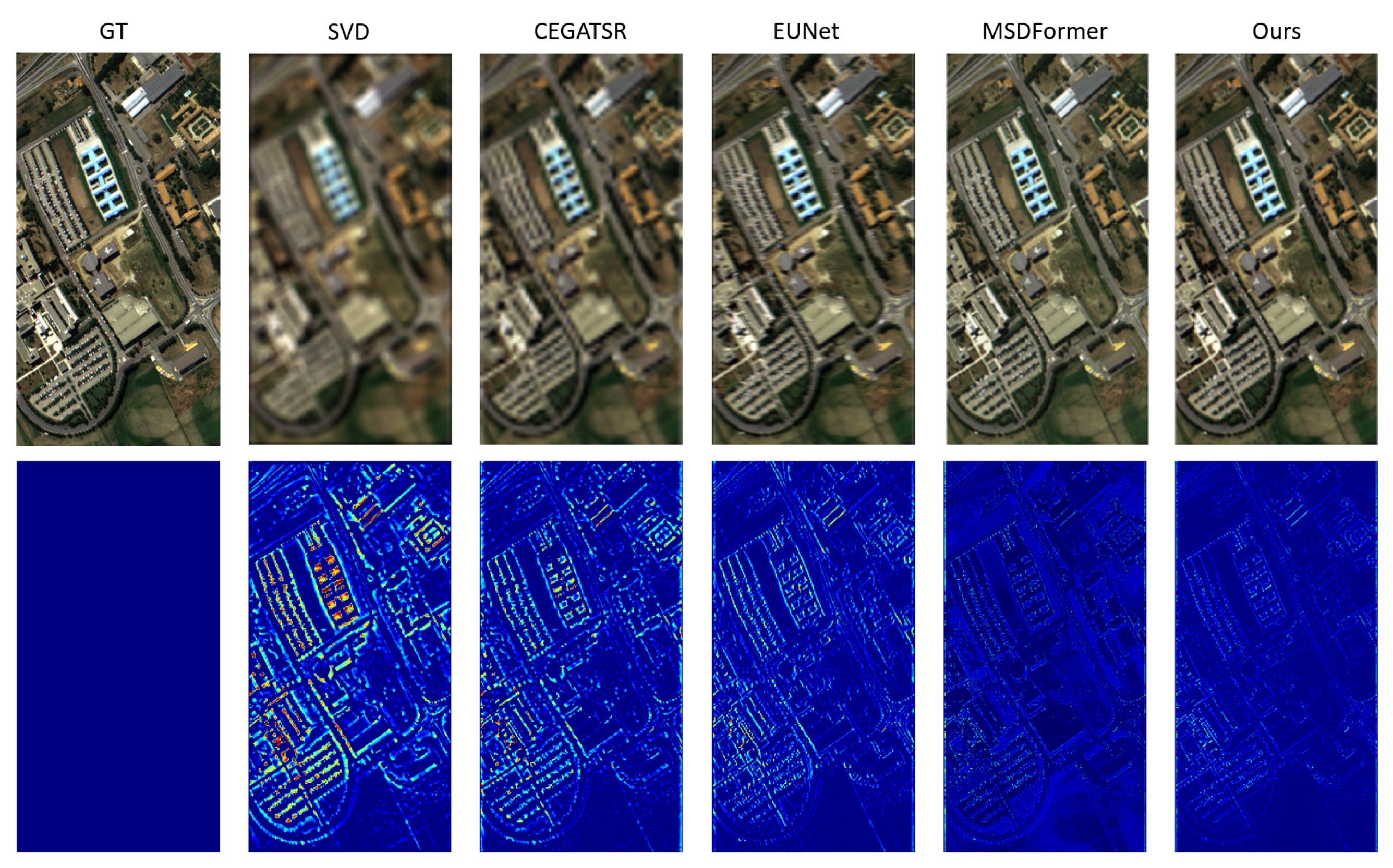
4.3.2. Experiments on the Pavia University Dataset

Table 2. Quantitative evaluation of different blur HSI reconstruction methods on the Pavia University dataset. The best and second-best results are bolded and underlined, respectively.

Method	Noise SNR	PSNR↑	SSIM↑	SAM↓	CC↑	RMSE↓	ERGAS↓
SVD		32.6901	0.9210	4.5464	0.9201	0.0509	3.9651
FPNSR		33.6158	0.9377	4.0107	0.9447	0.0452	3.2654
CEGATSR		34.4504	0.9405	3.9790	0.9564	0.0401	3.1145
EUNet	40 dB	35.1123	0.9499	3.7984	0.9650	0.0347	2.9897
MSDformer		35.8185	0.9511	3.6139	0.9744	0.0266	2.7710
DSST		35.6089	0.9597	3.5612	0.9781	0.0264	2.7798
Ours		36.0061	0.9602	3.5721	0.9790	0.0254	2.6066
SVD		24.6511	0.7677	5.2315	0.8210	0.0552	7.0056
FPNSR		25.4101	0.7758	4.9890	0.8526	0.0508	6.8709
CEGATSR		26.5140	0.7912	4.9208	0.8670	0.0432	6.6511
EUNet	30 dB	26.5964	0.7829	4.9085	0.8794	0.0401	6.1625
MSDformer		28.7894	0.8020	4.7797	0.8907	0.0379	5.9773
DSST		28.8975	0.8089	4.5120	0.8991	0.0397	5.7171
Ours		29.0017	0.8207	4.1711	0.9024	0.0335	5.4107
SVD		20.6841	0.6615	7.7978	0.7200	0.0779	9.9841
FPNSR		21.0564	0.6879	7.5009	0.7602	0.0705	9.6759
CEGATSR		21.6548	0.6977	7.2154	0.7877	0.0674	9.1555
EUNet	20 dB	21.8904	0.6954	7.0256	0.7889	0.0646	9.1606
MSDformer		22.6424	0.7069	6.6706	0.8001	0.0608	8.3564
DSST		23.1212	0.7102	6.5132	0.8115	0.0598	8.2356
Ours		23.5617	0.7256	6.0799	0.8210	0.0501	8.1979

presents the quantitative results of all methods on the Pavia University dataset across six evaluation metrics, expressed in terms of blurred noise signal-to-noise ratios (SNRs) of 40 dB, 30 dB, and 20 dB. Due to the limited number of training samples available in the Pavia University dataset, each method tends to perform poorly on this dataset in comparison to others, as smaller training sets often lead to overfitting or insufficient generalization. Nevertheless, the proposed BKPSSA method consistently achieves better results across all six evaluation metrics and at every level of blurred noise SNR compared to other methods. This demonstrates the robustness and efficiency of BKPSSA in handling noise and preserving image quality under different noise conditions. The experimental results further highlight that the BKPSSA method is particularly well-suited for scenarios involving small sample training datasets. Despite the challenges posed by the limited amount of training data, BKPSSA can effectively learn from the available samples by leveraging both local and global spatial–spectral information, along with prior noise knowledge. This combination allows the model to recover fine details in the HSIs while suppressing noise, even when the training data are sparse. By incorporating these advanced techniques, the proposed BKPSSA method provides strong robustness in both spatial and spectral dimensions, enabling high-quality HSI denoising and reconstruction. This capability is crucial for real-world applications where data may be limited, yet the need for accurate and reliable image reconstruction remains paramount. The ability of BKPSSA to effectively exploit available information, even with small datasets, underscores its potential for a wide range of HSI processing tasks. And Figure 8 shows the error of reconstructed images from different methods compared with the Ground Truth.

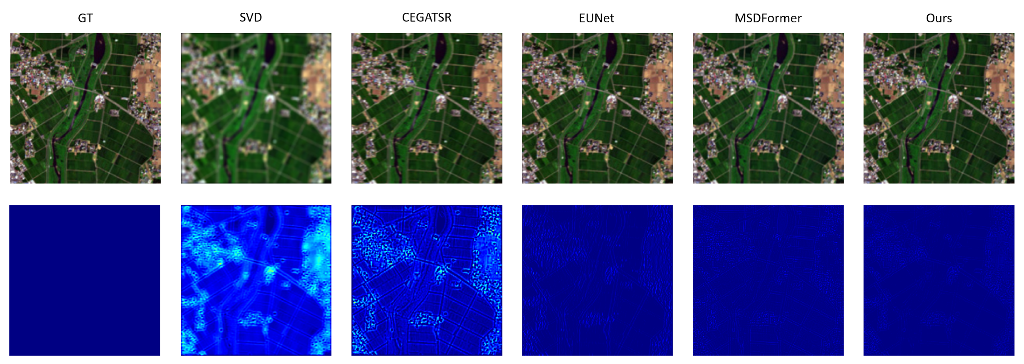
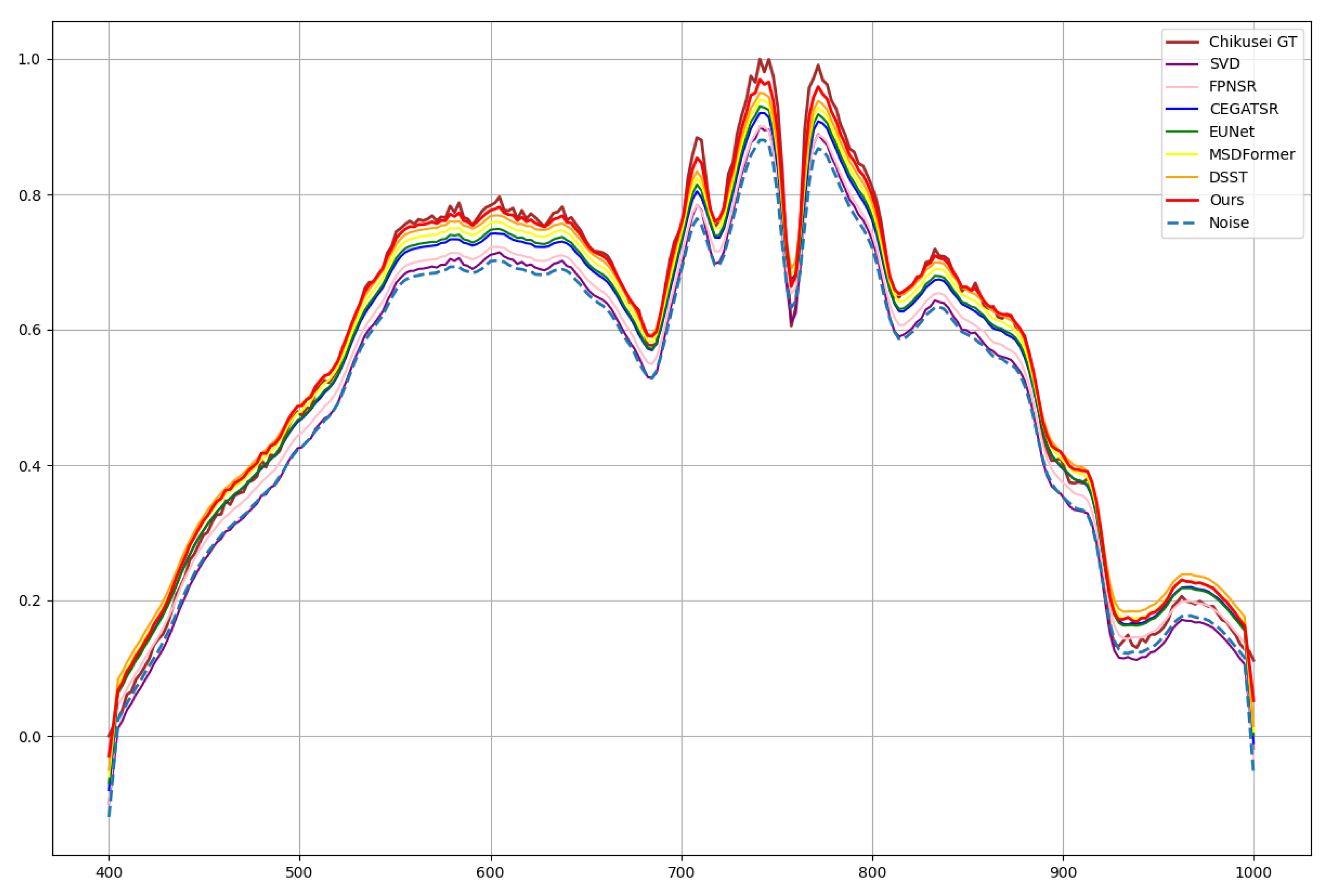
4.3.3. Experiments on the Chikusei Dataset

Table 3. Quantitative evaluation of different blur HSI reconstruction methods on the Chikusei dataset. The best and second-best results are bolded and underlined, respectively.

Method	Noise SNR	PSNR↑	SSIM↑	SAM↓	CC↑	RMSE↓	ERGAS↓
SVD		40.2125	0.9021	1.8880	0.9311	0.0399	6.5613
FPNSR		41.9690	0.9125	1.6510	0.9545	0.0213	5.6556
CEGATSR		41.3915	0.9360	1.2665	0.9601	0.0117	4.9001
EUNet	40 dB	42.8070	00.9290	1.6105	0.9726	0.0208	4.6324
MSDformer		47.2824	0.9722	1.1498	0.9800	0.0129	2.4315
DSST		47.5658	0.9801	1.2056	0.9811	0.0102	2.3001
Ours		48.5601	0.9821	1.1257	0.9852	0.0097	2.1871
SVD		30.2501	0.8871	2.9251	0.8210	0.0454	10.0235
FPNSR		32.0024	0.9015	2.8864	0.8599	0.0421	9.5001
CEGATSR		33.3871	0.9295	2.2665	0.8479	0.0397	8.9802
EUNet	30 dB	32.9207	0.9034	2.4098	0.8325	0.0315	9.1060
MSDformer		35.0911	0.9310	2.2914	0.8534	0.0256	8.9203
DSST		36.0091	0.9541	2.6050	0.8736	0.0212	8.7215
Ours		38.6061	0.9544	2.7281	0.8834	0.0201	7.9957
SVD		22.5640	0.8012	5.4689	0.7921	0.0932	12.0309
FPNSR		24.0545	0.8211	4.6507	0.8172	0.0804	11.8907
CEGATSR		25.6849	0.8263	4.4190	0.8410	0.0826	11.5119
EUNet	20 dB	24.9102	0.8362	4.5023	0.8349	0.0751	11.0029
MSDformer		25.5914	0.8402	4.2531	0.8563	0.0699	10.5203
DSST		25.9014	0.8415	4.1989	0.8623	0.0665	10.4911
Ours		28.0651	0.8521	4.7215	0.8590	0.0601	10.0718

presents the quantitative results of our method compared to other approaches on the Chikusei dataset under different levels of blurry SNR. The best results are highlighted in bold, while the second-best results are underlined. It is noteworthy that the SVD, a non-deep-learning method, demonstrates average denoising and reconstruction performance and struggles with nonlinear blurry noise. In contrast, deep-learning methods show significant improvements.

The FPNSR and CEGATSR methods utilize grouping strategies to extract spectral information, achieving better super-resolution (SR) results than SVD. The MSDformer builds upon the grouping strategy by incorporating a Transformer to capture long-range dependencies in spectral information; however, it lacks attention to local spatial details. Notably, our proposed BKPSSA captures global spatial–spectral dependencies, demonstrating superior spatial–spectral information extraction and fusion capabilities, outperforming other methods across all metrics, regardless of the scaling factor at 40 dB, 30 dB, or 20 dB.

Figure 9 provides visualizations of the HSIs reconstructions from the Chikusei test set at a 30 dB blurry noise SNR. Channels 20, 40, and 60 are selected for RGB visualization to enhance visual interpretation. It is evident that while the SVD method performs SR on the HSIs, it results in the blurriest edges and poorest smooth region reconstructions. Eunet and MSDformer show improved reconstructions, especially regarding line details, but still have deficiencies in detail recovery. In contrast, our BKPSSA achieves superior edge and detail restoration.

4.3.4. Comprehensive Evaluation in the XiongAn Database

The XiongAn dataset was selected as the real data to test the network’s robustness.

Table 4. Comparisons of the Parameters, FLOPs on the XiongAn Dataset.

		FPNSR	CEGATSR	EUNet	MSDformer	DDST	Ours
Parameters		4.42 M	13.55 M	12.83 M	14.90 M	20.65 M	12.77 M
FLOPs		5.762 G	29.925 G	16.613 G	53.915 G	59.34 G	38.89 G
PSNR↑		33.1614	34.0316	34.9877	35.0235	35.6724	36.9011
SSIM↑		0.9001	0.9102	0.9125	0.9271	0.9235	0.9460
SAM↓		3.5652	3.4540	3.1654	3.1027	3.0562	2.8965
CC↑		0.8985	0.9022	9.9075	0.9108	0.9156	0.9279
RMSE↓		0.0204	0.0299	0.0285	0.0256	0.0244	0.0217
ERGAS↓		5.4510	5.3021	5.3654	5.2347	5.2194	5.2024

shows the model sizes and evaluation metrics within the XiongAn dataset. Specifically, our proposed BKPSSA achieved the highest scores across all metrics, convincingly demonstrating its excellent ability to restore spatial details and preserve spectral features. MSDFormer and DSST also exhibited good spectral reconstruction capabilities but still lagged behind DL-based methods in the spatial domain. The matrix-based method, SVD, suffered from severe distortion, leading to a loss of spatial details and spectral features.

On the other hand, in terms of model size, our proposed BKPSSA has a moderate number of FLOPs and achieves better reconstruction performance with a lower number of parameters. Figure 10 shows the visual results from the XiongAn dataset. We can see that methods such as CEGATSR, EuNet, and MSDFormer exhibit noticeable distortions, highlighting their limited capability in the reconstruction domain. BKPSSA, on the other hand, produces more satisfactory results with fewer artifacts.

In summary, after comparing different deblurring algorithms applied to hyperspectral images, most of the CNN and Attention-based methods of reconstruction on deblur rely on the assumption that the spectral and spatial degradation lie on the resolution. As a result, shown in Figure 11, the spectral details are smoothed out based on traditional methods, and even if the signal-to-noise ratio is improved, it cannot be directly used to remove the blurred noise.

5. Discussion

In this section, the effect of different modules is reported on the robustness performance of different models on more subdivided scale blur noise and the effectiveness of the different modules of the proposed BKPSSA.

5.1. Comparison of Robustness Performance of Different Models at a More Subdivided Noise Scale

Based on the above model comparison, the blur noise is set from 20 to 40 dB to a more detailed scale, and a single dataset is trained and tested at 5 dB intervals. The results are shown in Figure 12, and the evaluation indicators are PSNR and SAM. It can be seen that on the Chikusei and CAVE datasets, the proposed BKPSSA has better robustness, and when the noise level increases, the response is stable, and there is no mutation compared with other methods.

5.2. Effectiveness of the Grouping Strategy

At the beginning of the network, the spectral bands are divided into subgroups and efficiently extract the local spatial–spectral information. Since the grouping strategy was studied in depth and relevant effects of the different settings are analyzed in the experimental results of the research, the grouping processes have not been studied here but demonstrate the effectiveness of the grouping strategy. Models without grouping strategies are donated as w/o Groups and train the network in a band-by-band function. As a result, the complexity of the model increases as the number of spectral bands in the image increases, which reduces the efficiency of the network.

5.3. Effectiveness of the BKP Block

In the proposed a priori denoising module, BKP, a U-net-based neural network is employed to extract global noise features and decouple the input hyperspectral sub-image from the blurred kernel, thereby enhancing the model’s representation capability. To evaluate the effectiveness of the BKP module, a network composed entirely of CNN modules is designed. Specifically, the U-net network is replaced with the AE (Autoencode-decode) module [57], which is commonly used in deep learning. The values of all metrics deteriorate significantly, demonstrating the importance of the designed BKP. The Autoencode-decode network is denoted as “w/o AE” in

Table 5. Ablation experiments of some variants of the proposed method over the Chikusei dataset at SNR 30 dB. Bold represents the best.

Variant	Params/FLOPs	PSNR↑	SSIM↑	SAM↓	RMSE↓
w/o Groups	8.48 M/26.77 G	30.0291	0.8671	3.5689	0.0588
w/o AE	5.56 M/15.02 G	30.2401	0.8823	4.0905	0.0627
w/o SA1	7.81 M/18.65 G	31.5689	0.8564	3.6580	0.0460
w/o SA2	5.56 M/16.52 G	30.6522	0.9088	2.6512	0.0362
Ours	12.77 M/38.89 G	35.0911	0.9310	2.2914	0.0256

. While the AE module slightly preserves spectral similarity, the spatial similarity is severely degraded, which further justifies the significance of the proposed BKP.

5.4. Effectiveness of Spatial and Spectral Attention

In BKPSSA, Spatial and Spectral Attention (SSA) is designed to learn features from the spatial and spectral dimensions, respectively. To validate the effectiveness of the proposed SSA structure, various variants were designed using either spatial attention or spectral attention alone. As shown in Table 4, the performance of the model is significantly degraded when using “w/o Spatial Attention Only” (w/o SA1) or “Spectral Attention Only” (w/o SA2). The likely reason for this is that each module specializes in either spatial or spectral information, and their parallel operation enables the integration of information, facilitating the comprehensive learning of spatial and spectral features in the HSIs. When operating independently, significant shortcomings in the efficient extraction of spatial or spectral information arise, which fail to address the long-range dependencies of spatial information or the redundancy present in spectral information.

6. Conclusions

In this study, we propose a novel HSI deblurring reconstruction network, referred to as BKPSSA, to address the limitations of existing transformation-based methods in mitigating image-blur interference during HSI reconstruction. Specifically, BKPSSA is founded on a group strategy learning framework, wherein the BKP module is employed to establish prior knowledge of the blur kernel within the learned subspace, thereby restoring spatial consistency through the estimation of the blur kernel. The SSA module incorporates shallow spatial–spectral feature extraction based on a hybrid 2D-3D convolution mechanism alongside a spatial–spectral residual attention network based on multi-head attention, which effectively extracts global information. Extensive experiments on both natural and remote sensing images demonstrate that the proposed method outperforms other approaches in terms of visual perception and quantitative metrics. Additionally, ablation studies validate the effectiveness of each proposed module.

In future research, the proposed method will be further improved in aspect, which is to obtain prior noise information from the acquisition perspective and compare it with the network. Additionally, efforts will be made to reduce the parameter burden while ensuring high-quality reconstruction.

References

1. Tejasree, G.; Agilandeeswari, L. An extensive review of hyperspectral image classification and prediction: Techniques and challenges. Multimed. Tools Appl. 2024, 83, 80941–81038. [Google Scholar] [CrossRef]
2. Nie, X.; Xue, Z.; Lin, C.; Zhang, L.; Su, H. Structure-prior-constrained low-rank and sparse representation with discriminative incremental dictionary for hyperspectral image classification. IEEE Trans. Geosci. Remote Sens. 2024, 62, 5506319. [Google Scholar] [CrossRef]
3. Shu, Z.; Wang, Y.; Yu, Z. Dual attention transformer network for hyperspectral image classification. Eng. Appl. Artif. Intell. 2024, 127, 107351. [Google Scholar] [CrossRef]
4. Namburu, H.; Munipalli, V.N.; Vanga, M.; Pasam, M.; Sikhakolli, S.; Chinnadurai, S. Cholangiocarcinoma Classification using MedisawHSI: A Breakthrough in Medical Imaging. In Proceedings of the 2024 Second International Conference on Emerging Trends in Information Technology and Engineering (ICETITE), Vellore, India, 22–23 February 2024; pp. 1–6. [Google Scholar] [CrossRef]
5. Li, S.; Song, Q.; Liu, Y.; Zeng, T.; Liu, S.; Jie, D.; Wei, X. Hyperspectral imaging-based detection of soluble solids content of loquat from a small sample. Postharvest Biol. Technol. 2023, 204, 112454. [Google Scholar] [CrossRef]
6. Gong, M.; Jiang, F.; Qin, A.K.; Liu, T.; Zhan, T.; Lu, D.; Zheng, H.; Zhang, M. A spectral and spatial attention network for change detection in hyperspectral images. IEEE Trans. Geosci. Remote Sens. 2021, 60, 5521614. [Google Scholar] [CrossRef]
7. Petropoulos, G.P.; Kalivas, D.P.; Georgopoulou, I.A.; Srivastava, P.K. Urban vegetation cover extraction from hyperspectral imagery and geographic information system spatial analysis techniques: Case of Athens, Greece. J. Appl. Remote Sens. 2015, 9, 096088. [Google Scholar] [CrossRef]
8. Zia, A.; Zhou, J.; Gao, Y. Exploring chromatic aberration and defocus blur for relative depth estimation from monocular hyperspectral image. IEEE Trans. Image Process. 2021, 30, 4357–4370. [Google Scholar] [CrossRef]
9. Geladi, P.; Burger, J.; Lestander, T. Hyperspectral imaging: Calibration problems and solutions. Chemom. Intell. Lab. Syst. 2004, 72, 209–217. [Google Scholar] [CrossRef]
10. Gao, B.C.; Montes, M.J.; Davis, C.O.; Goetz, A.F. Atmospheric correction algorithms for hyperspectral remote sensing data of land and ocean. Remote Sens. Environ. 2009, 113, S17–S24. [Google Scholar] [CrossRef]
11. Jia, J.; Zheng, X.; Guo, S.; Wang, Y.; Chen, J. Removing stripe noise based on improved statistics for hyperspectral images. IEEE Geosci. Remote Sens. Lett. 2020, 19, 5501405. [Google Scholar] [CrossRef]
12. Rasti, B.; Scheunders, P.; Ghamisi, P.; Licciardi, G.; Chanussot, J. Noise reduction in hyperspectral imagery: Overview and application. Remote Sens. 2018, 10, 482. [Google Scholar] [CrossRef]
13. He, H.; Cao, M.; Gao, Y. Noise learning of instruments for high-contrast, high-resolution and fast hyperspectral microscopy and nanoscopy. Nat. Commun. 2024, 15, 754. [Google Scholar] [CrossRef]
14. Jiang, T.X.; Zhuang, L.; Huang, T.Z. Adaptive hyperspectral mixed noise removal. IEEE Trans. Geosci. Remote Sens. 2021, 60, 1–13. [Google Scholar] [CrossRef]
15. Peng, J.; Sun, W.; Li, H.C.; Li, W.; Meng, X.; Ge, C.; Du, Q. Low-rank and sparse representation for hyperspectral image processing: A review. IEEE Geosci. Remote Sens. Mag. 2021, 10, 10–43. [Google Scholar] [CrossRef]
16. Guo, Q.; Zhang, C.; Zhang, Y.; Liu, H. An efficient SVD-based method for image denoising. IEEE Trans. Circuits Syst. Video Technol. 2015, 26, 868–880. [Google Scholar] [CrossRef]
17. Rasti, B.; Ghamisi, P.; Benediktsson, J.A. Hyperspectral mixed Gaussian and sparse noise reduction. IEEE Geosci. Remote Sens. Lett. 2019, 17, 474–478. [Google Scholar] [CrossRef]
18. Li, W.; Prasad, S.; Fowler, J.E. Hyperspectral image classification using Gaussian mixture models and Markov random fields. IEEE Geosci. Remote Sens. Lett. 2013, 11, 153–157. [Google Scholar] [CrossRef]
19. Wang, X.; Hu, Q.; Cheng, Y.; Ma, J. Hyperspectral image super-resolution meets deep learning: A survey and perspective. IEEE/CAA J. Autom. Sin. 2023, 10, 1668–1691. [Google Scholar] [CrossRef]
20. Han, X.H.; Shi, B.; Zheng, Y. SSF-CNN: Spatial and spectral fusion with CNN for hyperspectral image super-resolution. In Proceedings of the 2018 25th IEEE International Conference on Image Processing (ICIP), Athens, Greece, 7–10 October 2018; pp. 2506–2510. [Google Scholar] [CrossRef]
21. Wang, L.; Bi, T.; Shi, Y. A frequency-separated 3D-CNN for hyperspectral image super-resolution. IEEE Access 2020, 8, 86367–86379. [Google Scholar] [CrossRef]
22. Arun, P.V.; Buddhiraju, K.M.; Porwal, A.; Chanussot, J. CNN-based super-resolution of hyperspectral images. IEEE Trans. Geosci. Remote Sens. 2020, 58, 6106–6121. [Google Scholar] [CrossRef]
23. Dixit, A.; Gupta, A.K.; Gupta, P.; Srivastava, S.; Garg, A. UNFOLD: 3D U-Net, 3D CNN and 3D transformer based hyperspectral image denoising. IEEE Trans. Geosci. Remote Sens. 2023, 61, 5529710. [Google Scholar] [CrossRef]
24. Wang, Z.; Ng, M.K.; Zhuang, L.; Gao, L.; Zhang, B. Nonlocal self-similarity-based hyperspectral remote sensing image denoising with 3-D convolutional neural network. IEEE Trans. Geosci. Remote Sens. 2022, 60, 5531617. [Google Scholar] [CrossRef]
25. Hou, R.; Li, F. Hyperspectral image denoising via cooperated self-supervised CNN transform and nonconvex regularization. Neurocomputing 2024, 616, 128912. [Google Scholar] [CrossRef]
26. Shi, H.; Cao, G.; Zhang, Y.; Ge, Z.; Liu, Y.; Fu, P. H2A2 Net: A hybrid convolution and hybrid resolution network with double attention for hyperspectral image classification. Remote Sens. 2022, 14, 4235. [Google Scholar] [CrossRef]
27. Galassi, A.; Lippi, M.; Torroni, P. Attention in natural language processing. IEEE Trans. Neural Netw. Learn. Syst. 2020, 32, 4291–4308. [Google Scholar] [CrossRef]
28. Han, K.; Xiao, A.; Wu, E.; Guo, J.; Xu, C.; Wang, Y. Transformer in transformer. Adv. Neural Inf. Process. Syst. 2021, 34, 15908–15919. [Google Scholar]
29. Zhang, D.; Zhou, F. Self-supervised image denoising for real-world images with context-aware transformer. IEEE Access 2023, 11, 14340–14349. [Google Scholar] [CrossRef]
30. Zhao, Y.; Zhai, D.; Jiang, J.; Liu, X. ADRN: Attention-based deep residual network for hyperspectral image denoising. In Proceedings of the ICASSP 2020-2020 IEEE International Conference on Acoustics, Speech and Signal Processing (ICASSP), Barcelona, Spain, 4–8 May 2020; pp. 2668–2672. [Google Scholar] [CrossRef]
31. Chen, S.; Zhang, L.; Zhang, L. Msdformer: Multi-scale deformable transformer for hyperspectral image super-resolution. IEEE Trans. Geosci. Remote Sens. 2023, 61, 5525614. [Google Scholar] [CrossRef]
32. Yang, J.; Lin, T.; Liu, F.; Xiao, L. Learning degradation-aware deep prior for hyperspectral image reconstruction. IEEE Trans. Geosci. Remote Sens. 2023, 61, 5531515. [Google Scholar] [CrossRef]
33. Zhuang, L.; Ng, M.K.; Gao, L.; Michalski, J.; Wang, Z. Eigenimage2Eigenimage (E2E): A self-supervised deep learning network for hyperspectral image denoising. IEEE Trans. Neural Netw. Learn. Syst. 2023, 35, 16262–16276. [Google Scholar] [CrossRef]
34. Geng, P.; Zhang, M.; Li, X. Hyperspectral image deblurring based on joint utilization of spatial-spectral information. In Proceedings of the 2023 16th International Symposium on Computational Intelligence and Design (ISCID), Hangzhou, China, 16–17 December 2023; pp. 156–160. [Google Scholar] [CrossRef]
35. Fan, H.; Li, C.; Guo, Y.; Kuang, G.; Ma, J. Spatial–Spectral Total Variation Regularized Low-Rank Tensor Decomposition for Hyperspectral Image Denoising. IEEE Trans. Geosci. Remote Sens. 2018, 56, 6196–6213. [Google Scholar] [CrossRef]
36. He, W.; Zhang, H.; Zhang, L.; Shen, H. Total-variation-regularized low-rank matrix factorization for hyperspectral image restoration. IEEE Trans. Geosci. Remote Sens. 2015, 54, 178–188. [Google Scholar] [CrossRef]
37. Zhang, Q.; Zheng, Y.; Yuan, Q.; Song, M.; Yu, H.; Xiao, Y. Hyperspectral image denoising: From model-driven, data-driven, to model-data-driven. IEEE Trans. Neural Netw. Learn. Syst. 2023, 35, 13143–13163. [Google Scholar] [CrossRef] [PubMed]
38. Zhou, X.; Zhang, X.; Guo, P. Expected patch log likelihood with a prior of mixture of matrix normal distributions for image denoising. In Proceedings of the 2018 Ninth International Conference on Intelligent Control and Information Processing (ICICIP), Wanzhou, China, 9–11 November 2018; pp. 344–348. [Google Scholar] [CrossRef]
39. Mildenhall, B.; Barron, J.T.; Chen, J.; Sharlet, D.; Ng, R.; Carroll, R. Burst denoising with kernel prediction networks. In Proceedings of the IEEE Conference on Computer Vision and Pattern Recognition, Salt Lake City, UT, USA, 18–23 June 2018; pp. 2502–2510. [Google Scholar] [CrossRef]
40. Cai, J.; Zuo, W.; Zhang, L. Dark and bright channel prior embedded network for dynamic scene deblurring. IEEE Trans. Image Process. 2020, 29, 6885–6897. [Google Scholar] [CrossRef]
41. Xia, Z.; Perazzi, F.; Gharbi, M.; Sunkavalli, K.; Chakrabarti, A. Basis Prediction Networks for Effective Burst Denoising with Large Kernels. In Proceedings of the 2020 IEEE/CVF Conference on Computer Vision and Pattern Recognition (CVPR), Seattle, WA, USA, 13–19 June 2020; pp. 11841–11850. [Google Scholar] [CrossRef]
42. Liu, Y.; Hu, J.; Kang, X.; Luo, J.; Fan, S. Interactformer: Interactive transformer and CNN for hyperspectral image super-resolution. IEEE Trans. Geosci. Remote Sens. 2022, 60, 5531715. [Google Scholar] [CrossRef]
43. Hu, J.; Liu, Y.; Kang, X.; Fan, S. Multilevel progressive network with nonlocal channel attention for hyperspectral image super-resolution. IEEE Trans. Geosci. Remote Sens. 2022, 60, 5543714. [Google Scholar] [CrossRef]
44. Jiang, J.; Sun, H.; Liu, X.; Ma, J. Learning spatial-spectral prior for super-resolution of hyperspectral imagery. IEEE Trans. Comput. Imaging 2020, 6, 1082–1096. [Google Scholar] [CrossRef]
45. Liu, D.; Li, J.; Yuan, Q.; Zheng, L.; He, J.; Zhao, S.; Xiao, Y. An efficient unfolding network with disentangled spatial-spectral representation for hyperspectral image super-resolution. Inf. Fusion 2023, 94, 92–111. [Google Scholar] [CrossRef]
46. Cordonnier, J.B.; Loukas, A.; Jaggi, M. Multi-head attention: Collaborate instead of concatenate. arXiv 2020, arXiv:2006.16362. [Google Scholar] [CrossRef]
47. Hu, M.; Wu, C.; Zhang, L. GlobalMind: Global multi-head interactive self-attention network for hyperspectral change detection. ISPRS J. Photogramm. Remote Sens. 2024, 211, 465–483. [Google Scholar] [CrossRef]
48. Hore, A.; Ziou, D. Image quality metrics: PSNR vs. SSIM. In In Proceedings of the 2010 20th International Conference on Pattern Recognition, Istanbul, Turkey, 23–26 August 2010; pp. 2366–2369. [Google Scholar] [CrossRef]
49. Sun, H.; Zhong, Z.; Zhai, D.; Liu, X.; Jiang, J. Hyperspectral image super-resolution using multi-scale feature pyramid network. In Proceedings of the Digital TV and Wireless Multimedia Communication: 16th International Forum, IFTC 2019, Shanghai, China, 19–20 September 2019; Revised Selected Papers 16. Springer: Berlin/Heidelberg, Germany, 2020; pp. 49–61. [Google Scholar] [CrossRef]
50. Liu, C.; Dong, Y. CNN-Enhanced graph attention network for hyperspectral image super-resolution using non-local self-similarity. Int. J. Remote Sens. 2022, 43, 4810–4835. [Google Scholar] [CrossRef]
51. Yasuma, F.; Mitsunaga, T.; Iso, D.; Nayar, S.K. Generalized assorted pixel camera: Postcapture control of resolution, dynamic range, and spectrum. IEEE Trans. Image Process. 2010, 19, 2241–2253. [Google Scholar] [CrossRef] [PubMed]
52. Huang, X.; Zhang, L. A comparative study of spatial approaches for urban mapping using hyperspectral ROSIS images over Pavia City, northern Italy. Int. J. Remote Sens. 2009, 30, 3205–3221. [Google Scholar] [CrossRef]
53. Yokoya, N.; Iwasaki, A. Airborne Hyperspectral Data over Chikusei; SAL-2016-5-27; The University of Tokyo: Tokyo, Japan, 2016. [Google Scholar]
54. Sohn, Y.; Rebello, N.S. Supervised and unsupervised spectral angle classifiers. Photogramm. Eng. Remote Sens. 2002, 68, 1271–1282. [Google Scholar] [CrossRef]
55. Renza, D.; Martinez, E.; Arquero, A. A new approach to change detection in multispectral images by means of ERGAS index. IEEE Geosci. Remote Sens. Lett. 2012, 10, 76–80. [Google Scholar] [CrossRef]
56. Lei, J.; Liu, P.; Xie, W.; Gao, L.; Li, Y.; Du, Q. Spatial–spectral cross-correlation embedded dual-transfer network for object tracking using hyperspectral videos. Remote Sens. 2022, 14, 3512. [Google Scholar] [CrossRef]
57. Sun, H.; Wang, L.; Zhang, L.; Gao, L. Hyperbolic space-based autoencoder for hyperspectral anomaly detection. IEEE Trans. Geosci. Remote Sens. 2024, 62, 5522115. [Google Scholar] [CrossRef]
Figure 1. The overall architecture of Blur–Kernel–Prior and Spatial–Spectral Attention.
Remotesensing 17 01401 g001
Figure 3. The Shallow Feature Extract: Hybrid 2D-3D Convolution.
Remotesensing 17 01401 g003
Figure 4. The Deep Feature Extraction: Spatial–Spectral Attention Block.
Remotesensing 17 01401 g004
Figure 5. Train Dataset: (a) cave dataset. (b) Pavia University dataset (Local). (c) Chikusei dataset (Local).
Remotesensing 17 01401 g005
Figure 6. Test Dataset: XiongAn dataset.
Remotesensing 17 01401 g006
Figure 7. Reconstructed test HSIs in the CAVE dataset with spectral bands 31-14-4 as R-G-B at blur noise scale of 30 dB. From left to right, ground truth, then results of ground truth, SVD, CEGATSR, EuNet, MSDformer, and the proposed BKPSSA method.
Remotesensing 17 01401 g007
Figure 8. Reconstructed test HSIs in the Pavia University dataset with spectral bands 59-41-12 as R-G-B at a blur noise scale of 30 dB. From left to right, ground truth, then results of ground truth, SVD, CEGATSR, EuNet, MSDformer, and the proposed BKPSSA method.
Remotesensing 17 01401 g008
Figure 9. Reconstructed test HSIs in the Chikusei dataset with spectral bands 60-40-20 as R-G-B at a blur noise scale of 30 dB. From left to right, ground truth, then results of ground truth, SVD, CEGATSR, EuNet, MSDformer, and the proposed BKPSSA method.
Remotesensing 17 01401 g009
Figure 10. Reconstructed test HSIs in the XiongAn dataset with spectral bands 120-72-36 as R-G-B at blur noise scale of 30 dB. From left to right, ground truth, then results of ground truth, SVD, CEGATSR, EuNet, MSDformer, and the proposed BKPSSA method.
Remotesensing 17 01401 g010
Figure 11. Reconstructed test HSIs in the XiongAn dataset normalization spectral difference with a blur noise scale of 30 dB.
Remotesensing 17 01401 g011
Figure 12. Comparison of robustness performance of different models at a more subdivided noise scale.
Remotesensing 17 01401 g012