Orbital Design Optimization for Large-Scale SAR Constellations: A Hybrid Framework Integrating Fuzzy Rules and Chaotic Sequences

Abstract

Synthetic Aperture Radar (SAR) constellations have become a key technology for disaster monitoring, terrain mapping, and ocean surveillance due to their all-weather and high-resolution imaging capabilities. However, the design of large-scale SAR constellations faces multi-objective optimization challenges, including short revisit cycles, wide coverage, high-performance imaging, and cost-effectiveness. Traditional optimization methods, such as genetic algorithms, suffer from issues like parameter dependency, slow convergence, and the complexity of multi-objective trade-offs. To address these challenges, this paper proposes a hybrid optimization framework that integrates chaotic sequence initialization and fuzzy rule-based decision mechanisms to solve high-dimensional constellation design problems. The framework generates the initial population using chaotic mapping, adaptively adjusts crossover strategies through fuzzy logic, and achieves multi-objective optimization via a weighted objective function. The simulation results demonstrate that the proposed method outperforms traditional algorithms in optimization performance, convergence speed, and robustness. Specifically, the average fitness value of the proposed method across 20 independent runs improved by 40.47% and 35.48% compared to roulette wheel selection and tournament selection, respectively. Furthermore, parameter sensitivity analysis and robustness experiments confirm the stability and superiority of the proposed method under varying parameter configurations. This study provides an efficient and reliable solution for the orbital design of large-scale SAR constellations, offering significant engineering application value.

1. Introduction

1.1. Background and Motivation

Synthetic Aperture Radar (SAR) constellations have emerged as critical technologies for disaster monitoring, terrain mapping, and ocean surveillance due to their all-weather, high-resolution imaging capabilities [1,2,3]. For instance, during disaster response, SAR satellites provide real-time sub-meter resolution imagery of floods, earthquakes, or volcanic eruptions by penetrating clouds and adverse weather conditions, thereby supporting critical decision-making. With the rapid growth of global Earth observation demand—particularly for dynamic environmental monitoring and global coverage capabilities—the design of large-scale SAR constellations has become a focal research area [4,5,6,7], as shown in Figure 1. Such systems must simultaneously satisfy stringent multi-objective requirements, including short revisit periods (e.g., hourly coverage for critical regions), wide-area coverage, high imaging performance (sub-meter resolution and kilometer-scale swath width), and cost-effectiveness, posing significant challenges to conventional optimization methods.

Traditional approaches, such as genetic algorithms (GAs) [8,9], can handle multi-objective optimization but exhibit critical limitations:

(1) Parameter dependency: Key parameters, such as crossover probability and mutation rate, require manual tuning based on empirical experience, lacking adaptive mechanisms. For example, fixed parameters may lead to excessive exploration in early iterations and premature convergence in later stages, failing to escape local optima.

(2) Limited convergence speed and robustness: The random initialization of a population often results in insufficient diversity, particularly in high-dimensional decision spaces (e.g., joint optimization of orbital inclination and right ascension of the ascending node). This compromises the balance between observational efficiency and cost constraints. For instance, optimizing satellite altitude and inclination as a trade-off against coverage area and energy consumption may fail due to improper parameter settings.

(3) Complexity of multi-objective trade-offs: The integration of revisit period, payload performance, coverage area, and cost into a weighted objective function is often undermined by scale disparities between objectives. Without normalization, cost metrics (e.g., monetary units) may dominate the optimization process, overshadowing critical factors like revisit time (in hours).

Furthermore, the stochastic nature of initial population generation exacerbates these challenges. For example, random initialization may lead to uneven distributions of orbital parameters, causing overcrowding in certain regions and insufficient coverage in others, thereby prolonging convergence time. In high-dimensional spaces (e.g., a 12-satellite constellation with six orbital parameters), traditional methods struggle to achieve Pareto optimality within computational constraints.

1.2. Related Works

The design of SAR constellations has evolved significantly, transitioning from geometry-driven configurations to intelligent multi-objective optimization frameworks. This paradigm shift is driven by escalating demands for high-resolution Earth observation and the need to reconcile conflicting objectives such as coverage efficiency, revisit time, and cost-effectiveness. Recent advancements in constellation design theory, multi-objective optimization methodologies, and genetic algorithm innovations collectively underpin the development of next-generation SAR systems.

Early research focused on geometric configurations, such as Walker and Streets-of-Coverage constellations, to achieve specific coverage targets. Ulybyshev [10] pioneered two-dimensional spatial analysis for polar region coverage optimization, while subsequent work on Molniya-type orbits [11] enabled continuous mid-latitude monitoring. Cinelli et al. [12] introduced geometric visibility tools to reduce computational complexity in dense constellations. However, traditional geometric methods face limitations in handling complex SAR requirements such as interferometric baseline constraints and multi-source perturbation compensation. Modern approaches leverage multi-objective optimization, exemplified by Kim et al. [13], who achieved sensitivity improvements in ISR missions using a four-satellite SAR constellation, and Doody et al. [14], who reduced deployment costs while achieving 3 h global coverage.

Multi-objective optimization has emerged as a cornerstone for balancing SAR constellation design parameters. Song et al. [15] established a multi-objective framework for agile satellite orbit design, optimizing field of view, altitude, and inclination. Evolutionary algorithms, particularly Non-Dominated Sorting Genetic Algorithm (NSGA)-II [16,17] and NSGA-III [18,19], dominate current research due to their Pareto front exploration capabilities. Lee et al. [20] demonstrated the superiority of particle swarm optimization over differential evolution in SAR mission design, emphasizing algorithmic adaptability. These advancements address the limitations of single-objective methods by enabling dynamic trade-offs between heterogeneous metrics.

Genetic algorithms (GAs) have revolutionized SAR constellation design through their global search capabilities and adaptability to nonlinear constraints [21,22,23]. Early applications by Meziane-Tani et al. [24] reduced satellite counts by 30% in earthquake monitoring networks. Guan et al. [25] integrated fuzzy logic into NSGA-II for heterogeneous constellation optimization, improving cost-performance metrics. Hybrid frameworks, such as GA-simulated annealing [26] and lattice-based optimization, further enhance convergence speed and solution diversity. Despite these advances, challenges persist in adaptive parameter tuning, high-dimensional search space navigation, and uncertainty quantification; these limitations are addressed by our proposed hybrid framework.

1.3. Contributions

This study makes three primary contributions to the field of SAR constellation design and multi-objective optimization:

• Hybrid optimization framework with chaos and fuzzy logic: We propose a novel hybrid framework that synergizes chaotic sequence initialization and fuzzy rule-based decision mechanisms to address high-dimensional SAR constellation optimization. The chaotic mapping ensures uniform initial population distribution, mitigating premature convergence, while the fuzzy logic system dynamically adapts crossover strategies based on real-time population diversity, fitness gaps, and convergence trends. This integration enhances both global exploration capabilities and convergence efficiency, addressing the limitations of traditional genetic algorithms in handling complex multi-modal search spaces.
• Multi-objective optimization model with normalized weighting: A comprehensive multi-objective optimization model was developed to balance competing requirements, including revisit time, SAR performance, coverage range, and cost-effectiveness. By integrating a normalized weighted objective function, the model resolves scale discrepancies among heterogeneous metrics (e.g., spatial coverage in square kilometers vs. cost in monetary units). This unified framework enables systematic trade-off analysis and provides a standardized benchmark for evaluating constellation configurations under diverse mission priorities.
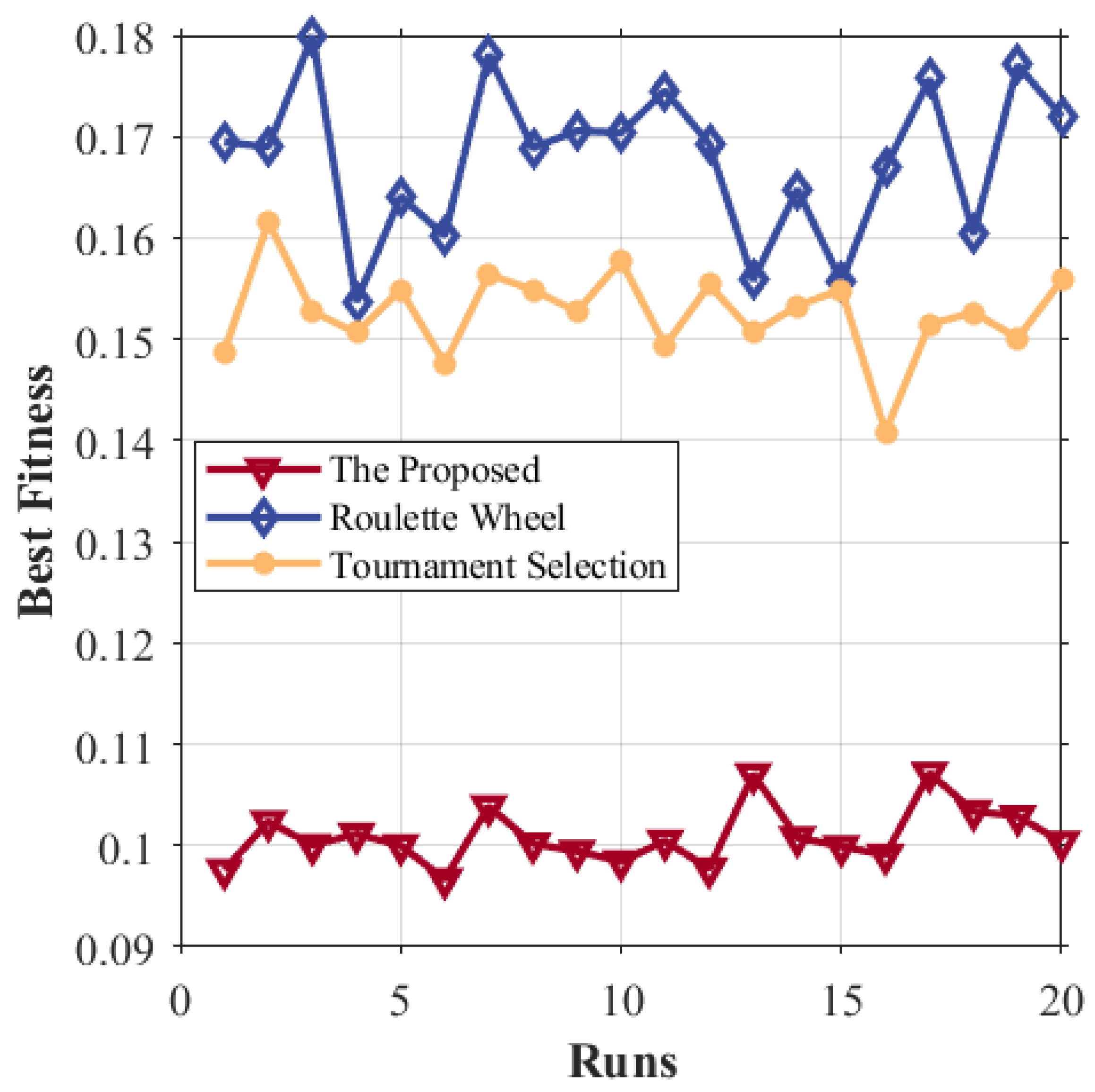
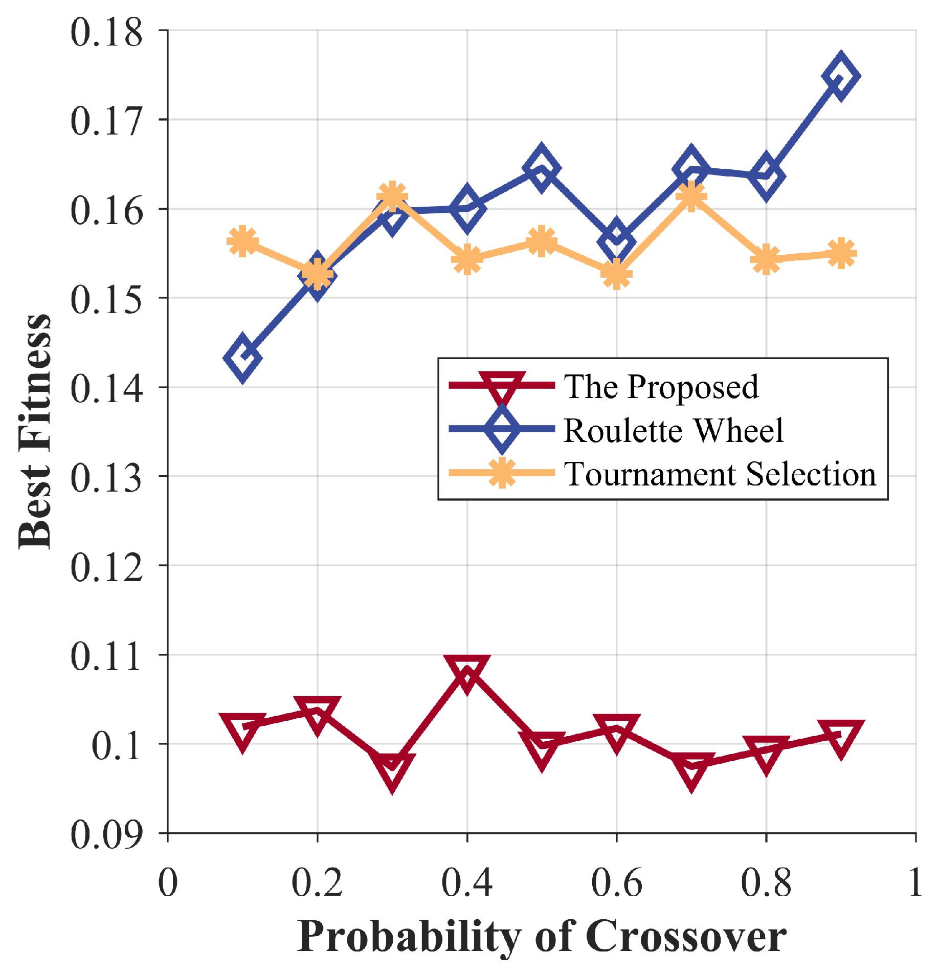
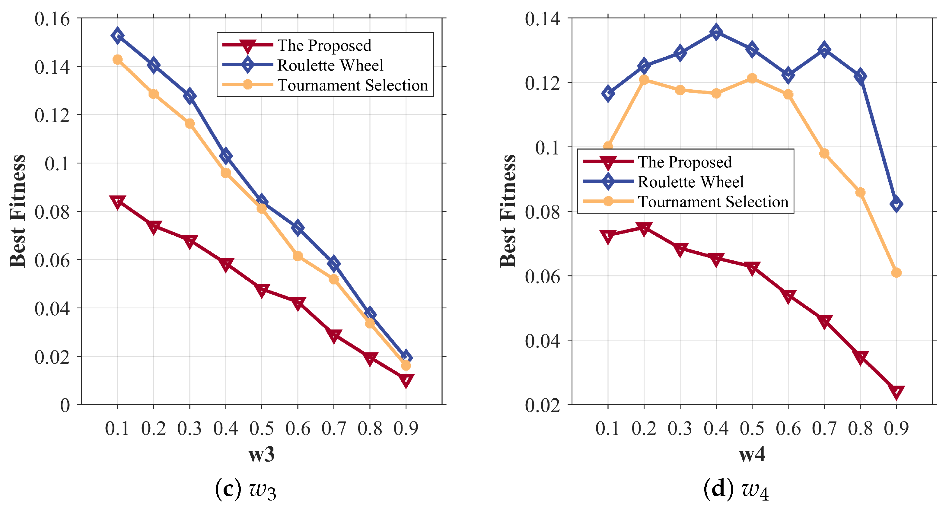
• Fuzzy-adaptive crossover strategy with dynamic parameter control: A fuzzy logic-guided crossover strategy was designed to autonomously adjust crossover patterns and intensities during evolutionary processes. By monitoring real-time metrics (e.g., population diversity index and fitness variance), the strategy adaptively balances exploration and exploitation, aggressively exploring new solutions in low-diversity scenarios while refining high-quality candidates in convergent phases. The experimental results demonstrate that this approach achieves a 40.47% improvement in average fitness over roulette wheel selection and 35.48% over tournament selection, with enhanced robustness across parameter variations.

1.4. Organization

The rest of this article is organized as follows. In Section 2, we concentrate on elucidating the problem model, the optimization goals, and the decision variables. In Section 3, we present the proposed scheme in detail. In Section 4, the corresponding simulation results are presented. Finally, Section 5 concludes this article.

2. Problem Formulation

The design of large-scale SAR constellations requires a rigorous mathematical framework to balance competing objectives such as revisit period, payload capability, cost, and coverage. This section establishes a multi-objective optimization model by defining quantitative metrics for each goal, formulating their corresponding objective functions, and integrating them into a unified framework through normalization and weighting. The decision variables—including orbital parameters (e.g., inclination and altitude) and payload specifications (e.g., quality factor)—are systematically analyzed to ensure compatibility with the proposed hybrid optimization algorithm.

2.1. Optimization Goals

The design of large-scale SAR constellations requires balancing multiple conflicting objectives to achieve optimal performance. This section formulates the optimization framework, integrating revisiting period, payload capability, cost efficiency, and global coverage into a unified objective function. The goals are quantified through rigorous mathematical modeling, ensuring compatibility with multi-objective optimization algorithms while addressing the inherent trade-offs between system performance and resource constraints.

2.1.1. Revisiting the Period Objective Function

The revisiting period $T_r$ is defined as the time interval required for a satellite to revisit a specific ground location. To minimize $T_r$, the objective function is formulated as the average revisiting period over the target region:

$$f_1=T_r$$

(1)

The specific calculation methods are as follows:

(1) Meshing

Assume that the range of the observation area in the longitude direction is $[{\lambda }_{min},{\lambda }_{max}]$, and in the latitude direction, it is $[{\phi }_{min},{\phi }_{max}]$. Here, we define the grid width w, which allows us to calculate the number of grids $N_{\lambda }$ in the longitude direction and $N_{\phi }$ in the latitude direction.

The number of grids in the longitude direction $N_{\lambda }$:

$$N_{\lambda }=⌈{\displaystyle \frac{{\lambda }_{\max }-{\lambda }_{\min }}{w}}⌉$$

(2)

The number of grids in the latitude direction $N_{\phi }$:

$$N_{\phi }=⌈{\displaystyle \frac{{\phi }_{\max }-{\phi }_{\min }}{w}}⌉$$

(3)

Thus, the entire observation area is divided into $N=N_{\lambda }\times N_{\phi }$ grids. Each grid can be represented by its central latitude and longitude coordinates $({\lambda }_i,{\phi }_j)$, where $i=1,2,\dots ,N_{\lambda }$ and $j=1,2,\dots ,N_{\phi }$.

(2) Calculation of Earth-fixed coordinates for satellites and target grids

The orbit of a satellite can be described using Keplerian orbital elements, which include orbital height h, eccentricity e, inclination i, right ascension of the ascending node $\Omega$, argument of periapsis $\omega$, and true anomaly f. Using relevant theories of orbital dynamics, it is possible to calculate the position coordinates of the satellite in the Earth-fixed coordinate system $(X_e\left(t\right),Y_e\left(t\right),Z_e\left(t\right))$.

For the target grid region, the latitude and longitude coordinates of the targets can be converted into Earth-fixed coordinates. This facilitates subsequent calculations of relative geometric relationships.

(3) Calculation of SAR satellite slant range visibility and incidence angle range

Given that the direction installation angle of the satellite antenna is ${\theta }_{ant}$, the visible viewing angle range can be defined as $\left[\max \left(10,{\theta }_{ant}-{\displaystyle \frac{\Theta }{2}}\right),\min \left({\theta }_{ant}+{\displaystyle \frac{\Theta }{2}},60\right)\right]$. Let the lower limit be ${\theta }_{min}$, and let the upper limit be ${\theta }_{max}$, i.e.,

$${\theta }_{min}=\max \left(10,{\theta }_{ant}-{\displaystyle \frac{\Theta }{2}}\right)$$

(4)

$${\theta }_{max}=\min \left({\theta }_{ant}+{\displaystyle \frac{\Theta }{2}},60\right)$$

(5)

Furthermore, based on the geometric relationship, the incident angles corresponding to the near end and far end can be calculated as follows:

$${\theta }_{i_{\min }}=\arcsin \left(\sin \left(90-{\theta }_{min}\right){\displaystyle \frac{R_e+h}{R_z}}\right)$$

(6)

$${\theta }_{i_{\max }}=\arcsin \left(\sin \left(90-{\theta }_{max}\right){\displaystyle \frac{R_e+h}{R_z}}\right)$$

(7)

(4) Calculating time series

Based on the working mode of the SAR and the geometric relationship, a grid can be observed by the SAR satellite if it satisfies the following two conditions simultaneously:

The center of the grid needs to be within the slant range visibility of the satellite, i.e.,

$${\theta }_{i_{\min }}\le {\theta }_i\left(t\right)\le {\theta }_{i_{\max }}$$

(8)

where ${\theta }_i\left(t\right)$ is the incidence angle of the grid center relative to the satellite at time t. The incidence angle ${\theta }_i\left(t\right)$ can be calculated using the position vectors of the center point and the satellite. Let the position vector of the satellite at time t be ${\overrightarrow{r}}_s\left(t\right)$, the velocity vector be ${\overrightarrow{v}}_s\left(t\right)$, and the position vector of the grid center be ${\overrightarrow{r}}_g$. The normal vector perpendicular to the ground at the target location is $\overrightarrow{n}={\displaystyle \frac{{\overrightarrow{r}}_g}{|{\overrightarrow{r}}_g|}}$, and the slant range vector between the target and the satellite is $\overrightarrow{s}\left(t\right)={\overrightarrow{r}}_s\left(t\right)-{\overrightarrow{r}}_g$. Then, the incidence angle is given by

$${\theta }_i\left(t\right)=\arccos \left({\displaystyle \frac{\overrightarrow{n}·\overrightarrow{s}}{|\overrightarrow{n}\left|\right|\overrightarrow{s}|}}\right)$$

(9)

The target azimuth angle needs to be within the SAR satellite’s azimuth scan range, i.e.,

$$\left|\gamma \left(t\right)\right|\le |{\theta }_{az{i}_{scan}}|$$

(10)

where $\gamma \left(t\right)$ represents the azimuth angle between the satellite and the target, and ${\theta }_{az{i}_{scan}}$ is generally the SAR satellite’s azimuth scanning capability. Let the vector between the satellite and the target be $\overrightarrow{d}\left(t\right)={\overrightarrow{r}}_g-{\overrightarrow{r}}_s\left(t\right)$. The angle between the vector from the satellite to the target and the satellite velocity vector is given by

$$\cos \beta \left(t\right)={\displaystyle \frac{\overrightarrow{d}·{\overrightarrow{v}}_s\left(t\right)}{|\overrightarrow{d}\left|\right|{\overrightarrow{v}}_s\left(t\right)|}}$$

(11)

The azimuth angle is then

$$\gamma \left(t\right)={90}^{\circ }-\beta \left(t\right)$$

(12)

Starting from the initial time $t_0$, advance the time using a time step $\Delta t$. For each grid $({\lambda }_i,{\phi }_j)$ and every satellite k in the constellation, check if both the incidence angle condition and the azimuth angle condition are simultaneously satisfied. If the conditions are met, record the time $t_m$ to form the time sequence $\{t_1,t_2,\cdots ,t_n\}$ for that grid.

(5) Calculating the revisit period metric

For each grid $({\lambda }_i,{\phi }_j)$, its time sequence is $\{t_1,t_2,\cdots ,t_n\}$. The revisit period sequence of the grid is $\{T_1=t_2-t_1,T_2=t_3-t_2,\cdots ,T_{n-1}=t_n-t_{n-1}\}$. The maximum revisit period of the grid is $T_{\max }^{ij}=\max \{T_1,T_2,\cdots ,T_{n-1}\}$. The average revisit period of the grid is $T_{\mathrm{ave}}^{ij}=\mathrm{mean}\{T_1,T_2,\cdots ,T_{n-1}\}$. The minimum revisit period of the grid is $T_{\min }^{ij}=\min \{T_1,T_2,\cdots ,T_{n-1}\}$.

By integrating the indicators of all grids, we can obtain the overall revisit period indicator for the entire region. Here, we use the method of averaging to obtain a single average indicator, which can accommodate all regional grids.

The average revisit period of the region is $T_r={\displaystyle \frac{1}{N}}{\sum }_{i=1}^{N_{\lambda }}{\sum }_{j=1}^{N_{\phi }}{T}_{\mathrm{ave}}^{ij}.$

2.1.2. SAR System Payload Capability Objective Function

The SAR payload system’s capability directly determines the system’s operational effectiveness, which is primarily influenced by resolution, swath width, and field of view (FOV). Drawing on engineering design experience, the payload capability is quantified by the quality factor (swath width divided by resolution) and the operational swath width. To unify the optimization direction (minimizing the objective function), the payload performance objective function is defined as the reciprocal of the product of the quality factor Q and the operational swath width $W_{width}$. A larger product $Q\times W_{width}$ indicates stronger payload capability, while the objective function’s inverse ensures alignment with minimization:

$$f_2={\displaystyle \frac{1}{Q\times W_{width}}}$$

(13)

where $Q={\displaystyle \frac{\mathrm{Swath}\mathrm{Width}\left(\mathrm{km}\right)}{\mathrm{Resolution}\left(\mathrm{m}\right)}}$ [27], representing the trade-off between spatial coverage and imaging precision. $W_{width}$ denotes the SAR system’s operational swath width.

The capability function for the SAR constellation is given by

$$P=\sum _{n=1}^{N}Q\left(n\right)·W_{width}\left(n\right)$$

(14)

where N represents the number of satellites, and $Q\left(n\right)$ and $W_{width}\left(n\right)$ represent the quality factor and visible width of the n-th satellite, respectively. According to the geometry, the calculation formula for $W_{width}\left(n\right)$ is as follows:

$$W_{width}\left(n\right)=\left[{\alpha }_{\max }\left(n\right)-{\alpha }_{\min }\left(n\right)\right]·Re$$

(15)

$${\alpha }_{\max }\left(n\right)=\left[\arcsin \left(\sin \left({\theta }_{\max }\left(n\right)\right)·{\displaystyle \frac{Re+h\left(n\right)}{Re}}\right)-{\theta }_{\max }\left(n\right)\right]$$

(16)

$${\alpha }_{\min }\left(n\right)=\left[\arcsin \left(\sin \left({\theta }_{\min }\left(n\right)\right)·{\displaystyle \frac{Re+h\left(n\right)}{Re}}\right)-{\theta }_{\min }\left(n\right)\right]$$

(17)

where ${\theta }_{\max }\left(n\right)$, ${\theta }_{\min }\left(n\right)$, and $h\left(n\right)$ represent the maximum viewing angle, minimum viewing angle, and orbital height of the n-th satellite, respectively, and $Re$ denotes the Earth’s radius at the subsatellite point.

2.1.3. Cost Objective Function

The cost mainly considers the hardware cost of the satellite. Let C be the total cost of the satellite constellation, and the cost objective function can be defined as

$$f_3=C$$

(18)

According to the SAR radar equation, the higher the satellite altitude (if the final image quality is to be maintained), the larger the required SAR power aperture product will be. The increased cost factors are mainly reflected in a larger antenna area and greater antenna power. The larger the SAR payload’s visible range $\Delta \theta$, the greater the antenna scanning capability needs to be, requiring more T/R component channels, thereby increasing the system antenna cost. Therefore, in the optimization design of SAR constellations, it is necessary to reasonably select the values of orbit height h, quality factor Q, and visible range $\theta$ under the premise of meeting task performance requirements to control the cost budget range. The cost calculation function for a SAR constellation is defined as follows:

$$C=\sum _{n=1}^N\left\{C_0+\left[c_{(Q,h)}\times f_{(Q,h)}(Q\left(n\right),h\left(n\right))+c_{\theta }\times f_{\left({\theta }_{scan}\right)}\left({\theta }_{scan}\left(n\right)\right)\right]\right\}$$

(19)

where $C_0$ is the fixed cost of the SAR system, and $c_{(Q,h)}$ is the hardware cost coefficient related to changes in the quality factor and orbit height. Based on engineering experience, this part accounts for 70–80% of the system cost, so $c_{(Q,h)}$ is generally taken as 0.7–0.8. $f_{(Q,h)}(Q\left(n\right),h\left(n\right))$ is a variation function related to the quality factor and orbit height, $c_{\theta }$ is the hardware cost coefficient related to the load scanning angle. According to the analysis of data from multiple SAR engineering projects, $c_{\theta }$ is generally taken between 0.3–0.4, and $f_{\left({\theta }_{scan}\right)}\left({\theta }_{scan}\left(n\right)\right)$ is a coefficient related to the load antenna scanning capability.

For ease of subsequent optimization analysis and calculations, we can define

$$f_{(Q,h)}(Q_{\min },h_{\min })=1$$

(20)

$$f_{\left({\theta }_{scan}\right)}\left({\theta }_{scan\min }\right)=1$$

(21)

In the case of fixed resolution, the quality factor is mainly related to the swath width and can be defined as

$$f(Q,h)=f(Q_0,h_0)\times \sqrt{{\displaystyle \frac{Q}{Q_{\min }}}}\times {\left({\displaystyle \frac{h}{h_{\min }}}\right)}^3$$

(22)

The function $f_{\left({\theta }_{\mathrm{scan}}\right)}\left({\theta }_{\mathrm{scan}}\left(n\right)\right)$ is primarily related to the scanning angle of the SAR antenna. The larger the scanning angle, the larger the required TR component scale, and thus the higher the antenna cost. Under a fixed grating lobe level, the inter-element spacing of the antenna can be calculated for any scanning angle, which in turn allows us to calculate the number of antenna channels, leading to $f_{\left({\theta }_{\mathrm{scan}}\right)}\left({\theta }_{\mathrm{scan}}\left(n\right)\right)$. By taking X-band SAR antennas as an example, this function is shown as follows:

$$f=\left\{\begin{array}{cc}1,\hfill & {\theta }_{\mathrm{scan}}\left(n\right)<1^{\circ }\hfill \\ [3.1·\exp (-1.8·{\theta }_{\mathrm{scan}}\left(n\right))+1.1·\exp (-0.3·{\theta }_{\mathrm{scan}}\left(n\right))]/16,\hfill & 1\le {\theta }_{\mathrm{scan}}\left(n\right)\le 3^{\circ }\hfill \\ [3.2·\exp (-0.9·\left({\theta }_{\mathrm{scan}}\left(n\right)\right))+1.1·\exp (-0.1·{\theta }_{\mathrm{scan}}\left(n\right))]/8,\hfill & 3^{\circ }<{\theta }_{\mathrm{scan}}\left(n\right))\le 5^{\circ }\hfill \\ [3.2·\exp (-0.4·\left({\theta }_{\mathrm{scan}}\left(n\right)\right))+1·\exp (-0.07·{\theta }_{\mathrm{scan}}\left(n\right))]/4,\hfill & 5^{\circ }<{\theta }_{\mathrm{scan}}\left(n\right)\le {10}^{\circ }\hfill \\ [3.1·\exp (-0.2·\left({\theta }_{\mathrm{scan}}\left(n\right)\right))+0.8·\exp (-0.02·{\theta }_{\mathrm{scan}}\left(n\right))]/2,\hfill & {10}^{\circ }<{\theta }_{\mathrm{scan}}\left(n\right)\le {20}^{\circ }\hfill \\ (1+\sin \left({\theta }_{\mathrm{scan}}\left(n\right)\right)),\hfill & {\theta }_{\mathrm{scan}}\left(n\right)>{20}^{\circ }\hfill \end{array}\right.$$

(23)

2.1.4. Coverage Function

For the coverage area, we typically hope that the satellite constellation can cover as much of the region as possible, meaning that the larger the coverage area, the better. To align with the unified optimization direction (minimizing the objective function value), we can define the objective function as the reciprocal of the coverage area.

Let A be the coverage area of the satellite constellation over a region of the Earth. Then, the coverage area objective function is

$$f_3={\displaystyle \frac{1}{A}}$$

(24)

According to the satellite orbit parameters, by using Kepler’s laws and coordinate transformation formulas, we can obtain the position vector of the satellite in the spatial Cartesian coordinate system ${\overrightarrow{r}}_s=(x_s,y_s,z_s)$.

Let the intersection point of the SAR system’s maximum viewing angle ${\theta }_{\max }$ with the Earth’s surface be $P(x_p,y_p,z_p)$. Then, the vector $\overrightarrow{SP}$ is

$$\overrightarrow{SP}={\overrightarrow{r}}_p-{\overrightarrow{r}}_s$$

(25)

where ${\overrightarrow{r}}_p$ is the position vector of the intersection point P. Here, we also need to consider the constraint condition that the vector between the satellite and the target is perpendicular to the satellite velocity vector. According to the dot product formula and the ellipsoid equation, we can obtain

$$\left\{\begin{array}{c}\overrightarrow{SP}·{\overrightarrow{v}}_s=|\overrightarrow{SP}\left|\right|{\overrightarrow{v}}_s|\cos {\theta }_{\max }\hfill \\ \overrightarrow{SP}·{\overrightarrow{n}}_s=0\hfill \\ {\displaystyle \frac{x_p^2}{a^2}}+{\displaystyle \frac{y_p^2}{a^2}}+{\displaystyle \frac{z_p^2}{b^2}}=1\hfill \end{array}\right.$$

(26)

where a is the Earth’s semi-major axis, and b is the Earth’s semi-minor axis.

Combining the above vector relationships and the ellipsoid equation, the latitude ${\phi }_p$ of the intersection point P can be calculated from its position vector $(x_p,y_p,z_p)$:

$$\tan \phi ={\displaystyle \frac{z_p}{\sqrt{x_p^2+y_p^2}}}$$

(27)

Iterate through all satellites in the constellation, recording the latitude range covered by each satellite $\left([{\phi }_{min}^s,{\phi }_{max}^s]\right)$. Find the minimum value of all satellite coverage latitude ranges as the southernmost latitude of the constellation’s coverage (${\phi }_{min}^{constellation}={\min }_{s=1}^n{\phi }_{min}^s$) and the maximum value as the northernmost latitude of the constellation’s coverage (${\phi }_{max}^{constellation}={\max }_{s=1}^n{\phi }_{max}^s$).

To calculate the surface area for a specific latitude interval on an ellipsoid like Earth, which is relatively complex, numerical integration methods can be used. For a point on the Earth’s surface with latitude $\phi$ and longitude $\lambda$, the infinitesimal area $dS$ at that point in the ellipsoidal coordinate system can be expressed as

$$dS=a\cos \phi \sqrt{1-e^2{\sin }^2\phi }d\lambda d\phi$$

(28)

where $(e=\sqrt{1-{\displaystyle \frac{b^2}{a^2}}})$ is the Earth’s eccentricity. By performing a double integral on the infinitesimal area within the longitude range $[0,2\pi ]$ and the latitude range $[{\phi }_{min}^{constellation},{\phi }_{max}^{constellation}]$, we can obtain the maximum ground area covered by the constellation:

$$A_{\max }=2\pi I_{\phi }$$

(29)

2.1.5. Establishing a Comprehensive Objective Function

The optimization design of a SAR constellation is a multi-objective optimization problem. Therefore, it is necessary to assign appropriate weights to each objective based on specific task requirements and practical conditions. The four objective functions are combined into a comprehensive objective function F using the weighted sum method:

$$F={\omega }_1{f}_1+{\omega }_2{f}_2+{\omega }_3{f}_3+{\omega }_4{f}_4$$

(30)

where ${\omega }_i$ represents the weight assigned to the i-th objective function $f_i$. The weights must satisfy the following constraints:

$${\omega }_1+{\omega }_2+{\omega }_3+{\omega }_4=1,0\le {\omega }_i\le 1,i=1,2,3,4$$

(31)

2.2. Decision Variables

Decision variables are parameters that can directly affect the performance of a SAR constellation and are closely related to the optimization objectives. The main decision variables include orbital parameters and satellite system parameters. These variables each have their specific value ranges, which are determined based on engineering considerations, satellite technical limitations, and mission requirements. The

Table 1. Definition and range of decision variables.

Decision Variable	Symbol	Value Range
Number of Satellites	N	$N\in {\mathbb{Z}}^{+}$
Satellite Altitude	h	[400, 1000] km
Orbital Inclination	i	[0°, 180°]
Right Ascension of Ascending Node	$\Omega$	[0°, 360°)
Argument of Perigee	M	[0°, 360°)
Field of View	${\theta }_s$	[3°, 60°]
Quality Factor	Q	[10, 100]

presents the value ranges of decision variables adopted for subsequent optimization.

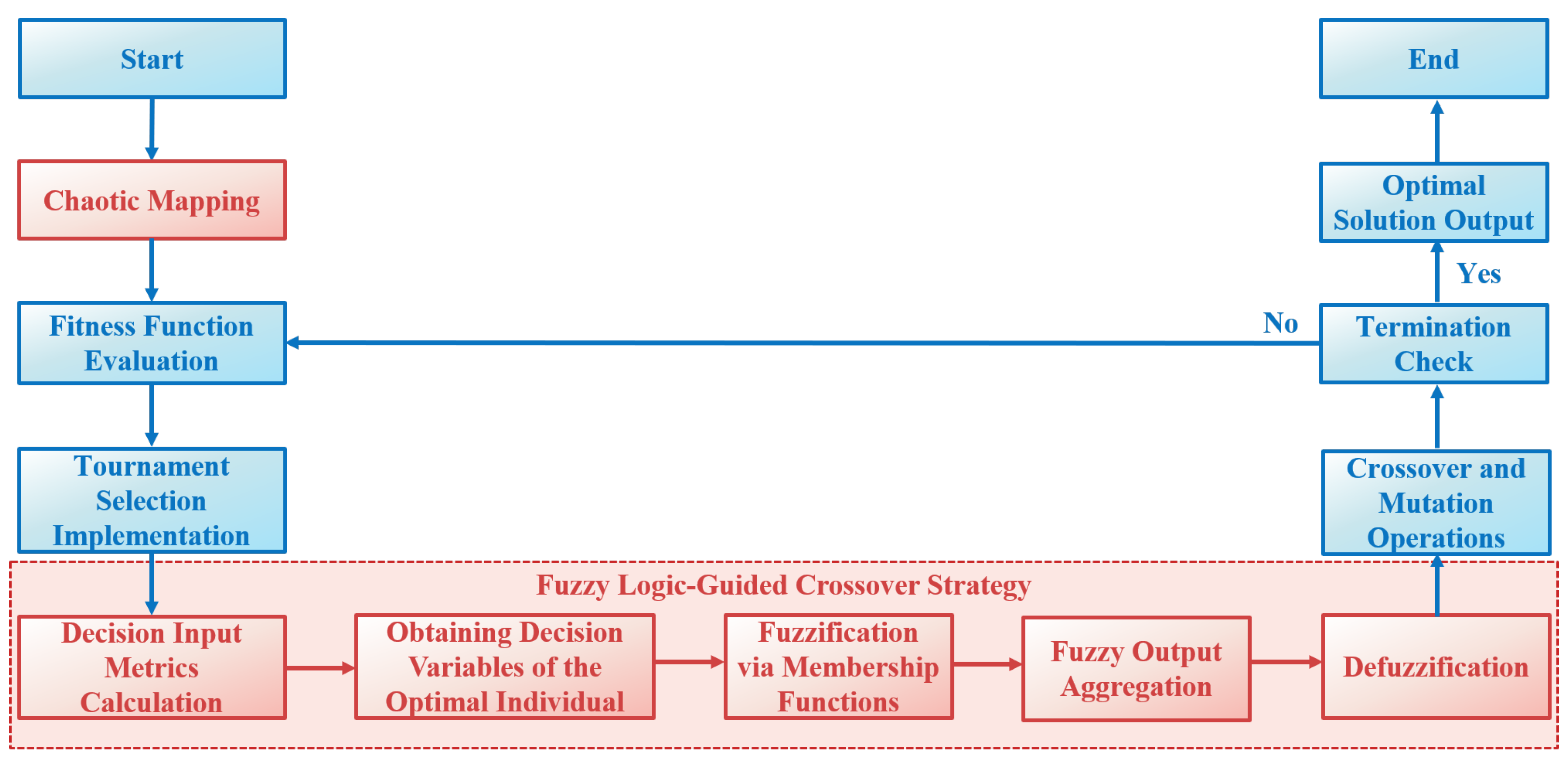
3. The Proposed Method

In this section, we present a novel hybrid optimization framework that synergistically integrates chaotic sequence initialization and fuzzy rule-based decision-making for the orbital design optimization of large-scale SAR constellations. The proposed methodology addresses the high-dimensional challenge inherent in constellation design by combining the global exploration capability of chaotic sequences with the adaptive control mechanism of fuzzy logic systems. The algorithm workflow consists of six primary components, as illustrated in Figure 2, which are elaborated as follows:

3.1. Step 1: Initial Population Generation via Chaotic Mapping

In the optimization of SAR constellations, designing and analyzing the initial population is crucial to avoid local optima. This paper primarily employs a generation method based on chaotic mapping, specifically introducing a Logistic map to enhance the diversity of the initial population. During the generation process, the characteristics of chaotic sequences are utilized to generate chaotic values for each satellite or decision variable. This ensures that the initial population is more randomly and ergodically distributed in the solution space, increasing the likelihood of finding the global optimum.

The calculation formula for the Logistic map is given by

$$x_{n+1}=\mu x_n(1-x_n)$$

(32)

where $x_n\in (0,1)$ is the chaotic variable, and $\mu$ is the control parameter. When $\mu =4$, the Logistic map is in a state of complete chaos.

Taking the satellite orbital height h as an example, its value range $[h_{min},h_{max}]$ can be transformed using the above equation:

$$h_n=h_{min}+(h_{max}-h_{min})·x_n$$

(33)

Similarly, this method can be applied to other decision variables to generate their values, thereby creating an initial population that includes all decision variables.

3.2. Step 2: Fitness Evaluation for All Individuals in the Population

The fitness of each individual in the population is calculated to assess its quality and suitability as a potential solution. The fitness function is designed to incorporate multiple performance metrics relevant to SAR constellation optimization.

3.3. Step 3: Tournament Selection Based on Fitness Evaluation Results

To ensure the selection of high-quality individuals while maintaining population diversity, a tournament selection mechanism is employed. This method probabilistically selects superior individuals by comparing randomly sampled subsets of the population based on their fitness rankings.

(1) Roulette wheel selection [28,29] combined with elitism preservation [30]

Assume the population $P=\{x_1,x_2,\dots ,x_N\}$ contains N individuals, where the fitness of each individual $x_i$ is denoted as $f\left(x_i\right)$. The total fitness of the population can be expressed as

$$F=\sum _{i=1}^{N}f\left(x_i\right)$$

(34)

In roulette wheel selection, the probability $p\left(x_i\right)$ that an individual $x_i$ is selected is calculated using the following formula:

$$p\left(x_i\right)={\displaystyle \frac{f\left(x_i\right)}{F}},i=1,2,\dots ,N$$

(35)

To implement the selection process, we typically compute the cumulative probability $q\left(x_i\right)$, which is given by

$$q\left(x_i\right)=\sum _{j=1}^{i}p\left(x_j\right),i=1,2,\dots ,N$$

(36)

During the selection phase, a random number r within the interval $[0,1]$ is generated. If $q\left(x_{k-1}\right)<r\le q\left(x_k\right)$, then the individual $x_k$ is selected.

The elitism preservation strategy involves directly retaining the top m ($m<N$) individuals with the highest fitness values in the next generation without participating in the aforementioned roulette wheel selection process.

(2) Tournament selection [31,32] combined with elitism preservation

In tournament selection, at each step, k individuals are randomly selected from the population P to form a tournament subset $T=\{x_{i_1},x_{i_2},\dots ,x_{i_k}\}$. The fitness values of these k individuals are compared, and the individual with the highest fitness, denoted as $x_{best}=\arg {\max }_{j=1}^{k}f\left(x_{i_j}\right)$, is chosen to proceed to the next generation. This process is repeated $N-m$ times (where m is the number of elite individuals), and the selected individuals are combined with the m elite individuals to form the next generation population.

Assume the population contains N individuals with fitness values $\{f_1,f_2,\cdots ,f_N\}$. In a single tournament selection, t individuals are randomly chosen, with their fitness values being $\{f_{i_1},f_{i_2},\cdots ,f_{i_t}\}$. The probability that an individual j wins in this tournament (i.e., is selected) can be calculated as follows:

Let $\mathcal{F}$ be the set of all possible tournament groups. For a specific tournament group $S\in \mathcal{F}$ that includes individual j, the probability that individual j wins within this group is

$$P\left(j\right|S)=\prod _{k\ne j,k\in S}I(f_j>f_k)$$

(37)

Here, $I(·)$ is the indicator function, which takes the value 1 if the condition inside the parentheses is true; it takes 0 otherwise. The probability that individual j wins across all possible tournament groups, denoted as $P\left(j\right)$, is given by

$$P\left(j\right)={\displaystyle \frac{1}{C_{N-1}^{t-1}}}\sum _{S\in \mathcal{F},j\in S}\prod _{k\ne j,k\in S}I(f_j>f_k)$$

(38)

Here, $C_n^m={\displaystyle \frac{n!}{m!(n-m)!}}$ represents the binomial coefficient, which indicates the number of ways to choose m elements from a set of n elements.

While roulette wheel selection combined with elitism offers simplicity and effective utilization of fitness information in scenarios with accurate fitness evaluation and low computational complexity demands, it suffers from premature convergence and high sensitivity to fitness scaling. These limitations make it less suitable for complex multi-objective optimization problems like SAR constellation design, where local optima trapping is a critical concern.

In contrast, tournament selection with elitism demonstrates superior performance:

• It mitigates premature convergence through stochastic selection pressure;
• It reduces sensitivity to fitness value variations by comparing local subsets;
• It balances exploitation and exploration more effectively in high-dimensional search spaces.

These characteristics make tournament selection with elitism particularly advantageous for complex optimization problems requiring extensive solution space exploration. Consequently, this strategy is adopted in our framework to address the multi-modal challenges inherent in SAR constellation design.

3.4. Step 4: Fuzzy Logic-Guided Crossover Strategy

In the crossover operation, we propose a fuzzy rule-based crossover mechanism tailored to the optimization characteristics of spaceborne SAR constellations. Fuzzy theory, with its unique capability to handle uncertainty and imprecise information, is integrated into the crossover process to enable the adaptive adjustment of crossover patterns and intensities based on problem-specific features and requirements. This approach allows the algorithm to strike an optimal balance between exploring novel solutions and exploiting existing knowledge. The fuzzy logic-guided [33,34] crossover process consists of the following sub-steps:

3.4.1. Decision Input Metrics Calculation

Three critical indicators are computed for the current population:

• Population diversity (D): This is measured using the average Euclidean distance between individuals in the solution space;
• Fitness gap (G): Defined as the difference between the maximum and median fitness values in the population;
• Convergence speed (V): Calculated as the slope of the best fitness curve over the last $\Delta t$ generations.

3.4.2. Obtaining Decision Variables of the Current Optimal Individual

After each generation of population evolution, the decision variables of the superior individuals in the new population will be used as inputs for fuzzy decision-making. These variables as shown in

Table 2. Decision variables for fuzzy decision input.

Decision Variable	Symbol	Value Range
Satellite Altitude	h	$[h_{min},h_{max}]$ km
Orbital Inclination	i	$0^{\circ }$ to ${180}^{\circ }$
Right Ascension of the Ascending Node	$\Omega$	$[0^{\circ },{360}^{\circ })$
Argument of Perigee	$\omega$	$[0^{\circ },{360}^{\circ })$
True Anomaly	M	$[0^{\circ },{360}^{\circ })$
Visible Range	$\theta$	$[2^{\circ },{50}^{\circ }]$
Quality Factor	Q	$[10,100]$

mainly include the following:

3.4.3. The Input Variables Are Fuzzified Using Predefined Membership Functions

To illustrate the application of fuzzy rules, we consider population diversity and satellite altitude. The fuzzy sets for population diversity are defined as “Low”, “Medium”, and “High”.

-

Low: Indicates high similarity among individuals in the population, implying insufficient diversity;

-

Medium: Indicates that diversity is at a moderate level;

-

High: Indicates significant differences among individuals, implying rich diversity.

The membership function used is a trapezoidal membership function. Let D be the population diversity index, with $D_{\min }$ and $D_{\max }$ representing the minimum and maximum values of population diversity, respectively.

For low diversity, the membership function ${\mu }_{low}\left(D\right)$ is determined by four parameters: $a_1$, $b_1$, $c_1$, and $d_1$:

$${\mu }_{low}\left(D\right)=\left\{\begin{array}{cc}0,\hfill & D\le a_1\mathrm{or}D\ge d_1\hfill \\ {\displaystyle \frac{D-a_1}{b_1-a_1}},\hfill & a_1<D\le b_1\hfill \\ 1,\hfill & b_1<D\le c_1\hfill \\ {\displaystyle \frac{d_1-D}{d_1-c_1}},\hfill & c_1<D\le d_1\hfill \end{array}\right.$$

(39)

Medium diversity is determined using four parameters: $a_2$, $b_2$, $c_2$, and $d_2$. The membership function ${\mu }_{medium}\left(D\right)$ is defined as

$${\mu }_{medium}\left(D\right)=\left\{\begin{array}{cc}0,\hfill & D\le a_2\mathrm{or}D\ge d_2\hfill \\ {\displaystyle \frac{D-a_2}{b_2-a_2}},\hfill & a_2<D\le b_2\hfill \\ 1,\hfill & b_2<D\le c_2\hfill \\ {\displaystyle \frac{d_2-D}{d_2-c_2}},\hfill & c_2<D\le d_2\hfill \end{array}\right.$$

(40)

High diversity is determined using four parameters: $a_3$, $b_3$, $c_3$, and $d_3$. The membership function ${\mu }_{high}\left(D\right)$ is defined as

$${\mu }_{high}\left(D\right)=\left\{\begin{array}{cc}0,\hfill & D\le a_3\mathrm{or}D\ge d_3\hfill \\ {\displaystyle \frac{D-a_3}{b_3-a_3}},\hfill & a_3<D\le b_3\hfill \\ 1,\hfill & b_3<D\le c_3\hfill \\ {\displaystyle \frac{d_3-D}{d_3-c_3}},\hfill & c_3<D\le d_3\hfill \end{array}\right.$$

(41)

The fuzzy sets for satellite orbit altitude are defined as “Low Altitude”, “Medium Altitude”, and “High Altitude”.

-

Low Altitude: Favors low cost but has a small coverage area;

-

Medium Altitude: Balances cost and coverage area;

-

High Altitude: Has a large coverage area but is costly.

Trapezoidal membership functions are used. Let H be the orbit height, with $H_{\min }$ and $H_{\max }$ representing the minimum and maximum values of orbit height, respectively. For the trapezoidal membership functions corresponding to “Small”, “Medium”, and “Large” fitness gaps, the parameters are $\{a_1^{\prime },b_1^{\prime },c_1^{\prime },d_1^{\prime }\}$, $\{a_2^{\prime },b_2^{\prime },c_2^{\prime },d_2^{\prime }\}$, and $\{a_3^{\prime },b_3^{\prime },c_3^{\prime },d_3^{\prime }\}$, respectively. The membership functions are defined as follows:

$${\mu }_{low}\left(H\right)=\left\{\begin{array}{cc}0,\hfill & H\le a_1^{\prime }\mathrm{or}H\ge d_1^{\prime }\hfill \\ {\displaystyle \frac{H-a_1^{\prime }}{b_1^{\prime }-a_1^{\prime }}},\hfill & a_1^{\prime }<H\le b_1^{\prime }\hfill \\ 1,\hfill & b_1^{\prime }<H\le c_1^{\prime }\hfill \\ {\displaystyle \frac{d_1^{\prime }-H}{d_1^{\prime }-c_1^{\prime }}},\hfill & c_1^{\prime }<H\le d_1^{\prime }\hfill \end{array}\right.$$

(42)

$${\mu }_{middle}\left(H\right)=\left\{\begin{array}{cc}0,\hfill & H\le a_2^{\prime }\mathrm{or}H\ge d_2^{\prime }\hfill \\ {\displaystyle \frac{H-a_2^{\prime }}{b_2^{\prime }-a_2^{\prime }}},\hfill & a_2^{\prime }<H\le b_2^{\prime }\hfill \\ 1,\hfill & b_2^{\prime }<H\le c_2^{\prime }\hfill \\ {\displaystyle \frac{d_2^{\prime }-H}{d_2^{\prime }-c_2^{\prime }}},\hfill & c_2^{\prime }<H\le d_2^{\prime }\hfill \end{array}\right.$$

(43)

$${\mu }_{high}\left(H\right)=\left\{\begin{array}{cc}0,\hfill & H\le a_3^{\prime }\mathrm{or}H\ge d_3^{\prime }\hfill \\ {\displaystyle \frac{H-a_3^{\prime }}{b_3^{\prime }-a_3^{\prime }}},\hfill & a_3^{\prime }<H\le b_3^{\prime }\hfill \\ 1,\hfill & b_3^{\prime }<H\le c_3^{\prime }\hfill \\ {\displaystyle \frac{d_3^{\prime }-H}{d_3^{\prime }-c_3^{\prime }}},\hfill & c_3^{\prime }<H\le d_3^{\prime }\hfill \end{array}\right.$$

(44)

These trapezoidal membership functions map the crisp value of orbit height H into degrees of membership in the “Low Altitude”, “Medium Altitude”, and “High Altitude” fuzzy sets, respectively. These memberships can then be used in subsequent fuzzy inference processes to guide the optimization algorithm.

3.4.4. Incorporating Fuzzified Results into Relevant Fuzzy Rules

The fuzzy rule for crossover strategy selection probability based on population diversity and fitness gap is as shown in

Table 3. Fuzzy rules for crossover strategy selection based on population diversity and fitness gap.

Rule	Population Diversity	Fitness Gap	Single-Point Crossover	Multi-Point Crossover	Uniform Crossover
Rule 1	High	Large	Low	Medium	High
Rule 2	High	Medium	Medium	Medium	Medium
Rule 3	High	Small	Medium	High	Medium
Rule 4	Medium	Large	Medium	High	Medium
Rule 5	Medium	Medium	Medium	Medium	Medium
Rule 6	Medium	Small	Low	Medium	Medium
Rule 7	Low	High	Medium	Medium	Low
Rule 8	Low	Medium	Medium	Medium	Low
Rule 9	Low	Small	High	Low	Low

:

In SAR satellite optimization, fuzzy rules can be effectively formulated based on the weight values ${\omega }_1$ (revisit cycle), ${\omega }_2$ (SAR system performance), ${\omega }_3$ (coverage range), and ${\omega }_4$ (cost) to achieve multi-objective optimization. Specific considerations include the following:

When ${\omega }_1$ is large (emphasizing revisit cycle): If the current revisit cycle is “long”, the crossover position tends to lower the orbital altitude and increase the system’s field of view.

When ${\omega }_2$ is large (emphasizing SAR system performance): If the SAR system performance evaluation is “poor”, the crossover position tends to explore better values at the boundaries of key parameter variable regions for quality factors and viewing ranges.

When ${\omega }_3$ is large (emphasizing coverage range): If the current coverage range is “small”, the crossover position tends to enhance coverage within the satellite inclination variable region and increase the visible range within the SAR payload’s visible range variable region.

When ${\omega }_4$ is large (emphasizing cost): If the current cost is “high”, the crossover position tends to explore low-cost solutions within the orbital altitude, SAR payload quality factor, and SAR visible range variable regions.

In SAR satellite optimization, the crossover proportion rules can be formulated based on multiple factors, such as the evolutionary state of the population and the quality distribution of the current solutions. The following

Table 4. Fuzzy rules for crossover proportion.

Rule	Population Diversity	Fitness Gap	Crossover Proportion
Rule 1	Low	Small	Low (e.g., 0.2)
Rule 2	Low	Large	Medium (e.g., 0.5)
Rule 3	Low	Medium	Medium (e.g., 0.5)
Rule 4	Medium	Large	High (e.g., 0.7)
Rule 5	Medium	Medium	Medium (e.g., 0.5)
Rule 6	Medium	Small	Low (e.g., 0.3)
Rule 7	High	Large	High (e.g., 0.8)
Rule 8	High	Medium	Medium (e.g., 0.5)
Rule 9	High	Small	Medium (e.g., 0.5)

summarizes the fuzzy rules for determining the crossover proportion:

3.4.5. Aggregate Fuzzy Outputs

Matching rules: The fuzzified inputs are matched with the antecedent conditions of all fuzzy rules. For example, consider a rule stating, “If the population diversity is ‘High’ and the fitness gap is ‘Large’, then the single-point crossover probability is ‘Low’, the multi-point crossover probability is ‘Medium’, and the uniform crossover probability is ‘High’”. Check if the current input membership values satisfy these antecedent conditions.

Calculating activation strength: If the antecedent conditions of a rule are connected by an “AND” operation, the activation strength of the rule is typically taken as the minimum value of the membership degrees of these conditions. If they are connected by an “OR” operation, the maximum value is taken. For instance, in the aforementioned rule, if the membership degree for “High” population diversity is 0.8 and the membership degree for “Large” fitness gap is 0.7, the activation strength of the rule would be 0.8.

Based on the fuzzy rule base, each rule is matched. For example, for the rule “If the population diversity is ‘High’ and the fitness gap is ‘Large’, then the selection probability for uniform crossover is ‘High’”, calculate the membership degree of the antecedent conditions. Then, based on this membership degree, activate the conclusion part of the rule to obtain the fuzzy output indicating a “High” selection probability for uniform crossover.

The same process is applied to all rules to obtain the activation strengths of the output variables under different fuzzy sets. Aggregate the fuzzy outputs of all rules to obtain the overall fuzzy output for each output variable.

3.4.6. Defuzzification

First, after completing rule matching and inference, we obtain the fuzzy outputs corresponding to each rule. Each fuzzy output is typically a fuzzy set, and the defuzzification process converts these fuzzy outputs into crisp values using the centroid method. The principle of the centroid method is as follows:

Assume that the fuzzy set A has n elements $(x_1,x_2,\dots ,x_n)$, with corresponding membership degrees $({\mu }_1,{\mu }_2,\dots ,{\mu }_n)$. The centroid $C_A$ of this fuzzy set is calculated by

$$C_A={\displaystyle \frac{{\sum }_{i=1}^n{x}_i{\mu }_i}{{\sum }_{i=1}^n{\mu }_i}}$$

(45)

By calculating the centroid, the fuzzy outputs from various rules can be reasonably aggregated into a specific value, which can serve as the final decision or basis for further analysis. For example, for the fuzzy output of crossover strategy selection probability, calculate the centroid of the area under the membership function curve and use the corresponding numerical value as the final crossover strategy selection probability.

Through the defuzzification process, the overall fuzzy output of each output variable is converted into precise numerical values, such as specific crossover strategy selection probabilities, crossover position tendencies, and crossover ratios.

3.5. Step 5: Crossover and Mutation Operations

Based on the obtained crossover strategy selection probabilities, the specific crossover strategy for this operation is determined using a random selection method. For example, if the selection probabilities for single-point crossover, multi-point crossover, and uniform crossover are $P_1$, $P_2$, and $P_3$, respectively, a random number r between 0 and 1 can be generated. If $r<P_1$, then single-point crossover is selected; if $P_1\le r<P_1+P_2$, then multi-point crossover is chosen; if $r\ge P_1+P_2$, uniform crossover is selected.

According to the crossover position tendency values, each gene position is ranked, and those with higher tendency values are chosen as crossover positions. A threshold can be set to select gene positions with tendency values above this threshold; alternatively, the top k gene positions with the highest tendency values can be chosen.

Following the specified crossover ratio, the corresponding number of individuals are randomly selected from the population to participate in the crossover operation. For instance, if the crossover ratio is 0.8 and there are N individuals in the population, then $0.8\times N$ individuals are randomly selected for crossover.

Since the selection process has already produced better individuals according to the rules, the mutation probability should not be too high in this algorithm. Therefore, a mutation probability of 0.1 is adopted here.

3.6. Step 6: Termination Check

The termination condition is evaluated to determine whether the optimization process should conclude. Specifically, the algorithm checks if the current generation count t has reached the predefined maximum generation limit $T_{\max }$. If $t\ge T_{\max }$, the algorithm terminates and outputs the best individual (optimal solution) found during the evolutionary process. Otherwise, the process loops back to Step 2: Fitness evaluation for the next generation.

4. Simulation Results

To evaluate the effectiveness and robustness of the proposed processing framework and algorithm, we designed a simulated scenario for a case study. This section outlines the simulation process and presents the results achieved using the proposed method.

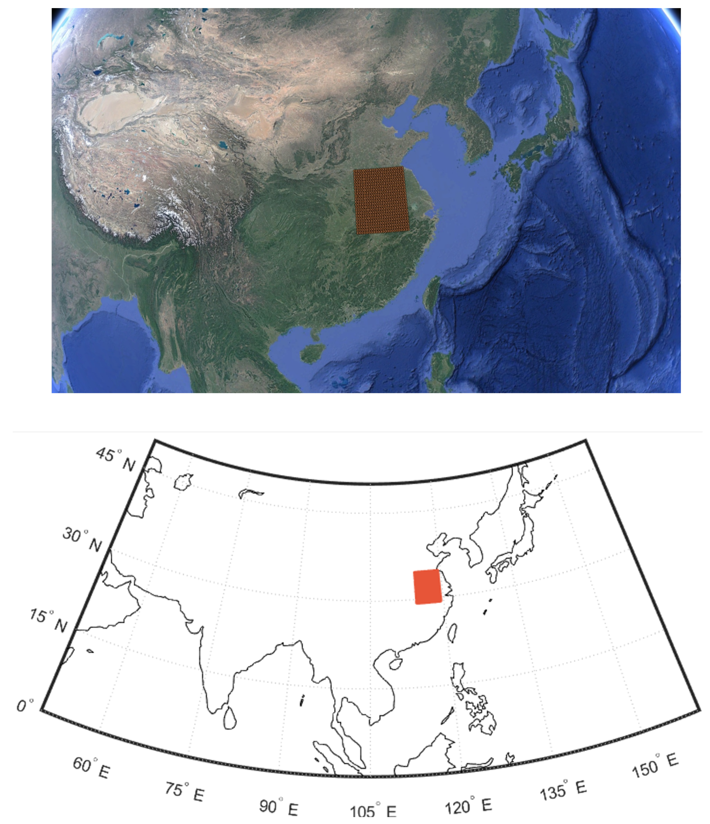
4.1. Simulation Settings

This study focuses on the orbital design of a 12-satellite constellation, where the revisit performance is evaluated over a geographic region in Anhui Province, China. The target area is bounded by a longitude ranging from 114.54° to 119.46° and a latitude ranging from 29.41° to 34.68°, as shown in Figure 3.

To validate the proposed algorithm, we compared it with two classical algorithms: roulette wheel selection and tournament selection.

In the Monte Carlo experiments, each of the three algorithms was tested across 20 independent runs. For the parameter sensitivity analysis, nine experiments were conducted for each of the key parameters: population size and crossover probability. In the robustness analysis, the weight parameters $w_1$, $w_2$, $w_3$, and $w_4$ were varied to evaluate their impact on algorithm performance.

4.2. Monte Carlo Experiment Results

The experimental comparison results of 20 runs with different algorithms are shown in Figure 4. The proposed method demonstrates superior performance compared to the roulette wheel and tournament selection methods. Specifically, the maximum best fitness achieved by the proposed method is approximately 0.11, which is significantly lower than the maximum values obtained by the roulette wheel (around 0.18) and tournament selection (around 0.16). The minimum best fitness for the proposed method is around 0.09, which outperforms the other two methods. The average best fitness across all runs for the proposed method is approximately 0.10, representing a substantial improvement over the roulette wheel (average around 0.168) and tournament selection (average around 0.155). This translates to an average improvement of about 40.47% and 35.48% over the roulette wheel and tournament selection methods, respectively. These results highlight the robustness and effectiveness of the proposed method in achieving higher-quality solutions consistently.

To further analyze the convergence speed, we present the results of a single experimental run over 5000 iterations, as shown in Figure 5. It is evident that the proposed algorithm exhibits faster convergence compared to both the roulette wheel and tournament selection methods. Specifically, the proposed method reaches a stable fitness value significantly earlier in the iterative process, demonstrating its ability to efficiently explore and exploit the search space. This accelerated convergence can be attributed to the integration of fuzzy logic-guided crossover and chaos-based initialization, which enhance both exploration and exploitation capabilities. These findings validate the effectiveness of the proposed approach in achieving superior performance while maintaining computational efficiency.

To further demonstrate the effectiveness of the proposed algorithm, we include practical optimization results by comparing the final satellite constellation configurations produced by the proposed algorithm with those generated by two commonly used baseline strategies: the roulette wheel and tournament selection algorithms.

The optimization results of different algorithms are shown in

Table 5. Optimization results of the roulette wheel algorithm.

Satellite No.	Orbit Altitude (km)	Inclination ${(}^{\circ })$	Ascending Node Longitude ${(}^{\circ })$	Argument of Perigee ${(}^{\circ })$	True Anomaly ${(}^{\circ })$	Quality Factor	Viewing Angle Range ${(}^{\circ })$
1	558.85	180.00	246.92	346.36	12.83	70.00	47.74
2	657.92	37.70	360.00	360.00	360.00	100.00	50.00
3	673.68	152.50	360.00	360.00	341.77	100.00	38.84
4	569.23	144.30	268.50	34.84	227.25	70.00	50.00
5	741.18	44.70	360.00	16.48	246.73	30.00	50.00
6	669.25	141.60	360.00	360.00	360.00	90.00	50.00
7	534.46	99.10	360.00	360.00	283.09	100.00	24.03
8	744.05	142.70	360.00	64.91	252.62	60.00	39.78
9	405.23	145.40	360.00	360.00	300.03	80.00	50.00
10	959.07	135.00	360.00	299.06	283.09	60.00	50.00
11	1000.00	134.50	360.00	290.66	354.61	100.00	50.00
12	606.55	142.10	305.23	360.00	268.08	50.00	44.76

,

Table 6. Optimization results of the tournament selection algorithm.

Satellite No.	Orbit Altitude (km)	Inclination ${(}^{\circ })$	Ascending Node Longitude ${(}^{\circ })$	Argument of Perigee ${(}^{\circ })$	True Anomaly ${(}^{\circ })$	Quality Factor	Viewing Angle Range ${(}^{\circ })$
1	814.08	136.30	360.00	360.00	60.13	10.00	50.00
2	648.43	34.10	360.00	360.00	360.00	10.00	50.00
3	623.78	39.00	360.00	317.73	360.00	10.00	50.00
4	576.40	151.20	360.00	357.23	360.00	50.00	50.00
5	833.44	39.50	17.31	360.00	360.00	10.00	50.00
6	1000.00	121.20	186.21	360.00	55.27	10.00	50.00
7	750.55	136.70	360.00	360.00	360.00	20.00	50.00
8	615.96	142.80	241.37	195.75	172.39	90.00	50.00
9	712.79	105.30	170.38	349.33	313.59	60.00	50.00
10	804.32	142.70	360.00	254.92	360.00	100.00	47.20
11	972.87	26.50	133.37	37.35	295.58	10.00	50.00
12	890.54	31.40	317.98	171.10	118.82	70.00	50.00

and

Table 7. Optimization results of the proposed algorithm.

Satellite No.	Orbit Altitude (km)	Inclination ${(}^{\circ })$	Ascending Node Longitude ${(}^{\circ })$	Argument of Perigee ${(}^{\circ })$	True Anomaly ${(}^{\circ })$	Quality Factor	Viewing Angle Range ${(}^{\circ })$
1	557.41	140.00	360.00	265.82	254.98	10.00	50.00
2	712.18	137.80	170.60	360.00	360.00	10.00	50.00
3	713.92	138.40	360.00	344.90	158.40	10.00	50.00
4	617.40	140.80	102.87	360.00	7.65	10.00	50.00
5	712.09	138.00	360.00	290.36	360.00	10.00	50.00
6	714.99	137.30	209.72	360.00	360.00	10.00	50.00
7	821.12	136.00	216.03	135.09	360.00	10.00	50.00
8	663.38	140.80	165.83	360.00	360.00	10.00	50.00
9	670.80	102.90	289.62	80.39	360.00	10.00	50.00
10	657.99	138.40	360.00	154.14	128.01	10.00	50.00
11	659.12	138.40	135.52	360.00	360.00	10.00	50.00
12	554.00	140.50	112.46	137.74	110.03	10.00	50.00

.

In addition, to provide a more intuitive comparison, we have also included a visual figure that compares the main characteristics of the constellation configurations obtained using the three algorithms. Figure 6a–c correspond to the results of the RW, TS, and proposed method, respectively.

4.3. Parameter Sensitivity Analysis Results

The parameter sensitivity analysis results for population size variations (ranging from 30 to 150 with 20 increments) reveal distinct performance characteristics across algorithms, as shown in Figure 7. The proposed method achieves a maximum fitness value of 0.106, a minimum of 0.097, and an average of 0.101, demonstrating remarkable stability, with a standard deviation of 0.003. In contrast, the roulette wheel method shows higher volatility, with an average fitness of 0.169 (standard deviation 0.011), while tournament selection yields an average of 0.152 (standard deviation 0.004).

The proposed algorithm achieves a 40.24% improvement over roulette wheel and 33.55% improvement over tournament selection. This indicates the proposed method’s superior capability in balancing exploration and exploitation while maintaining robustness across different population configurations.

The parameter sensitivity analysis results for crossover probability (varied from 0.1 to 0.9 in 0.1 increments) demonstrate the proposed method’s consistent superiority. The proposed algorithm achieves a maximum fitness of 0.11, a minimum of 0.097, and an average of 0.102, exhibiting robust performance, with a standard deviation of 0.004, as shown in Figure 8. In comparison, the roulette wheel method shows higher volatility (standard deviation 0.011), with an average fitness of 0.160, and tournament selection yields an average of 0.157 (standard deviation 0.003). The proposed method achieves a 36.25% improvement over roulette wheel and 34.97% improvement over tournament selection. Notably, the optimal performance for all methods occurs at a crossover probability of 0.4, where the proposed method attains 0.108 compared to roulette wheel’s 0.160 and tournament selection’s 0.154. This highlights the proposed algorithm’s ability to maintain stable convergence across varying crossover probabilities while achieving higher solution quality.

4.4. Robustness Analysis Results

The robustness analysis investigated the sensitivity of the algorithms to variations in weight parameters $w_1$, $w_2$, $w_3$, and $w_4$ (ranging from 0.1 to 0.9 with 0.1 increments), as shown in Figure 9. For $w_1$, the proposed method achieves a maximum fitness of 0.15, a minimum of 0.04, and an average of 0.11, demonstrating stable performance, with a standard deviation of 0.04. In contrast, the roulette wheel method exhibits higher volatility (standard deviation 0.06), with an average fitness of 0.18, and tournament selection yields an average of 0.15 (standard deviation 0.05). Compared to the roulette wheel method, the proposed algorithm achieves a 38.89% improvement, and a 26.67% improvement over tournament selection is achieved.

For the robustness analysis of $w_2$, the proposed algorithm demonstrates superior performance and stability compared to roulette wheel and tournament selection. The proposed method achieves a maximum fitness of 0.09, a minimum of 0.02, and an average of 0.05, with a standard deviation of 0.02. In contrast, the roulette wheel method exhibits higher volatility (standard deviation 0.04), with an average fitness of 0.10, and tournament selection yields an average of 0.08 (standard deviation 0.04). Compared to roulette wheel, the proposed algorithm achieves a 50.00% improvement, and a 37.50% improvement over tournament selection is achieved.

The robustness evaluation for $w_3$ further validates the proposed algorithm’s advantages in handling parameter variations. Across nine experiments with $w_3$ ranging from 0.1 to 0.9, the proposed method achieves a maximum fitness of 0.08, a minimum of 0.01, and an average of 0.05, with a standard deviation of 0.02. This contrasts sharply with the roulette wheel’s average fitness of 0.10 (standard deviation 0.04) and tournament selection’s average of 0.08 (standard deviation 0.04). The proposed algorithm demonstrates a 50.00% performance gain over roulette wheel and 37.50% improvement over tournament selection, calculated by comparing average fitness values.

The robustness analysis for $w_4$ reveals distinct performance patterns across the algorithms. The proposed method consistently outperforms the benchmarks, with a maximum fitness of 0.07, a minimum of 0.02, and an average of 0.05, accompanied by a low standard deviation of 0.02. In comparison, the roulette wheel method shows higher fluctuations (standard deviation: 0.02) and a significantly higher average fitness of 0.12, and tournament selection yields an average of 0.10 (standard deviation: 0.02). The proposed algorithm achieves a 58.33% reduction in fitness values compared to roulette wheel and a 50.00% reduction relative to tournament selection.

These results underscore the proposed algorithm’s robustness to parameter fluctuations and its ability to consistently achieve superior solutions across varying weight configurations.

4.5. Time Complexity Analysis

This part provides a detailed analysis of the time complexity of the proposed algorithm, considering the key computational components involved in each iteration.

(1) Key components of time complexity

• Fitness evaluation: Let $f_{\mathrm{eval}}$ denote the complexity of evaluating the fitness of a single individual. Given a population size of N, the total time complexity for fitness evaluation in one generation is $O(N·f_{\mathrm{eval}})$.
• Crossover and mutation:

  −

  Crossover: For single-point or multi-point crossover, the computational complexity per individual is $O\left(L\right)$, where L is the chromosome length. The total complexity is: $O(N·L)$;

  −

  Mutation: Similarly, bit-flip mutation has complexity $O\left(L\right)$, leading to a total complexity of $O(N·L)$.

• Fuzzy decision module:

  −

  Population diversity calculation: Diversity is calculated by traversing all individuals and extracting features, resulting in a complexity of $O(N·L)$;

  −

  Fuzzy rule application: The number of triggered fuzzy rules depends on the dimensionality of the input variables. The complexity is $O(\mathrm{rules}·N)$, where rules denotes the number of fuzzy rules.

(2) Overall time complexity

By summing the above components, the time complexity per generation is

$$O(N·f_{\mathrm{eval}}+N·L+N·L+\mathrm{rules}·N)=O(N·f_{\mathrm{eval}}+N·L+\mathrm{rules}·N)$$

(46)

The above can be simplified to

$$O(N·f_{\mathrm{eval}}+N·L)$$

(47)

Taking into account the total number of generations G, the overall time complexity of the proposed algorithm is

$$O\left(G·\left[N·f_{\mathrm{eval}}+N·L\right]\right)$$

(48)

Although the fuzzy decision module introduces additional computational overhead, it enhances the algorithm’s ability to manage uncertainty in multi-objective optimization. This leads to faster convergence and a reduction in ineffective iterations, thereby improving overall computational efficiency compared with traditional genetic algorithms.

5. Conclusions

This study addresses the orbital design optimization challenges of large-scale SAR constellations by developing a hybrid framework that synergizes chaotic sequence initialization and fuzzy rule-based evolutionary control. The proposed method overcomes the limitations of traditional genetic algorithms—such as parameter dependency, slow convergence, and multi-objective trade-off complexity—through two core innovations. First, chaotic mapping ensures uniform distribution of initial solutions, mitigating premature convergence risks. Second, a fuzzy logic system dynamically adapts crossover strategies based on real-time population diversity, fitness gaps, and convergence trends. The experimental results demonstrate significant performance gains: the proposed algorithm achieves 40.47% and 35.48% higher average fitness values compared to roulette wheel and tournament selection methods, respectively, while maintaining robustness across varying parameter configurations and accelerating convergence. These findings validate the framework’s effectiveness in balancing exploration-exploitation trade-offs and handling high-dimensional optimization problems.

Future work will prioritize enhancing the practical applicability of the proposed framework by addressing unresolved constraints critical for real-world SAR constellation design. While the current framework incorporates hard constraints on decision variables such as satellite altitude ranges (400–1000 km) and payload specifications to ensure feasibility, practical challenges like collision avoidance and launch vehicle limitations remain unaddressed. To mitigate collision risks, orbital dynamics models will be integrated to enforce minimum inter-satellite distances through penalty functions in the objective function, dynamically penalizing unsafe configurations guided by fuzzy logic rules. Simultaneously, launch constraints will be modeled by introducing new decision variables or adaptive penalty terms to ensure compliance with launch vehicle capabilities. These extensions will be coupled with efforts to adapt the framework to heterogeneous constellation configurations and dynamic mission scenarios, enabling real-time adjustments for tasks such as disaster monitoring through enhanced fuzzy rule bases that account for evolving priorities. Additionally, the framework will explore higher-dimensional chaotic maps to improve global search efficiency and integrate deep reinforcement learning to refine fuzzy logic adaptability, further bridging the gap between theoretical optimization and practical engineering constraints.

References

1. Deng, Y.; Tang, S.; Chang, S.; Zhang, H.; Liu, D.; Wang, W. A novel scheme for range ambiguity suppression of spaceborne SAR based on underdetermined blind source separation. IEEE Trans. Geosci. Remote Sens. 2025, 63, 1–15. [Google Scholar] [CrossRef]
2. Chang, S.; Deng, Y.; Zhang, Y.; Zhao, Q.; Wang, R.; Zhang, K. An advanced scheme for range ambiguity suppression of spaceborne SAR based on blind source separation. IEEE Trans. Geosci. Remote Sens. 2022, 60, 1–12. [Google Scholar] [CrossRef]
3. Chang, S.; Deng, Y.; Zhang, Y.; Wang, R.; Qiu, J.; Wang, W.; Zhao, Q.; Liu, D. An advanced echo separation scheme for space-time waveform-encoding SAR based on digital beamforming and blind source separation. Remote Sens. 2022, 14, 3585. [Google Scholar] [CrossRef]
4. Liu, D.; Chang, S.; Deng, Y.; He, Z.; Wang, F.; Zhang, Z.; Han, C.; Yu, C. A novel spaceborne SAR constellation scheduling algorithm for sea surface moving target search tasks. IEEE J. Sel. Top. Appl. Earth Obs. Remote Sens. 2024, 17, 3715–3726. [Google Scholar] [CrossRef]
5. Guan, T.; Chang, S.; Wang, C.; Jia, X. SAR Small Ship Detection Based on Enhanced YOLO Network. Remote Sens. 2025, 17, 839. [Google Scholar] [CrossRef]
6. Sun, Z.; Leng, X.; Zhang, X.; Zhou, Z.; Xiong, B.; Ji, K.; Kuang, G. Arbitrary-direction SAR ship detection method for multi-scale imbalance. IEEE Trans. Geosci. Remote Sens. 2025. [Google Scholar] [CrossRef]
7. Zhang, X.; Zhang, S.; Sun, Z.; Liu, C.; Sun, Y.; Ji, K.; Kuang, G. Cross-sensor SAR image target detection based on dynamic feature discrimination and center-aware calibration. IEEE Trans. Geosci. Remote Sens. 2025. [Google Scholar] [CrossRef]
8. Bai, W.; Wang, G.; Huang, F.; Sun, Y.; Du, Q.; Xia, J.; Wang, X.; Meng, X.; Hu, P.; Yin, C.; et al. Review of Assimilating Spaceborne Global Navigation Satellite System Remote Sensing Data for Tropical Cyclone Forecasting. Remote Sens. 2025, 17, 118. [Google Scholar] [CrossRef]
9. Chen, W.; Zhi, X.; Hu, J.; Yu, L.; Han, Q.; Zhang, W. Genetic Algorithm-Based Weighted Constraint Target Band Selection for Hyperspectral Target Detection. Remote Sens. 2025, 17, 673. [Google Scholar] [CrossRef]
10. Ulybyshev, Y. Satellite constellation design for complex coverage. J. Spacecr. Rocket. 2008, 45, 843–849. [Google Scholar] [CrossRef]
11. Ulybyshev, Y.P. Design of satellite constellations with continuous coverage on elliptic orbits of Molniya type. Cosm. Res. 2009, 47, 310–321. [Google Scholar] [CrossRef]
12. Cinelli, M.; Ortore, E.; Laneve, G.; Circi, C. Geometrical approach for an optimal inter-satellite visibility. Astrodynamics 2021, 5, 237–248. [Google Scholar] [CrossRef]
13. Kim, H.; Song, S.; Chang, Y.K. Design of SAR Satellite Constellation Configuration for ISR Mission. J. Korean Soc. Aeronaut. Space Sci. 2017, 45, 54–62. [Google Scholar] [CrossRef]
14. Doody, S.; Cohen, M.; Monchieri, E.; Marquez-Martinez, J. SAR Constellation for Low Cost and Rapid Earth Monitoring. In Proceedings of the IGARSS 2018—2018 IEEE International Geoscience and Remote Sensing Symposium, Valencia, Spain, 22–27 July 2018; IEEE: Piscataway, NJ, USA, 2018; pp. 1879–1881. [Google Scholar]
15. Song, Z.; Chen, X.; Luo, X.; Wang, M.; Dai, G. Multi-objective optimization of agile satellite orbit design. Adv. Space Res. 2018, 62, 3053–3064. [Google Scholar] [CrossRef]
16. Jiang, Q.; Zheng, L.; Zhou, Y.; Liu, H.; Kong, Q.; Zhang, Y.; Chen, B. Efficient On-Orbit Remote Sensing Imagery Processing via Satellite Edge Computing Resource Scheduling Optimization. IEEE Trans. Geosci. Remote Sens. 2025, 63, 1000519. [Google Scholar] [CrossRef]
17. Xue, W.; Hu, M.; Ruan, Y.; Wang, X.; Yu, M. Research on Design and Staged Deployment of LEO Navigation Constellation for MEO Navigation Satellite Failure. Remote Sens. 2024, 16, 3667. [Google Scholar] [CrossRef]
18. Wang, S.; Zhuang, X.; Wu, C.; Fan, G.; Li, M.; Xu, T.; Zhao, X. Multi-Layer LEO Constellation Optimization Based on D-NSDE Algorithm. Remote Sens. 2025, 17, 994. [Google Scholar] [CrossRef]
19. Tang, C.; Ding, J.; Zhang, L. Leo satellite downlink distributed jamming optimization method using a non-dominated sorting genetic algorithm. Remote Sens. 2024, 16, 1006. [Google Scholar] [CrossRef]
20. Lee, S.; Park, S.Y.; Kim, J.; Ka, M.H.; Song, Y. Mission design and orbit-attitude control algorithms development of multistatic sar satellites for very-high-resolution stripmap imaging. Aerospace 2022, 10, 33. [Google Scholar] [CrossRef]
21. Chen, J.; Chen, S.; Fu, R.; Wang, C.; Li, D.; Peng, Y.; Wang, L.; Jiang, H.; Zheng, Q. Remote sensing estimation of chlorophyll-A in case-II waters of coastal areas: Three-band model versus genetic algorithm–artificial neural networks model. IEEE J. Sel. Top. Appl. Earth Obs. Remote Sens. 2021, 14, 3640–3658. [Google Scholar] [CrossRef]
22. Mohamed, S.A.; Metwaly, M.M.; Metwalli, M.R.; AbdelRahman, M.A.; Badreldin, N. Integrating active and passive remote sensing data for mapping soil salinity using machine learning and feature selection approaches in arid regions. Remote Sens. 2023, 15, 1751. [Google Scholar] [CrossRef]
23. Melaku, S.D.; Kim, H.D. Optimization of multi-mission CubeSat constellations with a multi-objective genetic algorithm. Remote Sens. 2023, 15, 1572. [Google Scholar] [CrossRef]
24. Meziane-Tani, I.; Métris, G.; Lion, G.; Deschamps, A.; Bendimerad, F.T.; Bekhti, M. Optimization of small satellite constellation design for continuous mutual regional coverage with multi-objective genetic algorithm. Int. J. Comput. Intell. Syst. 2016, 9, 627–637. [Google Scholar] [CrossRef]
25. Guan, Y.; Liu, H.; Liu, T.; Wang, J. Optimal configuration design of regional observation heterogeneous satellite constellation based on multi-objective genetic algorithm. In Proceedings of the 2024 43rd Chinese Control Conference (CCC), Kunming, China, 28–31 July 2024; pp. 5740–5747. [Google Scholar]
26. Paek, S.W.; Kim, S.; de Weck, O. Optimization of reconfigurable satellite constellations using simulated annealing and genetic algorithm. Sensors 2019, 19, 765. [Google Scholar] [CrossRef] [PubMed]
27. Deng, Y.; Yu, W.; Wang, P.; Xiao, D.; Wang, W.; Liu, K.; Zhang, H. The High-Resolution Synthetic Aperture Radar System and Signal Processing Techniques: Current Progress and Future Prospects. IEEE Geosci. Remote Sens. Mag. 2024, 12, 169–189. [Google Scholar] [CrossRef]
28. Sun, J.; Chen, X.; Jiang, C.; Guo, S. Distributionally Robust Optimization of On-Orbit Resource Scheduling for Remote Sensing in Space-Air-Ground Integrated 6G Networks. IEEE J. Sel. Areas Commun. 2024, 43, 382–395. [Google Scholar] [CrossRef]
29. Li, X.; Wang, R.; Liang, G.; Yang, Z. A Multi-Objective Intelligent Optimization Method for Sensor Array Optimization in Distributed SAR-GMTI Radar Systems. Remote Sens. 2024, 16, 3041. [Google Scholar] [CrossRef]
30. Suzuki, R.; Hirose, A.; Natsuaki, R. Optimizing PN-Sequences with Genetic Algorithm for SAR Waveform Diversity. In Proceedings of the IGARSS 2024—2024 IEEE International Geoscience and Remote Sensing Symposium, Athens, Greece, 7–12 July 2024; IEEE: Piscataway, NJ, USA, 2024; pp. 11161–11164. [Google Scholar]
31. Sun, Z.; Sun, H.; An, H.; Li, Z.; Wu, J.; Yang, J. Trajectory optimization for maneuvering platform bistatic SAR with geosynchronous illuminator. IEEE Trans. Geosci. Remote Sens. 2024, 62, 1–15. [Google Scholar] [CrossRef]
32. Liang, J.; Yang, Z.; Bi, Y.; Qu, B.; Liu, M.; Xue, B.; Zhang, M. A Multi-Tree Genetic Programming-based Feature Construction Approach to Crop Classification Using Hyperspectral Images. IEEE Trans. Geosci. Remote Sens. 2024, 62, 4410817. [Google Scholar] [CrossRef]
33. Lau, H.C.; Chan, T.; Tsui, W. Item-location assignment using fuzzy logic guided genetic algorithms. IEEE Trans. Evol. Comput. 2008, 12, 765–780. [Google Scholar] [CrossRef]
34. Lau, H.C.; Chan, T.; Tsui, W. Fuzzy logic guided genetic algorithms for the location assignment of items. In Proceedings of the 2007 IEEE Congress on Evolutionary Computation, Singapore, 25–28 September 2007; IEEE: Piscataway, NJ, USA, 2007; pp. 4281–4288. [Google Scholar]
Figure 1. Large-scale spaceborne SAR orbit design.
Remotesensing 17 01430 g001
Figure 2. The proposed hybrid optimization framework.
Remotesensing 17 01430 g002
Figure 3. Geographic region of interest in Anhui Province, China (longitude: 114.54°–119.46°; latitude: 29.41°–34.68°) for revisit period evaluation.
Remotesensing 17 01430 g003
Figure 4. Experimental comparison results of 20 runs with different algorithms.
Remotesensing 17 01430 g004
Figure 5. Experimental comparison results of different iterations with different algorithms.
Remotesensing 17 01430 g005
Figure 6. The Optimization results of the different algorithms: (a) Roulette wheel; (b) tournament selection; (c) proposed method.
Remotesensing 17 01430 g006
Figure 7. Parameter sensitivity analysis results for population size variations.
Remotesensing 17 01430 g007
Figure 8. Parameter sensitivity analysis results for crossover probability.
Remotesensing 17 01430 g008
Figure 9. The robustness analysis investigates the sensitivity of the algorithms to variations in weight parameters. (a) w 1 . (b) w 2 . (c) w 3 . (d) w 4 .
Remotesensing 17 01430 g009aRemotesensing 17 01430 g009b