Simple Summary
TerrAInav Sim is an open-source simulation of visible-band aerial imaging for UAVs. It is primarily designed for vision-based navigation tasks, but its capabilities extend to other applications. Specifications such as the coordinates, altitude, camera field of view, and aspect ratio can be customized.
Abstract
Capturing real-world aerial images for vision-based navigation (VBN) is challenging due to limited availability and conditions that make it nearly impossible to access all desired images from any location. The complexity increases when multiple locations are involved. State-of-the-art solutions, such as deploying UAVs (unmanned aerial vehicles) for aerial imaging or relying on existing research databases, come with significant limitations. TerrAInav Sim offers a compelling alternative by simulating a UAV to capture bird’s-eye view map-based images at zero yaw with real-world visible-band specifications. This open-source tool allows users to specify the bounding box (top-left and bottom-right) coordinates of any region on a map. Without the need to physically fly a drone, the virtual Python UAV performs a raster search to capture images. Users can define parameters such as the flight altitude, aspect ratio, diagonal field of view of the camera, and the overlap between consecutive images. TerrAInav Sim’s capabilities range from capturing a few low-altitude images for basic applications to generating extensive datasets of entire cities for complex tasks like deep learning. This versatility makes TerrAInav a valuable tool for not only VBN but also other applications, including environmental monitoring, construction, and city management. The open-source nature of the tool also allows for the extension of the raster search to other missions. A dataset of Memphis, TN, has been provided along with this simulator. A supplementary dataset is also provided, which includes data from a 3D world generation package for comparison.
1. Introduction
1.1. Application
Aerial imagery is crucial for diverse applications, including construction, city administration, environmental monitoring, and vision-based navigation. In artificial intelligence (AI) and machine learning (ML), aerial images provide essential data for training models that power autonomous systems, such as drones and self-driving cars, enabling them to navigate by identifying barriers and landmarks [1]. For environmental monitoring, aerial imagery allows for assessing land use changes, tracking deforestation, and observing wildlife habitats, all of which are vital for conservation efforts [2]. In construction, these images assist in project management by offering real-time site overviews, improving resource allocation, and ensuring safety compliance [3]. City management benefits from aerial imagery in urban planning, infrastructure maintenance, and disaster response, providing detailed views of city layouts [4].
Aerial image datasets play a crucial role in machine learning, supporting tasks such as object detection, image classification, and segmentation. These datasets enable the identification of objects like vehicles, buildings, and vegetation, contributing to urban planning, environmental monitoring, and traffic analysis [5]. They also support image classification tasks, such as distinguishing between land cover types like agricultural, residential, and forested areas, which is crucial for resource management [6]. UAV-based remote sensing has been widely applied across domains like agriculture, ecology, and geography. For instance, UAV hyperspectral imaging has been employed for crop yield prediction using machine learning techniques [7], highlighting the potential of UAV-based remote sensing in precision agriculture. While hyperspectral imaging provides high spectral resolution, other approaches, such as RGB or multispectral imaging, offer cost-effective alternatives for similar applications. In semantic segmentation, aerial imagery allows for pixel-level classification, aiding applications such as crop monitoring, disaster response, and infrastructure assessment [8]. Additionally, change detection algorithms use temporal aerial imagery to monitor land feature changes over time, which is essential for tracking deforestation, urban expansion, and environmental shifts [9]. Furthermore, object tracking is another critical application of aerial imagery, enabling real-time monitoring of moving objects like vehicles and ships in surveillance and security contexts [10].
1.2. Related Work
1.2.1. Datasets
Acquiring real-world aerial images is challenging due to constraints. The limited availability of images is a primary issue, as it is often impractical to obtain the required aerial views from specific locations. This difficulty is compounded when there is a need to cover multiple locations on Earth. Deploying unmanned aerial vehicles (UAVs) comes with inherent limitations. For instance, flying a UAV to capture aerial images involves logistical complexities, significant time investment, and financial costs. Moreover, UAV operations are subject to regulatory restrictions, such as airspace regulations and flight permissions, as well as environmental factors like weather conditions that can impede flight missions. Numerous aerial image datasets are available, serving applications such as segmentation and object detection. A comprehensive review of relevant datasets is presented in Table 1, with acknowledgments to the collection by [11]. Real-world aerial images captured by drones are the source of several databases. For instance, there is FloodNet [12], which comprises 2343 samples of flooded areas for classification, semantic segmentation, and visual question answering (VQA) in flood management. The University1652-Baseline dataset [13,14] offers satellite views alongside cross-view (CV) and drone-based images.

Table 1.
Dataset comparison: The “Tasks” column specifies the machine learning tasks each dataset is designed for, including classification (cls.), object detection (obj. det.), segmentation (seg.), pattern recognition (rec.), localization (loc.), navigation (nav.), image-to-image translation (I2I), and unsupervised learning. Datasets are collected from various perspectives, including ground-based crossed-view (CV), satellite, and drones (both unmanned and manned).
While these datasets are valuable for many tasks, their usefulness is constrained by the parameters set by their authors and may not align with the needs of this research. Unlike a real drone mission, these datasets lack the flexibility to select preferred locations and altitudes. They also often do not match particular conditions, such as precise locations and camera specifications. Although useful, they may not cover the scenarios needed for comprehensive testing or algorithm development.
A custom imaging simulator offers a controlled environment to generate synthetic data, customize conditions, and adapt to new models, providing repeatability, safety, and cost-effectiveness while addressing issues like incomplete data and challenging environments that are difficult to replicate with real-world datasets. Moreover, existing UAV-based datasets are often designed for specific applications, such as classification, which limits their adaptability to broader tasks. Even datasets that support multiple applications tend to focus on a narrow set of tasks, restricting their usability in more complex scenarios. Our approach extends these applications by incorporating a wider range of vision-based tasks, including image pattern recognition [27], which, when combined with geotags, can contribute to geolocation algorithms. Additionally, segmentation techniques can be applied for road detection and navigation, while image regression, classification, and image-to-image translation open possibilities for applications such as generating synthetic maps for simulation and game design. For example, UAV imagery has been used for road segmentation to enhance autonomous navigation systems [28], and generative models have been applied to aerial imagery to synthesize realistic landscapes for virtual environments [29]. By expanding the scope of UAV-based image analysis, our dataset aims to bridge these gaps and enable more versatile applications across multiple domains.
1.2.2. Simulators
Flight simulators such as Microsoft Flight Simulator [30], FlightGear Flight Simulator (FGFS) [31], and Geo-FS [32] each come with fundamental limitations that make them unsuitable for imaging research, such as being authentically designed for fixed-wing aircraft flight simulation and limited drone and imaging features that restrict their utility in flight mission imaging research, requiring large-scale raster image collection for machine learning. Microsoft Flight Simulator, while providing a highly detailed and realistic visual experience, is a closed-source platform, preventing any meaningful customization. It is also computationally demanding, requiring powerful hardware, which limits its practicality for high-frequency image capture over large areas. FlightGear, despite being open-source, presents similar challenges. It was not designed for imaging applications and lacks native support for drone operations or systematic raster image capture. Significant customization would be required to adapt it, and even then, it suffers from limited terrain resolution and image realism, especially at low altitudes. “Geo-FS”, while lightweight and accessible as a browser-based simulator, imposes further restrictions: it does not support drone simulations or systematic raster image collection, lacks geotagged data outputs, and limits the user’s ability to control camera settings or define extensive missions due to its web-based design and reliance on JavaScript, which hinders compatibility with Python for seamless data integration and manipulation.
Among available flight simulators, FGFS is the only candidate that might be capable of providing comparable data, but not in its default state. It lacks built-in support for precise, automated imaging missions, requiring extensive customization and the development of additional tools to extract usable data. Other simulators, however, are entirely unsuitable, as they are designed purely for piloting experiences and lack any framework for aerial image data generation. Their architectures do not accommodate the level of control, automation, and fidelity necessary for machine learning dataset development, making them completely impractical for this purpose.
To overcome some of these limitations, an alternative solution, such as the MSFS Map Enhancement mod [33], replaces Microsoft Flight Simulator’s default maps with Google Maps imagery, offering more realistic and up-to-date terrain representation. This enhancement, along with its being open access, makes it a potential asset for imaging research. However, as a third-party modification, Microsoft Flight Simulator is required to function and does not operate as a standalone tool, limiting its flexibility for large-scale data collection. Despite this, it serves as a valuable reference for integrating high-quality map-based imagery for TerrAInav Sim.
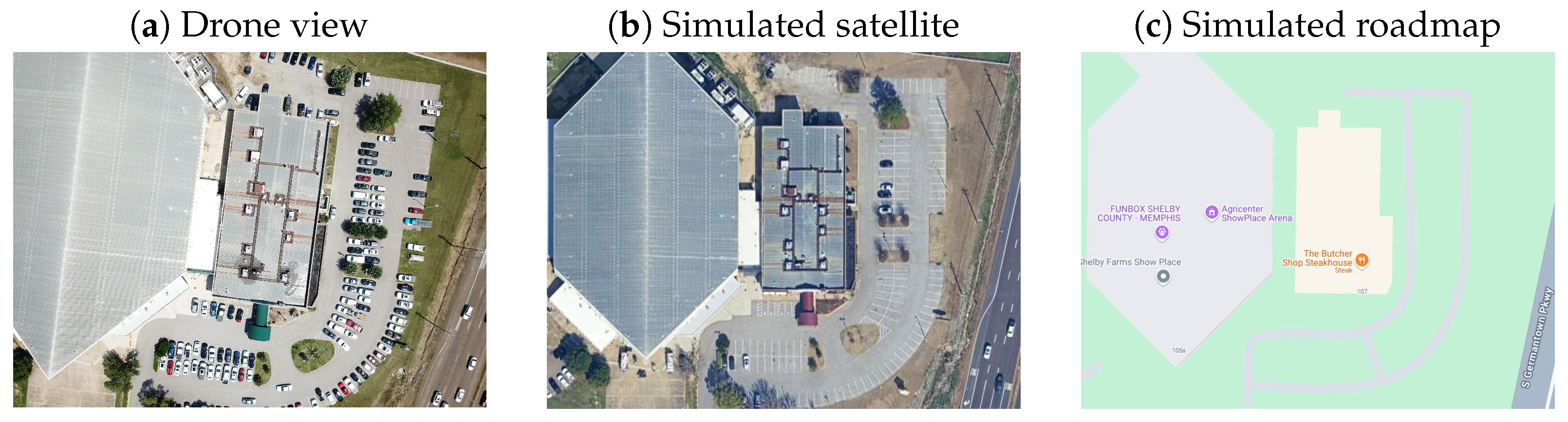
Developing robust machine learning models for aerial imagery applications requires access to large, diverse datasets that ensure both accuracy and generalization [34]. TerrAInav Sim (https://github.com/JacobsSensorLab/TerrAInav-Sim, accessed on 9 April 2025) addresses these needs by providing synthetic aerial datasets that can be used for data augmentation, making it a valuable resource when labeled data are scarce or costly to obtain. This lightweight, versatile tool captures geotagged, simulated aerial images, emulating a UAV capturing bird’s-eye view map-based images with real-world visible-band specifications. By default, the simulated drone is positioned at a zero yaw, facing north, with a 90-degree tilt (looking straight down), as shown in Figure 1. While this orientation is limited to a top-down perspective, it aligns well with many applications that rely on bird’s-eye views for analysis. Through TerrAInav Sim, users can simulate diverse missions by specifying coordinates for any global location using Python 3.10. Additionally, for users with the means to collect their own drone-view images, TerrAInav extends the capabilities of the University1652 dataset to any region, enabling tasks that integrate both drone-view and satellite-view images for enhanced data collection and analysis.
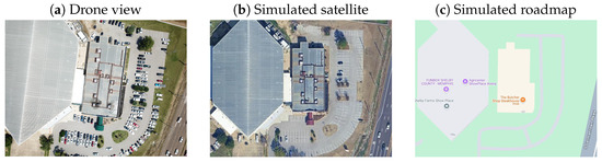
Figure 1.
Image captured at coordinates (35.128039, −89.799163) at above ground level altitude () of 136 m. Image captured (a) by a UAV and simulated (b,c) with a field of view () of 78.8 degrees and aspect ratio () of 4:3. Figures (b,c) represent simulation using different map types.
2. Materials and Methods
In this section, a step-by-step guide will be provided, starting with the theoretical calculations required to define various missions. We will also delve into the architecture of the program, offering an explanation for users to not only utilize but also advance the program to more sophisticated levels.
2.1. Mission Definition
Capturing a single drone image requires collecting all necessary materials and resources similar to a real drone flight, such as altitude and camera settings. Once a single image is captured, we set a solid foundation for more advanced missions. For example, we can program the drone to take multiple images at different locations or complete a raster mission by covering a specified area given the bounding box coordinates.
2.1.1. Single Image Capture
In order to use TerrAInav Sim, some flight and camera parameters have to be known. To capture a single image, these parameters include geodetic latitude and longitude , above ground level altitude in meters (), the diagonal field of view in degrees (), and the imaging aspect ratio of the camera. It is essential to remember that in this version, the camera tilt is 90 degrees, and the drone yaw is 0. In simulations, the digital image pixel size () and zoom level (z) respectfully resemble the and in the real world. Digital dynamic maps load small portions of map data at a time, enabling smooth panning and zooming using the Mercator projection with pixel tiles. Zoom levels range from 0 to 22, organizing tiles in a pyramidal grid where lower zooms show broad geographic features, while higher zooms reveal detailed street and building views. A grid of determines the number of tiles at each zoom level (z). We may use the formula level to find the real size of a single tile on a given zoom level, where is the circumference of the earth (40,075,017 m). Hence, the number of meters per tile side is obtained [35].
The main aspect of this project is to ensure an accurate conversion between the parameters used to specify a flight in the real world versus the ones needed for a virtual image capture. As follows, this section explains how the flight parameters are transformed into the corresponding virtual imaging parameters (z and ). (The functions introduced in the “Single Image Capture” section endnotes are located in the “src/utils” folder within the “geo_helper” package).
To calculate the image diagonal in meters () given and , use the following:
where is a scaler to convert degrees to radians (). Figure 2 illustrates this conversion. Knowing , the width of the map along the x and y axes (, ) in meters can be calculated as follows (the calculations of land size in meters can be performed using the “get_map_dim_m” function):
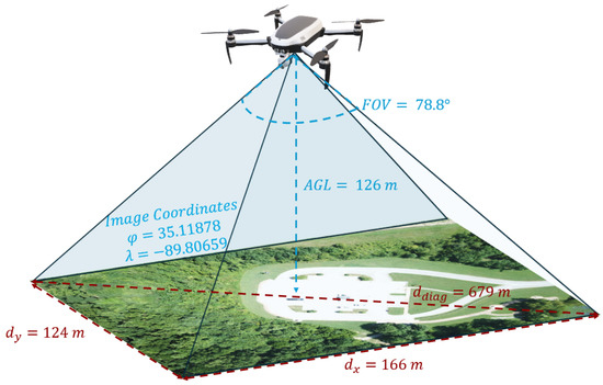
Figure 2.
Image taken by a UAV, with the parameters marked in blue, while the values marked with dark red are calculated. This helps simulate the same experience using satellite data.
Knowing the dimensions in meters, with the benefits of the geopy package [36], the bounding box coordinates will be determined (the process of determining geolocation bounds from metric information is performed by the “calc_bbox_m” function).
If the bounding box is predefined, this step can be bypassed. Then, we have to find the zoom level that maximizes the pixel-wise resolution within a tile. To simulate a geographic area from a central point, zoom level, and map dimensions, we calculate the bounding box coordinates using Mercator projection principles (the “calc_bbox_api” function implements bounding box calculation in Python):
- Center point offset: Offsetting the center point from the center of a web Mercator projection tile according to latitude and longitude ( and ) yields the following [37]:is a constant to scale the longitude from radians to pixels to represent the number of pixels per radian ().
- Bounding Box in Mercator Tile: The map’s resolution in pixels is scaled to the tile in Mercator projection with the help of a scale factor called pixel size. This parameter is calculated from the zoom level (z).Knowing the scaler (), it is also possible to obtain the scaled width and height of the region of interest usingwhere is the resolution in pixels mapped from the real world to the web Mercator projection.
- Convert to coordinates: Convert pixel values to coordinates using the inverse of Equation (3) ( is the top-left () or bottom-right () point.):
Knowing how to calculate the bounding box, it is possible to reverse the process. In the reverse process, the bounding box is known. Hence, the center is known. With the bounds, finding is even easier: . The same applies to the y axis. Reversing Equation (4) give us
Finding the maximum of the resolution’s width and height ensures that the image fits within the selected zoom level in a tile. Using Equations (4) and (5), the resolution of the image within a tile can be measured.
Finally, once the optimal zoom level and the bounding box coordinates are determined, tile coordinates and pixel offsets from the latitude, longitude, and zoom level are calculated, and individual map tiles are retrieved and integrated into a larger stitched image for better pixel resolution. For realistic images, the map type is set to “satellite” by default. However, the program is not limited to capturing realistic images, and different map types can be requested. A flowchart of the process is available in Figure 3. (the “generate_tile_info” takes in the converted information and returns a URL response in the output).
2.1.2. Raster Image Mission
Building on single-image capture, more advanced missions can be defined, such as raster image collection. The main purpose of TerrAInav Sim is to capture raster images of a specified area. In this mission, the objective is to complete a zero-tilt raster image capture, as shown in Figure 4. The capture begins once the bounding box coordinates of the mission’s rectangular region (the map) are set. The coordinates are converted to UTM x and y to facilitate metric calculations and maintain the mission within a rectangular boundary. To ensure the mission remains within one or two UTM zones, it is advisable to restrict its scope to a practical distance. The first image is centered at the top left coordinates of the map. Zoom and image resolution will be calculated from the previous section by inputting the camera , , and the drone’s . By default, images do not overlap, and the distance between consecutive captures equals the image width. Overlap can be introduced by adjusting the spacing using , where is the proportion of shared width/height to the total and has a value between 0 and 1. The mission ends when the bottom right coordinate is captured. The flowchart in Figure 5 represents these steps.
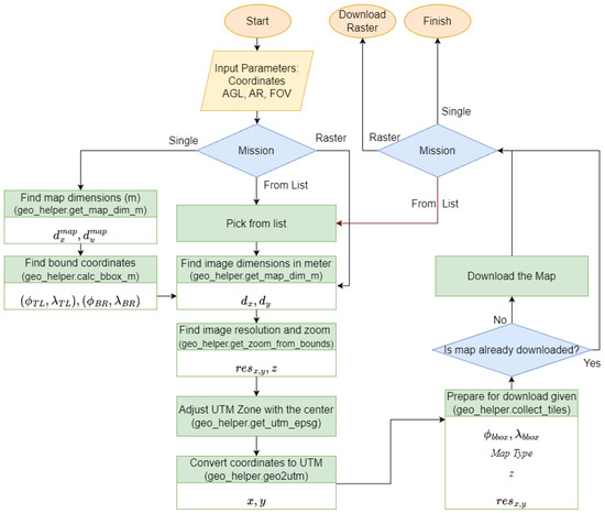
Figure 3.
The flowchart to process the map in downloading picture/s using various missions. Each block includes the name of the function used available in the “src/utils” folder within the “geo_helper” package in parentheses. The “Download Raster” Section refers to the flowchart in Figure 5.
Figure 3.
The flowchart to process the map in downloading picture/s using various missions. Each block includes the name of the function used available in the “src/utils” folder within the “geo_helper” package in parentheses. The “Download Raster” Section refers to the flowchart in Figure 5.

Figure 4.
Raster mission visualization within UTM zone 16 and provided bounding box coordinates.
Figure 4.
Raster mission visualization within UTM zone 16 and provided bounding box coordinates.
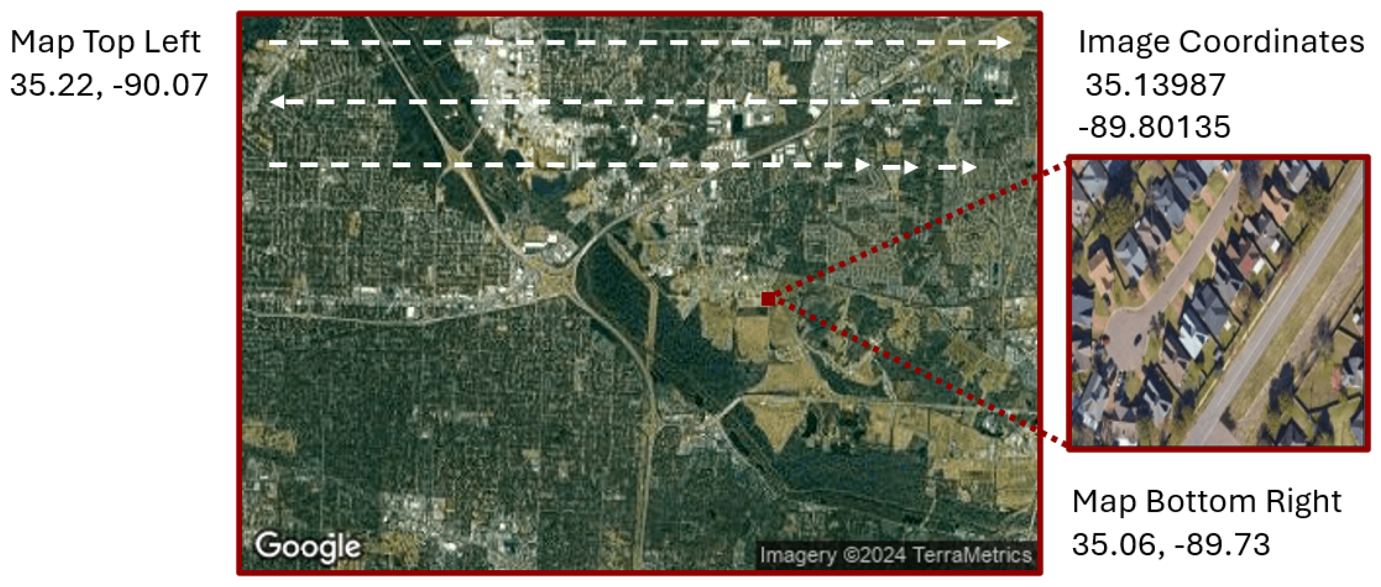
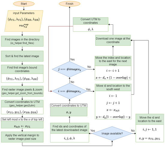
Figure 5.
Raster search image capture flowchart.
Figure 5.
Raster search image capture flowchart.
2.2. Machine Learning PreProcessing
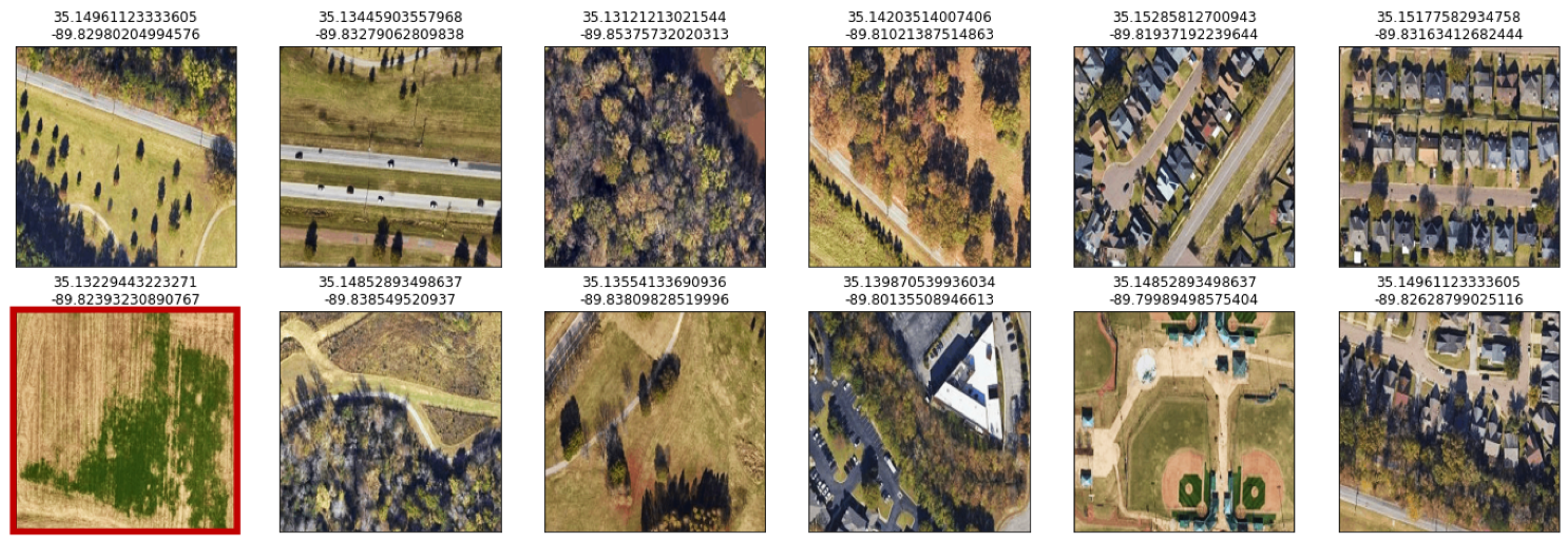
Since machine learning requires a substantial amount of data, raster missions are valuable for providing this dataset. However, not all raster samples may contain useful features for deep learning. Additionally, as the altitude decreases, the likelihood of obtaining featureless images increases. For example, images with dense trees or uniform green areas might not provide sufficient variation or distinct patterns needed for tasks like pattern recognition. In such cases, these images could introduce noise or reduce the effectiveness of the model by not contributing meaningful data. Removing such images ensures that the training dataset contains only relevant and informative samples, leading to better model performance and more accurate results. A few examples in Figure 6 demonstrate this issue.
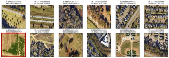
Figure 6.
Satellite mode samples. The image with a red border indicates no significant feature.
Shannon entropy can be used to clean data by identifying and removing samples with insignificant features. It measures the uncertainty or randomness in data, indicating the complexity of an image. High entropy suggests more complexity, while low entropy indicates order [38]. To calculate entropy, conduct the following steps: (1) Convert the image to grayscale; (2) Calculate pixel intensity histogram; (3) Normalize the histogram to get the probability distribution of pixel intensities; (4) Calculate the Shannon entropy using
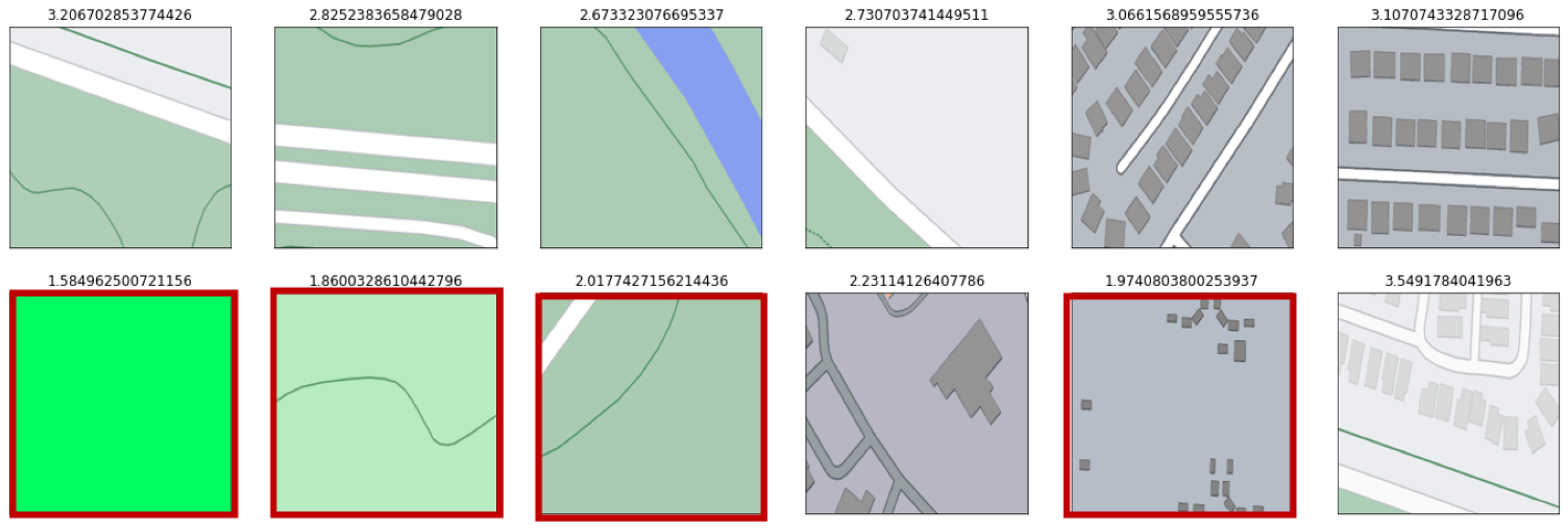
where is the probability of the pixel intensity i. Entropy values help identify samples with fewer significant features. Their values are stored in metadata, and the ones below a certain threshold can be removed later. By looking at the samples in Figure 6 using the roadmap mode (as illustrated in Figure 7), it is easier to detect the ones with fewer significant features.
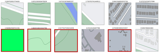
Figure 7.
The same images as in Figure 6 in roadmap mode. In the roadmap, it is easier to detect a lack of significant features, as marked in red. The entropy of each image is marked on top of it.
3. Results
3.1. TerrAInav Dataset
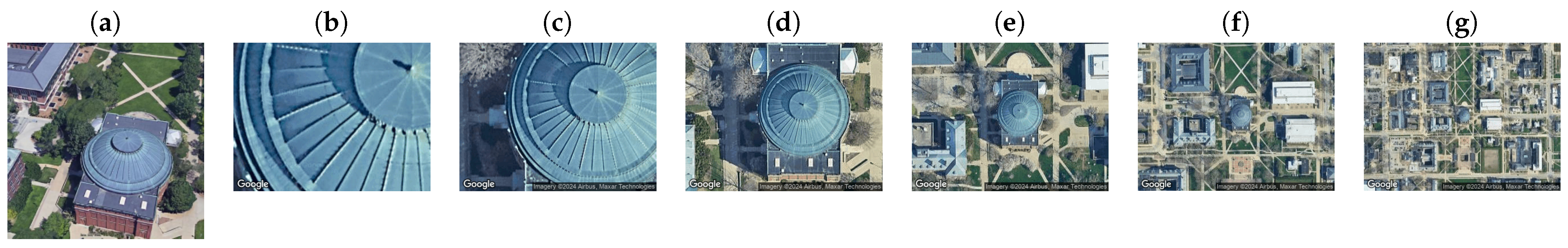
Sample data generated using TerrAInav Sim are available in the ’dataset’ folder. The main dataset, Agricenter dataset, includes raster images of the Memphis Agricenter Area (Figure 8) covering the rectangular bound between the top left coordinates of and the bottom right coordinates of . The simulation uses a UAV-based camera with a of 78.8 degrees, an of 4:3, and a fixed of 120 m. There are two sets of 1806 images each in “satellite” and “roadmap” modes without any overlap. These data are placed in the “Memphis” folder under two subfolders, “satellite” and “roadmap”, specifically designed to be used for machine learning tasks. For ease of access, the images are geotagged; the metadata table contains image names, column and row indices of the raster search, central coordinates of each image, and the zoom level value for each image (“Alt”). A larger dataset generated by TerraAInav Sim from the Memphis area helped with the image feature extraction described in [27]. Some corresponding ML processes will be explained as follows. Figure 9 represents the customizability of the TerrAInav dataset compared to an open-access dataset introduced earlier. In this example, a take-off mission was simulated from the rooftop of the Foellinger Auditorium, University of Illinois Urbana-Champaign, to an altitude of 500 meters.

Figure 8.
Maps representing the area where the raster data have been collected in “satellite” mode on the left and “roadmap” on the right.
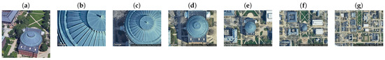
Figure 9.
TerrAInav Sim image capture comparison (b–d) with a sample collected by [13] at 40.10594310015922, −88.22728640012006 (a). The number above each image indicates the captured in meters. All the images were captured with a fov of 78.8 and an aspect ratio of 4:3. (a) 23.8, [13]; (b) 15; (c) 30; (d) 60; (e) 120; (f) 250; (g) 500.
Figure 10 illustrates the capture capabilities at different altitudes and zoom levels, comparing an actual UAV mission to two simulated take-offs from the University of Memphis engineering courtyard to 75 m. The primary differences between the TerrAInav Sim and real-world images include the alignment precision and rotational consistency. The TerrAInav Sim images remain perfectly aligned due to predefined parameters, eliminating errors from sensor inaccuracies, environmental disturbances, and platform instability. In contrast, real-world images show slight misalignment due to GPS drift, IMU noise, wind, and vibrations. This comparison highlights the simulator’s accuracy in replicating aerial imaging while exposing real-world limitations. Figure 1 further demonstrates the simulator’s higher accuracy over actual UAV image capture. Figure 10 also proves that FGFS-generated images fail to accurately represent real-world locations, making them unsuitable for location-specific imaging. Their inferior resolution further limits usability for applications requiring clarity and detail. Moreover, FGFS does not include a built-in automated image capture mechanism, requiring a separate tool. However, given the low image quality—blurriness, low resolution, and absence of geographic and structural details—developing such a tool would be futile. The combination of poor fidelity and missing automation makes FGFS unsuitable for imaging-based applications.
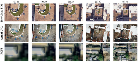
Figure 10.
Image capture comparison using TerrAInav Sim (top row), actual UAV (middle row), and FGFS (bottom row) at 35.12224148, −89.93527809. The captured in meters is indicated above each column. All the images were captured with a fov of 78.8 and an aspect ratio of 4:3. Analysis and quantitative comparison have been provided in Section 3.1.
The courtyard tiles in these images served as a calibration reference for assessing altitude errors at an of 20 m. While both the UAV and the simulator reported an altitude of 20 m, pixel size measurements from the reference images reveal an altitude error of 0.47 m for the UAV image and 0.51 m for the simulated image. Considering the distance between the two error values, the simulator provides a realistic but slightly less precise altitude representation, closely matching real-world UAV measurements.
3.2. Axiliary Dataset
As a source of reference and comparison, a more extensive dataset can be obtained from publicly available road data (https://www.kaggle.com/datasets/parisadkh/terrainav-data, accessed on 9 April 2025). In light of this, we are offering a larger second dataset that covers the city of Memphis. The NVIG, or Night Vision Image Generator, was used to generate terrain for capturing with sensors created in the NVIPM or Night Vision Integrated Performance Model. The OpenStreetMap dataset [39] was used to generate a representation of the Memphis area depicted in Figure 8 for the NVIG. The primary data that OpenStreetMap provides consist of accurate road coordinates. By downloading all the road data within the bounding box coordinates using the QGIS program [40] tools, we obtained shape files which were then parsed to extract the vectors of road coordinates. The most approachable data to extract after the roads are the trees. By creating a threshold function to mask out the regions of map-based imagery of the bounded Memphis area, we can fill the masked regions with random coordinates of varying densities to simulate the presence of trees.
With the road and tree features extracted as series and individual coordinates respectively, the remaining task was generating the appropriate road and tree files for the NVIG to render the features properly. After the tools were developed to automate this, the addition of roads and trees to the NVIG terrain simulation was quick and efficient. However, some caveats that resulted from this technique were artifacts in the road that manifested as sharp and unnatural spikes in the terrain of which the cause has not been discovered. Another problem came from the way roads are generated in the NVIG. The roads are not fitted to the terrain; instead, they are formed by points and try to fit the terrain curvature using a broad slope parameter. A workaround has been to elevate the height of the road so that it is offset some distance above the ground. As most of the imagery is aerial, this does not pose a great issue; however, it would be problematic if imagery were to be collected from ground level. Additionally, the road widths are rarely specified in OpenStreetMap. This forces us to use an arbitrary road width when it is not provided. As a result, the road width is not a reliable metric for feature extraction with the NVIG terrain.
Generating buildings was also a consideration for the NVIG Agricenter terrain dataset; however, the complexity and effort to implement automated building placement in the NVIG deterred us from taking that route. The end result is a medium fidelity 3D representation of the Agricenter terrain over which custom simulated sensors can collect data. Despite the lack of buildings and the occasional road artifacts, the availability of coordinate-accurate roads in a 3D space is powerful in and of itself.
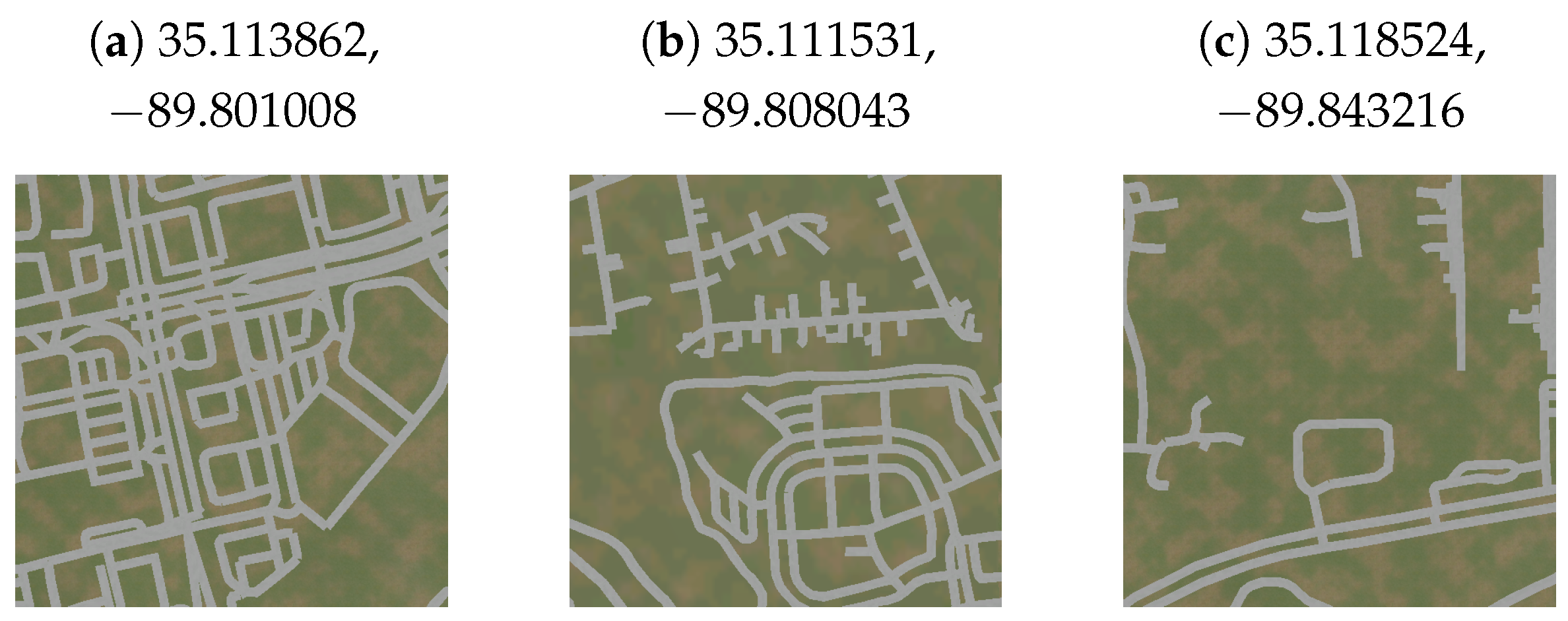
The bounding box for these data has a top-left coordinate of (35.218752, −90.075361) and a bottom-right coordinate of (35.064913, −89.730661). The images are taken in an of 300 m with horizontal and vertical of 75 and make a total of 3350 images. This additional dataset is going to enhance our ability to generate road data and will serve as a key point of comparison with the data from TerrAInav Sim. By comparing the two datasets, we can better assess their strengths and limitations, ultimately improving the accuracy of our machine learning models specifically for road extraction tasks. Figure 11 illustrates one sample of this dataset.
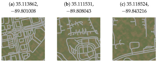
Figure 11.
Sample road data extracted from OpenStreetMap dataset simulated with the NVIPM model. Central coordinates are provided for each sample.
3.3. Postprocessing
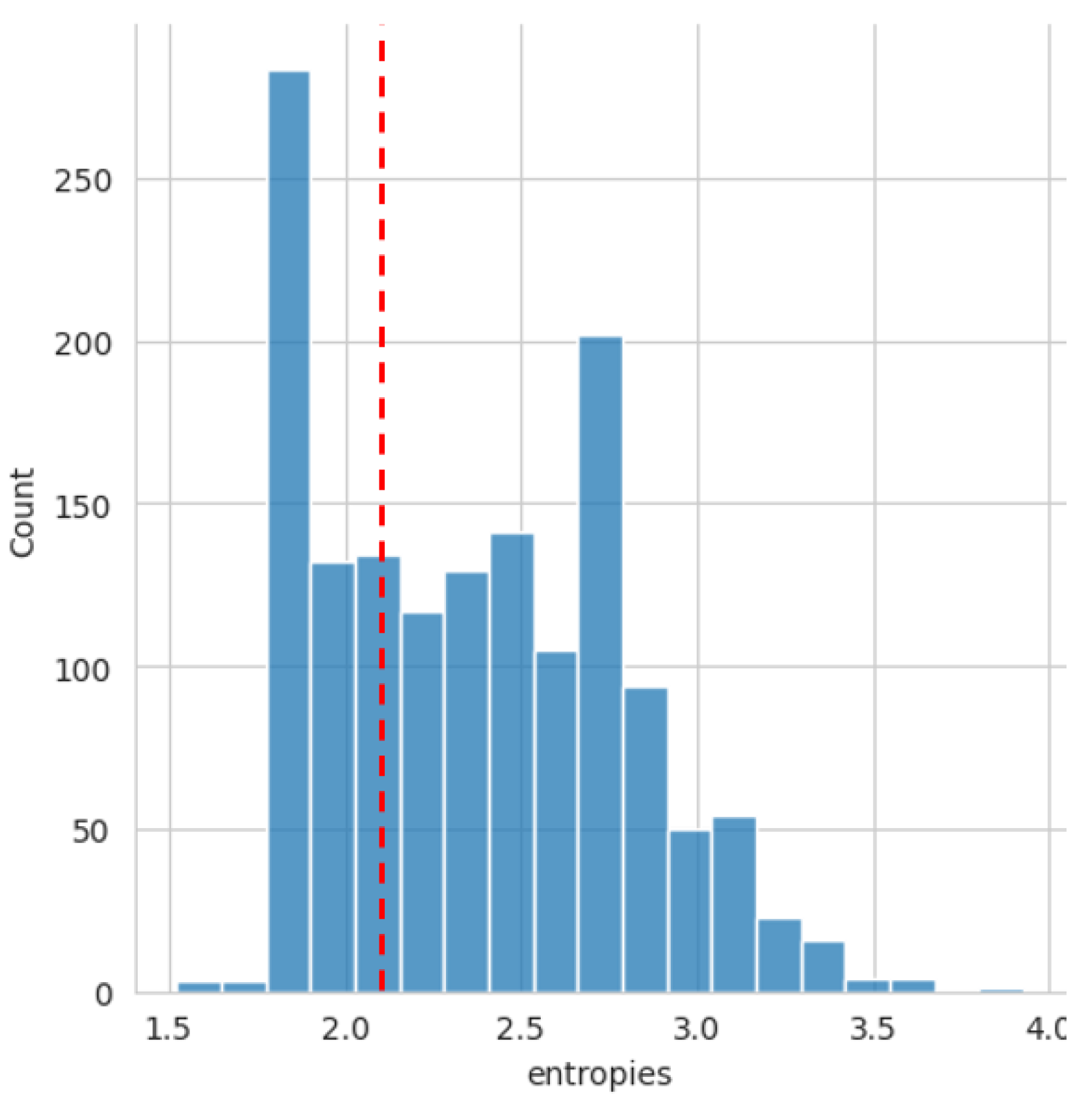
To clean up the data as an optional step, a threshold entropy is defined. The threshold is selected according to the distribution of entropies in all images, along with experimental observations provided in Figure 7. For the Agricenter dataset, images with entropy below 2.1 lack significant details. To validate this threshold and ensure minimal loss of valuable data, Figure 12 presents a histogram of entropies across all roadmap images. This ensures most data are above the threshold, making it safe to discard images below . TerrAInav performs data cleaning based on the selected map type. If the map type is “satellite” or any option other than “roadmap”, the system first checks for the presence of “roadmap” data in the directory. If roadmap images are available, filtering is applied based on their entropy, retaining only those with an entropy above the default threshold (2.1). If no roadmap data exists, filtering is performed directly on the original map type.
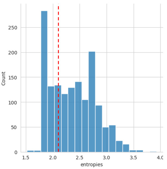
Figure 12.
Histogram of image entropies with the red line marking the 2.1 threshold. As shown, a significant portion of data falls below this threshold, but these samples mostly consist of unremarkable features, like green areas with trees and farms. Discarding them is ideal, as the majority of valuable data remains safely above the threshold.
Roadmaps inherently contain less texture and color variation compared to satellite images, making key features such as roads, buildings, and intersections stand out more clearly. Entropy, as a measure of information content, assigns higher values to images with a diverse range of distinct features, such as dense urban areas or complex street networks. Since roadmaps lack environmental noise commonly found in satellite imagery—such as shadows, vegetation, and natural terrain—entropy provides a more direct indication of structured, meaningful information. High entropy in a roadmap image suggests a rich presence of human-made elements rather than uninformative background textures, which are more prevalent in satellite images. Consequently, TerrAInav minimizes the risk of overfitting to redundant or uninformative patterns, ensuring that the model focuses on more complex and distinctive elements.
After the data are cleaned using the “cleanup_data” method, the “config_dnn” method can be called to prepare the dataset for a machine learning task. In this process, the labels are the central latitude and longitude of each image, which are then converted to UTM and normalized using a standard scaler. These data are then split into three sets: train, validation, and test. At this stage, the cleaned data are transferred to a Keras dataset [41], where they are preprocessed and divided into batches. Data augmentation is then applied, including random rotation, flip, and zoom by default. Additional options like random contrast and brightness adjustments are also available if needed.
3.4. Performance
The tool’s performance has been evaluated across a diverse range of environments, including low-end laptops and high-performance GPU servers running on Linux and Windows operating systems. The reported results reflect an averaged performance across these varied settings to demonstrate its versatility. TerrAInav Sim demonstrates robust computational efficiency, with an average preparation time of 0.19 s and a maximum memory usage of 250 MBs that showcases comparably faster and more efficient performance than other simulation tools, as referenced in Table 2.
Table 2.
Performance comparison in case of runtime, memory, and functionality between TerrAInav Sim and other simulators. Preparation time is the time needed to initialize the program, load dependencies, set parameters, and ensure readiness for image capture.
The performance analysis highlights the simulator’s capability to capture images across a wide range of ground sampling distances (GSDs), from large-scale city-wide retrievals to high-resolution, low-altitude captures. In city-wide imaging, where the altitude is significantly higher, the GSD values ranged from approximately 125 m/pixel to 0.98 m/pixel, with larger images taking longer to retrieve—up to 27.59 ms for the highest resolution, as illustrated in Table 3.
Table 3.
Performance analysis of city-wide image retrieval using TerrAInva Sim located within the bounds of (35.19, −89.94) and (35.11, −89.8).
On the other hand, at the lowest achievable altitude (7 m ), the GSD reached as fine as 0.03 m/pixel (Table 4), demonstrating the simulator’s ability to capture highly detailed imagery. The retrieval times in this low-altitude scenario remained relatively stable, ranging from 0.19 ms to 0.30 ms, indicating that image size plays a more significant role in retrieval time than altitude alone. This flexibility in image acquisition allows the simulator to balance resolution needs with processing efficiency, making it suitable for applications requiring both broad spatial coverage and detailed close-range observations. For typical raster missions at 120 m altitude and an average resolution of 640 × 480, the retrieval time averaged 0.15 s per image, demonstrating practical performance for large-scale aerial surveying tasks.
Table 4.
Performance analysis of an image retrieved at an of 7 m located within the bounds of (35.12188469, −89.93491779) and (35.12181490, −89.93481732). This is an example of the lowest achievable by TerrAInva Sim.
The storage requirements per image were minimal: large roadmap images (9120 × 13,049 resolution) required up to 272 KB, while satellite images remained under 462 KB. The storage requirement for a typical 640 × 480 image was, however, no more than 110 KBs for satellite and 16 KBs for roadmap images, allowing for efficient storage even in large-scale applications. Notably, this is significantly more efficient than images acquired by a Mavic drone, which has a maximum resolution of 4000 × 3000, yet each image requires more than 4 MB of storage. This demonstrates the advantages of our approach in terms of storage efficiency, particularly for large-scale and resource-constrained applications. This flexibility also allows TerrAInav Sim to scale effectively across different network environments while maintaining efficient use of system resources.
4. Discussion
TerrAInav Sim opens the door to numerous applications, but it does have limitations that could affect its utility in certain scenarios. One notable limitation arises from the reliance on the Google Maps Static API, which prevents the determination of the exact date of the imagery. This can lead to discrepancies in temporal accuracy, especially in applications where precise timestamping is crucial, such as change detection in environmental monitoring or tracking land use over time in agricultural applications. This limitation, while not critical for most of TerrAInav Sim’s potential applications, is still an important area for future improvement. To address this limitation, a potential solution is to integrate additional data sources that provide timestamped satellite imagery. For instance, services like Google Earth Engine [42] offer access to historical satellite imagery with precise timestamps, which could be leveraged through their APIs. However, their archive still has its own limitations. Integrating these services into TerrAInav Sim would significantly improve the temporal accuracy of the imagery, making the tool more suitable for applications that require historical comparisons, event tracking, or temporal analysis.
Another limitation lies in the idealized nature of the simulation, which does not account for the complexities and inaccuracies typical of real-world drone missions. Factors such as sensor faults, varying environmental conditions, and obstacles like buildings or trees can significantly impact the quality of images captured during actual operations. For example, in tasks like urban mapping or vegetation analysis, these inaccuracies could introduce errors in feature extraction or object recognition. Currently, TerrAInav Sim provides a controlled, distortion-free environment, but this does not reflect the unpredictability of real-world operations. To mitigate this, incorporating error models simulating sensor noise, dynamic obstacles, and environmental factors (e.g., wind or lighting changes) could better represent real-world conditions. This would allow users to assess how their systems would perform in diverse, unpredictable scenarios, which is particularly important for applications like environmental monitoring or disaster response.
The current simulator also uses a high-altitude image capture and cropping method to simulate low-altitude drone behavior. While the proposed approach provides a reasonable approximation, it does not replicate the distortions and misalignments experienced during actual low-altitude flights. This discrepancy can be particularly problematic in applications requiring precise 3D modeling or when operating in densely built-up areas where buildings can create severe perspective distortions. To address this, future versions of the simulator could implement custom distortion models that account for terrain elevation, building height, and the specific angle of capture. This would allow for more realistic simulations of low-altitude operations, improving the accuracy of applications like urban modeling or emergency response planning.
Furthermore, there is a trade-off between image quality and processing speed. High-quality images require more computational resources, which can increase processing time, potentially limiting the simulator’s utility in real-time applications, such as autonomous navigation or obstacle avoidance in dynamic environments. On the other hand, faster image acquisition and processing can lead to a reduction in image fidelity, which may compromise the accuracy of object detection and map generation. In future versions, a dynamic adjustment system that optimizes the balance between image quality and processing speed, perhaps based on the specific needs of the task at hand (e.g., prioritizing speed for real-time navigation vs. quality for detailed mapping), could provide a more flexible and practical solution for users.
Lastly, the current image capture setup, which limits yaw to zero and tilt to 90 degrees, restricts the available angles for data capture. This limitation is particularly restrictive in applications that require a full 360-degree view for accurate environmental modeling or surveillance. Expanding the simulator to include dynamic adjustments for both yaw and tilt would allow for a broader range of angles, enabling more comprehensive data capture for tasks like infrastructure inspection, where capturing multiple angles of a structure is essential for thorough analysis.
5. Conclusions
TerrAInav Sim’s functionality allows users to customize various parameters, including flight altitude, camera aspect ratio, diagonal field of view, and image overlap. This flexibility supports a wide range of applications, from capturing low-altitude images for simple tasks to generating comprehensive datasets for complex projects. The ability to quickly and efficiently capture large volumes of images while utilizing minimal memory makes it an ideal candidate for deep learning. Its potential applications span various fields, including classification, pattern recognition, localization, and image-to-image translation, showcasing just a few of its capabilities in deep learning. By offering a faster and simpler alternative to commercial flight simulators, TerrAInav Sim accelerates experimentation and validation processes, making it an invaluable resource for future advancements in UAV-based geospatial analysis, environmental monitoring, and autonomous navigation research.
In addition to its versatility, TerrAInav Sim’s open-source nature encourages further development and adaptation to other missions beyond its initial design. The tool’s ability to produce extensive datasets without the need for physical UAV deployment represents a significant advancement in dataset generation for VBN algorithm developments. TerrAInav Sim presents a compelling solution to the challenges of aerial image capture, offering a powerful and flexible tool for a variety of applications and opening new avenues for research and development in VBN and beyond.
By providing a customizable, cost-effective tool for generating diverse image datasets, TerrAInav Sim lowers barriers to entry for research in autonomous navigation, environmental monitoring, and urban planning. Its open-source nature encourages continued development, making it a valuable asset for advancing machine learning and remote sensing applications.
Author Contributions
Conceptualization, S.P.D.; Data curation, S.P.D., P.M.L. and O.F.; Formal analysis, S.P.D., P.M.L. and O.F.; Funding acquisition, E.L.J.; Investigation, S.P.D., P.M.L. and O.F.; Methodology, S.P.D.; Project administration, E.L.J.; Resources, S.P.D., P.M.L. and O.F.; Software, S.P.D., P.M.L. and O.F.; Supervision, E.L.J. and O.F.; Validation, S.P.D., E.L.J., P.M.L. and O.F.; Visualization, S.P.D.; Writing—original draft, S.P.D.; Writing—review and editing, S.P.D., E.L.J. and P.M.L. All authors have read and agreed to the published version of the manuscript.
Funding
Research was sponsored by the Army Research Laboratory and was accomplished under Cooperative Agreement Number W911NF-21-2-0192. The views and conclusions contained in this document are those of the authors and should not be interpreted as representing the official policies, either expressed or implied, of the Army Research Office or the U.S. Government. The U.S. Government is authorized to reproduce and distribute reprints for Government purposes, notwithstanding any copyright notation herein.
Data Availability Statement
TerrAInav Sim Python program will be available at https://github.com/JacobsSensorLab/TerrAInav-Sim, accessed on 9 April 2025. The data are also separately available at https://www.kaggle.com/datasets/parisadkh/terrainav-data/data, accessed on 9 April 2025.
Acknowledgments
We would like to extend my sincere thanks to our colleagues at the Jacobs Sensor Lab and the Center for Applied Earth Science and Engineering Research (CAESER) for their invaluable support and collaboration throughout this work. Their insights and contributions have greatly enhanced this research.
Conflicts of Interest
There is no conflict of interest.
References
- Zhang, X.; He, Z.; Ma, Z.; Wang, Z.; Wang, L. LLFE: A novel learning local features extraction for UAV navigation based on infrared aerial image and satellite reference image matching. Remote Sens. 2021, 13, 4618. [Google Scholar] [CrossRef]
- Liang, C.W.; Zheng, Z.C.; Chen, T.N. Monitoring landfill volatile organic compounds emissions by an uncrewed aerial vehicle platform with infrared and visible-light cameras, remote monitoring, and sampling systems. J. Environ. Manag. 2024, 365, 121575. [Google Scholar] [CrossRef] [PubMed]
- Liu, W.; Zhou, L.; Zhang, S.; Luo, N.; Xu, M. A new High-Precision and Lightweight Detection Model for illegal construction objects based on deep learning. Tsinghua Sci. Technol. 2024, 29, 1002–1022. [Google Scholar] [CrossRef]
- Cao, Y.; Yu, X.; Jiang, F. Application of 3D image technology in rural planning. ACM Trans. Asian Low-Resour. Lang. Inf. Process. 2024, 23, 1–13. [Google Scholar] [CrossRef]
- Gąsienica-Józkowy, J.; Knapik, M.; Cyganek, B. An ensemble deep learning method with optimized weights for drone-based water rescue and surveillance. Integr. Comput. Aided Eng. 2021, 28, 221–235. [Google Scholar] [CrossRef]
- Long, J.; Shelhamer, E.; Darrell, T. Fully Convolutional Networks for Semantic Segmentation. arXiv 2015, arXiv:1411.4038. [Google Scholar]
- Guo, Y.; Xiao, Y.; Hao, F.; Zhang, X.; Chen, J.; de Beurs, K.; He, Y.; Fu, Y.H. Comparison of different machine learning algorithms for predicting maize grain yield using UAV-based hyperspectral images. Int. J. Appl. Earth Obs. Geoinf. 2023, 124, 103528. [Google Scholar] [CrossRef]
- Sainte Fare Garnot, V.; Landrieu, L. Panoptic Segmentation of Satellite Image Time Series with Convolutional Temporal Attention Networks. In Proceedings of the 2021 IEEE/CVF International Conference on Computer Vision (ICCV), Montreal, QC, Canada, 10–17 October 2021. [Google Scholar]
- Ban, Y.; Yousif, O. Change Detection Techniques: A Review. In Multitemporal Remote Sensing; Springer: Berlin/Heidelberg, Germany, 2016; pp. 19–43. [Google Scholar] [CrossRef]
- Yang, S.Y.; Cheng, H.Y.; Yu, C.C. Real-Time Object Detection and Tracking for Unmanned Aerial Vehicles Based on Convolutional Neural Networks. Electronics 2023, 12, 4928. [Google Scholar] [CrossRef]
- Christoph, R. GitHub—Chrieke/Awesome-Satellite-Imagery-Datasets: List of Satellite Image Training Datasets with Annotations for Computer Vision and Deep Learning—github.com. 2022. Available online: https://github.com/chrieke/awesome-satellite-imagery-datasets (accessed on 13 August 2024).
- Rahnemoonfar, M.; Chowdhury, T.; Sarkar, A.; Varshney, D.; Yari, M.; Murphy, R.R. FloodNet: A High Resolution Aerial Imagery Dataset for Post Flood Scene Understanding. IEEE Access 2021, 9, 89644–89654. [Google Scholar] [CrossRef]
- Zheng, Z.; Wei, Y.; Yang, Y. University-1652: A Multi-view Multi-source Benchmark for Drone-based Geo-localization. ACM Multimed. 2020, arXiv:2002.12186. [Google Scholar]
- Zheng, Z.; Shi, Y.; Wang, T.; Liu, J.; Fang, J.; Wei, Y.; Chua, T.S. UAVM’23: 2023 Workshop on UAVs in Multimedia: Capturing the World from a New Perspective. In Proceedings of the 31st ACM International Conference on Multimedia, Ottawa, ON, Canada, 29 October 2023–3 November 2023; pp. 9715–9717. [Google Scholar]
- Xia, G.S.; Hu, J.; Hu, F.; Shi, B.; Bai, X.; Zhong, Y.; Zhang, L.; Lu, X. AID: A Benchmark Data Set for Performance Evaluation of Aerial Scene cls. IEEE Trans. Geosci. Remote Sens. 2017, 55, 3965–3981. [Google Scholar] [CrossRef]
- Demir, I.; Koperski, K.; Lindenbaum, D.; Pang, G.; Huang, J.; Basu, S.; Hughes, F.; Tuia, D.; Raskar, R. DeepGlobe 2018: A Challenge to Parse the Earth through sat. Images. In Proceedings of the 2018 IEEE/CVF Conference on Computer Vision and Pattern rec. Workshops (CVPRW), Salt Lake City, UT, USA, 18–22 June 2018. [Google Scholar] [CrossRef]
- Waqas Zamir, S.; Arora, A.; Gupta, A.; Khan, S.; Sun, G.; Shahbaz Khan, F.; Zhu, F.; Shao, L.; Xia, G.S.; Bai, X. iSAID: A Large-scale Dataset for Instance seg. in Aerial Images. In Proceedings of the IEEE Conference on Computer Vision and Pattern rec. Workshops, Long Beach, CA, USA, 16–17 June 2019; pp. 28–37. [Google Scholar]
- Xia, G.S.; Bai, X.; Ding, J.; Zhu, Z.; Belongie, S.; Luo, J.; Datcu, M.; Pelillo, M.; Zhang, L. DOTA: A Large-Scale Dataset for Object Detection in Aerial Images. In Proceedings of the IEEE Conference on Computer Vision and Pattern rec. (CVPR), Salt Lake City, UT, USA, 18–22 June 2018. [Google Scholar]
- Maryam, R.; Tashnim, C.; Robin, M. RescueNet: A High Resolution UAV Semantic Segmentation Dataset for Natural Disaster Damage Assessment. Sci. Data 2023, 10, 913. [Google Scholar] [CrossRef]
- Ding, J.; Xue, N.; Xia, G.S.; Bai, X.; Yang, W.; Yang, M.; Belongie, S.; Luo, J.; Datcu, M.; Pelillo, M.; et al. Object Detection in Aerial Images: A Large-Scale Benchmark and Challenges. IEEE Trans. Pattern Anal. Mach. Intell. 2021, 44, 7778–7796. [Google Scholar] [CrossRef] [PubMed]
- Ding, J.; Xue, N.; Long, Y.; Xia, G.-S.; Liu, Q. Learning RoI Transformer for Detecting Oriented objects in Aerial Images. In Proceedings of the IEEE Conference on Computer Vision and Pattern rec. (CVPR), Long Beach, CA, USA, 15–20 June 2019. [Google Scholar]
- Workman, S.; Souvenir, R.; Jacobs, N. Wide-Area Image Geolocation with Aerial Reference Imagery. In Proceedings of the IEEE International Conference on Computer Vision (ICCV), Santiago, Chile, 7–13 December 2015; pp. 1–9. [Google Scholar] [CrossRef]
- Christie, G.; Fendley, N.; Wilson, J.; Mukherjee, R. Functional Map of the World. In Proceedings of the CVPR, Salt Lake City, UT, USA, 18–23 June 2018. [Google Scholar]
- Liu, L.; Li, H. Lending Orientation to Neural Networks for Cross-view Geo-loc. arXiv 2019, arXiv:1903.12351. [Google Scholar]
- Helber, P.; Bischke, B.; Dengel, A.; Borth, D. Introducing EuroSAT: A Novel Dataset and Deep Learning Benchmark for Land Use and Land Cover cls. In Proceedings of the IGARSS 2018—2018 IEEE International Geoscience and Remote Sensing Symposium, Valencia, Spain, 22–27 July 2018; pp. 204–207. [Google Scholar]
- Requena-Mesa, C.; Benson, V.; Reichstein, M.; Runge, J.; Denzler, J. EarthNet2021: A large-scale dataset and challenge for Earth surface forecasting as a guided video prediction task. arXiv 2021, arXiv:2104.10066. [Google Scholar]
- Dajkhosh, S.P.; Furxhi, O.; Renshaw, C.K.; Jacobs, E.L. Aerial image feature mapping using deep neural networks. In Proceedings of the Geospatial Informatics XIV; Palaniappan, K., Seetharaman, G., Eds.; International Society for Optics and Photonics, SPIE: National Harbor, MD, USA, 2024; Volume PC13037, p. PC1303701. [Google Scholar] [CrossRef]
- Liu, R.; Wu, J.; Lu, W.; Miao, Q.; Zhang, H.; Liu, X.; Lu, Z.; Li, L. A Review of Deep Learning-Based Methods for Road Extraction from High-Resolution Remote Sensing Images. Remote Sens. 2024, 16, 2056. [Google Scholar] [CrossRef]
- Si, J.; Kim, S. GAN-Based Map Generation Technique of Aerial Image Using Residual Blocks and Canny Edge Detector. Appl. Sci. 2024, 14, 10963. [Google Scholar] [CrossRef]
- Microsoft Corporation. Microsoft Flight Simulator. Available online: https://www.flightsimulator.com/ (accessed on 4 November 2024).
- Flight Gear. FlightGear Flight Simulator. Available online: https://www.flightgear.org/ (accessed on 4 November 2024).
- Tassin, X. GeoFS—Free Online Flight Simulator—geo-fs.com. Available online: https://www.geo-fs.com/ (accessed on 4 November 2024).
- Derekhe. GitHub—Derekhe/msfs2020-map-enhancement—github.com. 2024. Available online: https://github.com/derekhe/msfs2020-map-enhancement (accessed on 16 January 2025).
- Sun, C.; Shrivastava, A.; Singh, S.; Gupta, R. Revisiting unreasonable effectiveness of data in deep learning era. In Proceedings of the IEEE International Conference on Computer Vision, Venice, Italy, 22–29 October 2017; pp. 843–852. [Google Scholar]
- Understanding Zoom Level in Maps and Imagery— support.plexearth.com. Available online: https://support.plexearth.com/hc/en-us/articles/6325794324497-Understanding-Zoom-Level-in-Maps-and-Imagery (accessed on 26 August 2024).
- GeoPy. Geopy: Geocoding Library for Python; GitHub: San Francisco, CA, USA, 2024; Version 2.3.0. [Google Scholar]
- Osborne, P. The Mercator Projections; Normal Mercator on the Sphere: NMS; Zenodo: Geneva, Switzerland, 2013. [Google Scholar] [CrossRef]
- Shannon, C.E. A Mathematical Theory of Communication. Bell Syst. Tech. J. 1948, 27, 379–423. [Google Scholar] [CrossRef]
- OpenStreetMap—openstreetmap.org. Available online: https://www.openstreetmap.org/#map=5/38.01/-95.84 (accessed on 26 August 2024).
- QGIS.org. QGIS Geographic Information System. Open Source Geospatial Foundation Project. Available online: http://qgis.org (accessed on 9 April 2025).
- Chollet, François and Others Keras Documentation: Datasets—keras.io. Available online: https://keras.io/api/datasets/ (accessed on 3 September 2024).
- Python Installation |Google Earth Engine |Google for Developers—developers.google.com. Available online: https://developers.google.com/earth-engine/guides/python_install (accessed on 26 August 2024).


Disclaimer/Publisher’s Note: The statements, opinions and data contained in all publications are solely those of the individual author(s) and contributor(s) and not of MDPI and/or the editor(s). MDPI and/or the editor(s) disclaim responsibility for any injury to people or property resulting from any ideas, methods, instructions or products referred to in the content. |
© 2025 by the authors. Licensee MDPI, Basel, Switzerland. This article is an open access article distributed under the terms and conditions of the Creative Commons Attribution (CC BY) license (https://creativecommons.org/licenses/by/4.0/).