Spatial and Temporal Characteristics of Mesoscale Eddies in the North Atlantic Ocean Based on SWOT Mission

Abstract

Mesoscale eddies play a crucial role as primary transporters of heat, salinity, and freshwater in oceanic systems. Utilizing the latest Surface Water and Ocean Topography (SWOT) dataset, this study employed the py-eddy-tracker (PET) algorithm to identify and track mesoscale eddies in the North Atlantic (NA). Our investigation focused on evaluating the influence of applying varying filter wavelengths (800, 600, 400, and 200 km) for absolute dynamic topography (ADT) on the detection of spatiotemporal patterns and dynamic properties of mesoscale eddies, encompassing eddy kinetic energy (EKE), effective radius, rotational velocity, amplitude, lifespan, and propagation distance. The analysis reveals a cyclonic to anticyclonic eddy ratio of approximately 1.1:1 in the study region. The dynamic parameters of mesoscale eddies identified at filter wavelengths of 800 km and 600 km are similar, while a marked reduction in these parameters becomes evident at the 200 km wavelength. Parameter comparative analysis indicates that effective radius exhibits the highest sensitivity to wavelength reduction, followed by amplitude, whereas rotational velocity remains relatively unaffected by filtering variations. The lifespan distribution analysis shows that the majority of eddies persist for 7–21 days, with only a small number of robust mesoscale eddies maintaining activity beyond 45 days. These long-lived, strong mesoscale eddies are primarily generated in the high-energy current zones associated with the Gulf Stream (GS).

1. Introduction

The ocean circulation system integrates the ocean, which covers 70 percent of the Earth’s surface, and regions of strong currents often exhibit high instability, providing the fundamental conditions for the formation of mesoscale eddies [1]. Major oceanic dynamic processes include large-scale (>500 km), mesoscale (50–500 km), and submesoscale (1–50 km) structures, with most energy concentrated in the geostrophic eddy field [2]. Studies based on satellite observations have shown that mesoscale eddies contribute to 80 percent of the ocean’s total kinetic energy [3,4]. Mesoscale eddies typically extend over tens to hundreds of kilometers and have lifetimes ranging from several tens to several hundred days. These eddies play a crucial role in ocean dynamics by transporting heat, salinity, freshwater, plankton, and other materials, thereby influencing the exchange of gases and nutrients between the surface and deep ocean. This makes them essential for understanding the ocean’s role in regulating climate change [5,6,7,8,9,10]. The dynamic parameters of eddies, such as amplitude, effective radius, and rotational velocity, provide valuable insights into atmospheric and oceanic dynamics, as well as related climate and weather phenomena. The amplitude generally reflects the eddy’s intensity, with larger amplitudes indicating stronger destructive potential. The effective radius describes the eddy’s area of influence, aiding in the evaluation of its potential impacts on the atmosphere–ocean system. Rotational velocity, on the other hand, indicates the energy distribution and developmental trends of the eddy.

The generation of eddies is influenced by various factors, including wind stress, topographic effects (such as submarine mountains and trenches), and tidal effects. Among these, baroclinic instability is recognized as the primary mechanism driving the formation of mesoscale eddies [11]. Mesoscale eddies are generally categorized into two types: cyclonic eddy (CE) and anticyclonic eddy (AE). CE systems are low-pressure systems that typically rotate counterclockwise in the northern hemisphere. They are often referred to as “cold eddies” due to the upwelling of deep water, which results in cooling of the sea surface temperature in their central regions. In contrast, AE systems are high-pressure systems that rotate clockwise in the northern hemisphere. The downwelling currents in their central regions cause the surface water to sink, leading to an increase in sea surface temperature (SST), hence the name “warm eddy”. While an eddy represents a localized rotational phenomenon, circulation describes the overall rotational effect along the closed path, with the two closely related through the flow properties of the fluid. Areas with notable sea surface fluctuations are generally associated with strong circulation activity and high eddy kinetic energy (EKE), meaning that regions of intense circulation often feature robust eddy activity. In such regions, the continuous formation and dissipation of eddies play a critical role in global climate change by affecting the ocean’s temperature and salinity distribution.The CE and AE in the North Atlantic(NA) exhibit distinct temporal and spatial characteristics and collectively shape the ocean dynamics of the region.

The Gulf Stream (GS) originates in the Gulf of Mexico and flows northward, significantly influencing the temperature and salinity distribution of the ocean. This warm current not only regulates the physical environment but is also closely related to eddy activity. As a result, previous studies on eddies in the Gulf of Mexico [12,13,14], particularly focusing on the surface and three-dimensional characteristics of these eddies, have received considerable attention. However, due to the insufficient spatial coverage and resolution of satellite data, the analysis of the temporal and spatial characteristics of eddies across the NA remains inadequate, with research primarily focused on specific regions. Aguedjou et al. [15] analyzed the characteristics of eddies in the tropical Atlantic Ocean (TAO) by using the sea surface height (SSH) data measured by multi-source satellite altimeters over the past 20 years (1993–2012). A large number of eddies were observed in the eastern TAO, and up to 120 eddies could be identified per square degree per year, with amplitudes ranging from 1–6 cm. The radius of the eddy is generally 60–90 km, and the EKE of the eddy is weak, less than 150 cm. With a lifetime of over 16 weeks, the percentage of CE and AE with a radius greater than or equal to 18 km were nearly equal [16]. Kang et al. [17] used high-resolution regional ocean models to study eddies in the GS and found that the CE in this area are smaller in scale than the AE, yet they possess stronger energy and longer durations. Early research on eddies mainly relied on traditional oceanographic methods, which were constrained by the spatial and temporal resolution of the observational data.

The earliest detailed observations of mesoscale eddies date back to the pioneering exploration programs POLYGON-70 and MODE-1 in the early 1970s [18]. The advent of satellite altimetry technology has revolutionized the study of the global ocean. The current altimetry systems have exceeded expectations in monitoring and understanding ocean dynamic processes at the mesoscale and larger scales, substantially advancing the understanding of global ocean circulation and sea level changes [19,20,21]. Using altimetric data from the Topex/Poseidon (T/P) satellite, Stammer et al. [22,23] identified a distinct geographical heterogeneity in the EKE distribution of the NA. The highest EKE was observed in boundary current regions, with high-energy bands extending inward along frontal structures and the ocean circulation system, while the lowest EKE occurred in the mid-latitude range of 37°N to 47°N. Brachet et al. [24] calculated that the spatial scale of eddies in the NA (280°E–360°E, 25°N–50°N) ranged from approximately 100 to 200 km using T/P and ERS-1/2 satellite altimetry data and the Parallel Ocean Program (POP) model. The spatial scale variation was found to correlate with the deformation radius of Rossby waves, which decrease with increasing latitude. Recent studies have revealed that smaller-scale ocean eddies (1–50 km) are more energetic than previously thought, playing a critical role in ocean energy cascades and vertical mass transport [3,25,26,27]. However, the spatial resolution of SSH data from traditional altimeters is limited by coarse satellite orbit sampling and instrument errors, making it challenging to observe high-resolution small-scale ocean dynamics [28]. The Surface Water and Ocean Topography (SWOT) mission, launched in December 2022, offers high-resolution observations of SSH, presenting new opportunities for studying small- and medium-scale eddies.

The SWOT satellite is a groundbreaking mission utilizing radar interferometry [28], enabling high-resolution, wide-swath sea surface observations. The core instrument of the SWOT satellite is the Ka-band Radar Interferometer (KaRIn), which extends traditional one-dimensional profile observations to two-dimensional mapping, achieving a spatial resolution of 2 km with a 21-day revisit period [29]. The satellite’s 120-km-wide swath (with a 20-km-wide nadir gap sampled by the subsatellite point altimeter) will provide coverage for more than 90 percent of the global ocean surface [30]. The primary oceanographic objective of the SWOT mission is to characterize mesoscale and submesoscale phenomena in the ocean at spatial resolutions of 15 km or higher, facilitating the observation of smaller-scale oceanic dynamic processes. This advancement holds the potential to improve climate prediction models and uncover new insights into material transport within the ocean.

In this study, mesoscale eddies in the NA (280°E–350°E, 25°N–50°N) are identified and tracked using AVISO datasets integrated with the latest observations from the SWOT satellite. A Bessel filter was applied to identify mesoscale eddies through high-pass filtering of datasets processed with 800 km, 600 km, 400 km, and 200 km filter wavelengths. Variations in mesoscale eddies identified at different filter wavelengths were examined, and the similarities and differences in various eddy parameters across these scales were analyzed. Parameters such as EKE, amplitude, radius, rotation speed, and propagation distance were selected to reveal the spatiotemporal distribution characteristics of mesoscale eddies.

2. Study Area

The NA (280°E–350°E, 25°N–50°N) was selected as the research area in this study. As shown in Figure 1, the NA features abundant circulation and eddy systems, with the most representative being the GS, also known as the North Atlantic warm current [31,32]. As the western boundary current of the NA subtropical zone, this warm current makes a sharp eastward turn south of 32°N, forming a front. Beyond this point, the current expands into a broad band, and the front gradually dissipates, influencing the environment and climate of the Atlantic Ocean [33,34]. Within a closed path, circulation can be regarded as the cumulative effect of all eddies within that path.

3. Data and Methods

3.1. Data Sources

The data used in this study for identifying ocean surface mesoscale eddies is provided by AVISO (https://www.aviso.altimetry.fr/en/index.php?id=5567, accessed on 7 April 2025) through the SWOT L4_karin_nadir satellite dataset. This dataset integrates L3 data from the SWOT mission with L3 data from the Jason-3, Cryosat-2, and SARAL/AltiKa missions. The dataset proposes three mapping algorithms: the MIOST method for providing global SSH solutions (MIOST covers 80°S–0°W/90°N–360°E), the 4DvarNET method for regional SSH solutions, and the 4DvarQG method (25°N–80°W/50°N–10°W). The ADT data features a temporal resolution of 1 day and a spatial resolution of 1/8°, covering the period from 27 July 2023 to 20 November 2023.

Submarine topographic data are obtained from the gridded submarine topographic dataset provided by GEBCO (https://www.gebco.net/, accessed on 7 April 2025), with elevation units in meters and a spatial resolution of 15".

This study used the SEALEVEL_GLO_PHY_L4_NRT_008_046 multi-source satellite altimeter sea level dataset provided by CMEMS (https://data.marine.copernicus.eu/product/SEALEVEL_GLO_PHY_L4_NRT_008_046/services, accessed on 7 April 2025). The dataset, generated by the DUACS processing system, estimates SSH using an optimal interpolation method and combines L3 measurements from different altimeter missions along their respective orbits. It has a spatial resolution of 0.25° and a temporal resolution of one day. Data from 27 July 2023 to 20 November 2023 were selected for eddy identification and statistical analysis of related dynamic parameters.

In this study, the Mesoscale Eddy Trajectories Atlas (META3.2exp NRT) produced by SSALTO/DUACS was used to carry out a detailed analysis of long-life mesoscale eddies in the NA. The data set by the AVISO + under the CNES support cooperation with IMEDEA distribution, adopting Mason [35] developed the pet-eddy-tracker (PET) algorithm to generate and control quality, and it is publicly available through AVISO + (http://www.aviso.altimetry.fr/en/data/products/value-added-products/global-mesoscale-eddy-trajectory-product/meta3-2-exp-nrt.html, accessed on 7 April 2025).

3.2. Identification Method of Mesoscale Eddies

There are various methods for identifying mesoscale eddies, including the closed contour method, Okubo–Weiss (OW) Method, winding angle (WA) method, and flow vector method [36]. The closed contour method is based on the approximate parallel correspondence between ADT contours and streamline contours under geostrophic balance, using ADT contours as a substitute for streamlines to identify eddies [37,38,39]. This method can be further categorized into threshold-based and threshold-free approaches.The threshold-based approach identifies the eddy center by locating local maximum/minimum values within a fixed-size window (e.g., 1° × 1°). However, this approach is susceptible to subjective errors and struggles to detect eddies smaller than the fixed window size. The threshold-free method does not rely on fixed windows or predefined thresholds, thereby overcoming the limitations associated with threshold selection.The other three methods primarily rely on the rotational characteristics of eddies and can be directly applied to flow field data derived from numerical models or high-frequency radar observations [36]. However, when geostrophic currents are calculated using altimeter data to identify mesoscale eddies, the geostrophic balance assumption may become invalid in low-latitude regions where the Coriolis parameter f is small or approaches zero. This limitation can lead to serious errors in eddy identification, thereby affecting the accurate determination of mesoscale eddies.

In this study, the PET algorithm [35] is utilized to identify mesoscale eddies based on the closed contour principle of ADT. The principle of the closed contour method involves first identifying potential eddy centers by locating the maximum (minimum) value within the internal ADT. For each potential AE or CE center, the contours are determined by gradually decreasing (for AE) or increasing (for CE) the ADT values outward from the center. The outermost closed contour that encloses the eddy center is then defined as the eddy boundary [36]. The PET algorithm adopts the threshold-free eddy identification method proposed by Chelton et al. [6] and determines the outermost closed contour of the eddy based on the correspondence between closed streamlines and closed ADT contours. This approach effectively avoids subjective errors associated with traditional threshold-based methods, enabling more accurate definition of eddy boundaries. Based on the identification criteria established by Mason et al. [35] and adapted to the characteristics of the SWOT dataset used in this study, the revised eddy identification conditions are as follows:

(1)

The shape test allows a maximum shape error of 55 percent, where the shape error is defined as the ratio of the deviation area between the eddy and the fitted circle to the area of the fitted circle. The center of the fitted circle is considered the recognized center of the eddy, and the area is equivalent to the region enclosed by the outermost closed contour of the eddy;

(2)

The influence range of a mesoscale eddy includes at least 4 pixels and at most 1000 pixels, where each pixel in this study corresponds to a size of 1/8° × 1/8°;

(3)

Starting from the maximum (for AE) or minimum (for CE) ADT value, the ADT contours are identified outward in 0.2 cm increments to determine whether they are closed, continuing until the edge of the mesoscale eddy is found;

(4)

Each AE or CE is required to have a single maximum (for AE) or minimum (for CE) ADT, i.e., only one center is allowed per eddy;

(5)

The amplitude (A) of the eddy must satisfy $2\le A\le 150$ cm, where amplitude is defined as the difference in ADT between the eddy center and the outermost closed contour.

3.3. Tracking Method of Mesoscale Eddies

Following the above method, eddies are identified, and their outermost closed contours are determined for tracking. The tracking process is conducted using the AreaTracker method, which evaluates the similarity index between the closed contours at consecutive time steps $k+1$ and k to determine whether the closed contours at $k+1$ can be classified as traceable eddies. The similarity index $C_{min}$ is defined as follows:

$$C_{min}={\displaystyle \frac{m_1}{m_2}}$$

(1)

here, $m_1$ represents the area of the intersection between $contou{r}_k$ and $contou{r}_k+1$, while $m_2$ represents the area of their union. If the similarity index falls within the range of 0.3 to 1, the tracking process is deemed valid. Based on the temporal resolution of the dataset used in this study, the time step k is set to 1 day. An additional tracking condition requires that the distance between eddy centers in consecutive observations does not exceed 125 km.

3.4. Relevant Parameters and Calculation Methods

The geostrophic velocity used in this study is derived from the $ADT$, and the calculation formula is as follows:

$$U_{gos}=-{\displaystyle \frac{g}{f}}{\displaystyle \frac{\partial ADT}{\partial \varphi }}$$

(2)

$$V_{gos}={\displaystyle \frac{g}{f}}{\displaystyle \frac{\partial ADT}{\partial \lambda }}$$

(3)

in the formula, $U_{gos}$ and $V_{gos}$ represent the latitudinal and meridional components of the geostrophic flow velocity, respectively. g represents gravitational acceleration; f denotes the Coriolis parameter, defined as $f=2\omega sin\varphi$, where $\omega$ is the angular velocity of Earth’s rotation; and $\varphi$ represents latitude. $\lambda$ and $\varphi$ correspond to geodetic longitude and latitude, respectively. $ADT$ refers to the filtered absolute dynamic topography, defined as the sea level height relative to the geoid.

In atmospheric and ocean dynamics, $EKE$ is closely associated with geostrophic velocity. $EKE$ represents the energy of an eddy and serves as a critical indicator of eddy motion. The calculation formula for EKE is as follows:

$$EKE={\displaystyle \frac{1}{2}}\left(U_{gos}^2+V_{gos}^2\right)$$

(4)

here, $U_{gos}$ and $V_{gos}$ represent the zonal and meridional components of the geostrophic flow velocity, respectively. The normalized lifetime of an eddy is a method to standardize the actual lifetime of an eddy, aiming to eliminate differences caused by varying time scales and spatial scales. In this study, the maximum and minimum values of an eddy’s lifetime are normalized to the interval [0, 1]. The calculation formula is as follows:

$$L_n={\displaystyle \frac{L_a-L_{min}}{L_{max}-L_{min}}}$$

(5)

here, $L_n$ represents the normalized lifetime of the eddy; $L_a$ represents the actual lifetime of the eddy; $L_{max}$ refers to the latest time point in all eddy time series, representing the maximum time; while $L_{min}$ refers to the earliest time point in the eddy time series, representing the minimum time.

3.5. Filtering Method

In signal processing, the Bessel filter is a linear filter that provides a maximally flat group delay. It is known for its excellent phase response, which preserves waveform integrity to the greatest extent and minimizes phase distortion after filtering. The Bessel filter is defined by the following transfer function $H\left(s\right)$ [40]:

$$H\left(s\right)={\displaystyle \frac{{\theta }_n\left(0\right)}{{\theta }_n\left(s/{\omega }_0\right)}}$$

(6)

${\omega }_0$ is used to determine the desired cutoff frequency, s is a complex frequency variable, typically used to represent the complex domain in the Laplace transform.

In the formula, ${\theta }_n\left(0\right)$ is defined by the inverse Bessel polynomial, which represents a removable singularity. To ensure the stability of the calculation, ${\theta }_n\left(0\right)$ is defined as

$${\theta }_n\left(0\right)=\underset{x\to 0}{lim}{\theta }_n\left(x\right)$$

(7)

${\theta }_n\left(s\right)$ is an inverse Bessel polynomial, whose specific form depends on the order n. The general form of ${\theta }_n\left(s\right)$ is given by [40]

$${\theta }_n\left(s\right)=\sum _{k=0}^n{a}_k{s}^k$$

(8)

where $a_k$ is the coefficient of the Bessel polynomial, and the specific calculation formula is

$$a_k={\displaystyle \frac{(2n-k)!}{2^{nk}k!\left(nk\right)!}},k=0,1,\dots ,n$$

(9)

The design of the Bessel filter is based on the inverse Bessel polynomial, which offers excellent phase response and a smooth amplitude response. It is widely used in signal processing applications where low phase distortion is required.

In this study, the Gaussian filter is also introduced for comparison with the Bessel filter. The core idea of the Gaussian filter is to use a Gaussian window to compute the weighted average of each pixel in the image, with the weights determined by the Gaussian function. The expression for the Gaussian filter is as follows:

$$G(x,y)={\displaystyle \frac{1}{2\pi {\sigma }^2}}exp(-{\displaystyle \frac{x^2+y^2}{2{\sigma }^2}})$$

(10)

here, $G(x,y)$ represents the weighting coefficient for each pixel, x and y represent the coordinates of the pixel, and $\sigma$ is the standard deviation of the filter, which determines the smoothness of the filter.

4. Experimental Result

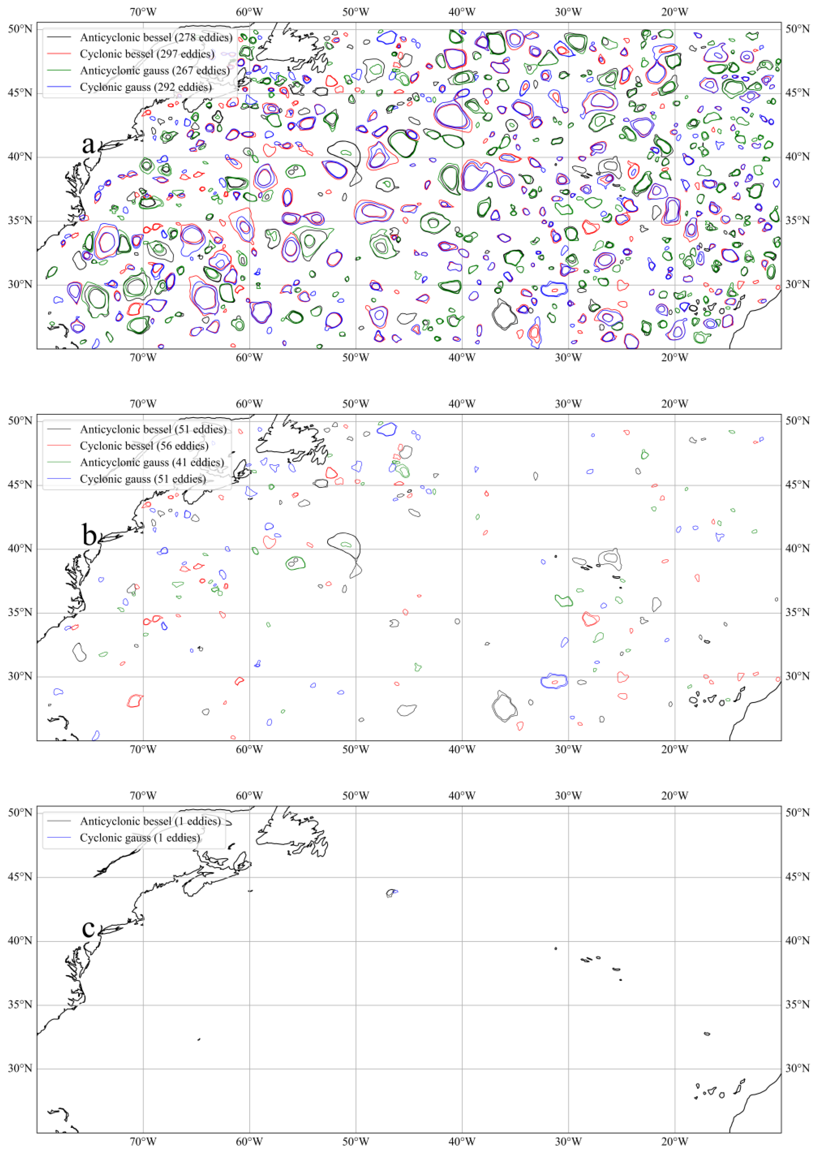
4.1. Single-Day Eddy Characteristics Identified at Different Filter Wavelengths

To mitigate the influence of large-scale dynamic processes on mesoscale eddy identification, it is necessary to filter the ADT. In this study, a Bessel filter was applied to identify mesoscale eddies using ADT filtered at four different filter wavelengths: 800, 600, 400, and 200 km. The spatial scale of mesoscale eddies typically ranges from tens to hundreds of kilometers [41]. According to previous studies [42,43], mesoscale eddies in the NA generally range from 100 km to 800 km. Therefore, choosing 800 km and 200 km as the upper and lower limits can cover the size range of most mesoscale eddies. The four filter wavelengths of 800 km, 600 km, 400 km, and 200 km were selected primarily to cover eddies of different scales and to evaluate the influence of different filter wavelengths on the identification results of eddies. Taking 27 July 2023 as an example, the effects of different filtering processes on eddy identification are compared, with the results shown in Figure 2. In Figure 2, the red dashed curves represent the effective contours of anticyclonic eddies, defined as the outermost closed contours of the eddies. The solid red curves indicate velocity-based closed contours of AE, which correspond to the closed contours with the maximum mean geostrophic velocity. Similarly, the blue dashed and solid curves denote the effective contours and velocity contours of CE, respectively. Based on the ADT, the number of CE identified using high-pass filtering at filter wavelengths of 800, 600, 400, and 200 km is 297, 307, 363, and 585, respectively. The corresponding numbers of AE are 278, 280, 328, and 549. It is evident that the number of identified eddies increases as the filter wavelength decreases, with most of the increase attributed to small-scale eddies. Thus, the choice of filter wavelength strongly influences the identification of mesoscale eddies on the ocean surface.

Table 1. Dynamic Parameters of Mesoscale Eddies in the North Atlantic on 27 July 2023.

Wavelength (km)	Eddy Type	Number	Mean Effective Radius (km)	Mean Rotational Speed (m/s)	Mean Amplitude (cm)
800	CE	297	38	0.18	5
	AE	278	37	0.15	4
600	CE	307	39	0.18	5
	AE	280	37	0.15	4
400	CE	363	38	0.17	5
	AE	328	37	0.15	3
200	CE	585	32	0.13	3
	AE	549	31	0.11	2

presents the mean values of dynamic parameters for surface mesoscale eddies identified on 27 July 2023, including the effective radius, rotation velocity (calculated as the geostrophic velocity at each point within the eddy based on its closed contours, with the maximum value averaged to determine the rotation velocity), and amplitude. Among these, the dynamic parameters of mesoscale eddies identified after 800 km and 600 km high-pass filtering of ADT are largely similar. When the filter wavelength is reduced to 400 km, the dynamic parameters of mesoscale eddies decrease to varying degrees, though the amplitude shows only minor changes. However, when the filter wavelength is reduced to 200 km, the dynamic parameters of mesoscale eddies exhibit pronounced reductions, highlighting the differences in dynamic characteristics of eddies at different scales. This emphasizes the importance of filtering scale in capturing eddy features. It should be noted that this analysis is based on ADT data for a single day, which introduces considerable uncertainty and potential misjudgment. Therefore, it is necessary to track and analyze eddies over a longer period to accurately assess the impact of different filtering scales on mesoscale eddy identification.

4.2. Characteristics of Long-Term Dynamic Parameters at Different Filter Wavelengths

In this study, a total of 117 days, from 27 July 2023 to 20 November 2023, were selected as the research period to analyze the spatiotemporal characteristics of surface mesoscale eddies in the NA and to track the eddies after identification on a daily basis. To improve the accuracy of eddy identification, avoid misjudgments and multiple identifications, and facilitate a comprehensive analysis of all eddies that formed during the study period, this study focuses on eddies with a lifetime of more than 7 days. These eddies exhibit different timescales and energy levels, and have a certain impact on atmospheric and oceanic systems (

Table 2. Number of mesoscale eddies (lifetimes longer than 7 days) in the North Atlantic.

Wavelength (km)	Eddy Type	Number	Percent of Observation
800	CE	28,099	51.2
	AE	26,733	48.8
600	CE	29,386	51.5
	AE	27,643	48.5
400	CE	34,613	51.7
	AE	32,344	48.3
200	CE	57,339	51.1
	AE	54,846	48.9

). The number of CE with a lifetime longer than 7 days is similar to that of AE, which is consistent with the previous research findings [6,44].

Currently, there are two statistical methods for the analysis of mesoscale ocean surface eddies. One method is to count the cumulative number of eddies identified at each time step (here, each time step is one day) throughout the entire observation period. Another method is to statistically analyze the number of eddy trajectories in a given region. In this study, the first method is used to calculate the amplitude, effective radius, and rotation velocity, while the second method is applied to calculate the lifetime of the eddies.

Figure 3 shows the statistical results of various dynamic parameters for cyclonic and anticyclonic eddies within the study period, illustrating the distribution of amplitude, effective radius, rotation velocity, and the ratio of CE to AE at different filter wavelengths as the dynamic parameters change. From Figure 3, it can be seen that the distribution characteristics of the three dynamic parameters are generally consistent, with eddies mainly concentrated in the range of small amplitude (less than 5 cm), small radius (less than 50 km), and low rotation velocity (less than 10 cm/s). As the dynamic parameters increase, the number of eddies decreases rapidly. With decreasing wavelength, the amplitude and rotation velocity distributions show little change, while the radius distribution decreases from 10–150 km to 10–100 km. The distribution trend of the number of CE and AE is similar, with CE dominating in the range of large amplitude (greater than 15 cm), large radius (greater than 100 km), and high rotation velocity (greater than 20 cm/s). The amplitudes of the eddies are concentrated in the range of 2–5 cm at all filter wavelengths, but the amplitude distribution decreases from 2–20 cm to 2–15 cm as the filter wavelength decreases. The concentrated distribution range of the eddy radius decreases rapidly with decreasing filter wavelength, from 800 km to 200 km, with intervals of 10–150 km, 10–100 km, 10–75 km, and 10–50 km, respectively. The maximum radius decreases from 150 km to 100 km, and the concentrated distribution range of eddy rotation speed remains at 0–10 cm/s. However, the maximum rotation speed decreases from 80 cm/s to 60 cm/s.

To obtain more accurate statistics on the lifetime, eddies with a complete life cycle of generation and extinction in the study area are selected for analysis. Figure 4 shows the statistical results of the lifetime of cyclonic and anticyclonic eddies at different filter wavelengths. As seen in the figure, the number of eddies decreases rapidly as the lifetime increases, with most eddies having a short lifetime, typically within 21 days. When the lifetime is shorter than 28 days, the ratio of CE to AE hovers close to 1. However, when the lifetime surpasses 28 days, the ratio exhibits substantial fluctuations, with CE occurring more frequently. Overall, with the decrease in wavelength, the distribution characteristics of the number of eddies with respect to the lifetime are generally consistent.

Taking an AE identified at a filter wavelength of 800 km as an example, Figure 5 shows the relationship between the eddy’s lifetime and its effective radius and amplitude. The lifetime of the eddies is distinguished by color (in days), and the distribution of these eddies as a percentage of the total number of eddies is shown. In Figure 5a, different colors represent eddies with different lifetimes. As the effective radius increases, the percentage of eddies with short lifetimes (e.g., 7–14 days, black) decreases, while the percentage of eddies with long lifetimes (e.g., 80–117 days, orange) increases. This trend is particularly noticeable when the effective radius exceeds 80 km, as longer-lived eddies tend to have larger effective radii. Figure 5b shows the relationship between the amplitude and lifetime of the eddy. As the amplitude increases, the percentage of short-lifetime eddies (black regions) gradually decreases, while the percentage of long-lifetime eddies (orange and red regions) increases. Particularly, when the amplitude exceeds 0.3 cm, the percentage of long-lifetime eddies is much higher than that of short-lifetime eddies. This suggests that eddies with longer lifetimes tend to have larger amplitudes. Specifically, for every 20 km increase in the effective radius of an eddy (e.g., from 40 km to 60 km), the percentage of eddies with a lifetime exceeding 28 days increases by approximately 10–15%. Additionally, for every 0.1 m increase in amplitude, the percentage of eddies with a lifetime greater than 28 days rises by 15–20%. In general, long-lifetime eddies not only have larger effective radii but also exhibit larger amplitudes, reflecting their higher stability and energy. In contrast, short-lifetime eddies tend to be smaller in scale and amplitude, indicating that they are more unstable and transient.

The normalized lifetime of an eddy removes the influence of varying eddy sizes and intensities, enabling the comparison of lifetime characteristics across different eddies on the same scale. This makes it easier to gain an in-depth understanding of the generation, development, and extinction mechanisms of eddies. The normalized lifetime of NA mesoscale eddies is shown in Figure 6, which illustrates the changes in two dynamic parameters (velocity radius and amplitude) of the eddy under the normalized lifetime. The blue line represents the CE, while the orange line represents the AE. The normalized lifetime (ranging from 0 to 1) represents the complete growth, stability, and decay process of the eddy’s lifetime. The radii and amplitudes of the eddies show a consistent trend over the course of their lifetime: they increase rapidly in the early stages, reach a peak in the middle stage, and then gradually decrease, exhibiting a certain symmetry. The radii of both CE and AE show a similar trend in the normalized lifetime range from 0 to 1. Both radii gradually increase at the beginning of the lifetime, reach their maximum values in the middle period, and decrease gradually in the later stages. The overall trend is similar, and the radii of the CE and AE are very close to each other. In particular, during the middle period, the radii are almost identical, both measuring 30 km. The amplitudes of CE are higher than those of anticyclonic eddies throughout the entire lifetime. During the middle period when the amplitudes reach their peaks, the amplitudes of CE are notably higher than those of AE, and the difference between them attains its maximum value. This may reflect the greater intensity of CE.

EKE measures kinetic energy from eddies, indicating their strength and activity level. It is used to assess the active regions of the eddy and the efficiency of energy transport. The EKE of eddies identified with different filtering wavelengths is shown in Figure 7. The distribution of EKE is remarkably similar across different filtering wavelengths. Eddies are densely distributed between 35°N–45°N and 60°W–50°W, with a large amount of eddies exhibiting high EKE. As we move farther from the western coast, both the number of eddies and the EKE values decrease, indicating weaker eddy activity in this region. Combining Figure 1 and Figure 7, it can be observed that in the 35°N–45°N region of the NA, especially near the western boundary current, the quivers are very dense and the color variations are prominent. This indicates the region has pronounced marine front characteristics, suggesting a steep thermohaline gradient and dynamic instability. The dynamic characteristics of the front region enhance the instability of the local flow field, promoting the formation of eddies and thereby increasing local EKE. This indicates a close relationship between the ocean front and the instability of the local flow field, which not only affects the structure of regional ocean dynamics but also has a significant impact on ocean heat and material transport processes.

4.3. Eddy Trajectory Analysis

To further explore the dynamic changes of strong mesoscale eddies in the study area, all eddies with a lifetime of longer than 45 days during the study period were extracted for trajectory analysis. Among them, 81, 77, 90, and 111 CEs were identified at filter wavelengths of 800, 600, 400, and 200 km, respectively, along with 62, 57, 74, and 78 AEs. Figure 8 shows the traces of strong mesoscale eddies identified at a filter wavelength of 800 km. It can be seen that most eddies propagate westward, and the distribution of long-track eddies is concentrated in the NA, where strong circulation and greater EKE are present. These eddies exhibit higher propagation speeds, resulting in longer traces. Strong mesoscale eddies are also found outside the strong current regions of the ocean circulation (45°N–50°N, 10°W–30°W in Figure 8a), but these eddies have smaller EKE, slower propagation speeds, and shorter motion trajectories. As the filter wavelength decreases, long-track eddies remain concentrated in the strong current regions, with no noticeable change in their number, while the amount of short-track eddies increases significantly. The intensity of the trajectories increases overall, indicating that short-lived, small-scale eddies can be effectively detected as the filter wavelength decreases.

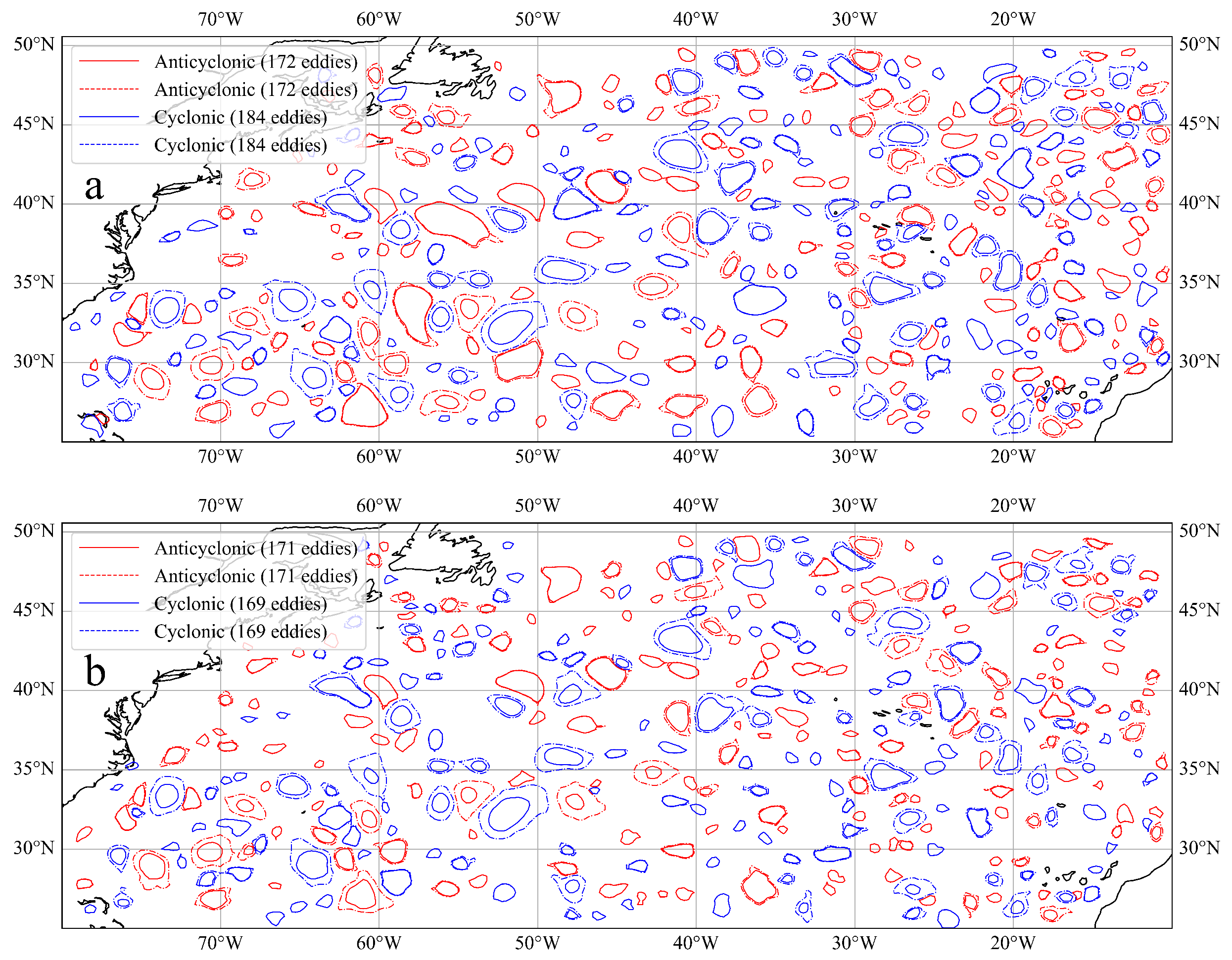
5. Comparison of Eddy Detection from Different Data Sources

Most previous studies rely on multi-year SSH data for eddy analysis [15,45]. However, the limited 117-day time coverage of SWOT data restricts a comprehensive understanding of long-term eddy characteristics. This study takes multi-source satellite altimeter data and the META3.2exp NRT for comparative analysis. These datasets effectively complement the limitations of SWOT data in long-term eddy identification, enhancing result reliability and accuracy through cross-validation. To ensure consistency in spatial resolution between SWOT data and multi-source satellite altimeter data, the SWOT data was resampled to a 1/4° resolution. Both the resampled SWOT data and multi-source satellite altimeter data were processed with the same algorithm, filtering method, and filter wavelengths to detect eddies from the ADT data on 27 July 2023. Figure 9a shows the eddy distribution from multi-source satellite altimeter data, with 172 AEs and 184 CEs. Figure 9b displays the results from the resampled SWOT data, identifying 171 AEs and 169 CEs. The minimal discrepancy in the count of eddies, along with the strikingly similar morphology and spatial distribution exhibited by the two datasets, firmly validates the accuracy of SWOT data when it comes to identifying mesoscale eddies.

Figure 10 illustrates the dynamic parameters of mesoscale eddies identified using different data sources from 27 July 2023 to 20 November 2023. Figure 10a1–a3 show the eddy amplitude, effective radius, and rotation velocity identified from multi-source satellite altimeter data, while Figure 10b1–b3 show the results from SWOT data. To distinguish small-scale eddies, this study defines them as having an amplitude less than 10 cm, an effective radius less than 50 km, or a rotation speed less than 20 cm/s. Otherwise, they are considered large-scale eddies. According to the analysis in Figure 10, 45.0% of CEs identified by multi-source satellite altimeter data have an effective radius smaller than 50 km, and 38.1% meet all three conditions. For AEs, 43.2% of them have an effective radius less than 50 km, and 38.7% meet all three conditions. Among CEs identified by SWOT data, 50.3% of them have an effective radius smaller than 50 km, and 39.7% meet all three conditions. For AEs, 49.6% of them have an effective radius less than 50 km, and 42.9% meet all three conditions. In summary, SWOT data demonstrate clear advantages in identifying small-scale eddies. As SWOT’s time coverage expands, its role in mesoscale eddy identification and related research will become increasingly important.

In this study, the META3.2exp NRT dataset was utilized for comparative experiments, with its input data derived from the near-real-time ADT data of DUACS2018, covering the period from 2018 to 2024. Data processing was conducted using the Lanczos filtering method with a filtering wavelength of 700 km, and mesoscale eddy identification and tracking were performed using the PET algorithm. To ensure the accuracy of the comparative analysis, resampled SWOT data (27 July 2023 to 20 November 2023) were employed to re-identify and re-track mesoscale eddies in the NA using the same filtering method and wavelength. A 7-day time limit was set for the tracking of both datasets, meaning that only eddies with a lifetime longer than 7 days were counted. A comparison of eddy lifetime distributions between the two datasets (Figure 11) revealed a generally similar trend, with most eddies persisting for durations ranging from several days to a few dozen days. However, a notable difference was observed: the peak eddy lifetime in the META3.2exp NRT dataset occurred at 13–15 days, whereas the SWOT dataset exhibited a peak at 7–9 days. This discrepancy may be attributed to differences in the spatial resolution of the satellite altimeters. In summary, despite the relatively short temporal coverage of the SWOT data, its analysis remains valuable for studying mesoscale eddies in the NA, providing meaningful insights into their characteristics and variability.

By integrating multi-source data, this study validates the accuracy of SWOT data in eddy identification and provides a more comprehensive and reliable analysis. A comparison with multi-source satellite altimeter data demonstrates that SWOT data exhibits substantial advantages in capturing the characteristics of small-scale eddies. Despite its limited time span, SWOT data have emerged as a valuable tool in ocean dynamics research due to their high spatial resolution and capability to detect small-scale eddies. With the continuous accumulation of observational data, SWOT data are expected to play an increasingly important role in long-period eddy studies, ocean dynamics research, and climate change investigations.

6. Discussions

6.1. Influence of Different Filters on Eddy Identification

There are two approaches to assessing the effect of different filtering methods on eddy identification: applying the same filter with different filter wavelengths or using two distinct filters. In this study, the Bessel filter was employed. Figure 12 presents the eddy identification results obtained using a Gaussian filter at the same filter wavelength for comparison. Figure 12a illustrates all the eddies identified by both filters, showing dense contours and a wide distribution. Figure 12b highlights eddies with different locations or radii between the two identification results, indicating that while the overall distribution of eddies is similar, slight differences appear in the specific locations and scales of individual eddies. Figure 12c displays encounters between cyclonic and anticyclonic eddies, which may include anomalous or interfering signals, further demonstrating the subtle influence of filter selection on the identification results. After removing these anomalous eddies, 241 CEs and 227 AEs were identified by consensus.The dynamic parameters of the eddies identified by both filters are generally consistent, though some differences exist in specific details, such as the position and size of the eddies. The Bessel filter performs better in terms of boundary smoothness, whereas the Gaussian filter is more sensitive to local perturbations, making it suitable for capturing fine-scale eddy variations. Therefore, when the focus is on macroscopic characteristics of eddies, either filter can be used. However, if smoother boundaries are required or the influence of anomalies needs to be minimized, the Bessel filter may be the preferable choice.

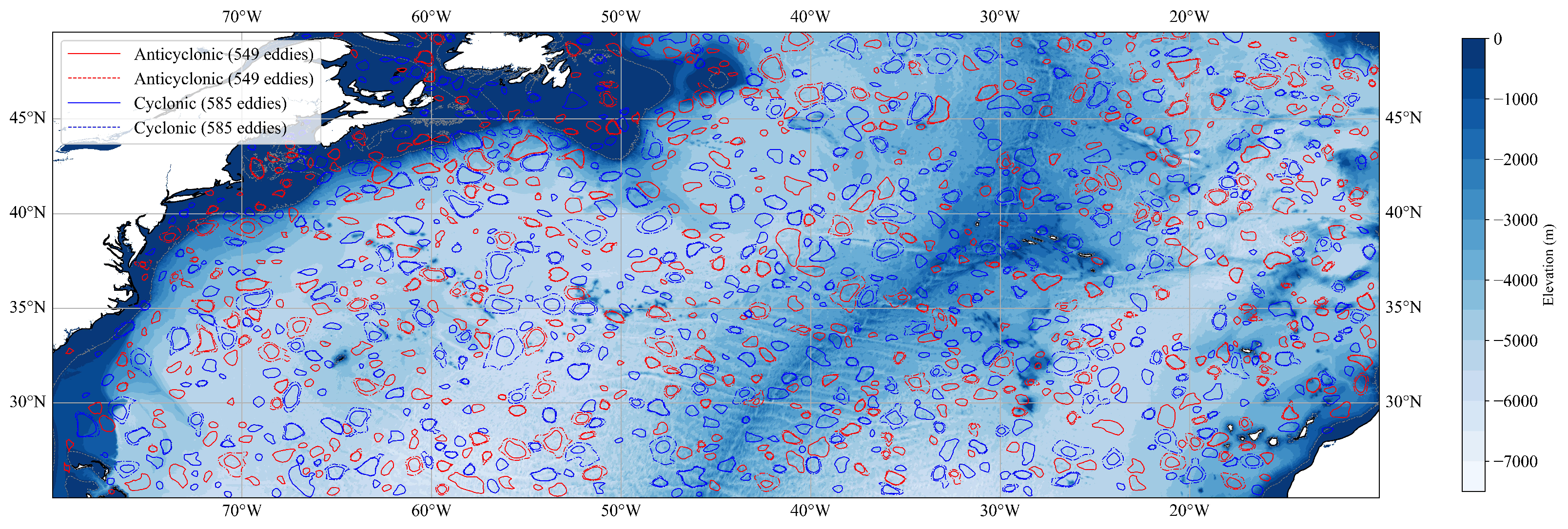
6.2. The Influence of Submarine Topography on Eddy Identification

The closed contour method is sensitive to the geometric features of eddies, and this method identifies eddies based on physical characteristics. As a result, it may be influenced by seamounts or other interference factors in the recognition process. Seamounts are common features in the ocean, with over 14,500 seamounts discovered to date [46,47,48,49,50,51,52]. Since seamounts typically have local bulges and can induce local circulations (such as upwelling), these topographic effects may create characteristics resembling closed contours in the identification results, leading to misidentification of eddies. To explore the influence of seamounts, this study compared the results of mesoscale eddies identified at a 200 km filter wavelength with seabed topography data from GERCO (Figure 13). It was found that the eddies were evenly distributed across the study area. The number and density of eddies did not change substantially in both the raised seamount areas and the flat seabed areas, suggesting that submarine topography has minimal influence on eddy identification. Since the 200 km filter wavelength is longer than the scale of most seamounts, eddy identification is primarily driven by large-scale dynamic processes in the ocean. Even in regions with pronounced topographic variations, the eddy profiles remained intact and were not distorted or influenced by topographic interference. This suggests that submarine topography has a limited impact on eddy identification.

6.3. Limitations and Future Directions

This study reveals the temporal and spatial characteristics of mesoscale eddies through SWOT data analysis over a short time period. However, due to the limited timespan, the results cannot fully capture the long-term evolution of eddies or account for seasonal and interannual variations. Future research should extend the timescale and incorporate long-term datasets to further validate and expand upon these findings.

Mesoscale eddies play a crucial role in ocean circulation, mass transport, the climate system, and energy exchange. By analyzing the temporal and spatial characteristics of NA eddies, this study provides valuable data for understanding the impact of eddies on heat, salt, and nutrient distribution. The identification of eddies using different filter wavelengths offers a more refined perspective on ocean dynamics, which can improve climate model simulations and enhance prediction accuracy. While satellite remote sensing enables large-scale and real-time ocean monitoring, eddy identification still faces challenges related to spatiotemporal scale and accuracy. Future studies could leverage deep learning to advance satellite oceanography [53,54].

7. Conclusions

In this study, the latest SWOT satellite altimeter L4 data are utilized to analyze the spatial and temporal distribution, as well as the dynamic characteristics of mesoscale eddies in the North Atlantic Ocean from 27 July 2023 to 20 November 2023. The analysis is conducted using the PET algorithm based on the ADT closed contour principle. By applying the high-pass filter method, different filter wavelengths are selected to investigate their impact on mesoscale eddy identification, and potential factors influencing this identification are discussed. The main conclusions are as follows:

(1)

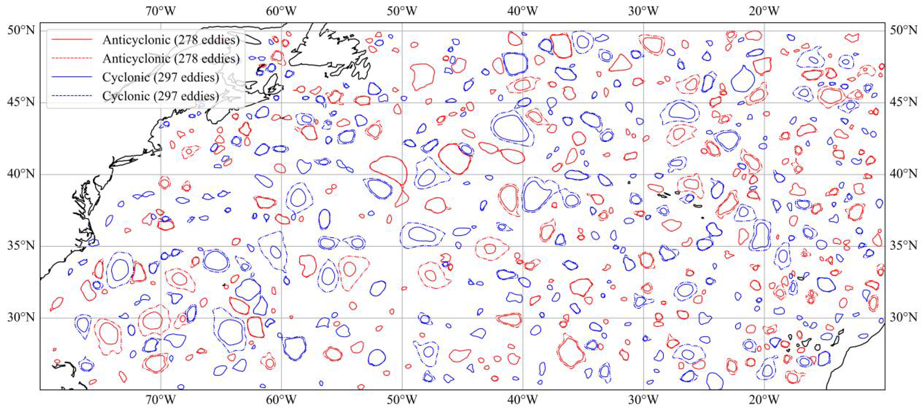
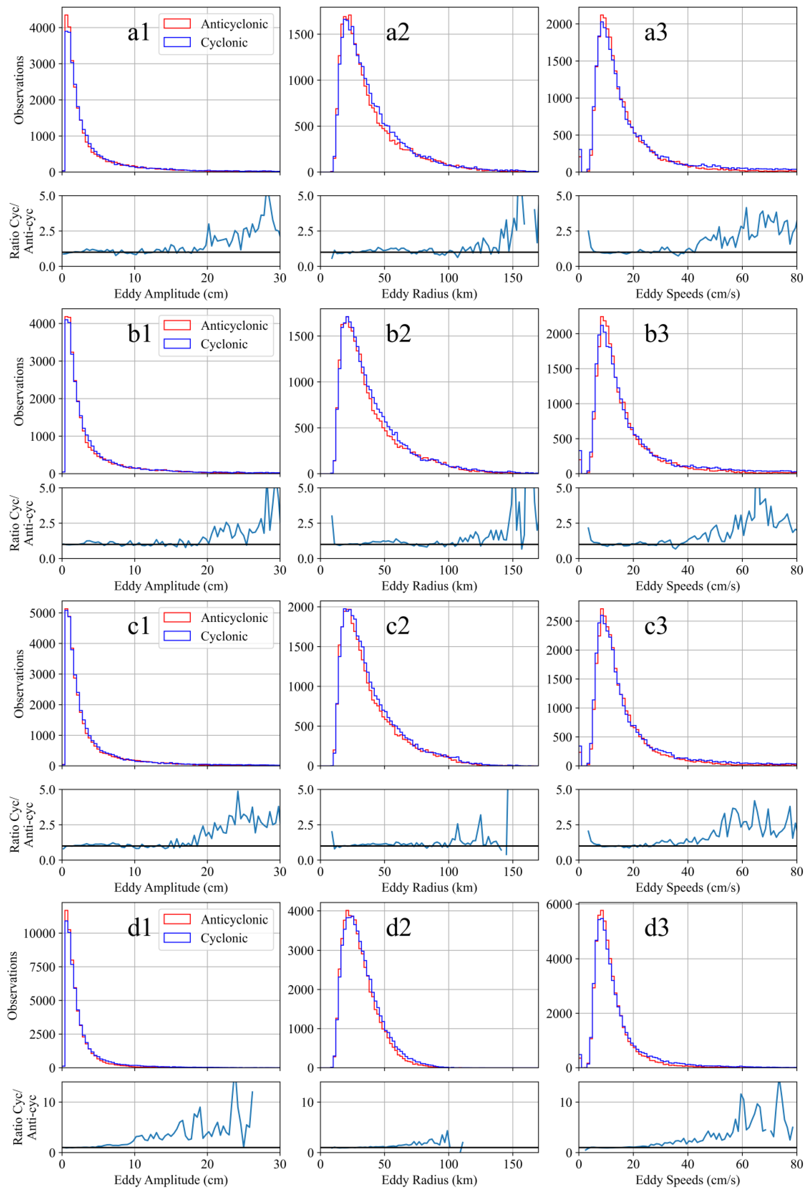
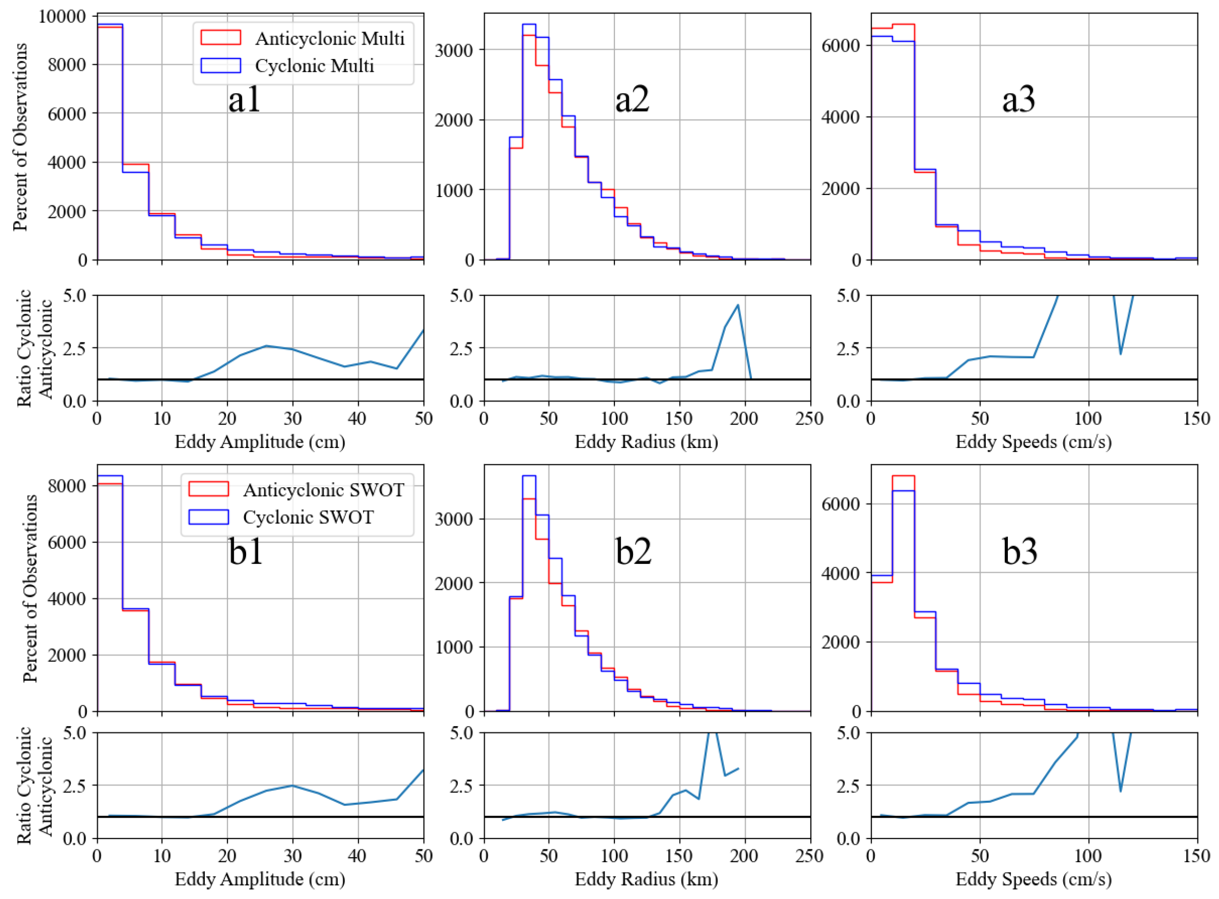
The energy of mesoscale eddies primarily originates from the instabilities of strong boundary currents. As the filter wavelength decreases, the number of identified CE and AE eddies increases; however, the ratio between them consistently remains close to 1.1:1. At different filter wavelengths, the distribution characteristics of the dynamic parameters for cyclonic and anticyclonic eddies are generally similar, predominantly concentrated in the ranges of small amplitude, small radius, and low rotation velocity. With a decrease in filter wavelength, the range of eddy dynamic parameters becomes narrower, and the number of CEs with large amplitude, large radius, and high rotation velocity becomes more prominent. At the same filter wavelength, the dynamic parameters of eddies identified using different filters are broadly consistent, although minor differences in aspects such as position and size can be observed.

(2)

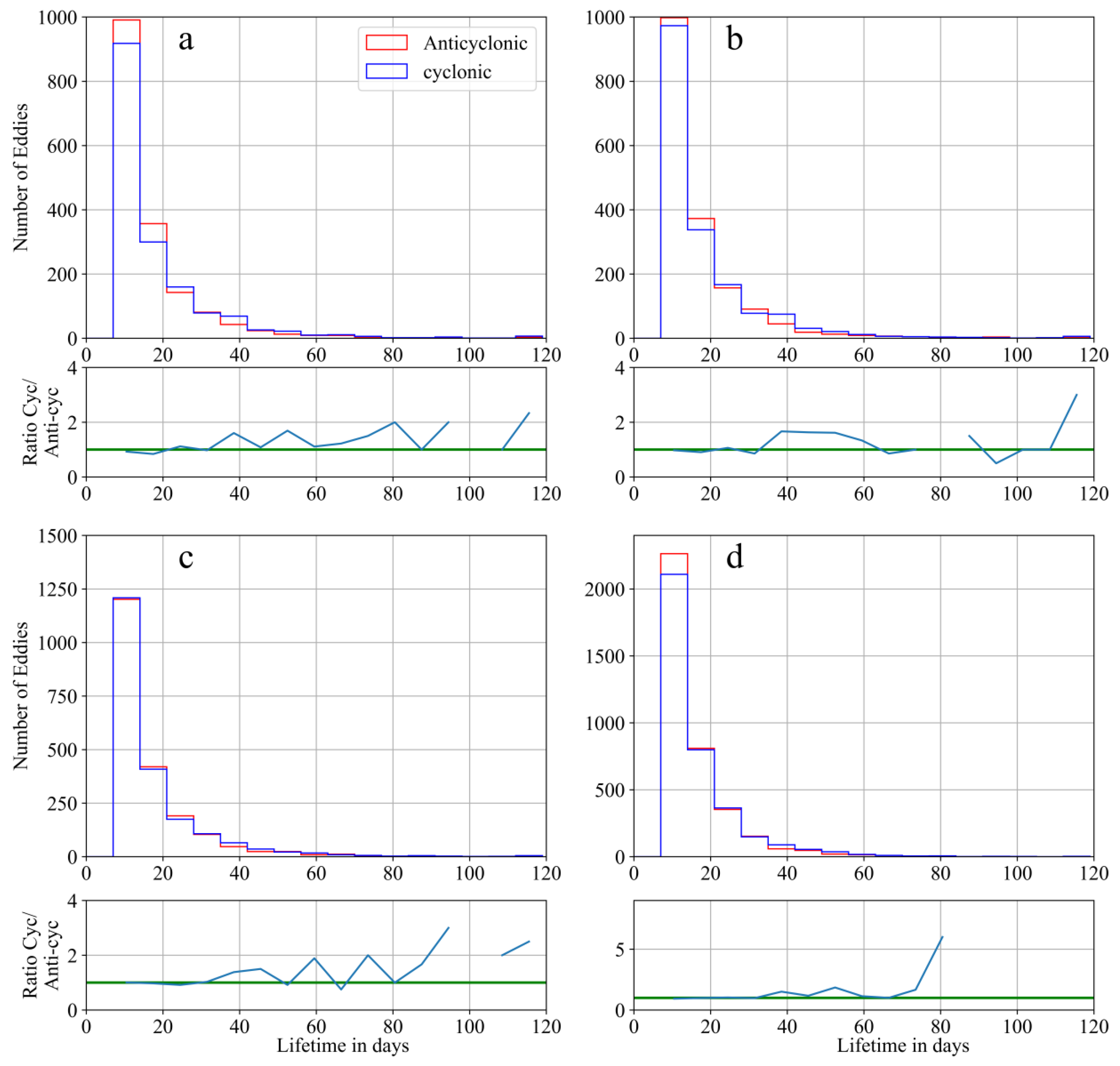
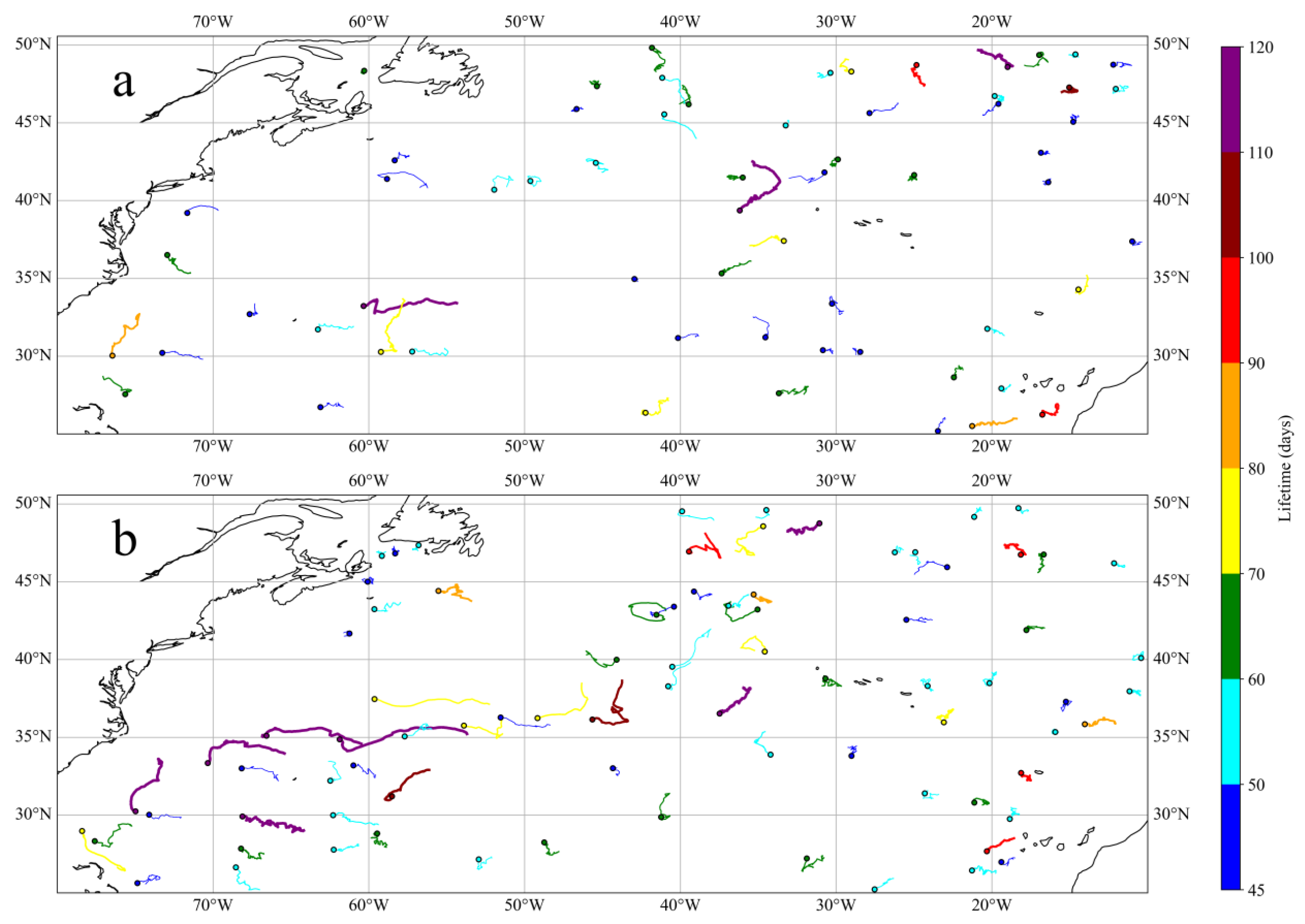
Based on the eddy identification results over a period of 117 days, the majority of mesoscale eddies have lifetimes ranging from 7 to 21 days, with those exhibiting larger amplitudes and effective radii tending to have longer lifetimes. In contrast, smaller eddies generally have shorter lifetimes. Strong mesoscale eddies with lifetimes exceeding 45 days are more likely to form extended trajectories. These long-lived eddies are primarily concentrated in regions of strong circulation and high EKE in the North Atlantic. In comparison, eddies located farther from strong current regions exhibit lower EKE, slower propagation speeds, and shorter trajectories.

(3)

This study confirms the exceptional capability of SWOT data in accurately capturing small- and medium-scale eddies. As SWOT satellite observational data continue to accumulate, its role in elucidating multi-scale ocean dynamic processes will be further enhanced, providing critical support for an in-depth understanding of ocean dynamic mechanisms.

References

1. Feng, S.; Li, F.; Li, S. Introduction to Marine Science; Higher Education Press: Beijing, China, 1999. (In Chinese) [Google Scholar]
2. Beckmann, A.; Böning, C.W.; Brügge, B.; Stammer, D. On the generation and role of eddy variability in the central North Atlantic Ocean. J. Geophys. Res. Ocean. 1994, 99, 20381–20391. [Google Scholar] [CrossRef]
3. Sasaki, H.; Klein, P.; Qiu, B.; Sasai, Y. Impact of oceanic-scale interactions on the seasonal modulation of ocean dynamics by the atmosphere. Nat. Commun. 2014, 5, 5636. [Google Scholar] [CrossRef]
4. Klein, P.; Lapeyre, G.; Siegelman, L.; Qiu, B.; Fu, L.L.; Torres, H.; Su, Z.; Menemenlis, D.; Le Gentil, S. Ocean-scale interactions from space. Earth Space Sci. 2019, 6, 795–817. [Google Scholar] [CrossRef]
5. McGillicuddy, D.J., Jr.; Anderson, L.A.; Bates, N.R.; Bibby, T.; Buesseler, K.O.; Carlson, C.A.; Davis, C.S.; Ewart, C.; Falkowski, P.G.; Goldthwait, S.A.; et al. Eddy/wind interactions stimulate extraordinary mid-ocean plankton blooms. Science 2007, 316, 1021–1026. [Google Scholar] [CrossRef]
6. Chelton, D.B.; Gaube, P.; Schlax, M.G.; Early, J.J.; Samelson, R.M. The Influence of Nonlinear Mesoscale Eddies on Near-Surface Oceanic Chlorophyll. Science 2011, 334, 328–332. [Google Scholar] [CrossRef]
7. Dong, C.; McWilliams, J.C.; Liu, Y.; Chen, D. Global heat and salt transports by eddy movement. Nat. Commun. 2014, 5, 3294. [Google Scholar] [CrossRef]
8. Zhang, Z.; Wang, W.; Qiu, B. Oceanic mass transport by mesoscale eddies. Science 2014, 345, 322–324. [Google Scholar] [CrossRef] [PubMed]
9. Zhang, Z.; Tian, J.; Qiu, B.; Zhao, W.; Chang, P.; Wu, D.; Wan, X. Observed 3D structure, generation, and dissipation of oceanic mesoscale eddies in the South China Sea. Sci. Rep. 2016, 6, 24349. [Google Scholar] [CrossRef]
10. Fu, L.L.; Alsdorf, D.; Morrow, R.; Rodriguez, E.; Mognard, N. SWOT: The Surface Water and Ocean Topography Mission. Wide-Swath Altimetric Elevation on Earth; Technical Report; NASA Jet Propulsion Laboratory: Pasadena, CA, USA, 2012.
11. Stammer, D. Global characteristics of ocean variability estimated from regional TOPEX/POSEIDON altimeter measurements. J. Phys. Oceanogr. 1997, 27, 1743–1769. [Google Scholar] [CrossRef]
12. Brokaw, R.J.; Subrahmanyam, B.; Trott, C.B.; Chaigneau, A. Eddy surface characteristics and vertical structure in the Gulf of Mexico from satellite observations and model simulations. J. Geophys. Res. Ocean. 2020, 125, e2019JC015538. [Google Scholar] [CrossRef]
13. Zhu, Y.; Liang, X. Characteristics of Eulerian mesoscale eddies in the Gulf of Mexico. Front. Mar. Sci. 2022, 9, 1087060. [Google Scholar] [CrossRef]
14. Zhang, Y.; Hu, C.; McGillicuddy, D.J., Jr.; Liu, Y.; Barnes, B.B.; Kourafalou, V.H. Mesoscale eddies in the Gulf of Mexico: A three-dimensional characterization based on global HYCOM. Deep. Sea Res. Part II Top. Stud. Oceanogr. 2024, 215, 105380. [Google Scholar] [CrossRef]
15. Aguedjou, H.; Dadou, I.; Chaigneau, A.; Morel, Y.; Alory, G. Eddies in the Tropical Atlantic Ocean and their seasonal variability. Geophys. Res. Lett. 2019, 46, 12156–12164. [Google Scholar] [CrossRef]
16. Ioannou, A.; Speich, S.; Laxenaire, R. Characterizing mesoscale eddies of eastern upwelling origins in the Atlantic Ocean and their role in offshore transport. Front. Mar. Sci. 2022, 9, 835260. [Google Scholar] [CrossRef]
17. Kang, D.; Curchitser, E.N. Gulf Stream eddy characteristics in a high-resolution ocean model. J. Geophys. Res. Ocean. 2013, 118, 4474–4487. [Google Scholar] [CrossRef]
18. Waseda, T.; Mitsudera, H.; Taguchi, B.; Yoshikawa, Y. On the eddy-Kuroshio interaction: Evolution of the mesoscale eddy. J. Geophys. Res. Ocean. 2002, 107, 3-1–3-9. [Google Scholar] [CrossRef]
19. Abdalla, S.; Kolahchi, A.A.; Ablain, M.; Adusumilli, S.; Bhowmick, S.A.; Alou-Font, E.; Amarouche, L.; Andersen, O.B.; Antich, H.; Aouf, L.; et al. Altimetry for the future: Building on 25 years of progress. Adv. Space Res. 2021, 68, 319–363. [Google Scholar] [CrossRef]
20. Woodworth, P.L.; Menéndez, M. Changes in the mesoscale variability and in extreme sea levels over two decades as observed by satellite altimetry. J. Geophys. Res. Ocean. 2015, 120, 64–77. [Google Scholar] [CrossRef]
21. Yu, Y.; Sandwell, D.; Gille, S. Seasonality of the sub-mesoscale to mesoscale Sea Surface variability from multi-year satellite altimetry. J. Geophys. Res. Ocean. 2023, 128, e2022JC019486. [Google Scholar] [CrossRef]
22. Stammer, D.; Böning, C.W. Generation and distribution of mesoscale eddies in the North Atlantic Ocean. In The Warm Watersphere of the North Atlantic Ocean; Bornträger: Berlin, Germany, 1996. [Google Scholar]
23. Stammer, D.; Wunsch, C. Temporal changes in eddy energy of the oceans. Deep. Sea Res. Part II Top. Stud. Oceanogr. 1999, 46, 77–108. [Google Scholar] [CrossRef]
24. Brachet, S.; Le Traon, P.Y.; Le Provost, C. Mesoscale variability from a high-resolution model and from altimeter data in the North Atlantic Ocean. J. Geophys. Res. Ocean. 2004, 109. [Google Scholar] [CrossRef]
25. Qiu, B.; Nakano, T.; Chen, S.; Klein, P. Bi-directional energy cascades in the Pacific Ocean from equator to subarctic gyre. Geophys. Res. Lett. 2022, 49, e2022GL097713. [Google Scholar] [CrossRef]
26. Zhang, Z.; Liu, Y.; Qiu, B.; Luo, Y.; Cai, W.; Yuan, Q.; Liu, Y.; Zhang, H.; Liu, H.; Miao, M.; et al. Submesoscale inverse energy cascade enhances Southern Ocean eddy heat transport. Nat. Commun. 2023, 14, 1335. [Google Scholar] [CrossRef] [PubMed]
27. Zhang, Z.; Miao, M.; Qiu, B.; Tian, J.; Jing, Z.; Chen, G.; Chen, Z.; Zhao, W. Submesoscale eddies detected by SWOT and moored observations in the Northwestern Pacific. Geophys. Res. Lett. 2024, 51, e2024GL110000. [Google Scholar] [CrossRef]
28. Fu, L.L.; Ubelmann, C. On the transition from profile altimeter to swath altimeter for observing global ocean surface topography. J. Atmos. Ocean. Technol. 2014, 31, 560–568. [Google Scholar] [CrossRef]
29. Tchonang, B.C.; Benkiran, M.; Le Traon, P.Y.; Jan van Gennip, S.; Lellouche, J.M.; Ruggiero, G. Assessing the impact of the assimilation of swot observations in a global high-resolution analysis and forecasting system–part 2: Results. Front. Mar. Sci. 2021, 8, 687414. [Google Scholar] [CrossRef]
30. Fu, L.L.; Pavelsky, T.; Cretaux, J.F.; Morrow, R.; Farrar, J.T.; Vaze, P.; Sengenes, P.; Vinogradova-Shiffer, N.; Sylvestre-Baron, A.; Picot, N.; et al. The surface water and ocean topography mission: A breakthrough in radar remote sensing of the ocean and land surface water. Geophys. Res. Lett. 2024, 51, e2023GL107652. [Google Scholar] [CrossRef]
31. Chester, D.; Malanotte-Rizzoli, P.; Lynch, J.; Wunsch, C. The eddy radiation field of the Gulf Stream as measured by ocean acoustic tomography. Geophys. Res. Lett. 1994, 21, 181–184. [Google Scholar] [CrossRef]
32. Stommel, H. The Gulf Stream: A Physical and Dynamical Description; University of California Press: Berkeley, CA, USA, 2023. [Google Scholar]
33. Fofonoff, N. The Gulf Stream. In Evolution of Physical Oceanography: Scientific Surveys in Honor of Henry Stommel; MIT Press: Cambridge, MA, USA, 1981; pp. 112–139. [Google Scholar]
34. Rossby, T. The North Atlantic Current and surrounding waters: At the crossroads. Rev. Geophys. 1996, 34, 463–481. [Google Scholar] [CrossRef]
35. Mason, E.; Pascual, A.; McWilliams, J.C. A new sea surface height–based code for oceanic mesoscale eddy tracking. J. Atmos. Ocean. Technol. 2014, 31, 1181–1188. [Google Scholar] [CrossRef]
36. Yongchui, Z.; Ning, W.; Lin, Z.; Kefeng, L.; Haodi, W. The surface and three-dimensional characteristics of mesoscale eddies: A review. Adv. Earth Sci. 2020, 35, 568. [Google Scholar]
37. Chaigneau, A.; Gizolme, A.; Grados, C. Mesoscale eddies off Peru in altimeter records: Identification algorithms and eddy spatio-temporal patterns. Prog. Oceanogr. 2008, 79, 106–119. [Google Scholar] [CrossRef]
38. Chaigneau, A.; Eldin, G.; Dewitte, B. Eddy activity in the four major upwelling systems from satellite altimetry (1992–2007). Prog. Oceanogr. 2009, 83, 117–123. [Google Scholar] [CrossRef]
39. Meng, W.; Yanwei, Z.; Zhifei, L.; Jiawang, W. Temporal and spatial characteristics of mesoscale eddies in the northern South China Sea: Statistics analysis based on altimeter data. Adv. Earth Sci. 2019, 34, 1069. [Google Scholar]
40. Sorrentino, R. Electronic Filter Simulation & Design; McGraw-Hill Professional: New York, NY, USA, 2007. [Google Scholar]
41. Robinson, A.R. Eddies in Marine Science; Springer Science & Business Media: Berlin/Heidelberg, Germany, 2012. [Google Scholar]
42. Le Traon, P.Y.; Rouquet, M.C.; Boissier, C. Spatial scales of mesoscale variability in the North Atlantic as deduced from Geosat data. J. Geophys. Res. Ocean. 1990, 95, 20267–20285. [Google Scholar] [CrossRef]
43. Jacobs, G.; Barron, C.; Rhodes, R. Mesoscale characteristics. J. Geophys. Res. Ocean. 2001, 106, 19581–19595. [Google Scholar] [CrossRef]
44. Faghmous, J.H.; Frenger, I.; Yao, Y.; Warmka, R.; Lindell, A.; Kumar, V. A daily global mesoscale ocean eddy dataset from satellite altimetry. Sci. Data 2015, 2, 1–16. [Google Scholar] [CrossRef]
45. Dong, C.; Liu, L.; Nencioli, F.; Bethel, B.J.; Liu, Y.; Xu, G.; Ma, J.; Ji, J.; Sun, W.; Shan, H.; et al. The near-global ocean mesoscale eddy atmospheric-oceanic-biological interaction observational dataset. Sci. Data 2022, 9, 436. [Google Scholar] [CrossRef]
46. Roden, G.I. Effect of seamounts and seamount chains on ocean circulation and thermohaline structure. Seamounts, Isl. Atolls 1987, 43, 335–354. [Google Scholar]
47. Lavelle, J.W.; Mohn, C. Motion, commotion, and biophysical connections at deep ocean seamounts. Oceanography 2010, 23, 90–103. [Google Scholar] [CrossRef]
48. White, M.; Bashmachnikov, I.; Aristegui, J.; Martins, A.; Pitcher, T.; Morato, T.; Hart, P.; Clark, M.; Haggan, N.; Santos, R. Physical processes and seamount productivity In Seamounts: Ecology, Fisheries and Conservation; Wiley: Hoboken, NJ, USA, 2007; pp. 65–84. [Google Scholar]
49. Hillier, J.; Watts, A. Global distribution of seamounts from ship-track bathymetry data. Geophys. Res. Lett. 2007, 34. [Google Scholar] [CrossRef]
50. Wessel, P.; Sandwell, D.T.; Kim, S.S. The global seamount census. Oceanography 2010, 23, 24–33. [Google Scholar] [CrossRef]
51. Yesson, C.; Clark, M.R.; Taylor, M.L.; Rogers, A.D. The global distribution of seamounts based on 30 arc seconds bathymetry data. Deep. Sea Res. Part I Oceanogr. Res. Pap. 2011, 58, 442–453. [Google Scholar] [CrossRef]
52. Watts, A. Science, seamounts and society. Geoscientist 2019, 290, 10–16. [Google Scholar]
53. Martin, S.; Manucharyan, G.E.; Klein, P. New Estimation of Global Mesoscale Surface Currents with Enhanced Resolution Through a Deep Learning Synthesis of Satellite Observations. In Proceedings of the 2024 Ocean Sciences Meeting, AGU, New Orleans, LA, USA, 18–23 February 2024. [Google Scholar]
54. Martin, S.A.; Manucharyan, G.E.; Klein, P. Deep learning improves global satellite observations of ocean eddy dynamics. Geophys. Res. Lett. 2024, 51, e2024GL110059. [Google Scholar] [CrossRef]
Figure 1. Study area. (a) represents the absolute dynamic topography(ADT) of the global ocean surface on 27 July 2023. (b) shows the flow field over the selected region within box (a). The color shading represents the ADT, and the quivers indicate the geostrophic flow velocity, which is calculated based on the filtered ADT. For the calculation method, refer to Section 3.4.
Remotesensing 17 01469 g001
Figure 2. Recognition results at 800 km filter wavelength on 27 July 2023. Solid red curves and dashed curves represent AE, solid blue curves and dashed curves represent CE. The dashed lines indicate the effective contours of the eddies, corresponding to the outermost closed contours of the eddies. The solid line represents the closed contour of the eddy based on velocity, specifically the closed contour that encompasses the maximum mean geostrophic velocity of the eddy.
Remotesensing 17 01469 g002
Figure 3. Identification of mesoscale eddy dynamic parameters at different filter wavelengths. Row from top to bottom (ad) represents the eddy dynamical parameters (amplitude, radius and rotation speed, column from 1 to 3) identified at different filtering radii (800 km, 600 km, 400 km, and 200 km). The subchart below each chart shows the quantity ratio of AEs (red curves) to CEs (blue curves).
Remotesensing 17 01469 g003
Figure 4. Lifetime of eddies identified at different filter wavelengths. (ad) represent the lifetime statistics of eddies identified at filter wavelengths of 800, 600, 400, and 200 km, respectively. The subchart below each chart shows the quantity ratio of AEs (red curves) to CEs (blue curves).The green line indicates the equality of AEs and CEs.
Remotesensing 17 01469 g004
Figure 5. The relationship among lifetime, radius, and amplitude of eddies from 27 July 2023 to 20 November 2023. Lifetime versus radius (a) and amplitude (b). The legend represents the eddies with different lifetimes.
Remotesensing 17 01469 g005
Figure 6. Normalized lifetime characteristics of eddies identified with filter wavelength of 800 km. The statistical distribution of eddies radius (a) and amplitude (b) relative to the normalized lifetime from 27 July 2023 to 20 November 2023, with orange lines for CEs and blue lines for AEs.
Remotesensing 17 01469 g006
Figure 7. EKE of the eddies identified based the ADT on 27 July 2023. (ad) represent the EKE of eddies identified at filter wavelengths of 800, 600, 400, and 200 km, respectively. The color bar represents EKE in cm2/s2. The dashed lines indicate the effective contours of the eddies. The solid line represents the closed contour of the eddy based on velocity.
Remotesensing 17 01469 g007
Figure 8. Eddy trajectories of eddies with lifetime longer than 45 days. (a) represents AEs and (b) represents CEs. The color represents the lifetime of an eddy.
Remotesensing 17 01469 g008
Figure 9. Comparison of eddies on 27 July 2023, identified using multi-source satellite altimeter data (a) and resampled SWOT data (b). The dashed lines indicate the effective contours of the eddies. The solid line represents the closed contour of the eddy based on velocity.
Remotesensing 17 01469 g009
Figure 10. Dynamic parameters (amplitude, radius and rotation speed) of mesoscale eddies identified from multi-source (a1a3) and SWOT data (b1b3). The subchart below each chart shows the quantity ratio of AEs (red curves) to CEs (blue curves).The black line indicates the equality of AEs and CEs.
Remotesensing 17 01469 g010
Figure 11. The lifetime distribution of eddies from META3.2exp NRT data (2018–2024) (a) and results identified from resampled SWOT data during 27 July to 20 November 2023 (b). The subchart below each chart shows the quantity ratio of AEs (red curves) to CEs (blue curves).The green line indicates the equality of AEs and CEs.
Remotesensing 17 01469 g011
Figure 12. Comparison of eddies identified using Gaussian and Bessel filtered ADT. (a) shows the eddies identified by both filters, (b) shows the differences in the eddies identified by the two filters, and (c) shows the AEs and CEs occurring at the same location identified by both filters. The black and red curves represent eddies identified using the Bessel filter, while the green and blue curves represent those identified using the Gaussian filter.
Remotesensing 17 01469 g012
Figure 13. Spatial distribution of eddy identification results on 27 July 2023 and seabed topography. The dashed lines indicate the effective contours of the eddies. The solid line represents the closed contour of the eddy based on velocity.The color map shows the seabed topography.
Remotesensing 17 01469 g013