Abstract
The classification of freshwater ecosystems is essential for effective biodiversity conservation and ecosystem management, particularly with increasing threats. We developed an automated approach to mapping and classifying freshwater ecosystem functional groups based on the IUCN Global Ecosystem Typology (GET), offering a scalable, dynamic and efficient alternative to current manual methods. Our method leveraged remote sensing data and thresholding algorithms to classify ecosystems into distinct ecosystem functional groups, accounting for challenges such as the temporal and spatial complexities of dynamic freshwater ecosystems and inconsistencies in manual classification. Unlike traditional approaches, which rely on manual cross-referencing to adapt existing maps and contain subjective biases, our system is repeatable, transparent and adaptable to new incoming satellite data. We demonstrate the applicability of this method in the Paroo–Warrego region of Australia (~14,000,000 ha), highlighting the automated classification’s capacity to process large areas with diverse ecosystems. Although some functional groups require static datasets due to current limitations in satellite data, the overall approach had high accuracy (84%). This work provides a foundation for future applications to other freshwater ecosystems around the world, underpinning biodiversity management, monitoring and reporting worldwide.
1. Introduction
Understanding, managing and conserving the world’s ecosystems is increasingly important given the climbing biodiversity loss occurring in the Anthropocene, and nearly every country in the world has agreed to halt this loss by 2030 [1,2]. Conserving and sustainably managing freshwater ecosystems are significant environmental challenges given their importance for biodiversity and provision of ecosystem services [3,4,5]. Despite this importance, their degradation continues, with human drivers including rising human populations, water resource development, climate change and urbanization [6,7]. Data-led management and conservation planning of these scarce resources is critical but depends on the availability of accurate high-resolution maps.
Defining the types and extent of freshwater ecosystems is still difficult [8,9], complicated by high temporal and spatial dynamism [10,11]. Approaches vary from on-ground sampling surveying ecosystem features (e.g., water quality, extent, seasonality) [12] to leveraging remote sensing techniques and platforms for scalable mapping, including the use of drones and satellites [8,10]. Global mapping products exist, but they primarily map the extent of surface water [13] without distinguishing the functionally different freshwater ecosystems [14].
Currently, many nations do not have comprehensive ecosystem maps. For those that do, freshwater ecosystem classifications vary among schemes and within and among countries, with different management authorities often employing distinct techniques [15]. This makes comparisons of freshwater ecosystems across borders difficult and inconsistent, and it also makes analyses of large-scale global trends and estimations problematic [16,17]. Transboundary rivers, lakes and floodplains exemplify this problem, with international politics and national self-interest often dictating the level of effort of mapping and conservation [18]. Current IUCN GET maps represent a simple, temporally static, low-resolution conversion of these available inconsistent local or national maps [14]. As such, environmental change cannot be readily captured, limiting responses to rapidly shifting ecosystems [19]. Scalable and repeatable classification methods, transcending political boundaries, are essential for reporting on ecosystem extent and condition. These would allow rigorous spatial and temporal comparisons, including reporting on progress towards 2030 global biodiversity targets, set by the Convention on Biological Diversity [2].
The IUCN Global Ecosystem Typology (IUCN GET) provides a hierarchical approach to classify ecosystems, driven by their functionality [14]. It can provide an agreed reference classification, allowing standardized cross-jurisdictional classifications, and it now underpins the System of Environmental Economic Accounting (SEEA) Ecosystem Accounts and guides the Red List of Ecosystem assessments [1]. For nations to contribute effectively to monitoring and reporting on global biodiversity targets, ecosystem mapping needs to rigorously implement this global approach. Within the freshwater (e.g., rivers and lakes) and related transitional realms (e.g., palustrine and estuarine wetlands), there are currently 39 mutually exclusive ecosystem functional groups [14]. The IUCN Global Ecosystem Typology enforces consistency among the units of ecosystems independently derived from other classifications from local to global scales, with conceptual models guiding choices of key indicators and ecosystem processes, useful for management of threats for groups of functionally related ecosystem types [14]. The IUCN GET conceptual framework provides opportunities to develop systematic and automated tools to drive classifications of functional groups at scale. Such approaches need to be repeatable, rigorous and applicable in regions with high hydrological variability and little available information.
We aimed to develop an automated and repeatable approach for identifying, mapping and classifying freshwater ecosystem functional groups according to the IUCN Global Ecosystem Typology. We used a large region of arid and semi-arid Australia, where there is high variability in the extent and distribution of freshwater flows and diverse freshwater ecosystem types. This encompassed two river basins, crossing state boundaries, where significant anthropogenic impacts affecting freshwater ecosystems have been largely absent [19,20], making these river basins useful for tracking and classifying natural variability of freshwater ecosystems. We aimed to produce a mapping approach which was script-based, temporally dynamic, scalable and consistent across jurisdictional boundaries as a pilot for application across other regions of the world.
2. Materials and Methods
2.1. Study Area
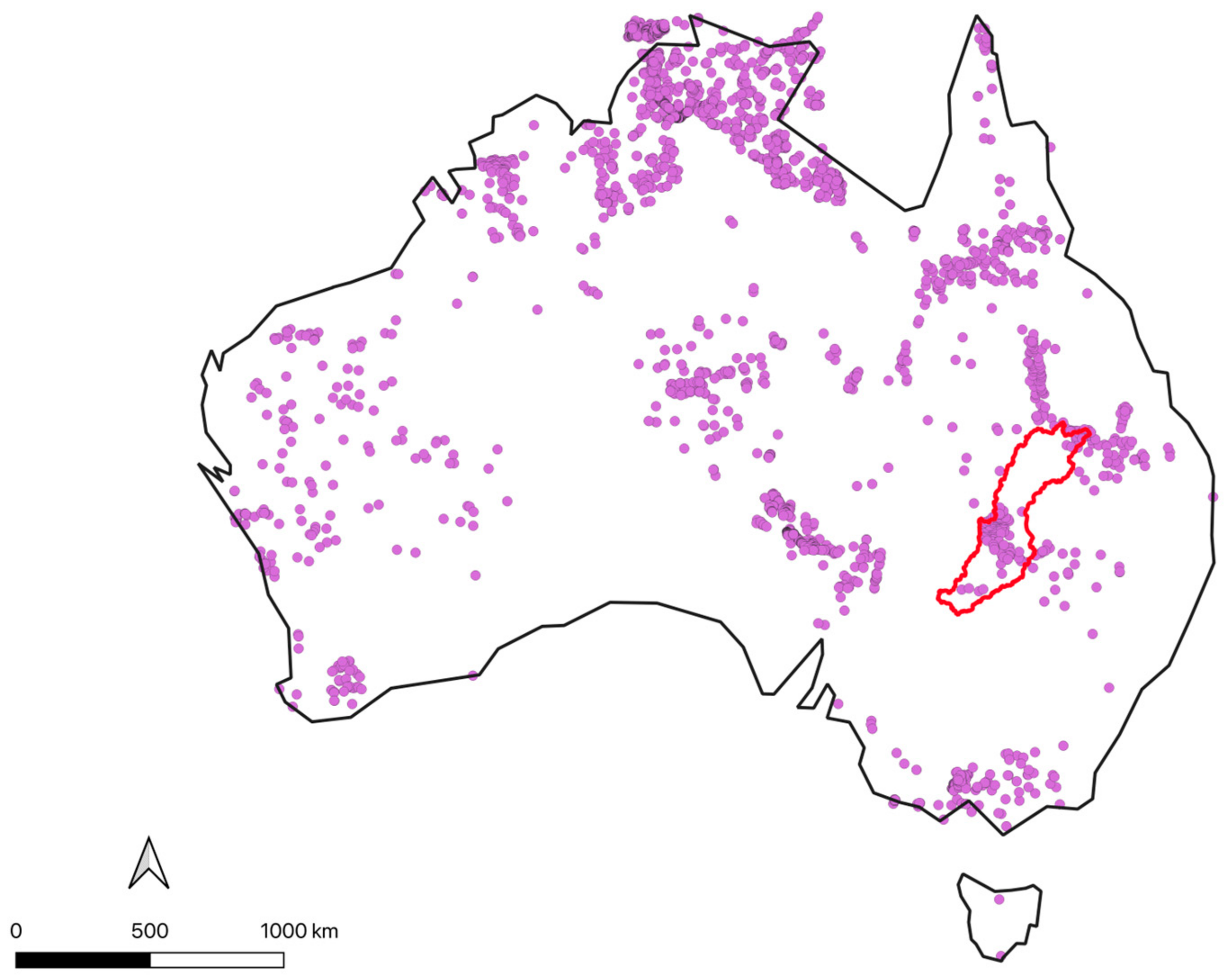
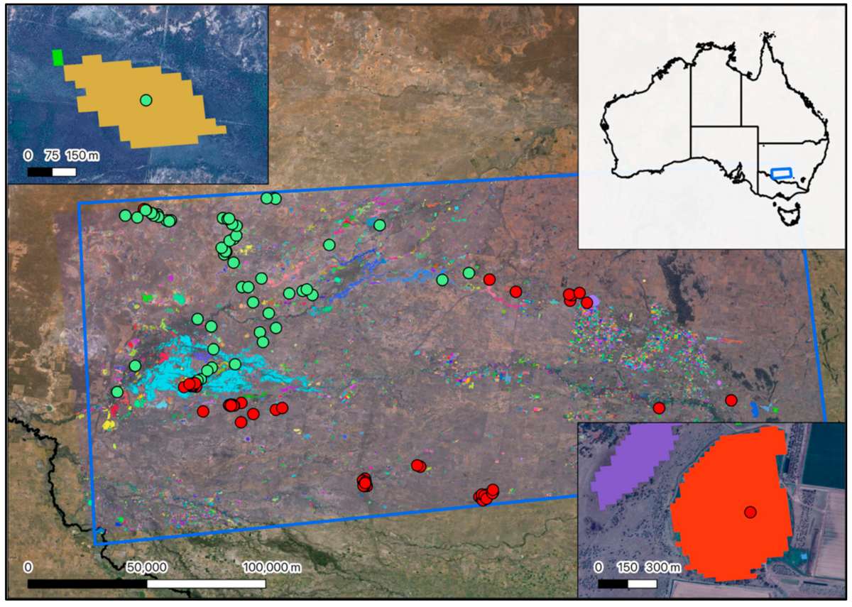
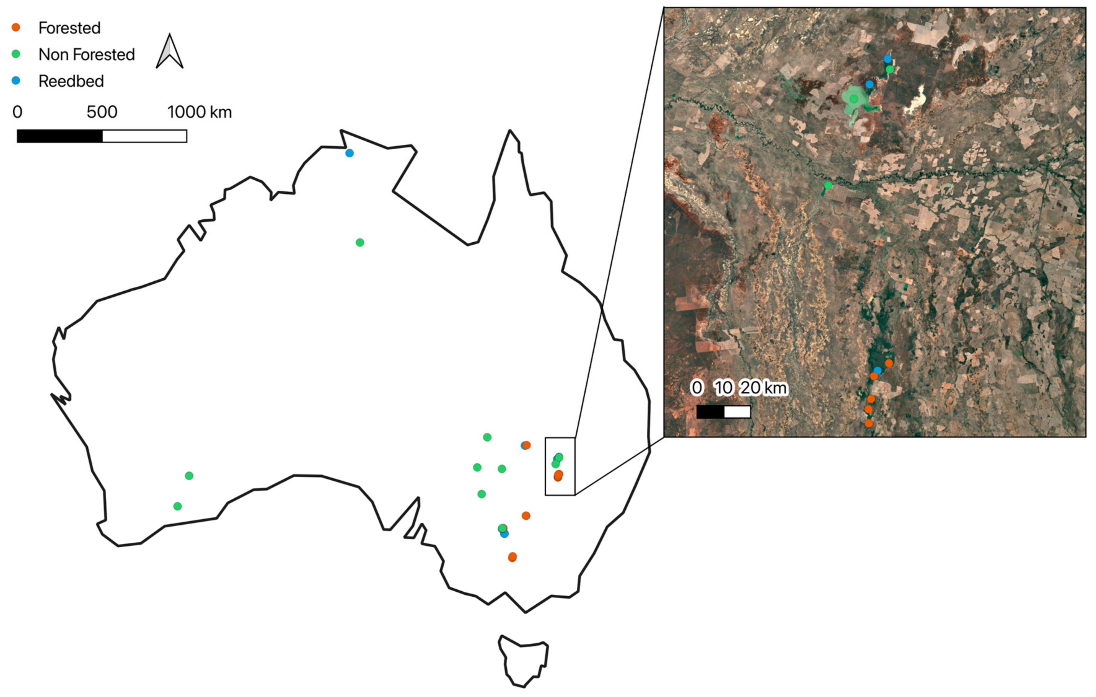
The Paroo and Warrego River systems (hereafter, the Paroo–Warrego), the main focus of this study, are part of the Darling River basin (Figure 1), crossing two states (New South Wales, Queensland), and covering 13,689,186 ha of arid and semi-arid Australia. The catchment receives a median annual precipitation of ~264 mm (131 years of complete data, Wanaaring Post Office Station no. 48079) [21]. The two main rivers, the Paroo and Warrego Rivers, inundated up to ~1,000,000 ha and ~900,000 ha, respectively, of freshwater ecosystems during a significant flood event from flows running off the Chesterton, Warrego, Willies and Walters Ranges (1984–1993) [11,20]. Freshwater ecosystems include rivers, floodplains, different sized temporary and permanent small and large freshwater and saltwater lakes and artesian springs [11]. The greatest extent of freshwater ecosystems was mapped and classified using Landsat satellite imagery, over a period of 10 years (1984–1993) [11], utilized by the Australian National Aquatic Ecosystem Classification [22]. Source data for the study and training data have been collected across the entire Australian continent (see Appendix A, Appendix B, Appendix C, Appendix D, Appendix E, Appendix F, Appendix G, Appendix H, Appendix I, Appendix J and Appendix K for details).
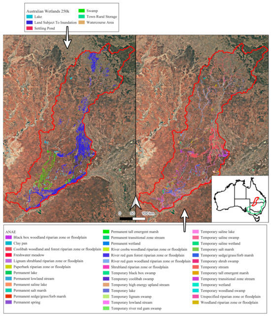
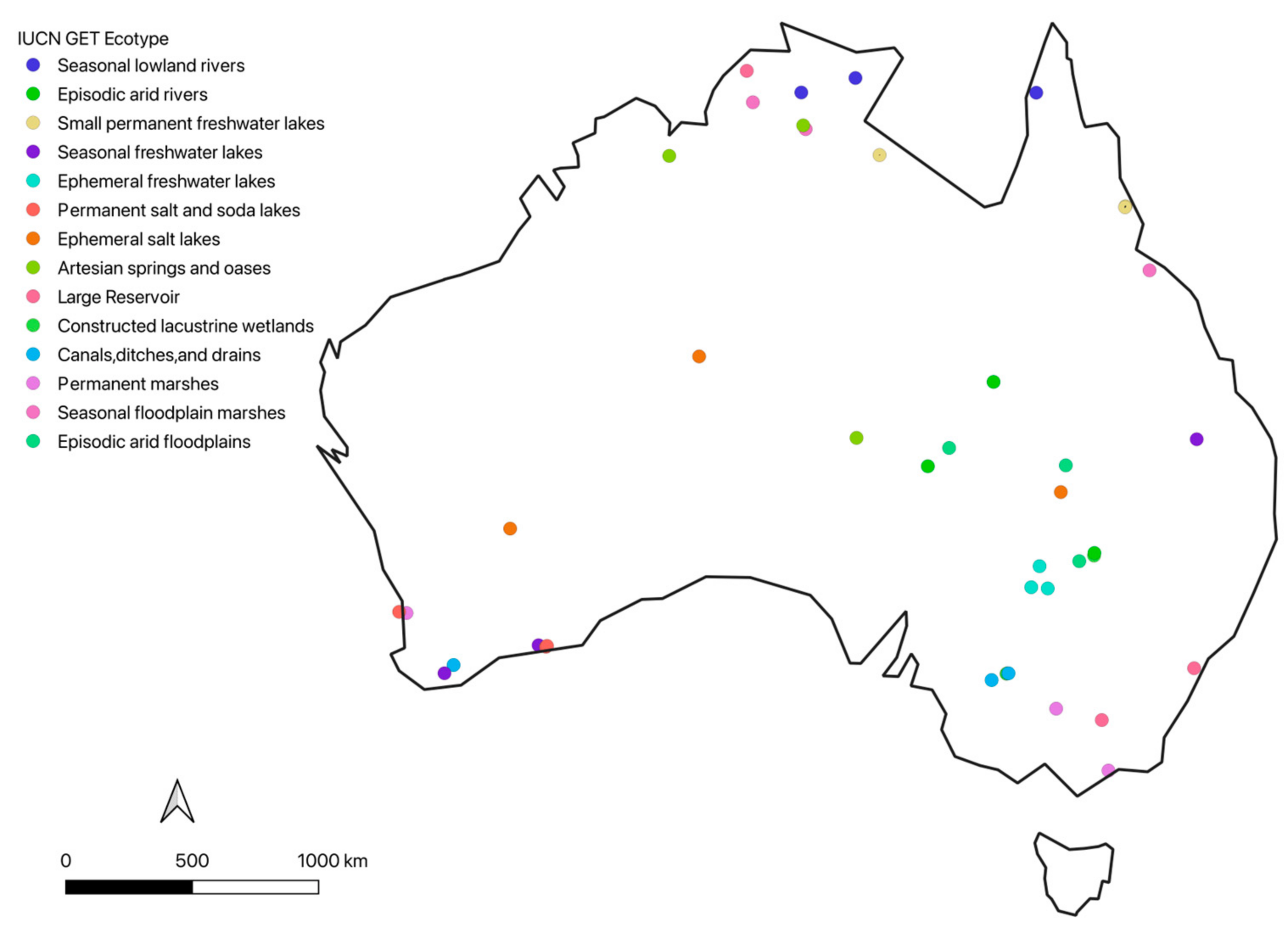
Figure 1.
The Paroo–Warrego River systems in dryland Australia, in the Murray–Darling Basin (green, inset), where we developed automated freshwater ecosystem mapping across a large range of different freshwater–saline ecosystems, as previously mapped according to the 1:250k Australian Wetlands layer (left, Kingsford et al. 2004 [11]) and the Australian National Aquatic Ecosystem (ANAE) Classification Framework (right, Australian Government Department of Climate Change, 2017 [22]). Precipitation data was collected at Wanaaring (black triangle, Bureau of Meteorology, 2024 [21]).
2.2. IUCN Global Ecosystem Typology (GET)
To classify the Paroo–Warrego system’s freshwater ecosystems, using the IUCN Global Ecosystem Typology, we worked with Level 3 groupings: ecosystem functional groups, circumscribed on the basis of shared functional properties. For context, the GET has a hierarchical structure with granularity increasing from Level 1 to Level 6 [14]. We first identified and mapped ecosystem functional groups within the freshwater realm (e.g., rivers, lakes) and the terrestrial–freshwater transitional realm (e.g., palustrine wetlands) [14]. From these, we excluded functional freshwater or relevant transitional ecosystem functional groups not present in Australia or our study area [14] (see Table 1). We did not include the subterranean freshwater realm. In the freshwater realm, we included three relevant biomes and 22 ecosystem functional groups and, in the terrestrial–freshwater realm, one biome and seven functional ecosystem functional groups [14] (Table 1).

Table 1.
All ecosystem functional groups in the freshwater realm and freshwater–terrestrial transitional realm and their biomes from the Global Ecosystem Typology [14], identifying those potentially present in the Paroo–Warrego River systems (Figure 1) and their discriminatory features, with dataset details listed in Appendix A.
For each of the 29 relevant ecosystem functional groups, we summarized all the ecosystem traits and key ecological drivers which could be detected directly or indirectly using remote sensing variables, or derived from other features using spatial processing steps, and that had discernible differences between different functional groups (Table 1). In the following subsections we describe the selected spatial indicators and the use of expert derived rules to assign thresholds for discrimination of combinations of feature states that are representative of each functional group.
2.3. Model Training and Data Compilation
We used the Digital Earth Australia (DEA) Open Data Cube as our preferred computing environment [23,24], a Python-script based system. It has high-performance computing capabilities, including the use of Dask parallel processing, which allows the scaling of computations from a single machine to a cluster of machines [25] and accepts user data upload and integration. The open data cube holds relevant Australian and globally remote sensed datasets, including satellite imagery, digital elevation models and climate data. There are functionally similar computing environments around the world, such as Digital Earth Africa [26] or the Google Earth Engine [27]. Training data were developed from across the Australian continent, largely outside of the Paroo–Warrego system, but included representative arid zone samples for applicability of models to the arid zone study area [28]. This ensured we were not training, validating and predicting on the same data and inflating accuracies, and demonstrates the applicability of the mapping to other areas.
2.3.1. Flooding Frequency and Extent
A key determining factor of freshwater ecosystems is the flow and flooding regime [29,30,31], incorporated into the IUCN Global Ecosystem Typology to classify freshwater ecosystem functional groups. Within the typology, flooding frequency is expressed in broad terms: permanently, seasonally or ephemerally flooded (e.g., F2.2 and F2.3, Table 1). Generally, there are different definitions (and synonyms) of ephemeral, seasonal and permanent, sometimes also referred to as perennial or temporally intermittent [32]. These terms also have adjectival descriptions, defining gradients of water presence, such as all year, drying annually, seasonally or wet every few years [33]. For example, lakes in Australia’s arid zone in the Coongie Lakes system were defined as permanent, flooded 24 of 25 years (96% of years), and ephemeral flooded 2 out of 25 years (8% of years) [34]. Further, the ecosystem functional groups of the IUCN GET are designed to be a high-level classification, recognizing that all ecosystems are part of a continuum [14]. Given variable flooding regime classifications around the world, we classified flooding regime using primary flooding data taken from the Water Observations from Space dataset (WOfS) (Mueller et al., 2016 [35], Appendix A) to objectively define flooding frequency.
We first required a training dataset to identify natural thresholds in the flooding data between permanent, seasonal and ephemeral flooding regimes. We took flooding data from 30 each of known ephemeral lakes, seasonal lakes and permanent wetlands (lakes and large dams) based on their generally agreed classifications in the scientific and grey literature (Appendix B), delineating these wetlands with polygons. We collected flooding data from inside each wetland polygon from the Water Observations from Space dataset (WOfS) (Mueller et al., 2016 [35], Appendix B) to guide numerical thresholds. This dataset utilizes Landsat satellite imagery (every ~16 days since 1987), with water detection algorithms mapping the presence and absence of surface water [35], providing an index of waterbody extent and, importantly, their spatial and temporal dynamics. We focused on more than two decades of data (January 2000–December 2023) to capture seasonal and episodic flooding regimes, critical for using thresholds to classify different functional groups. We retained only ‘wet’ pixels from the WOfS dataset, masking out cloud, shadow and no data pixels. We removed any scenes with >5% nodata.
Across each of the wetlands in the training data, we took the mean of each pixel in the WoFS data, providing a singular flooding frequency value per pixel, according to four three-month periods from 2000 to 2023 (reflecting southern hemisphere seasons in a year). As such, we had four frequency flooding extent rasters for each wetland. For each seasonal wetland raster, we calculated the spatial mean, median, standard deviation and coefficient of variation for each wetland, meaning we had flooding frequency metrics for each wetland for each season. We used these variables in a CART (classification and regression tree) model analysis [36] to determine numeric flooding frequency thresholds (Appendix C) among ephemeral, seasonal and permanent inundation types. We chose to exclude maximum and minimum flooding values as features as a single extreme pixel value can skew the data. We used the “rpart” modelling function, which runs recursive partitioning and regression trees. As our response variable was categorical (flooding frequency type) the method “class” was assumed, and we kept all other defaults in the function. We explored one-at-a-time sensitivity analyses of each CART model, which systematically tested how a 20% change in each model variable would affect the performance of the classification. By adjusting one variable at a time while keeping the others constant, this approach identifies which variables have the most significant impact on model performance, with minimal computational effort [37]. The same model specifications were applied to all below CART models.
To apply these inundation frequency thresholds to the Paroo–Warrego, we then uploaded a shapefile outlining the entire area of the Paroo–Warrego (Figure 1) to the Digital Earth Australia computing platform. We buffered this area by 3000 m, ensuring bordering meandering river paths were within the polygon of the Paroo–Warrego region, albeit not necessarily incorporating the entire floodplain. This buffer distance reduced the likelihood of contiguous wetlands being dissected, unless extending greater than 3000 m from the polygon border, meaning only very large wetland systems could face this issue. This buffer is a balance of capturing these very large wetlands against significantly increasing area and therefore processing time and can be adjusted within the code to suit the use case. We then used the WOfS product to identify all areas holding water across the Paroo–Warrego River systems [35]. We took the 99th percentile inundation raster to define wetland extent within the region, removing pixels that reflected a very transient ‘wet’ signature, or which may reflected heavy rainfall events, that may caused a wet signature across the entire landscape. This 99th percentile raster was saved to file and used to define wetland extent. We also produced four three-month inundation frequency rasters (2000–2023, reflecting southern hemisphere seasons as in the training data), subsequently used to classify permanent, seasonal or ephemeral wetlands using modelled thresholds identified from the training data.
2.3.2. Defining Discrete Wetlands
Effective classification requires classification of individual wetland units, even though they are usually a continuum. For example, a river will connect to a lake and a floodplain. To depict each wetland as a discrete unit, we re-imported the 99th percentile inundation raster into our script. We then ‘connected’ all adjacent ‘wet’ pixels to produce an extent boundary for each wetland via connected components processing and labelled the resulting cluster of pixels with a unique ID. We saved this connected component raster, allowing individual assessment of flooding regimes against thresholds to determine respective GET functional groups. We first focused on three biomes in the freshwater realm: rivers, lakes (including artesian springs) and artificial wetlands. We subsequently worked on floodplains in the freshwater–terrestrial realm.
2.3.3. Rivers
For rivers (F1, Table 1), we needed to map and then separate rivers based on elevation, temperature, precipitation and inundation data (Table 1, Appendix A). We used the National Surface hydrology dataset, identifying a vector layer of stream channels [38]. We consolidated individual touching vectors (river channels) into a singular feature through a feature dissolve across the Paroo–Warrego region. To ensure compatibility with our 30-metre Landsat satellite pixel resolution from which we extracted inundation information, we buffered river channels by 15 m on each side, which may have included areas of riparian vegetation.
To further separate river ecosystem functional groups, such as F1.1 permanent upland streams from F1.2 permanent lowland rivers (Table 1), we required elevation, temperature, precipitation and inundation data. We used the (SRTM 1 s digital elevation model (DEM), referenced as ‘ga_srtm_dem1sv1_0’ (Appendix A), from the stored datasets within the open data cube [24], clipped to the Paroo–Warrego area and identified as our “elevation raster”. We used precipitation and temperature data to further separate F1.6 episodic arid rivers and F1.3 freeze–thaw rivers and streams, based on the general definition of ‘arid’ being tied to precipitation (semi-arid and arid regions receive <500 mm precipitation yr−1), and freeze–thaw systems naturally existing in areas of below zero temperatures. We collated annual NetCDFs (network common data form), with monthly maximum and minimum gridded temperatures and monthly gridded precipitation data, from the Bureau of Meteorology, 2004–2022 [39,40] (Appendix A). These datasets were sourced through HTTP requests from the National Computation Infrastructure servers [41] and clipped to the Paroo–Warrego region. We calculated maximum and minimum temperatures per grid cell across all years and summed monthly precipitation for cumulative annual precipitation per grid cell, then averaged across all years. These were saved as raster files for later use in the classification thresholding. For flood frequency, inundation data were collected across the entire channel length, albeit fragmented because of limited detection along the length of a river, given a maximum width of the 30 m Landsat pixel. The created raster was identified as ‘river channels’.
2.3.4. Lakes
To separate the ecosystem functional groups within the lakes biome (Table 1), we required size, water chemistry, temperature and inundation data (Table 1, Appendix A). We first separated saline and freshwater lakes. To do this, we identified 27 salt and 27 freshwater training wetlands, using expert knowledge, the grey literature and the published literature (Appendix D). Within the boundaries of these wetlands, we delineated polygons and randomly sampled 10 points within each polygon as training data. For 2018–2023, we sampled data from every Landsat image available, capturing values from the red, green and blue bands; near-infrared, short-wave infrared 1 and 2; and panchromatic bands, as salt and freshwater lakes have distinct spectral differences captured in satellite imagery [42,43]. We then used a balanced random forest classifier, with a nested k-fold cross validation training approach (5 inner and 5 outer splits) for each of the 36 candidate models, resulting in a total of 180 fits, with an 80% training/testing split. The model parameters were set as follows: criterion = ‘entropy’, max_features = ‘log2’, n_estimators = 300, n_jobs = 2, and random_state = 1. Random forest models have proven to be a highly useful tool in classification in remote sensing [44,45]. As such, ecologically, this means wet pixels were classified as saline if their reflectance properties indicated high salinity and that pixels that have low salinity when wet were classified as freshwater. Once the classification model was developed, we restricted it to flooded areas of the 99th percentile inundation raster within the Paroo–Warrego region. Every pixel within each individual lake was classified as either salt or freshwater and saved as raster file. Finally, to give a single classification as either salt or freshwater to each distinct lake, the mode of the pixel values was taken, defaulting to salt when there was a tie (2% of the time), as saline lakes outnumber freshwater clay pans in some regions of the Paroo [12] but vary in salinity during the wetting drying cycle. We also separated F2.1 large permanent freshwater lakes from F2.2 small permanent freshwater lakes on the basis of size (Table 1). We used the global HydroLAKES dataset [46], filtered to lake type = 1, and those larger than 100 km2 based on the description rationale as defined in the ecosystem functional group [14] rather than using a computationally slow process of calculating the area of each distinct wetland.
2.3.5. Springs
To identify natural springs or oases in the lakes biome (F2.8, Table 1), we assembled different existing spatial datasets for springs across Australia because Landsat remote sensing was unusable for such small areas and could not differentiate an artesian spring from another wetland. Datasets included Springs of the Northern Territory [47], Springs of Queensland—Distribution and Assessment [48], Spring Locations Victoria [49], National Surface water points [50] and a global dataset [51] (Appendix A and Appendix E). These government generated maps failed to adequately identify all springs, and so we supplemented them with a map of hot springs provided by a national tourist map [52], reflecting their importance as a tourist destination [53]. We converted these points into a raster file and clipped to the Paroo–Warrego region.
2.3.6. Artificial Wetlands
GET differentiates natural and artificial freshwater ecosystem functional groups (F3, Table 1), reflecting changes in their functionality [14]. We used size, shape and flooding data to separate these ecosystem functional groups. We used shape metrics to explore separation between natural and artificial wetlands. Constructed artificial wetlands usually have a regular shape, either circular, rectangular or triangular, often with the construction of walls and weirs. We delineated a ‘training area’ with different natural and artificial waterbodies (in the Murrumbidgee River catchment, outside of the Paroo–Warrego region), identifying 60 each of natural and artificial wetlands (Appendix F) for determining thresholds between natural and artificial water bodies (Appendix C). Most artificial wetlands were readily identified by visual inspection, given regular shapes, location (i.e., not in a water course) and knowledge of wetlands in the area from aerial surveys [54]. Within this training area, we developed a wetland extent raster, aggregating pixels according to connected components (as described above). We then extracted shape metrics for each distinct wetland: triangularity; ratio of a contour’s area to an equilateral triangle, perimeter, convexity, solidity, elongation, roundness, rectangularity, compactness, form factor and square pixel metric. We then used CART models [36] to determine thresholds in the shape metrics, differentiating natural from artificial wetlands (Appendix F). With the thresholds now developed on the training data, we repeated the process on the Paroo–Warrego region, extracting shape metrics for each distinct wetland and writing this raster to file for later classification into the GET ecosystem functional groups.
For canals (F3.5 canals, ditches and drains, Table 1), which were often less than the minimum pixel size of Landsat imagery (30 m), we used a national dataset of canals [38], clipped to the Paroo–Warrego region. We also identified large reservoirs (ecosystem functional group (F3.1), Table 1). Shape metrics were unsuccessful in distinguishing many of these reservoirs because they had relatively small “artificial” shape features (i.e., dam wall) compared to the rest of their boundary, which tracked landscape features across large areas. We also tested other potential indicators such as elevation, given most large dams were high up in the catchment, as well as NDVI and chlorophyll-a (Appendix A) due to their generally lower levels of productivity. None of these indices effectively separated out large reservoirs using Classification and Regression Tree models (CART) [36] models to distinguish this ecosystem functional group. Finally, we used the global HydroLAKES dataset [46], filtered down to only Type 2—“Large reservoirs”. This was written to a raster for later classification.
2.3.7. Transitional Freshwater–Terrestrial Ecosystem Functional Groups (Floodplains, Marshes)
To separate the terrestrial–freshwater transitional realm containing the Palustrine wetlands biome, we used inundation, water quality, precipitation (all as above) and NDVI and EVI values (Table 1, Appendix A). To distinguish different transitional freshwater terrestrial ecosystem functional groups, such as marshes, floodplains and forested wetlands (e.g., TF1.2 subtropical/temperate forested wetlands, TF1.3 permanent marshes, and TF1.4 seasonal floodplain marshes, Table 1), from other permanent or seasonal wetlands, we used satellite-derived vegetation indices, specifically NDVI and EVI (Appendix A), given their use in detecting and separating vegetation communities [55] and floodplains [56]. We developed a training set of 11 forested wetlands, 11 marshes (predominantly reedbeds) and 11 non-vegetated wetlands (which would fall in the lakes biome above), creating polygons around each wetland (Appendix G). Utilizing the Sentinel-2 analysis-ready satellite datasets in the DEA sandbox (ga_s2am_ard_3 and ga_s2bm_ard_3), we calculated NDVI and EVI for each training wetland pixel, 2018–2023. We reduced the time period to avoid costs of computing power, still incorporating seasonal and annual vegetation change. We used the pre-made function “s2cloudless” to cloud mask the sentinel imagery, based on a random forest classifier which was trained to detect clouds, and kept observations with at least 60% good data. We calculated mean, standard deviation, coefficient of variation, minimum and maximum of NDVI and EVI, as well as the proportion of NDVI and EVI pixels falling in ten 0.1 bins (i.e., 0–0.1, 0.1–0.2. etc.), as some wetlands contained multiple vegetation types within them at different proportions. These indices were included in a CART model to develop thresholds for distinguishing wooded, marsh and non-vegetated wetlands (e.g., lakes). With the training data complete, we then repeated the process on the Paroo–Warrego, calculating the NDVI and EVI indices across each distinct wetland. This was saved as a raster file for later classification.
To separate floodplains (e.g., TF1.5 episodic arid floodplains) from other wetland types, we overlayed the rivers’ raster with the inundation frequency raster. If a river channel intersected an inundated area, we defined the flooded waterbody as a floodplain, given connectivity of rivers and their floodplains. The contiguous pixels associated with the river (i.e., 15 m each side of the river vector) were retained as the relevant river ecosystem functional group, leaving the remainder as floodplain. This resultant floodplain raster was written to file for later classification. Upon inspection however, we discovered this resulted in many terminal lakes being considered floodplains, as the inundated area touched a river channel. We used NDVI and shape metric indices with CART modelling to separate these lakes from floodplains (Appendix C), using a training dataset of 20 floodplains and 20 lakes within our study area (Appendix H).
2.4. Classification of Paroo–Warrego Freshwater Ecosystem Functional Groups
For classification, we used identified relevant variables and thresholds. All raster layers were stacked (e.g., rivers, floodplain, lakes (salt, freshwater), NDVI, etc.) into a single raster with multiple bands (Figure 2). We classified each inundated pixel, identified as ‘wet’ by the 99th percentile inundation raster, into its freshwater or transitional terrestrial–freshwater functional group according to the Global Ecosystem Typology (Table 1) in the Paroo–Warrego region (Figure 1).
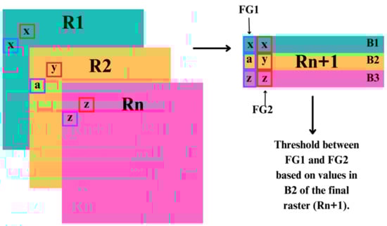
Figure 2.
Conceptual diagram of our classification approach of the freshwater and terrestrial–freshwater realm ecosystem functional groups into the Global Ecosystem Typology, stacking all created variable rasters (R1:Rn) into a singular raster (Rn+1) of multiple bands (B1:Bn), giving layers of information for each pixel (representative of ecosystem functional groups, W1 and W2), where numeric values (x,y,z,a) were used to identify thresholds among ecosystem functional groups.
To highlight and explore the temporally dynamic capabilities of the classification script, we explored variability of two large lakes, the freshwater Lake Numalla and saline Lake Wyara [57]. We compared the outputs of our algorithm in 2003–2008 and 2019–2024.
2.5. Validation of Results
To assess the validity of our classification maps, we compared them with independent spatially explicit observations. First, we compared our mapped results to two other wetland maps of the Paroo–Warrego area, the 1:250k Australian Wetlands layer (Kingsford et al. 2004 [11]) and the Australian National Aquatic Ecosystem (ANAE) Classification Framework (Australian Government Department of Climate Change, 2017 [22]) (Figure 1). We manually reclassified classifications in these two layers into the GET ecosystem functional groups, based on logical simple matching (Appendix I), comparing the percentages of each class across the three classification mapping approaches. We compared the percentage of classes to the total mapped freshwater and terrestrial–freshwater ecosystem realms in the area rather than directly comparing mapped area, as the mapping approaches differed. As our river mapping included a 30 m buffer, which, as a result included large areas of floodplain in the river GET functional groups, we compared the percentages of these classes including a 30 m buffer (necessary for inundation classification), but also to a 4 m buffer, which was more representative of actual river widths, meaning less floodplain area was classified as river area.
Next, we used ‘ground-truthed’ data in the form of wetlands surveyed from a low-flying aircraft (30–46 m above ground, 167 km/h) each year during the Australian Aerial Waterbird Surveys (1983–2024) [54]. For each wetland surveyed, we overlaid its GPS point onto our inundation maps. For consistency and to enhance reliability, we filtered the surveyed wetlands to include only those that had been surveyed more than once within the past 40 years. To accommodate GPS accuracy limitations due to low-altitude, high-speed flights (30–46 m above ground, 167 km/h), we applied a 200 m buffer around each survey point. Survey points are often estimated on approach to a wetland, further justifying the need for a buffer. Finally, we calculated the number of these buffered points that intersected with our mapped wetlands as a method of exploring the detection accuracy of the satellite inundation extent mapping.
We also created a validation dataset that included polygons surrounding 42 wetlands (not included in training datasets) based on wetlands with clear GET functional group allocations and that existed in the DEA Waterbodies mapped dataset [58]. This dataset included 14 different freshwater ecosystem functional groups, with three wetlands per IUCN GET ecosystem functional group (Appendix J). We manually pre-determined their best fitting IUCN GET ecosystem functional group based on inundation patterns [58], vegetation types present and visual inspections of shape (to determine whether natural or artificial). We then subsequently compared this manual classification to our classification script result. This validation approach explored the “real-world” accuracy of the classification system, which is reliant on multiple threshold models to work together to determine the correct classification, as described in Table 2.
Table 2.
Summarized decision rules and thresholds used to classify each of the ecosystem functional groups within the freshwater and transitional realms of the IUCN Global Ecosystem Typology within the Paroo–Warrego region, including classification challenges for each.
3. Results
We classified and mapped all 18 of the potential freshwater functional groups present across the Paroo–Warrego region using our automated classification approach (Figure 2, Table 2). Using thresholds and abiotic datasets, we produced high accuracy for most (83%) ecosystem functional groups, with three requiring additional mapping datasets. Sensitivity analyses examining the impact of a 20% variation in each threshold predictor variable on the final CART models revealed that accuracy remained consistently high despite these variations (Appendix K).
Importantly, the model distinguished ephemeral, seasonal and permanent waterbodies, based on their inundation signatures, achieving an overall accuracy of 83% (Figure 3). The best model was based on a mixture of mean and median inundation statistics during spring from September to November and summer from December to February (Figure 3, Appendix C). The sensitivity analysis revealed that a variation of up to 20% in any of the important predictor variables reduced the maximum accuracy to 73%, led by changes in mean inundation in September–November (Appendix K, Figure A7a). In practical terms, this means even a large variation in the most important predictor (mean inundation between September and November) would still result in a fairly accurate model.
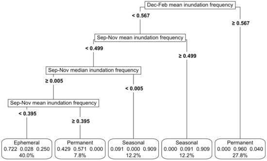
Figure 3.
CART models were used to develop inundation frequency thresholds among permanent, ephemeral and seasonal functional groups. The variables driving the splits at each node are displayed on the left, along with the numerical thresholds that separate the wetland types. These rules cumulatively defined the final thresholds, shown at the bottom for each wetland type: ephemeral, permanent and seasonal. The bubbles at the bottom indicated the proportion of each class within a node and the overall percentage of data attributed to that wetland type. For instance, in the far-right bubble, the threshold accounted for 27.8% of the total wetlands, with 96% classified as permanent, 4% as seasonal and none as ephemeral.
With only NDVI, we established thresholds with high accuracy (94%) among forested wetlands, marshes and non-vegetated wetlands (Figure 4, Appendix C). We also tried including EVI; however, it did not improve accuracies. In the model sensitivity analyses, a variation of up to 20% in the NDVI values resulted in a reduction of accuracy of 82%, led by the mean NDVI values as the most important predictor variable (Appendix K, Figure A7b).
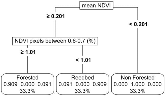
Figure 4.
Thresholding of the non-forested, forested and reedbed-based functional groups using NDVI. For details on interpretation, see the caption of Figure 2.
For natural and artificial wetlands, a CART model based on shape metrics alone achieved an accuracy of 73%, with square pixel and rectangular fitting metrics being the most important predictors (Figure 5). When NDVI thresholds were added, the accuracy increased to 87%, although the complexity of the thresholding also increased (Figure 6). Varying the predictor variables by up to 20% resulted in a decrease in accuracy to 69%, with the rectangular fitting shape metric identified as the most important predictor in driving accuracy changes (Appendix K, Figure A7c).

Figure 5.
Thresholding of the natural and artificial functional groups using shape metrics. For details on interpretation, see the caption of Figure 2.
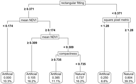
Figure 6.
Thresholding of the natural and artificial functional groups using both shape metrics and NDVI values. For details on interpretation, see the caption of Figure 2.
The random forest model distinguishing salt and freshwater wetlands achieved a final balanced accuracy score of 95% at the pixel level. The most important predictor variables were standard RGB and short-wave infrared bands (see Figure 7).

Figure 7.
Importance of satellite bands (features) in predicting salt or freshwater wetlands in the random forest modelling.
Shape metrics and NDVI values were useful in separating floodplains from terminal lakes (Figure 8), with an accuracy of 80%. A variation of up to 20% in the predictor variables resulted in a decrease in accuracy to 73%, with the compactness shape metric being the most important variable determining this accuracy variation (Appendix K, Figure A7d).
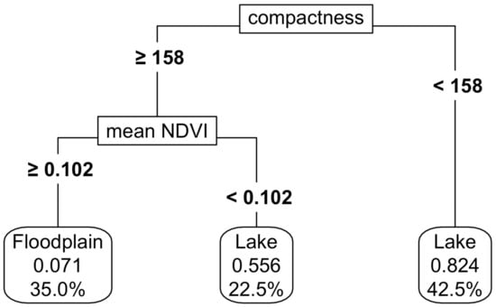
Figure 8.
Separation of the floodplains and terminal lakes using shape metrics and NDVI. For details on interpretation, see the caption of Figure 2.
The distributions of two ecosystem functional groups (F2.8 artesian springs and oasis and F3.1 large reservoirs) were obtained from external sources as they could not be mapped from remote sensing data and were not assessed for accuracy. The HydroLAKES dataset [46] was used to identify large permanent lakes, but this could have been done with satellite data, just at more computational cost.
Global Ecosystem Typology Classification
We successfully identified and mapped all relevant functional groups in the IUCN Global Ecosystem Typology using our derived thresholding values, which effectively separated out mutually exclusive functional groups, albeit with some challenges (Table 2).
Outputs included a stacked raster with 23 bands, the 22 data bands used to build the final classification and the classified raster band (Figure 9). Across the Paroo–Warrego area (13,689,186 ha, Figure 1), we identified over 128,880,408 distinct waterbodies covering an area of 1,024,904 ha (within the 99th percentile flooding surface water raster) (Figure 9). These were automatically thresholded into 10 relevant IUCN GET functional groups (Table 1), with functional groups greatly varying in proportion of wetland area (Table 3, Figure 9).

Figure 9.
Final classification map of Freshwater and Terrestrial–Freshwater transitional IUCN Global Ecosystem Typology ecosystem functional groups within the Paroo–Warrego area (2003–2023) in dryland Australia, highlighting (top left) the freshwater Lake Numalla (yellow) and saline Lake Wyara (purple), other areas of mixed episodic arid floodplain, fresh and saltwater lakes (bottom left) and constructed lacustrine wetlands and canals, misclassified as ephemeral salt lakes (bottom right).
Table 3.
The IUCN GET ecosystem functional groups as per the automated classification across the Paroo–Warrego region, with their area values and proportion of total classified wetland area as compared to the Australian Wetlands 250k and ANAE maps, as manually cross-referenced to the IUCN GET.
The most prominent ecosystem functional groups were F1.6 episodic arid rivers, TF 1.5 episodic arid floodplains and F2.5 ephemeral freshwater lakes, accounting for ~95% the area of freshwater and terrestrial–freshwater realms across the Paroo–Warrego region (Table 3). Comparing our classification to those of the Australian wetlands and ANAE, there was considerable similarity among those groups that could be compared (Table 3); however, not all GET functional groups were separated in current maps. Some differences in mapping approaches led to dissimilarities across some functional groups. For example, our approach of mapping Episodic arid rivers included a buffered area of floodplain, making it cover a significantly larger area than other mapping approaches. If arid rivers and floodplain were summed, the proportional extent of ecosystem functional groups on our map would be very similar to those in two other maps of the region (Table 3). The group with the largest discrepancy was the ephemeral freshwater lakes, which were likely being classified as floodplain in the two other mapping approaches.
Some canals were detected by satellite imagery but not present in the national dataset, and they were classified as either freshwater or saline ephemeral lakes in our approach (Figure 9). Temporal dynamism was an important part of our classification process. The temporally dynamic script showed that Lake Numalla is classified as part of the episodic arid floodplain in 2003–2008 and as a seasonal freshwater lake in 2019–2024 (Figure 10), but as an ephemeral freshwater lake overall (2000–2024, Figure 10).

Figure 10.
Temporal variation in classification in 2003–2008 (left) and 2019–2024 (right) of Lakes Numalla (seasonal freshwater lake, N) and Wyara (ephemeral salt lake, W) and other wetlands in the Paroo–Warrego region, resulting from classification and mapping using our thresholds for IUCN GET ecosystem functional groups.
In relation to validation, there were 138 wetlands surveyed more than once in the past 40 years by the Aerial Waterbird Survey (>1 ha) in the region, and 100 (72%) overlapped with our inundated wetlands. From the developed validation dataset of 42 wetlands, we found an 84% accuracy of perfect matches between the expected and classified IUCN GET ecosystem functional group. The most common misclassifications were for round, small, permanent and seasonal freshwater lakes, which were classified as constructed lacustrine wetlands due to their shape and flooding signatures.
4. Discussion
Classification of ecosystems is essential for managing and conserving biodiversity, especially in the face of escalating environmental challenges. Our objective, algorithmic mapping approach to classifying freshwater ecosystems in arid Australia was generally highly accurate, identifying the range of ecosystem functional groups under the Global Ecosystem Typology present in the area and, importantly, was a good match to current classifications. Importantly, the classification also identified a range of ecosystems functional groups not on existing maps of wetlands (e.g., artificial wetlands, artesian springs). Our approach not only required the development of thresholds to separate mutually exclusive ecosystem functional groups using satellite imagery, but it also required access to other mapping layers (e.g., dams and other artificial structures). The script-based framework allows for straightforward updates and improvements and enforces consistency across state borders, making it applicable to other regions in Australia and beyond.
The high accuracy of our thresholding approach (80–94%) across most ecosystem functional groups and the robustness of models in response to up to 20% variation in predictor variables showcased the utility of this tool. While examining natural variation in ecosystems is a valuable exercise, a 20% variation over datasets spanning 20 years would represent a substantial ecosystem shift. Ongoing acquisition of training data would continue to improve these models. This could be done by increasing wetland representation across arid Australia and other parts of the world, improving global applicability.
Such broadscale applications for functional ecosystem group thresholding models was already assisted by our collection of training data collection outside the Paroo–Warrego region. Our code not only correctly classified functional ecosystem groups but also effectively excluded those not in the Paroo–Warrego region. Whilst incorporating this extra variation at larger spatial scales may reduce accuracy within our study region, it allows for applicability to a wider area. This follows a model-based interpolation to unsampled sites approach [59], rather than prediction to new environments, which would be considered more similar to extrapolation or forecasting [59,60]. As scalability was important, we chose a potential loss of current accuracy for future wider applicability.
4.1. Current Limitations and Future Steps
The manual cross-referencing approach to classification, which requires pre-existing maps, can, according to the IUCN GET, allow for the transparent reporting of uncertainties by identifying plausible alternative functional groups and their respective likelihoods of correspondence or occurrence based on a percentile approach [14]. Simply, this means a singular wetland could be associated to two or more functional groups. Our current automated approach was binary—a functional group was classified as either one or another based on its dominant and most frequent characteristics. If required, our approach allows the modification and incorporation of uncertainties, using information from within the terminal nodes of the threshold models on the proportion of training records attributed to other functional groups as secondary attributes for each wetland.
This flexibility could be particularly relevant for ephemeral salt and freshwater lakes. Many of these transition throughout their flooding cycles, largely fresh when inundated, before becoming increasingly saline during drying [61]. This variability is defined in the categorization of F2.6 permanent salt and soda lakes, with spatial and temporal salinity gradients [14]. For simplicity and scalability, our salt model was dependent on the dominant or most frequent observation of the state of an ecosystem functional group for its classification as salt or freshwater within its 99% frequency extent.
Some ecosystem functional groups were more difficult to classify than others using remotely sensed data and are therefore dependent on static datasets. This is not ideal, given it does not capture the temporal variability of ecosystems. The static canal dataset was necessary because the 30 m resolution of Landsat satellite pixels was insufficient to detect narrow (<30 m wide) canals. Other canals may be subterranean, making surface water detection ineffective. Final classifications ultimately reflect data availability, exemplified by classification of some canals as ephemeral salt lakes because they were not in the static dataset (Figure 9). The resolution of Landsat data also limited the classification of small wetlands, including artificial farm dams. If <30 m, they would be indistinguishable. We added NDVI values to help distinguish natural from artificial ecosystems, but there was inevitably some misclassification of small natural round wetlands as artificial wetlands. This requires ground-truthing, but field validation was not a component of this study, with validation instead relying on other mapping products [22] and visual interpretation of satellite imagery. Sentinel data with 15 m resolution [62] could improve accuracy (also for the analysis of canals and river channels) but would result in larger processing times, which was not feasible in the currently utilized computing platform. Large reservoirs were also challenging in their separation from large natural lakes without high-resolution imagery or LiDAR data [63,64,65]. The man-made boundaries, such as dam walls, were hard to detect, and the large size of some reservoirs means they can take on natural shapes as they flood the landscape. Consequently, a static layer was also used for this ecosystem functional group. Locations of larger reservoirs are reasonably well known, and so the global reservoirs layer [46] was probably sufficiently accurate.
Floodplain functional groups were also challenging to classify. We classified them as all areas holding surface water, adjacent to a river channel, making them dependent on the accuracy of the river channels dataset. Problems can arise during large floods when extensive areas are inundated. Lakes can become connected to floodplains and rivers. This was the rationale for using the 99th percentile raster, excluding the 1 in 100 floods that connected an entire landscape, even though extreme floods are a natural part of the variation. Inevitably, some lakes become classified as floodplains, such as Lake Numalla (Figure 10). This is part of the challenge in the classification of highly dynamic systems.
We consolidated river channels within the mapping boundary by connecting all vectors into a singular river ecosystem functional group. This could be adjusted based on map boundaries or could be reevaluated every 100 km along a map, which might correspond to different river ecosystem functional groups based on elevation or temperature gradients.
Validation of the accuracy of the IUCN predicted ecosystem functional groups in the final outputs was problematic for a number of reasons. First, there are no universally accepted definitions or thresholds distinguishing between ephemerality, seasonality and permanency in terms of inundation patterns. Often, such classifications rely on expert knowledge rather than quantitative flooding data over more than a 40-year period. Our objective machine-based approach analyzed long-term trends and fluctuations capturing ecosystems natural variability. Contrastingly, ground visits provide for the inclusion of other biotic components or trophic networks to categorize freshwater ecosystems, not available from remote sensed data. For example, our analysis of remotely sensed data for Lake Numalla indicated a shift from freshwater lake to floodplain within the GET typology (Figure 10). But additional on-ground collected information such as invertebrate, macrophyte and waterbird abundance indicate consistent ecosystem features of a freshwater lake, regardless of the flooding regime [57]. Using flooding and other satellite data alone is necessary to cover large scales, allowing our modelling approach to separate IUCN GET ecosystem functional groups comprehensively, trained with data to separate ephemeral, seasonal and permanent flooding regimes objectively.
4.2. Extension of Approach
Currently, this automated approach has been developed specifically for freshwater ecosystem functional groups (Freshwater and Terrestrial–Freshwater realms [14]). Many freshwater ecosystem functional groups within the IUCN GET framework were successfully included or excluded from our classification, including additional functional groups finally not present in the study region. Our validation set of 40 wetlands were selected from a broader area outside the study region, and the high accuracies of this validation highlight that our approach is transferrable to other parts of Australia and the world, dependent upon further work to incorporate all functional groups present globally. For example, the mapping of “F2.9 Geothermal pools and wetlands” would require the identification of relevant satellite datasets, development of training data and recreation of thresholding models to separate this mutually exclusive functional group not currently mapped (as not present in Australia).
Several other adjustments would be necessary to globalize this approach, including the use of different surface water mapping datasets. We used the Water Observations from Space (WoFS) dataset, available across Australian and African continents in the Digital Earth Australia and Digital Earth Africa computing platforms [24,26]. Our freshwater mapping extent was therefore only as good as the WoFs dataset, which is limited when mapping flooded vegetation, and only applicable where this product is available. For a global application, other datasets such as those by Pekel, Cottam, Gorelick and Belward [13], and other developed surface water mapping indices [66], could be utilized. Other currently used static datasets would also need to be replaced with global products.
New seasonal analyses would be required to apply the approach to the northern hemisphere, varying from our September–November and December–February spring and summer timeframes. This would require relevant training data from the northern hemisphere and the development of new models to identify relevant seasonal thresholds.
For this project, which covered a large region of Australia, we used Australian software, providing access to different local datasets [23,24]. Currently the DEA Sandbox has strict size and memory limitations for standard users. Migrating to global platforms such as the Google Earth Engine might be the best approach to increasing the scalability and globalization of mapping [27,67].
Extending our approach to other realms is also possible with similar automated mapping. For example, the marine realm has many available global satellite and static datasets, probably useful in distinguishing marine ecosystem functional groups. For terrestrial ecosystem functional groups, soil and vegetation indices from satellites could be used. The subterranean realm could potentially use satellite GRACE data to track ground water storage and flow [68]. Generally, it is challenging to map subterranean systems around the world [69], and so it is often dependent on in situ mapping by robots or UAVs [70,71,72].
4.3. Benefits and Conservation and Management Value
Our automated approach offers several significant advantages over traditional manual classification systems and other typologies. Current manual approaches require the cross-referencing of each locality’s ecosystem functional groups, taking available maps, identifying common ecosystem features between the current map and the IUCN GET ecosystem functional groups and assigning old map units to the relevant IUCN GET ecosystem functional groups. This may be useful for connectivity with existing maps with legacy investments (e.g., databases, regulatory systems, large user networks) but a manual approach can be inconsistent and biased because it depends on expert opinion and pre-existing maps, with neither being always available. Where maps do exist, there are often ecosystem functional groups missing from the classification, particularly anthropogenic systems (e.g., F3 Artificial wetlands biome), including the constructed lacustrine wetlands and canals, ditches and drains, important inclusions in the Global Ecosystem Typology.
Leveraging widely available remote sensing data with advanced algorithms efficiently and objectively processes data over large areas of Earth’s surface where there is considerable variability. This, for most IUCN GET ecosystem functional groups, also does not depend on pre-existing classification maps. Automation ensures consistency, scalability, repeatability and temporal dynamism. Consistency across large scales is one of the most important features of this work ensuring classifications are comparable across spatial borders. For example, the main national vegetation map for Australia is actually a combination of state maps, all of which use different terminology, resolution and mapping techniques, therefore lacking consistency [73]. Further, while the latest updated version of this map was in 2020, the data represent on-ground dates of 1997 for extensive areas, with update years different for each state [73]. For freshwater ecosystems, the Australian National Aquatic Ecosystems map resolution differs across the continent, and with a focus mainly only on the Murray–Darling Basin, only parts of the map have been updated (last in 2021) [22,74]. In rapidly changing ecosystems, such as deforested rainforests, or highly variable systems like floodplains, a multi-year temporal lag before changes are recorded can significantly hinder conservation efforts. Delayed detection may reveal changes too late to take meaningful action, while seasonal variations may go entirely unrecorded. Additionally, changes in ecosystem extent are difficult to compare across countries. Even functionally similar ecosystems may be classified differently, underscoring the importance of a globally consistent classification system. Our method overcomes these challenges: first, by allowing for the selection of temporal periods to capture seasonal differences, and second, by utilizing satellite data and a scripted workflow for classification, updates can be performed every ~15 days.
These features make our approach particularly valuable for tracking progress towards conservation and management goals, including its application in the System of Environmental Economic Accounting. This system enables the contributions of the natural world to be quantified in monetary terms, allowing comparisons with other goods and services [75]. By doing so, it addresses critical themes such as biodiversity loss and climate change [75]. Effectiveness of this approach relies heavily on two factors: the availability of detailed ecosystem-level maps and the capacity to monitor changes over time, both factors addressed by our approach.
5. Conclusions
Our automated approach to classifying and mapping freshwater ecosystem functional groups, complying with IUCN GET, offers a scalable, dynamic and efficient alternative to manual cross-referencing methods. Our approach addresses many challenges inherent in ecosystem classification, including temporal variability and the complexities of large-scale environmental changes. Despite the current reliance on some static datasets for specific ecosystem functional groups, the successful implementation in the Paroo–Warrego region illustrated the effectiveness of our system, paving the way for future applications in other continents and ecosystems, dependent on extended training datasets. Our approach can contribute significantly to the conservation and management of biodiversity worldwide, including application within the System of Environmental Economic Accounting and the IUCN’s Red List of Ecosystems.
Author Contributions
Conceptualization, R.T.K., D.A.K., J.R.F.-P. and H.S.G.; methodology, R.J.F.; software, R.J.F.; validation, R.J.F.; formal analysis, R.J.F.; investigation, R.T.K., D.A.K., J.R.F.-P. and H.S.G.; resources, R.T.K., D.A.K., J.R.F.-P. and H.S.G.; data curation, R.J.F.; writing—original draft preparation, R.J.F.; writing—review and editing, R.T.K., D.A.K., J.R.F.-P. and H.S.G.; visualization, R.J.F.; supervision, R.T.K., D.A.K. and H.S.G.; project administration, R.T.K., D.A.K., J.R.F.-P. and H.S.G.; funding acquisition, R.T.K., D.A.K., J.R.F.-P. and H.S.G. All authors have read and agreed to the published version of the manuscript.
Funding
This research was funded by Bush Heritage Australia, the Centre for Ecosystem Science University of New South Wales, the Ian Potter Foundation and ARC Linkage Grant LP180100159.
Data Availability Statement
Example data and code will be made available upon request to corresponding author.
Conflicts of Interest
The authors declare no conflicts of interest.
Appendix A
Table A1.
Datasets used for classification mapping.
Table A1.
Datasets used for classification mapping.
| Purpose | Dataset | Citation |
|---|---|---|
| Surface Inundation | Water Observations from Space dataset (WOfS). | [35] |
| River channel mapping | National Surface Hydrology Database, Geoscience Australia. | [38] |
| Elevation | Geoscience Australia SRTM 1 s digital elevation model (ga_srtm_dem1sv1_0). | [24] |
| Minimum temperature | Monthly minimum gridded temperature NetCDFs from the Bureau of Meteorology, 2004–2022. | [39,40] |
| Minimum temperature | Monthly maximum gridded temperature NetCDFs from the Bureau of Meteorology, 2004–2022. | [39,40] |
| Precipitation | Monthly precipitation NetCDFs from the Bureau of Meteorology, 2004–2022. | [39,40] |
| Salt Vs Fresh | Geoscience Australia Landsat 8 Operational Land Imager and Thermal Infra-Red Scanner Analysis Ready Data Colletion 3 (ga_ls8c_ard_3). | [42,43] |
| Lake size and large reservoirs | HydroLAKES—Global database of all lakes with a size of at least 10 ha. | [46] |
| Springs | Compilation of: Springs of the Northern Territory, Springs of Queensland—Distribution and Assessment, Spring Locations Victoria, National Surface water points, a national tourist map ‘Australia Hot Springs Map’, and Global thermal spring distribution and relationship to endogenous and exogenous factors dataset. | [38,47,48,51,52,53] |
| Canals | National Surface Hydrology Database, Geoscience Australia. | [38] |
| NDVI and EVI | Geoscience Australia Sentinel 2A MSI Analysis Ready Data Collection 3 and Geoscience Australia Sentinel 2B MSI Analysis Ready Data Collection 3 (ga_s2am_ard_3 and ga_s2bm_ard_3). | [76,77,78] |
| Chlorophyll-a—NDCI | Geoscience Australia Sentinel 2A MSI Analysis Ready Data Collection 3 and Geoscience Australia Sentinel 2B MSI Analysis Ready Data Collection 3 (ga_s2am_ard_3 and ga_s2bm_ard_3). | [79,80] |
Appendix B
Table A2.
Table of ephemeral, seasonal and permanent wetlands used in the model training, with the relevant information used to assess their flooding patterns.
Table A2.
Table of ephemeral, seasonal and permanent wetlands used in the model training, with the relevant information used to assess their flooding patterns.
| Inundation Type | Wetland Name | Reference |
|---|---|---|
| Ephemeral | Bancannia Lake | [81] |
| Caryapundy Swamp | [82] | |
| Frome Swamp | [81] | |
| Goyders Lagoon | [83] | |
| Lake Acraman | [84] | |
| Lake Bathurst | [85] | |
| Lake Carnegie | [86] | |
| Lake Cowal | [87] | |
| Lake Cuddapan | [88] | |
| Lake Dey Dey | [84] | |
| Lake Frome | [89] | |
| Lake George | [90] | |
| Lake Hart | [84] | |
| Lake Hope | [84] | |
| Lake Mackay | [91] | |
| Lake Marroopootannie | [58] | |
| Lake Maurice | [84] | |
| Lake Murphy | [92] | |
| Lake Pinaroo | [93] | |
| Lake Torrens | [94] | |
| Lake Wombah | [95] | |
| Lake Woytchugga | [96] | |
| Lake Wyara | [97] | |
| Lake Yamma Yamma | [88] | |
| Naree Swamp 1 | Personal consultation with site managers of Naree Station, Bush Heritage | |
| Narran Lake (Back Lake) | [98] | |
| Nearie Lake | [98] | |
| Peery Lake | [99] | |
| Telephone Swamp | [100] | |
| Yantabulla Swamp | [101] | |
| Permanent | Bibra Lake | [102] |
| Darwin River Dam | [103] | |
| Herdsman Lake | [102] | |
| Kogolup N | [102] | |
| Kogolup S | [102] | |
| Lake Albert | [58] | |
| Lake Alexandrina | [104] | |
| Lake Argyle | [105] | |
| Lake Baghdad | [106] | |
| Lake Bullen Merri | [107] | |
| Lake Burley Griffin | [108] | |
| Lake corangamite | [109] | |
| Lake Dalrymple | [110] | |
| Lake Glenmaggie | [111] | |
| Lake Gnotuk | [112] | |
| Lake Goollelal | [102] | |
| Lake Gordon | [113] | |
| Lake Gwelup | [102] | |
| Lake Joondalup | [102] | |
| Lake Monger | [102] | |
| Lake Nowergup | [102] | |
| Lake Yonderup | [102] | |
| Loch McNess | [102] | |
| Manly Dam | [114] | |
| Mount Bold | [115] | |
| North Lake | [102] | |
| Ross River Dam | [116] | |
| Warragamba Dam | [117] | |
| Woronora Dam | [118] | |
| Yangebup Lake | [102] | |
| Seasonal | CB20 | [119] |
| CB38a | [119] | |
| CB4 | [119] | |
| CB5 | [119] | |
| CB82 | [119] | |
| Cungulla | [118] | |
| Downstream Lake Gore | [58] | |
| Horseshoe Bay Swamp | [116] | |
| Lake Carabooda | [102] | |
| Lake Coolongup | [102] | |
| Lake Gnangara | [102] | |
| Lake Jandabup | [102] | |
| Lake Muir | [58] | |
| Lake Neerabup | [102] | |
| Lake Sylvester | [120] | |
| Mount Brown Lake | [102] | |
| Serpentine Lagoon | [116] | |
| Toonpan Lagoon | [116] | |
| Unnamed | [58] | |
| Unnamed | [58] | |
| Unnamed | [58] | |
| Unnamed | [58] | |
| Unnamed | [58] | |
| Unnamed | [58] | |
| Unnamed | [58] | |
| Unnamed | [58] | |
| Unnamed | [58] | |
| Unnamed | [58] | |
| Unnamed | [58] | |
| Unnamed | [58] |
Appendix C
Table A3.
Calculated thresholds as visualized in Figure 3, Figure 4, Figure 5, Figure 6, Figure 7 and Figure 8.
| Type | Threshold |
|---|---|
| Permanent wetlands | Mean Dec–Feb inundation < 0.5670677, Mean Sep–Nov inundation < 0.4992318, and Mean Sep–Nov inundation ≥ 0.3947921 | Mean Dec–Feb inundation ≥ 0.5670677 |
| Seasonal wetlands | Mean Dec–Feb inundation < 0.5670677, Mean Sep–Nov inundation < 0.4992318, and Median Sep–Nov inundation < 0.004996511 | Mean Dec–Feb inundation < 0.5670677 and Mean Sep–Nov inundation ≥ 0.4992318 |
| Ephemeral wetlands | Mean Dec–Feb inundation < 0.5670677 and Median Sep–Nov inundation ≥ 0.004996511 and Mean Sep–Nov inundation < 0.3947921 |
| Artificial wetlands | Rectangular Fitting ≥ 0.371 & Mean NDVI < 0.174 | Rectangular Fitting ≥ 0.371 & Mean NDVI ≥ 0.31 | Rectangular Fitting < 0.371 & SquarePixelMetric < 1.28 | Rectangular Fitting ≥ 0.37 & Mean NDVI is 0.174 to 0.309 & Compactness ≥ 0.735 |
| Natural wetlands | Rectangular Fitting < 0.371 & SquarePixelMetric ≥ 1.28 | Rectangular Fitting ≥ 0.37 & Mean NDVI is 0.174 to 0.309 & Compactness < 0.735 |
| Non-forested wetlands | Mean NDVI < 0.201 |
| Forested wetlands | Mean NDVI ≥ 0.201 & proportion of pixels in the NDVI raster falling between 0.6 and 0.7 ≥ 1.01 |
| Marshes | Mean NDVI > 0.2 & proportion of pixels in the NDVI raster falling between 0.6 and 0.7 < 1.01 |
| Floodplains | Compactness ≥ 158 & Mean NDVI ≥ 0.102 |
Appendix D
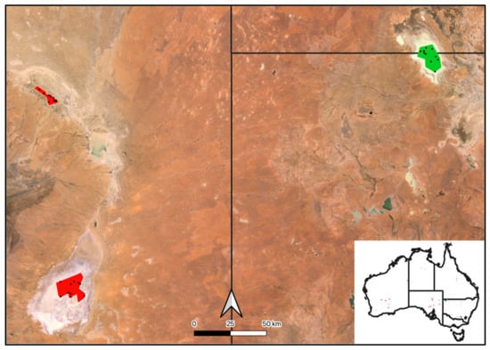
Figure A1.
Salt (red) and freshwater (green) polygons from which training points (dots) were extracted across Australia to train the random forest model to automate the classification of pixels into salt or freshwater categories.
Figure A1.
Salt (red) and freshwater (green) polygons from which training points (dots) were extracted across Australia to train the random forest model to automate the classification of pixels into salt or freshwater categories.
Appendix E

Figure A2.
Locations of hot springs according to the compiled springs datasets (Appendix C), including those identified within the Paroo Darling region (red).
Figure A2.
Locations of hot springs according to the compiled springs datasets (Appendix C), including those identified within the Paroo Darling region (red).
Appendix F
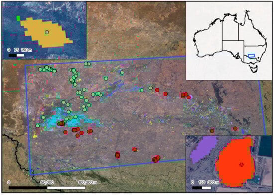
Figure A3.
Locations of the natural (green) and artificial (red) wetlands identified to train the shape metrics model.
Figure A3.
Locations of the natural (green) and artificial (red) wetlands identified to train the shape metrics model.
Appendix G
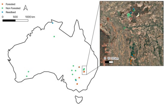
Figure A4.
Locations of forested, non-forested and reedbed based ecosystems across Australia.
Figure A4.
Locations of forested, non-forested and reedbed based ecosystems across Australia.
Appendix H
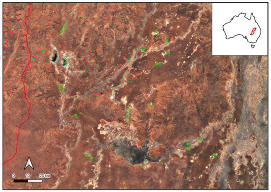
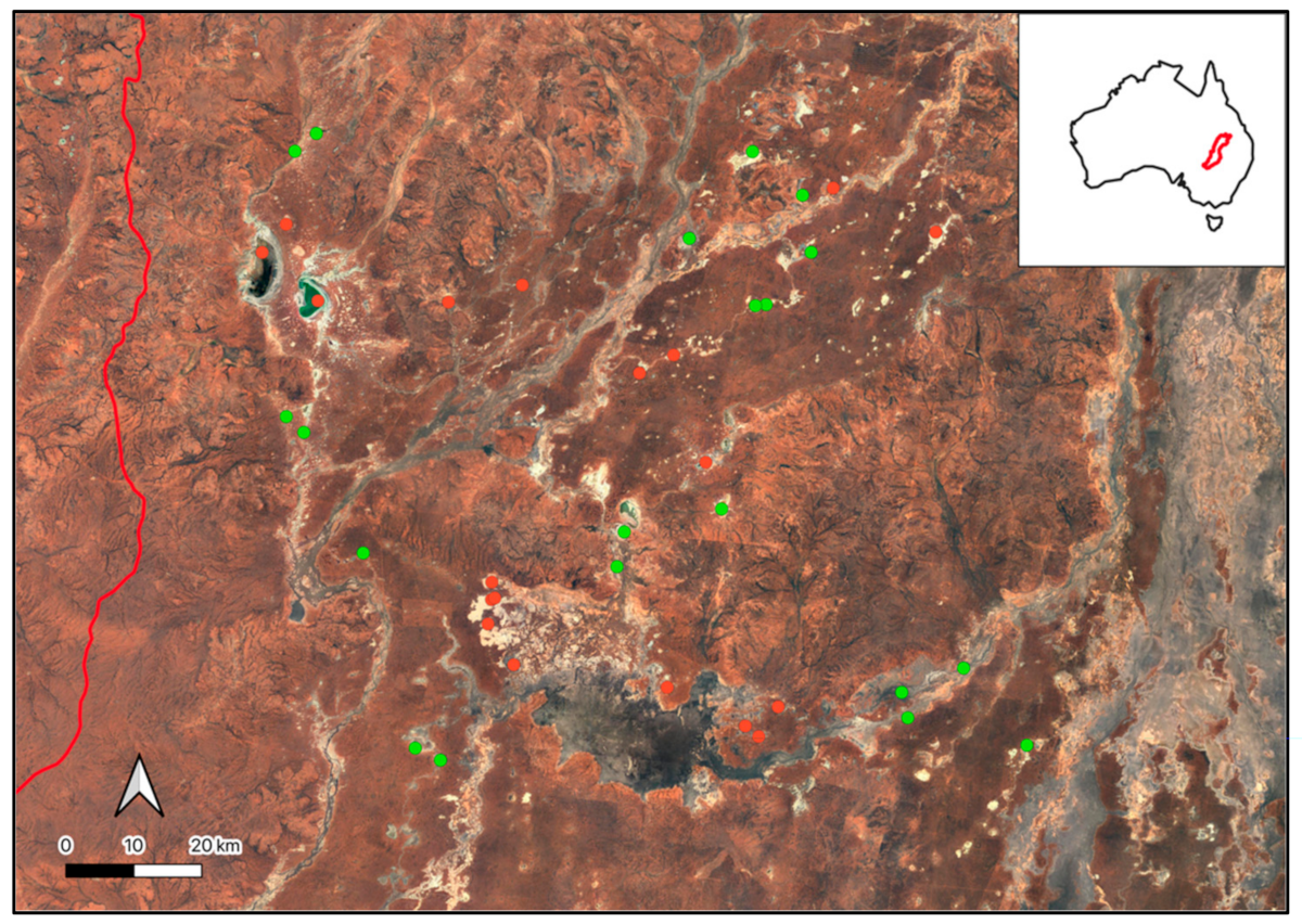
Figure A5.
Locations of floodplains (green) and lakes (red) used to separate the ecosystem functional groups with NDVI and shape metrics within the southern Paroo region of Australia (red border, inset).
Figure A5.
Locations of floodplains (green) and lakes (red) used to separate the ecosystem functional groups with NDVI and shape metrics within the southern Paroo region of Australia (red border, inset).
Appendix I
Table A4.
Manual cross-referencing of ANAE and 250k Wetland mapping classes to the GET.
Table A4.
Manual cross-referencing of ANAE and 250k Wetland mapping classes to the GET.
| GET Classification | ANAE Classification | Wetlands 250k Classification |
|---|---|---|
| Episodic arid river | Rt1.4: Temporary lowland stream + Rt1.2: Temporary transitional zone stream + Rt1: Temporary stream + Rt1.1: Temporary high energy upland stream + Rt1.3: Temporary low energy upland stream | Watercourse area |
| Small permanent freshwater lake | Lp1.1: Permanent lake + Pp4.2: Permanent wetland | Lake |
| Seasonal freshwater lakes | ||
| Ephemeral freshwater lakes | Lt1.1: Temporary lake + Pt3.1.2: Clay pan + Pt4.2: Temporary wetland | |
| Permanent salt and soda lakes | Lsp1.1: Permanent saline lake | |
| Ephemeral salt lakes | Lst1.1: Temporary saline lake + Pst2.2: Temporary salt marsh + Pst4: Temporary saline wetland + Pst1.1: Temporary saline swamp | |
| Artesian springs and oases | Pps5: Permanent spring | |
| Constructed lacustrine wetlands | Settling pond + Town rural storage | |
| Canals, ditches, and drains | ||
| Permanent marshes | Pp2.2.2: Permanent sedge/grass/forb marsh + Psp2.1: Permanent salt marsh + Pp2.1.2: Permanent tall emergent marsh | |
| Episodic arid floodplains | F2.2: Lignum shrubland riparian zone or floodplain + F1.10: Coolibah woodland and forest riparian zone or floodplain + F1.2: River red gum forest riparian zone or floodplain + Pt2.2.2: Temporary sedge/grass/forb marsh + F1.8: Black box woodland riparian zone or floodplain + F2.4: Shrubland riparian zone or floodplain + Pt1.8.2: Temporary shrub swamp + F1.4: River red gum woodland riparian zone or floodplain + Pt2.3.2: Freshwater meadow + Pt1.6.2: Temporary woodland swamp + F1.12: Woodland riparian zone or floodplain + F1.11: River cooba woodland riparian zone or floodplain + Pt1.2.2: Temporary black box swamp + Pt1.1.2: Temporary river red gum swamp + F1.13: Paperbark riparian zone or floodplain + Pt1.3.2: Temporary coolibah swamp + Pt2.1.2: Temporary tall emergent marsh + F4: Unspecified riparian zone or floodplain + Pt1.7.2: Temporary lignum swamp + F3.2: Sedge/forb/grassland riparian zone or floodplain | Land subject to inundation + Swamp |
Appendix J
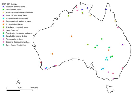
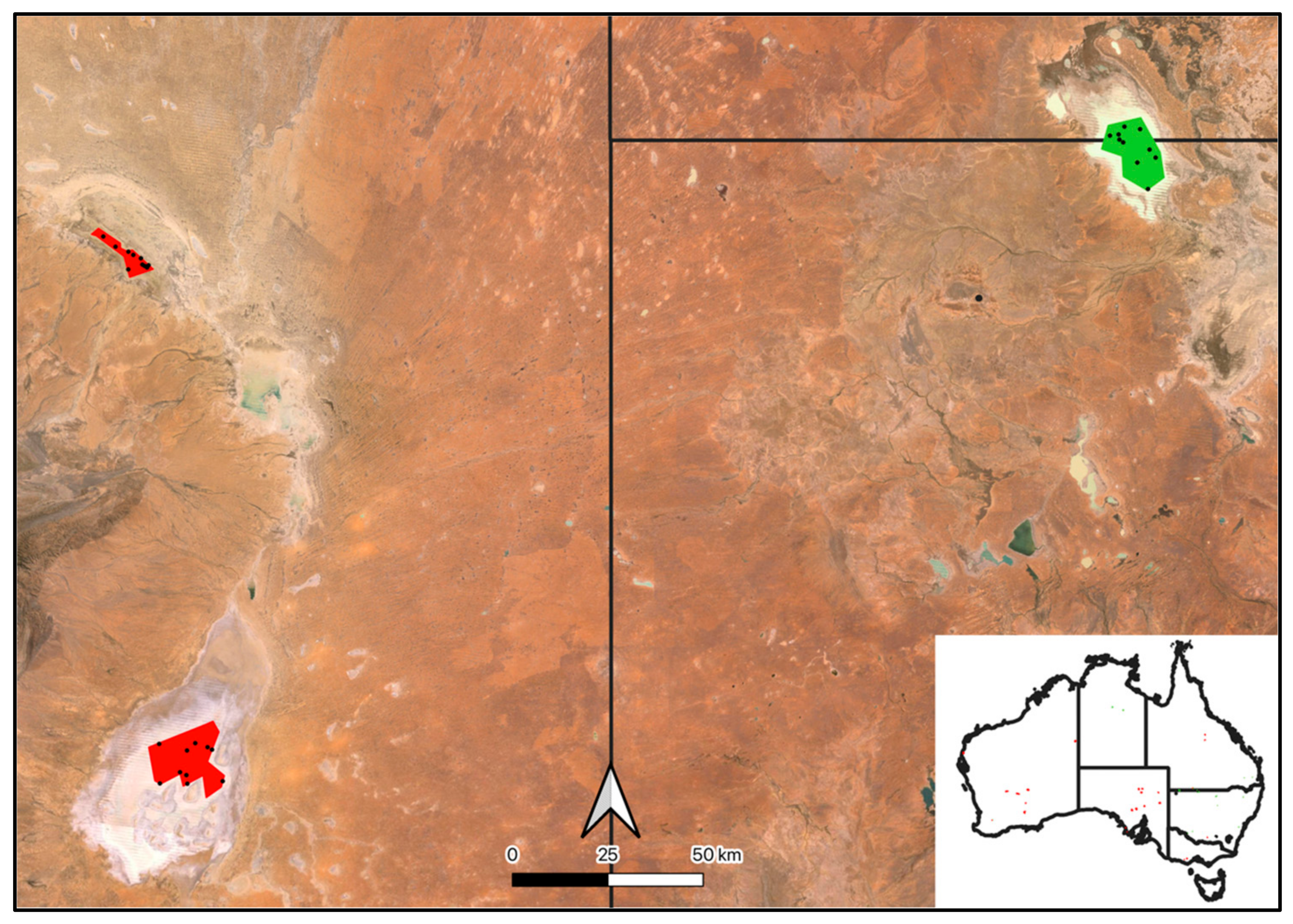
Figure A6.
Location and IUCN GET Classes of the wetlands used in the validation process of the automated scripting.
Figure A6.
Location and IUCN GET Classes of the wetlands used in the validation process of the automated scripting.
Appendix K
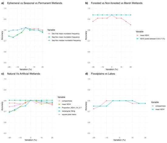
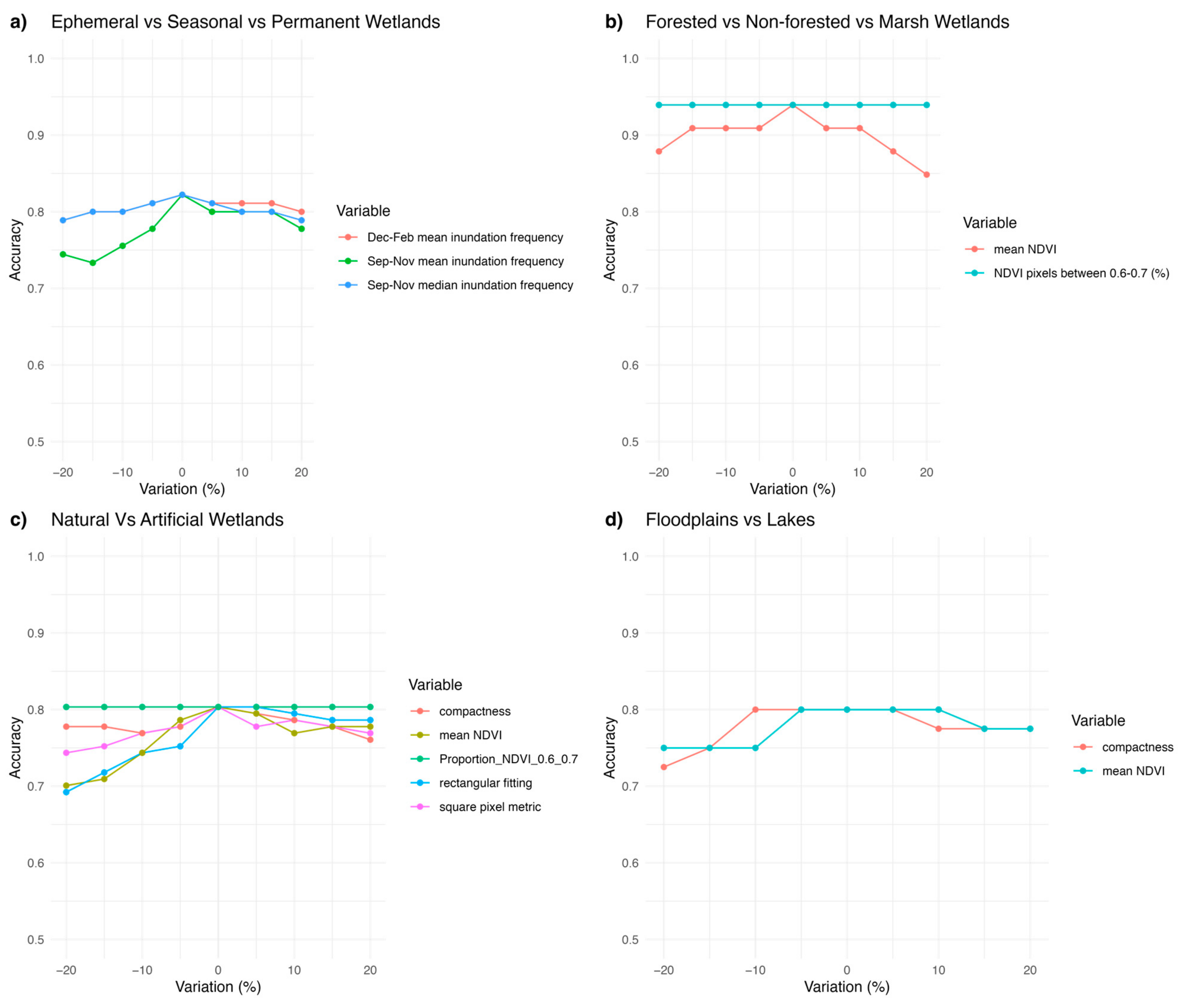
Figure A7.
Results of the sensitivity analyses conducted on the threshold modelling. Each plot title indicates the thresholding objective, while the listed variables represent the abiotic factors used in developing the thresholds. The x-axis shows the percentage change applied to each variable during the permutation analysis, and the y-axis illustrates the impact of these changes on overall thresholding accuracy.
References
- Nicholson, E.; Andrade, A.; Brooks, T.M.; Driver, A.; Ferrer-Paris, J.R.; Grantham, H.; Gudka, M.; Keith, D.A.; Kontula, T.; Lindgaard, A. Roles of the Red List of Ecosystems in the Kunming-Montreal Global Biodiversity Framework. Nat. Ecol. Evol. 2024, 8, 614–621. [Google Scholar] [CrossRef] [PubMed]
- Convention on Biological Diversity. Decision Adopted by the Conference of the Parties to the Convention on Biological Diversity 15/5; Monitoring framework for the Kunming-Montreal Global Biodiversity Framework (CBD/COP/DEC/15/5). 2022. Available online: https://www.cbd.int/doc/decisions/cop-15/cop-15-dec-05-en.pdf (accessed on 15 January 2025).
- Vörösmarty, C.J.; Rodríguez Osuna, V.; Cak, A.D.; Bhaduri, A.; Bunn, S.E.; Corsi, F.; Gastelumendi, J.; Green, P.; Harrison, I.; Lawford, R.; et al. Ecosystem-based water security and the Sustainable Development Goals (SDGs). Ecohydrol. Hydrobiol. 2018, 18, 317–333. [Google Scholar] [CrossRef]
- Green, P.A.; Vörösmarty, C.J.; Harrison, I.; Farrell, T.; Sáenz, L.; Fekete, B.M. Freshwater ecosystem services supporting humans: Pivoting from water crisis to water solutions. Glob. Environ. Chang. 2015, 34, 108–118. [Google Scholar] [CrossRef]
- Kingsford, R.T.; Basset, A.; Jackson, L. Wetlands: Conservation’s poor cousins. Aquat. Conserv. Mar. Freshwat. Ecosyst. 2016, 26, 892–916. [Google Scholar] [CrossRef]
- Kookana, R.S.; Drechsel, P.; Jamwal, P.; Vanderzalm, J. Urbanisation and emerging economies: Issues and potential solutions for water and food security. Sci. Total Environ. 2020, 732, 139057. [Google Scholar] [CrossRef]
- Mishra, B.K.; Kumar, P.; Saraswat, C.; Chakraborty, S.; Gautam, A. Water security in a changing environment: Concept, challenges and solutions. Water 2021, 13, 490. [Google Scholar] [CrossRef]
- Gxokwe, S.; Dube, T.; Mazvimavi, D. Multispectral remote sensing of wetlands in semi-arid and arid areas: A review on applications, challenges and possible future research directions. Remote Sens. 2020, 12, 4190. [Google Scholar] [CrossRef]
- Bowman, M. The Ramsar Convention on Wetlands: Has it made a difference? In Yearbook of International Cooperation on Environment and Development 2002–03; Stokke, O.S., Thommessen, O.B., Eds.; Routledge: London, UK, 2013; pp. 61–68. [Google Scholar]
- Hestir, E.L.; Brando, V.E.; Bresciani, M.; Giardino, C.; Matta, E.; Villa, P.; Dekker, A.G. Measuring freshwater aquatic ecosystems: The need for a hyperspectral global mapping satellite mission. Remote Sens. Environ. 2015, 167, 181–195. [Google Scholar] [CrossRef]
- Kingsford, R.; Brandis, K.; Thomas, R.; Crighton, P.; Knowles, E.; Gale, E. Classifying landform at broad spatial scales: The distribution and conservation of wetlands in New South Wales, Australia. Mar. Freshw. Res. 2004, 55, 17–31. [Google Scholar] [CrossRef]
- Timms, B.V. A comparison between saline and freshwater wetlands on Bloodwood Station, the Paroo, Australia, with special reference to their use by waterbirds. Int. J. Salt Lake Res. 1996, 5, 287–313. [Google Scholar] [CrossRef]
- Pekel, J.-F.; Cottam, A.; Gorelick, N.; Belward, A.S. High-resolution mapping of global surface water and its long-term changes. Nature 2016, 540, 418–422. [Google Scholar] [CrossRef] [PubMed]
- Keith, D.A.; Ferrer-Paris, J.R.; Nicholson, E.; Bishop, M.J.; Polidoro, B.A.; Ramirez-Llodra, E.; Tozer, M.G.; Nel, J.L.; Mac Nally, R.; Gregr, E.J. A function-based typology for Earth’s ecosystems. Nature 2022, 610, 513–518. [Google Scholar] [CrossRef] [PubMed]
- Jenkins, K.M.; Boulton, A.J.; Ryder, D.S. A common parched future? Research and management of Australian arid-zone floodplain wetlands. Hydrobiologia 2005, 552, 57–73. [Google Scholar] [CrossRef]
- Hu, S.; Niu, Z.; Chen, Y.; Li, L.; Zhang, H. Global wetlands: Potential distribution, wetland loss, and status. Sci. Total Environ. 2017, 586, 319–327. [Google Scholar] [CrossRef]
- Davidson, N.C. How much wetland has the world lost? Long-term and recent trends in global wetland area. Mar. Freshw. Res. 2014, 65, 934–941. [Google Scholar] [CrossRef]
- Zeitoun, M.; Goulden, M.; Tickner, D. Current and future challenges facing transboundary river basin management. Wiley Interdiscip. Rev. Clim. Chang. 2013, 4, 331–349. [Google Scholar] [CrossRef]
- Kingsford, R.T.; Boulton, A.J.; Puckridge, J.T. Challenges in managing dryland rivers crossing political boundaries: Lessons from Cooper Creek and the Paroo River, central Australia. Aquat. Conserv. Mar. Freshwat. Ecosyst. 1998, 8, 361–378. [Google Scholar] [CrossRef]
- Young, W.; Brandis, K.; Kingsford, R. Modelling monthly streamflows in two Australian dryland rivers: Matching model complexity to spatial scale and data availability. J. Hydrol. 2006, 331, 242–256. [Google Scholar] [CrossRef]
- Bureau of Meteorology. Monthly Rainfall Wanaaring Post Office. 2024. Available online: http://www.bom.gov.au/climate/data/ (accessed on 9 April 2025).
- Australian Government Department of Climate Change, Energy, the Environment and Water. Australian National Aquatic Ecosystem (ANAE) Classification for the Murray Darling Basin—Wetlands (2017). Available online: https://researchdata.edu.au/australian-national-aquatic-wetlands-2017/2985595 (accessed on 3 February 2025).
- Krause, C.; Dunn, B.; Bishop-Taylor, R.; Adams, C.; Burton, C.; Alger, M.; Chua, S.; Phillips, C.; Newey, V.; Kouzoubov, K.; et al. Digital Earth Australia Notebooks and Tools Repository; Geoscience Australia: Canberra, Australia, 2021. [Google Scholar] [CrossRef]
- Dhu, T.; Dunn, B.; Lewis, B.; Lymburner, L.; Mueller, N.; Telfer, E.; Lewis, A.; McIntyre, A.; Minchin, S.; Phillips, C. Digital Earth Australia–unlocking new value from earth observation data. Big Earth Data 2017, 1, 64–74. [Google Scholar] [CrossRef]
- Kumar, M. Distributed Execution of Dask on HPC: A Case Study. In Proceedings of the 2023 World Conference on Communication & Computing (WCONF), Raipur, India, 14–16 July 2023; pp. 1–4. [Google Scholar]
- Digital Earth Africa. Digital Earth Africa. Available online: https://www.digitalearthafrica.org (accessed on 25 June 2024).
- Gorelick, N.; Hancher, M.; Dixon, M.; Ilyushchenko, S.; Thau, D.; Moore, R. Google Earth Engine: Planetary-scale geospatial analysis for everyone. Remote Sens. Environ. 2017, 202, 18–27. [Google Scholar] [CrossRef]
- Meyer, H.; Pebesma, E. Predicting into unknown space? Estimating the area of applicability of spatial prediction models. Methods Ecol. Evol. 2021, 12, 1620–1633. [Google Scholar] [CrossRef]
- Leigh, C.; Sheldon, F.; Kingsford, R.T.; Arthington, A.H. Sequential floods drive ‘booms’ and wetland persistence in dryland rivers: A synthesis. Mar. Freshw. Res. 2010, 61, 896–908. [Google Scholar] [CrossRef]
- Carter, V. An overview of the hydrologic concerns related to wetlands in the United States. Can. J. Bot. 1986, 64, 364–374. [Google Scholar] [CrossRef]
- Frazier, P.; Page, K.; Louis, J.; Briggs, S.; Robertson, A. Relating wetland inundation to river flow using Landsat TM data. Int. J. Remote Sens. 2003, 24, 3755–3770. [Google Scholar] [CrossRef]
- Stromberg, J.C.; Hazelton, A.F.; White, M.S.; White, J.M.; Fischer, R.A. Ephemeral wetlands along a spatially intermittent river: Temporal patterns of vegetation development. Wetlands 2009, 29, 330–342. [Google Scholar] [CrossRef]
- Brönmark, C.; Hansson, L.-A. The Biology of Lakes and Ponds, 3rd ed.; Oxford University Press: Oxford, UK, 2017. [Google Scholar]
- Sheldon, F.; Boulton, A.J.; Puckridge, J.T. Conservation value of variable connectivity: Aquatic invertebrate assemblages of channel and floodplain habitats of a central Australian arid-zone river, Cooper Creek. Biol. Conserv. 2002, 103, 13–31. [Google Scholar] [CrossRef]
- Mueller, N.; Lewis, A.; Roberts, D.; Ring, S.; Melrose, R.; Sixsmith, J.; Lymburner, L.; McIntyre, A.; Tan, P.; Curnow, S. Water observations from space: Mapping surface water from 25 years of Landsat imagery across Australia. Remote Sens. Environ. 2016, 174, 341–352. [Google Scholar] [CrossRef]
- Therneau, T.; Atkinson, B.; Ripley, B. rpart: Recursive Partitioning and Regression Trees. 2023. Available online: https://cran.r-project.org/web/packages/rpart/rpart.pdf (accessed on 9 April 2025).
- Massada, A.B.; Carmel, Y. Incorporating output variance in local sensitivity analysis for stochastic models. Ecol. Model. 2008, 213, 463–467. [Google Scholar] [CrossRef]
- Crossman, S.; Li, O. Surface Hydrology Lines (National). 2015. Available online: https://pid.geoscience.gov.au/dataset/ga/83130 (accessed on 3 February 2025).
- Jones, D.A.; Wang, W.; Fawcett, R. High-quality spatial climate data-sets for Australia. Aust. Meteorol. Oceanogr. J. 2009, 58, 233. [Google Scholar] [CrossRef]
- Evans, A.; Jones, D.; Smalley, R.; Lellyett, S. An Enhanced Gridded Rainfall Analysis Scheme for Australia; National Library of Australia Cataloguing: Canberra, ACT, Australia, 2020; pp. 55–67. [Google Scholar]
- Wang, J.; Bastrakova, I.; Evans, B.; Kemp, C.; Fraser, R.; Wyborn, L. Bringing Australian Geophysical Data onto a High Performance Data Node at the National Computational Infrastructure; Society of Exploration Geophysicists: Houston, TX, USA, 2015. [Google Scholar]
- Safaee, S.; Wang, J. Towards global mapping of salt pans and salt playas using Landsat imagery: A case study of western United States. Int. J. Remote Sens. 2020, 41, 8693–8716. [Google Scholar] [CrossRef]
- Ding, M.; Wang, J.; Song, C.; Sheng, Y.; Hutchinson, J.S.; Langston, A.L.; Marston, L. A framework of freshwater and saline lake typology classification through leveraging hydroclimate, spectral, and literature evidence. J. Hydrol. 2024, 632, 130704. [Google Scholar] [CrossRef]
- Gislason, P.O.; Benediktsson, J.A.; Sveinsson, J.R. Random forests for land cover classification. Pattern Recog. Lett. 2006, 27, 294–300. [Google Scholar] [CrossRef]
- Rodriguez-Galiano, V.F.; Ghimire, B.; Rogan, J.; Chica-Olmo, M.; Rigol-Sanchez, J.P. An assessment of the effectiveness of a random forest classifier for land-cover classification. ISPRS J. Photogramm. Remote Sens. 2012, 67, 93–104. [Google Scholar] [CrossRef]
- Messager, M.L.; Lehner, B.; Grill, G.; Nedeva, I.; Schmitt, O. Estimating the volume and age of water stored in global lakes using a geo-statistical approach. Nat. Commun. 2016, 7, 13603. [Google Scholar] [CrossRef]
- Department of Environment Parks and Water Security. Springs of the Northern Territory. 2013. Available online: https://www.ntlis.nt.gov.au/metadata/export_data?metadata_id=E9D78F668FC02B33E040CD9B214403C3&type=html (accessed on 3 February 2025).
- Queensland Herbarium, E.P.A. Springs of Queensland—Distribution and Assessment Bioregional Assessment Source Dataset. 2006. Available online: https://data.gov.au/data/dataset/82749253-f555-47d9-ba76-7140c55b2a65 (accessed on 20 February 2025).
- Department of Environment Land Water & Planning Victoria. Spring Locations. 2023. Available online: https://discover.data.vic.gov.au/dataset/spring-locations (accessed on 9 April 2025).
- Crossman, S.; Li, O. Surface Hydrology Points (Regional). 2015. Available online: https://pid.geoscience.gov.au/dataset/ga/83132 (accessed on 3 February 2025).
- Tamburello, G.; Chiodini, G.; Ciotoli, G.; Procesi, M.; Rouwet, D.; Sandri, L.; Carbonara, N.; Masciantonio, C. Global thermal spring distribution and relationship to endogenous and exogenous factors. Nat. Commun. 2022, 13, 6378. [Google Scholar] [CrossRef]
- Top Hot Springs. Hot Springs in Australia. 2023. Available online: https://www.google.com/maps/d/viewer?mid=1NqcZITjfiGuOrNeILYuYGBgfWsPMzu6v&hl=en_US&ll=-27.118820089943387%2C134.50052323328015&z=5 (accessed on 20 February 2025).
- Erfurt, P. The Conservation of Hot Springs. In The Geoheritage of Hot Springs; Springer: Cham, Switzerland, 2021; pp. 91–118. [Google Scholar]
- Kingsford, R.T.; Porter, J.L.; Brandis, K.J.; Ryall, S. Aerial surveys of waterbirds in Australia. Sci. Data 2020, 7, 172. [Google Scholar] [CrossRef]
- Westinga, E.; Beltran, A.P.R.; De Bie, C.A.; van Gils, H.A. A novel approach to optimize hierarchical vegetation mapping from hyper-temporal NDVI imagery, demonstrated at national level for Namibia. Int. J. Appl. Earth Obs. Geoinf. 2020, 91, 102152. [Google Scholar] [CrossRef]
- Thomas, R.F.; Kingsford, R.T.; Lu, Y.; Cox, S.J.; Sims, N.C.; Hunter, S.J. Mapping inundation in the heterogeneous floodplain wetlands of the Macquarie Marshes, using Landsat Thematic Mapper. J. Hydrol. 2015, 524, 194–213. [Google Scholar] [CrossRef]
- Kingsford, R.; Porter, J. Waterbirds on an adjacent freshwater lake and salt lake in arid Australia. Biol. Conserv. 1994, 69, 219–228. [Google Scholar] [CrossRef]
- Krause, C.E.; Newey, V.; Alger, M.J.; Lymburner, L. Mapping and monitoring the multi-decadal dynamics of Australia’s open waterbodies using Landsat. Remote Sens. 2021, 13, 1437. [Google Scholar] [CrossRef]
- Elith, J.; Leathwick, J.R. Species distribution models: Ecological explanation and prediction across space and time. Annu. Rev. Ecol. Evol. Syst. 2009, 40, 677–697. [Google Scholar] [CrossRef]
- Araujo, M.B.; Pearson, R.G.; Thuiller, W.; Erhard, M. Validation of species–climate impact models under climate change. Glob. Chang. Biol. 2005, 11, 1504–1513. [Google Scholar] [CrossRef]
- Costelloe, J.F.; Grayson, R.B.; McMahon, T.A.; Argent, R.M. Spatial and temporal variability of water salinity in an ephemeral, arid-zone river, central Australia. Hydrol. Process. Int. J. 2005, 19, 3147–3166. [Google Scholar] [CrossRef]
- Phiri, D.; Simwanda, M.; Salekin, S.; Nyirenda, V.R.; Murayama, Y.; Ranagalage, M. Sentinel-2 data for land cover/use mapping: A review. Remote Sens. 2020, 12, 2291. [Google Scholar] [CrossRef]
- Yousefi, N.; Ralph, T.J.; Farebrother, W.; Chang, H.-C.; Hesse, P.P. Assessment of channel expansion and contraction using cross-section data from repeated LiDAR acquisitions in the Macquarie Marshes, NSW. In Proceedings of the 9th Australian Stream Management Conference, Hobart, Australia, 2–15 August 2018; pp. 12–15. [Google Scholar]
- Krishna Paladugu, B.S.; Torrent, D.G. Automated water runoff location in large canal networks. In Proceedings of the Construction Research Congress 2018, New Orleans, MA, USA, 2–4 April 2018; pp. 760–769. [Google Scholar]
- Schmidt, J.; Rabiger-Völlmer, J.; Werther, L.; Werban, U.; Dietrich, P.; Berg, S.; Ettel, P.; Linzen, S.; Stele, A.; Schneider, B. 3D-Modelling of Charlemagne’s Summit Canal (Southern Germany)—Merging Remote Sensing and Geoarchaeological Subsurface Data. Remote Sens. 2019, 11, 1111. [Google Scholar] [CrossRef]
- Zhou, Y.; Dong, J.; Xiao, X.; Xiao, T.; Yang, Z.; Zhao, G.; Zou, Z.; Qin, Y. Open surface water mapping algorithms: A comparison of water-related spectral indices and sensors. Water 2017, 9, 256. [Google Scholar] [CrossRef]
- Zhou, B.; Okin, G.S.; Zhang, J. Leveraging Google Earth Engine (GEE) and machine learning algorithms to incorporate in situ measurement from different times for rangelands monitoring. Remote Sens. Environ. 2020, 236, 111521. [Google Scholar] [CrossRef]
- Joodaki, G.; Wahr, J.; Swenson, S. Estimating the human contribution to groundwater depletion in the Middle East, from GRACE data, land surface models, and well observations. Water Resour. Res. 2014, 50, 2679–2692. [Google Scholar] [CrossRef]
- Mammola, S.; Altermatt, F.; Alther, R.; Amorim, I.R.; Băncilă, R.I.; Borges, P.A.; Brad, T.; Brankovits, D.; Cardoso, P.; Cerasoli, F. Perspectives and pitfalls in preserving subterranean biodiversity through protected areas. npj Biodivers. 2024, 3, 2. [Google Scholar] [CrossRef]
- Rouček, T.; Pecka, M.; Čížek, P.; Petříček, T.; Bayer, J.; Šalanský, V.; Heřt, D.; Petrlík, M.; Báča, T.; Spurný, V. Darpa subterranean challenge: Multi-robotic exploration of underground environments. In Proceedings of the Modelling and Simulation for Autonomous Systems: 6th International Conference, MESAS 2019, Palermo, Italy, 29–31 October 2019; Revised Selected Papers 6. 2020; pp. 274–290. [Google Scholar]
- Silver, D.; Ferguson, D.; Morris, A.; Thayer, S. Topological exploration of subterranean environments. J. Field Robot. 2006, 23, 395–415. [Google Scholar] [CrossRef]
- Martz, J.; Al-Sabban, W.; Smith, R.N. Survey of unmanned subterranean exploration, navigation, and localisation. IET Cyber-Syst. Robot. 2020, 2, 1–13. [Google Scholar] [CrossRef]
- Australian Government Department of Climate Change, Energy, the Environment and Water. National Vegetation Information System (NVIS) Version 6.0—Extant Vegetation. 2020. Available online: https://gis.environment.gov.au/gispubmap/rest/services/ogc_services/NVIS_ext_mvg/MapServer (accessed on 20 February 2025).
- Brooks, S. ANAE Classification of the Murray-Darling Basin Technical Report, Revision 3.0; Technical Report for the Commonwealth Environmental Water Office; Department of Agriculture, Water and the Environment: Canberra, Australia, 2021. [Google Scholar]
- United Nations. System of Environmental Economic Accounting. Available online: https://seea.un.org/ecosystem-accounting (accessed on 16 January 2025).
- Rouse, J.W., Jr.; Haas, R.H.; Schell, J.; Deering, D. Monitoring the Vernal Advancement and Retrogradation (Green Wave Effect) of Natural Vegetation. 1973. Available online: https://ntrs.nasa.gov/citations/19750020419 (accessed on 20 February 2025).
- Huete, A.; Didan, K.; Miura, T.; Rodriguez, E.P.; Gao, X.; Ferreira, L.G. Overview of the radiometric and biophysical performance of the MODIS vegetation indices. Remote Sens. Environ. 2002, 83, 195–213. [Google Scholar] [CrossRef]
- Digital Earth Australia. Vegetation Phenology. Available online: https://knowledge.dea.ga.gov.au/notebooks/Real_world_examples/Vegetation_phenology/#Getting-started (accessed on 3 November 2024).
- Digital Earth Australia. Monitoring Chlorophyll-a in Australian Waterbodies. Available online: https://knowledge.dea.ga.gov.au/notebooks/Real_world_examples/Chlorophyll_monitoring (accessed on 13 November 2024).
- Mishra, S.; Mishra, D.R. Normalized difference chlorophyll index: A novel model for remote estimation of chlorophyll-a concentration in turbid productive waters. Remote Sens. Environ. 2012, 117, 394–406. [Google Scholar] [CrossRef]
- NSW Government. North-Western NSW. Available online: https://water.dpie.nsw.gov.au/about-us/learn-about-water/basins-and-catchments/catchments/north-western-nsw (accessed on 10 November 2024).
- NSW National Parks and Wildlife Service. Narriearra Caryapundy Swamp National Park. Available online: https://www.nationalparks.nsw.gov.au/visit-a-park/parks/narriearra-caryapundy-swamp-national-park/what-we-are-doing (accessed on 10 November 2024).
- Birdlife International. Important Bird Area Factsheet: Goyder Lagoon (Australia). Available online: https://datazone.birdlife.org/site/factsheet/goyder-lagoon-iba-australia (accessed on 2 December 2024).
- Sheldon, F. Spencer Regions Strategic Water Management Study: Environmental Flow Criteria; Department for Environment Heritage and Aboriginal Affairs. 1999. Available online: https://ewater.org.au/archive/crcfe/freshwater/publications.nsf/8116917c22b76d58ca256f120027bb83/02d7ff6c71e3302fca256f0f0014b32a/%24FILE/SheldonSPENCER.pdf (accessed on 20 February 2025).
- Department of Climate Change Energy the Environment and Water. Directory of Important Wetlands in Australia. 2021. Available online: https://www.dcceew.gov.au/water/wetlands/australian-wetlands-database/directory-important-wetlands (accessed on 9 April 2025).
- NASA. Filling up Lake Carnegie. Available online: https://earthobservatory.nasa.gov/images/146628/filling-up-lake-carnegie (accessed on 10 November 2024).
- Liu, X.; Watts, R.J.; Allan, C. Local ecological knowledge and wise use of ephemeral wetlands: The case of the Cowal system, Australia. Wetl. Ecol. Manag. 2023, 31, 791–804. [Google Scholar] [CrossRef]
- Geological and Bioregional Assessment Program. DIWA Lake Condition: Endpoint Node Description for the Cooper GBA Region. Available online: https://gba-explorer.bioregionalassessments.gov.au/coo/items/item/64/0 (accessed on 10 November 2024).
- National Parks and Wildlife Service South Australia. Vulkathunha-Gammon Ranges National Park. Available online: https://www.parks.sa.gov.au/parks/vulkathunha-gammon-ranges-national-park (accessed on 10 November 2024).
- Australian Geographic. The Amazing Disappearing Lake. Available online: https://www.australiangeographic.com.au/travel/travel-destinations/2011/09/the-amazing-disappearing-lake-george (accessed on 10 November 2024).
- NASA. Australia’s Ephemeral Lake Mackay. Available online: https://earthobservatory.nasa.gov/images/84984/australias-ephemeral-lake-mackay (accessed on 10 November 2024).
- Halford, J.; Fensham, R. Vegetation and environmental relations of ephemeral subtropical wetlands in central Queensland, Australia. Aust. J. Bot. 2014, 62, 499–510. [Google Scholar] [CrossRef]
- NSW Government Environment and Heritage. Lake Pinaroo (Fort Grey Basin). Available online: https://www2.environment.nsw.gov.au/topics/water/wetlands/internationally-significant-wetlands/lake-pinaroo-fort-grey-basin (accessed on 10 November 2024).
- NASA. Lake Torrens Is a Lake Again. Available online: https://earthobservatory.nasa.gov/images/150566/lake-torrens-is-a-lake-again (accessed on 10 November 2024).
- NSW National Parks and Wildlife Service. Brindingabba National Park; 2024. Available online: https://www.environment.nsw.gov.au/-/media/OEH/Corporate-Site/Documents/Parks-reserves-and-protected-areas/Parks-statement-of-management-intent/brindingabba-national-park-statement-of-management-intent-20240071.pdf (accessed on 9 April 2025).
- Eastwood, K. Lake Reborn. Available online: https://www.outbackmag.com.au/lake-reborn (accessed on 10 November 2024).
- Queensland Wetlands Program. Currawinya Lakes—A Wetland of International Importance. 2014. [Google Scholar]
- NSW National Parks and Wildlife Service. Narran Lake Nature Reserve Plan of Management; 2000. Available online: https://www.environment.nsw.gov.au/-/media/OEH/Corporate-Site/Documents/Parks-reserves-and-protected-areas/Parks-plans-of-management/narran-lake-nature-reserve-plan-of-management-000095.pdf (accessed on 9 April 2025).
- Volkofsky, A. Peery Lake and Paroo River Wetlands Fill in Once-in-a-Decade Outback Event. Available online: https://www.abc.net.au/news/2020-07-01/peery-lake-and-paroo-river-wetlands-fill/12387172 (accessed on 2 December 2024).
- State of New South Wales and Department of Environment and Climate Change. In Ecological Character Description: Lake Pinaroo Ramsar Site; 2008. Available online: https://www.environment.nsw.gov.au/-/media/OEH/Corporate-Site/Documents/Water/Wetlands/ecological-character-description-lake-pinaroo-ramsar-site-080275.pdf (accessed on 2 February 2025).
- Carroll, G. The Biggest Rains in 30 Years. Available online: https://www.bushheritage.org.au/news/the-biggest-rains-in-30-years (accessed on 10 November 2024).
- Crowns, J.; Davis, J.; Cheal, F.; Schmidt, L.; Rosich, R.; Bradley, S. Multivariate pattern analysis of wetland invertebrate communities and environmental variables in Western Australia. Aust. J. Ecol. 1992, 17, 275–288. [Google Scholar] [CrossRef]
- PowerWater. Darwin River Dam Level. Available online: https://www.powerwater.com.au/about/what-we-do/water-supply/darwin-water-supply/darwin-river-dam (accessed on 2 December 2024).
- Department of Agriculture Water and the Environment. Coorong and Lakes Alexandrina and Albert Ramsar Wetland—Fact sheet. Available online: https://www.dcceew.gov.au/water/wetlands/publications/coorong-and-lakes-alexandrina-and-albert-ramsar-wetland-factsheet (accessed on 2 December 2024).
- Australia’s North West. Lake Argyle. Available online: https://www.australiasnorthwest.com/explore/kimberley/lake-argyle (accessed on 2 December 2024).
- Rottnest Island Authority. Watch the Salt Pans Come Alive. Available online: https://www.rottnestisland.com/see-do/wildlife-nature/lakes-salt-lakes#:~:text=Many%20of%20Rottnest%20Island’s%20salt,wetland%20fixtures%20of%20the%20island (accessed on 10 November 2024).
- Agriculture Victoria. Lake Bullen Merri. Available online: https://vro.agriculture.vic.gov.au/dpi/vro/coranregn.nsf/pages/corangamite_eruption_points_bullen_merri (accessed on 2 December 2024).
- Authority, N.C. Lake Burley Griffin. Available online: https://www.nca.gov.au/attractions/lake-burley-griffin# (accessed on 2 December 2024).
- Colac Otway Shire Council. Lake Corangamite Nature Reserve. Available online: https://www.colacotway.vic.gov.au/Parks-Recreation/Lake-Corangamite-Nature-Reserve (accessed on 2 December 2024).
- Queensland Government. Burdekin Dam (Lake Dalrymple). Available online: https://www.daf.qld.gov.au/rsa/sips-dams-and-weirs/profile?dam=burdekin-dam (accessed on 2 December 2024).
- Southern Rural Water. Lake Glenmaggie. Available online: https://www.srw.com.au/recreation/locations/lake-glenmaggie (accessed on 2 December 2024).
- Agriculture Victoria. Lake Gnotuk. Available online: https://vro.agriculture.vic.gov.au/dpi/vro/coranregn.nsf/pages/corangamite_eruption_points_gnotuk (accessed on 2 December 2024).
- Discover Tasmania. Lake Gordon—Lake Pedder—Strathgordon. Available online: https://www.discovertasmania.com.au/things-to-do/nature-and-wildlife/lakegordonlakepedderstrathgordon (accessed on 2 December 2024).
- Northern Beaches Council. Manly Dam. Available online: https://www.northernbeaches.nsw.gov.au/things-to-do/parks-and-trails/parks/manly-dam (accessed on 2 December 2024).
- SA Water. Mount Bold Reservoir. Available online: https://www.sawater.com.au/water-and-the-environment/south-australias-water-sources/reservoir-data/mount-bold-reservoir (accessed on 2 December 2024).
- Lukacs, G. Wetlands of the Townsville Area; Australian Centre for Tropical Freshwater Research, James Cook University: Douglas, Australia, 1996; Available online: http://www.soe-townsville.org/data/actfr_reports/tcc_wetlands_actfr96.pdf (accessed on 2 February 2025).
- WaterNSW. Warragamba Dam. Available online: https://www.waternsw.com.au/nsw-dams/greater-sydney-dams/warragamba-dam (accessed on 2 December 2024).
- WaterNSW. Woronora Dam. Available online: https://www.waternsw.com.au/nsw-dams/greater-sydney-dams/woronora-dam (accessed on 2 December 2024).
- Halse, S.; Shiel, R.; Storey, A.; Edward, D.; Lansbury, I.; Cale, D.; Harvey, M. Aquatic invertebrates and waterbirds of wetlands and rivers of the southern Carnarvon Basin, Western Australia. Rec. West. Aust. Mus. Suppl. 2000, 61, 217–265. [Google Scholar] [CrossRef]
- Harrison, L.; McGuire, L.; Ward, S.; Fisher, A.; Pavey, C.; Fegan, M.; Lynch, B.; Australia, N.H.T.; Lake Sylvester System; Northern Territory. Department of Natural Resources, Environment, The Arts and Sport. Biodiversity Conservation Unit. Division of Environment, Heritage and the Arts. 2009. Available online: https://digitalntl.nt.gov.au/10070/532053/0/2 (accessed on 2 February 2025).


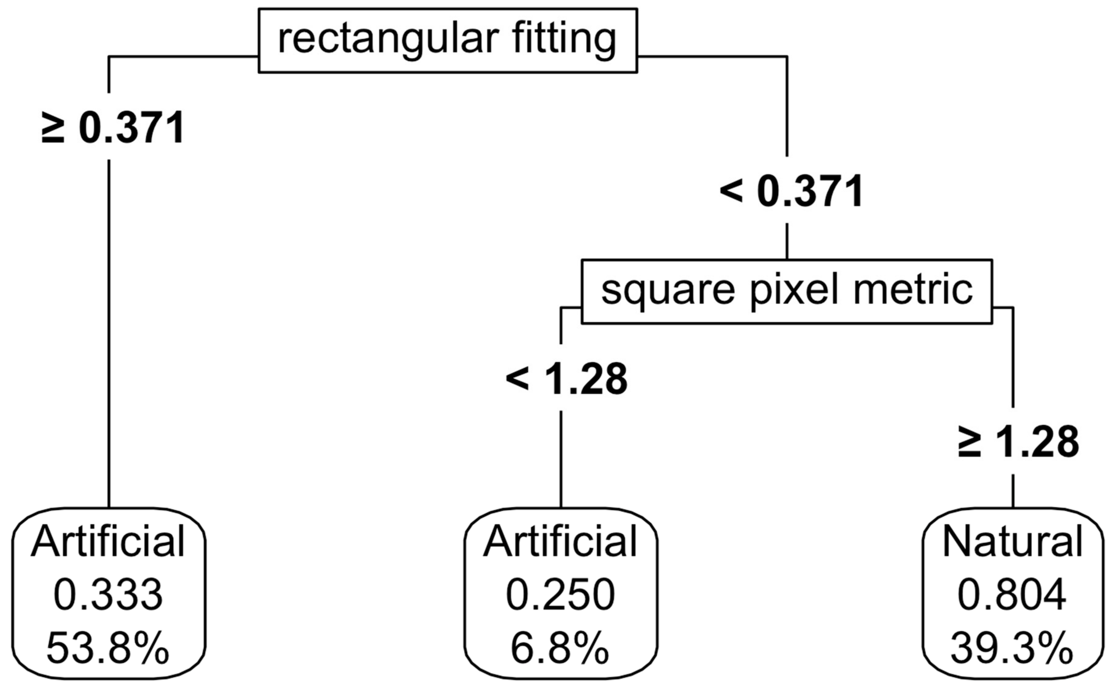

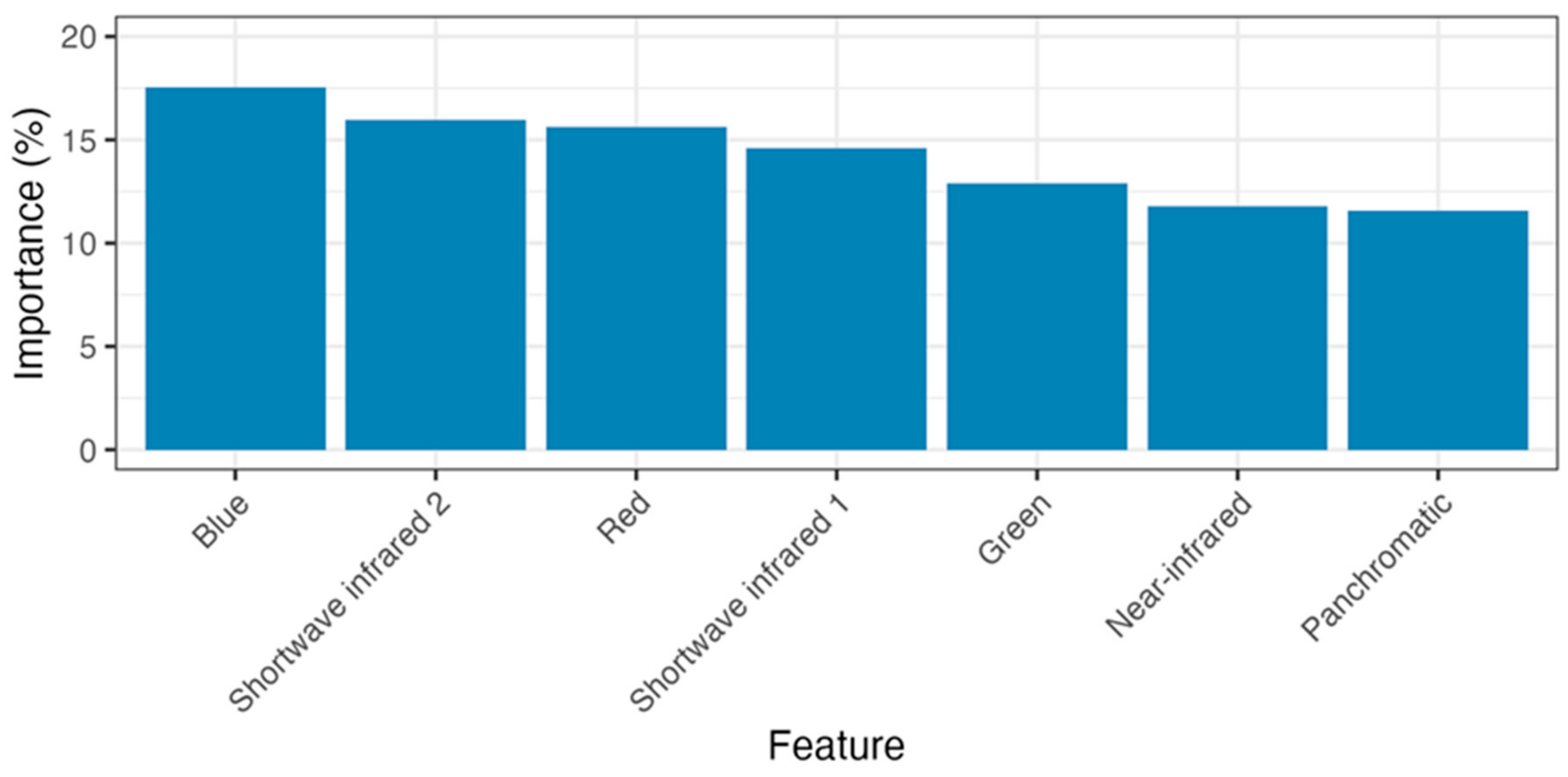

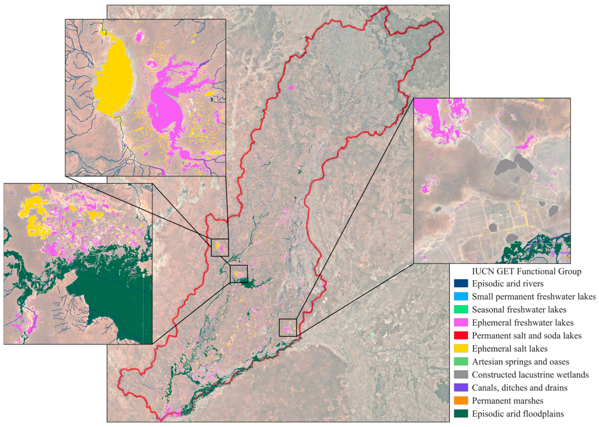
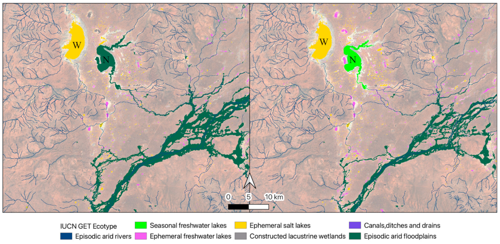
Disclaimer/Publisher’s Note: The statements, opinions and data contained in all publications are solely those of the individual author(s) and contributor(s) and not of MDPI and/or the editor(s). MDPI and/or the editor(s) disclaim responsibility for any injury to people or property resulting from any ideas, methods, instructions or products referred to in the content. |
© 2025 by the authors. Licensee MDPI, Basel, Switzerland. This article is an open access article distributed under the terms and conditions of the Creative Commons Attribution (CC BY) license (https://creativecommons.org/licenses/by/4.0/).