SWOT-Based Intertidal Digital Elevation Model Extraction and Spatiotemporal Variation Assessment

Abstract

Traditional methods for the construction of intertidal digital elevation models (DEMs) require the integration of long-term multi-sensor datasets and struggle to capture the spatiotemporal variation caused by ocean dynamics. The SWOT (surface water and ocean topography) mission, with its wide-swath interferometric altimetry technology, provides instantaneous full-swath elevation data in a single pass, offering a revolutionary data source for high-precision intertidal topographic monitoring. This study presents a framework for SWOT-based intertidal DEM extraction that integrates data preprocessing, topographic slope map construction, and tidal channel masking. The radial sand ridge region along the Jiangsu coast is analyzed using SWOT L2 LR (Low Resolution) unsmoothed data from July 2023 to December 2024. Multisource validation data are used to comprehensively assess the accuracy of sea surface height (SSH) and land elevation derived from LR products. Results show that the root mean square error (RMSE) of SSH at Dafeng, Yanghe, and Gensha tide stations is 0.25 m, 0.19 m, and 0.32 m, respectively. Validation with LiDAR data indicates a land elevation accuracy of ~0.3 m. Additionally, the topographic features captured by LR products are consistent with the patterns observed in the remote sensing imagery. A 16-month time-series analysis reveals significant spatiotemporal variations in the Tiaozini area, particularly concentrated in the tidal channel areas. Furthermore, the Pearson correlation coefficient for the DEMs generated from SWOT data decreased from 0.94 over a one-month interval to 0.84 over sixteen months, reflecting the persistent impact of oceanic dynamic processes on intertidal topography.

1. Introduction

The intertidal zone, as a transition area between land and sea, is characterized by unique ecological, morphological, and hydrological features, playing a crucial role in maintaining ecosystem stability and protecting biodiversity [1,2,3]. In the context of global climate change, the rise of the sea level presents new threats to the intertidal zone, potentially exacerbating coastal erosion, altering sediment distribution, and leading to ecosystem degradation [4,5,6,7]. This highlights the urgency of dynamic monitoring and scientific management of the intertidal zone [8]. Digital elevation models (DEMs) are key tools for mapping the topographic features of the intertidal zone and play an indispensable role in tidal flat research [9,10,11]. It is capable of accurately delineating the terrain undulations and topographic details of the intertidal zone, aiding in the in-depth study of tidal flat evolution [12]. Furthermore, high-precision DEMs provide critical data support and scientific evidence in coastal disaster monitoring, resource management, ecological protection, and climate change mitigation.

However, high-precision DEM modeling in the intertidal zone still faces numerous challenges. Traditional methods for intertidal DEM construction include airborne light detection and ranging (LiDAR) [13,14], waterline-based methods [15,16,17], satellite-derived bathymetry (SDB) [18,19], multibeam sounding [20], and synthetic aperture radar interferometry (InSAR) [21,22,23]. Airborne LiDAR generates high-precision topographic models by emitting laser pulses and recording their return times, which directly calculate three-dimensional point cloud coordinates [24]. This method achieves centimeter-level resolution and accuracy in exposed tidal flats but is associated with high data acquisition costs and is constrained by penetration capabilities and airspace regulations. The waterline-based method extracts instantaneous waterlines at various tidal levels using multi-temporal satellite imagery. It infers elevation values for each waterline based on tidal data and constructs continuous topographic surfaces via spatial interpolation [25]. It is suitable for gently sloping tidal flats but is sensitive to steep terrains, rapid tidal fluctuations, and cloud cover, thus requiring long-term data accumulation. SDB combines laser altimetry data from the ice, cloud, and land elevation satellite-2 (ICESat-2) with multispectral imagery (e.g., Sentinel-2), along with regression analysis algorithms, to model intertidal topography. It provides high spatial resolution and extensive coverage for DEM modeling, but may result in increased measurement errors under complex aquatic conditions [26,27]. Multibeam sounding collects underwater topographic data through shipborne sonar and is ideal for high-precision mapping in deep-water regions; however, it is limited by the accessibility of equipment in the intertidal zone and cannot measure terrestrial topography [28,29]. InSAR uses phase difference information from radar satellites imaging the same region from different orbital positions, combined with geometric baseline parameters, to calculate surface elevation. While this method achieves centimeter-level accuracy in terrestrial areas and provides wide-swath altimetry capabilities, changes in surface moisture induced by tidal inundation can cause signal decorrelation in traditional InSAR technology [21,30].

It is evident that there are two major challenges when modeling intertidal DEM using traditional methods. On one hand, it requires the synergistic integration of multiple sensor datasets to obtain sufficient and accurate data (e.g., SDB and waterline-based method), which reduces modeling efficiency. On the other hand, the area experiences significant spatiotemporal changes in topography due to tidal effects. However, due to limitations in sensor penetration capabilities and revisit frequency, long-term data accumulation is needed to complete DEM modeling, making it difficult to accurately capture the time-varying signals.

The surface water and ocean topography (SWOT) mission, developed jointly by the National Aeronautics and Space Administration (NASA) and the French National Center for Space Studies (Centre national d’études spatiales, CNES), was successfully launched on 16 December 2022 [31,32]. It became the first satellite mission equipped with wide-swath interferometric altimetry capability for water surface elevation measurements. The satellite carries the Ka-band radar interferometer (KaRIn), which uses a dual antenna configuration to form an interferometric baseline, enabling high-precision measurement of water surface elevation while simultaneously capturing water body extent (120 km across track). This provides a revolutionary data source for high-precision monitoring of intertidal zones. Compared to traditional methods, SWOT can obtain wide-swath elevation information in a single pass, eliminating the issue of temporal mismatch in multi-pass data used in traditional methods [31]. Moreover, it can operate independently of tide gauge data, making it indispensable for remote areas without tide gauges. With a 21-day revisit cycle, SWOT facilitates efficient and accurate automated production and dynamic updates of large-scale intertidal DEMs, driving the transition from static modeling to the analysis of time-varying signals in coastal topography monitoring.

Currently, SWOT has been applied innovatively in various oceanographic fields, such as ocean tides, internal waves, mesoscale ocean currents, and coastal zone monitoring, demonstrating its broad application potential [33,34,35]. Salameh et al. (2024) have preliminarily validated the feasibility of using SWOT data to extract intertidal DEMs [36], while Hart-Davis et al. (2024) assessed its altimetry performance in coastal tidal monitoring [33]. Liu et al. (2024) and Xue et al. (2024) analyzed SWOT’s performance in extracting DEM information in inland areas, highlighting its potential in monitoring lake and land surface changes [37,38]. However, there remains a lack of a reliable framework for extracting intertidal DEMs from SWOT data, and further research is needed on its capability to detect time-varying signals and capture spatial detail. Additionally, the applicability and performance of the SWOT data in intertidal DEM extraction require thorough analysis. This study proposes a DEM extraction algorithm based on slope maps and evaluates the capabilities of SWOT LR (Low Resolution) products in DEM extraction. Furthermore, the spatiotemporal variations of intertidal zone topography are analyzed. The specific organization of this research is as follows: Section 2 introduces the research area, SWOT data, and validation data; Section 3 details the DEM derivation method based on SWOT data; Section 4 provides an in-depth performance analysis of SWOT-derived DEM; Section 5 discusses the ability of SWOT data in capturing detailed surface features; and finally, Section 6 presents the conclusions.

2. Data and Study Area

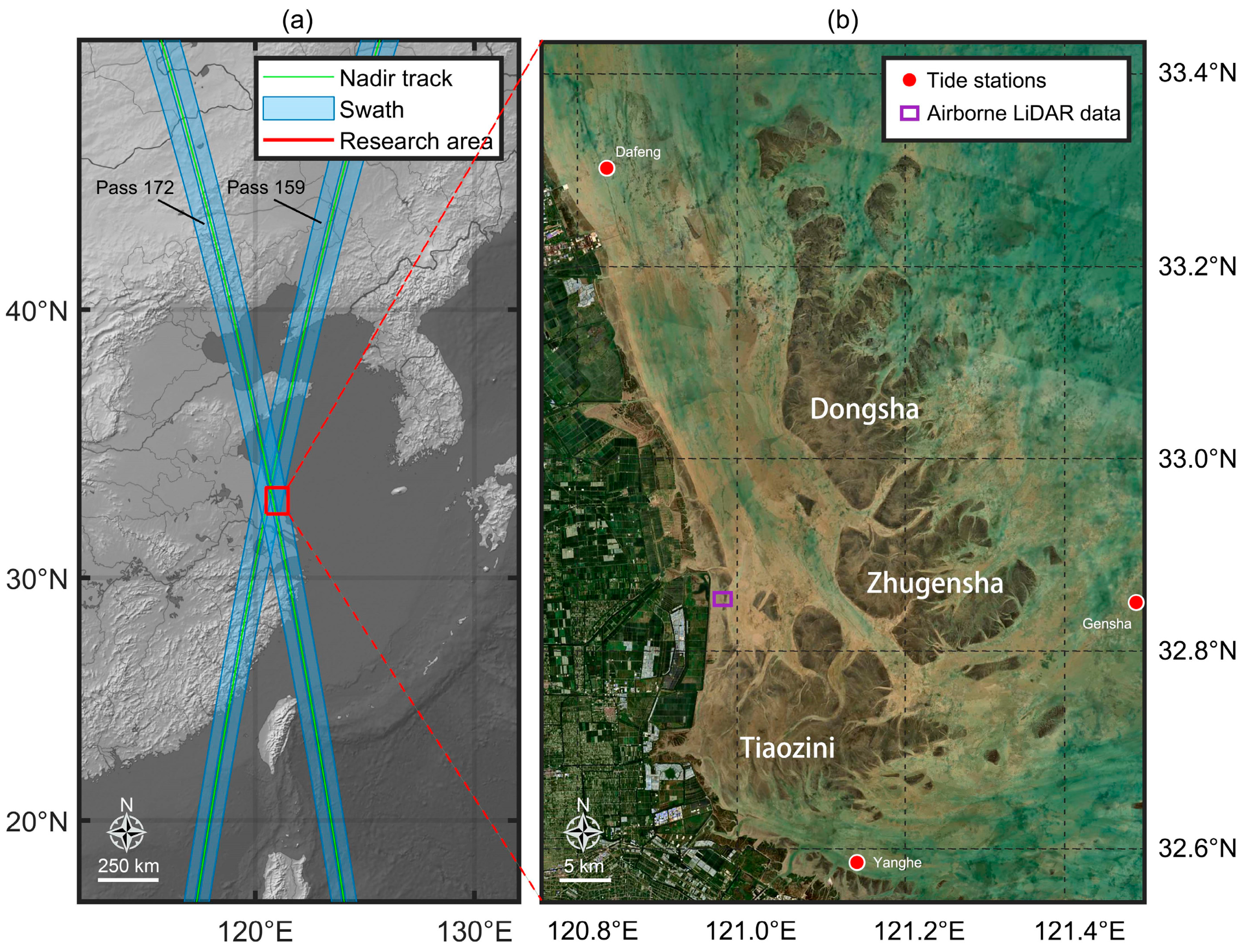
2.1. Study Area

The research area is focused on the tidal flats of the radial tidal sand ridges in the coastal area off Central Jiangsu, north of the Yangtze River Delta (red box in Figure 1a). Spanning over 100 km from north to south, this region is formed by sediments from the Yellow, Huai, and Yangtze Rivers converging at the boundary between the Yellow Sea and the East China Sea [15,39,40]. As shown in Figure 1b, the sand ridges encompass three key regions: Tiaozini (32.6°N–32.85°N, 120.95°E–121.25°E), ZhugenSha (32.78°N–32.95°N, 121.13°E–121.40°E), and Dongsha (32.95°N–33.15°N, 121.05°E–121.35°E), which are characterized by silty mudflats and feature low-lying terrain. As one of the characteristic intertidal zones along the coast of Eastern China, it holds significant ecological and economic value and plays a critical role in mitigating natural disasters like storm surges.

Strong tidal influences result in significant spatiotemporal changes in tidal flat morphology [41]. The tidal regime is primarily semi-diurnal, with tidal ranges typically ranging from 2–4 m but capable of exceeding 9 m in the Tiaozini area [42]. These pronounced tidal variations lead to complex and diverse tidal flat topographies, influenced by daily and seasonal tidal fluctuations. The dynamic interplay between tidal cycles and hydrodynamic forces continually alters the tidal flats. Therefore, detailed investigations into the intertidal topography of this region provide essential data support and theoretical foundations for environmental protection, disaster prevention, and ecological restoration. Additionally, the complex environment enables the performance validation of SWOT-derived intertidal DEM.

2.2. SWOT Data

Since July 2023, NASA and CNES have begun releasing SWOT L2 products for the science orbit, including the LR products and the HR (High resolution) products for ocean and inland water applications, respectively (https://www.earthdata.nasa.gov/). This study employs 50 tracks of SWOT data from July 2023 to December 2024 (with 25 tracks each from PASS 159 and PASS 172) for intertidal DEM extraction. The distribution of the tracks and swath coverage is illustrated in Figure 1a by green solid lines and blue polygons, respectively. Considering the data gaps of the HR data within the study area, the SWOT L2 LR unsmooth product with a spatial resolution of 250 m is employed for DEM extraction and performance evaluation. Additionally, the SWOT L3 LR product, which is derived from the L2 LR product after further error corrections by CNES, is utilized in this study. Both the L2 and L3 products use the WGS-84 reference ellipsoid. (https://www.aviso.altimetry.fr/en/missions/current-missions/swot/public-release-of-the-swot-level-3-l3-product.html, accessed on 21 April 2025). Building on the corrections provided by the L2 LR product, the L3 LR product incorporates multi-altimetry mission corrections (including crossover adjustments, cross-track phase error, and tilt correction), noise reduction using convolutional neural network technology, and outlier removal [43]. These enhancements significantly improve the signal-to-noise ratio and reduce systematic errors in SWOT data. However, due to potential misidentification issues in intertidal zones caused by outlier removal, this study only uses the calibration information from the L3 product.

2.3. Tide Gauge Data

The tide information from three stations, including Dafeng Station (32.28°N, 120.82°E), Yanghe Station (32.57°N, 121.14°E), and Gensha Station (32.84°N, 121.49°E), are derived from the China National Marine Data and Information Service (https://global-tide.nmdis.org.cn/), with a temporal resolution of 10 min and referenced to the WGS-84 (World Geodetic System 1984) system. The locations of the tide gauge stations are illustrated by red scatters in Figure 1b. Specifically, Dafeng Station and Yanghe Station are located ~1 km from the coast, while Gensha Station is located 50 km offshore in open waters. This arrangement facilitates the validation of sea surface altimetry accuracy under varying conditions. It is important to note that the data period for Dafeng Station is from July 2023 to December 2024, while it is from April 2023 to December 2024 for both Yanghe Station and Gensha Station.

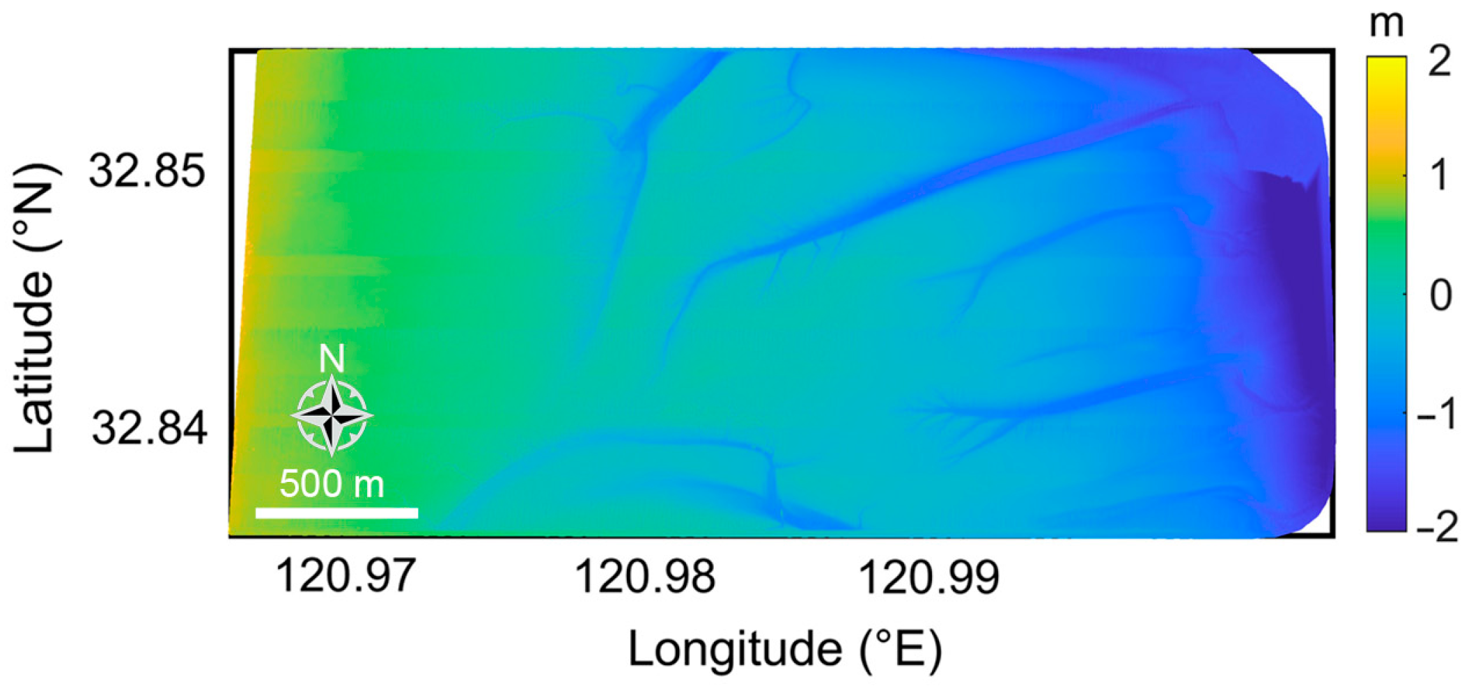
2.4. Airborne Lidar Data

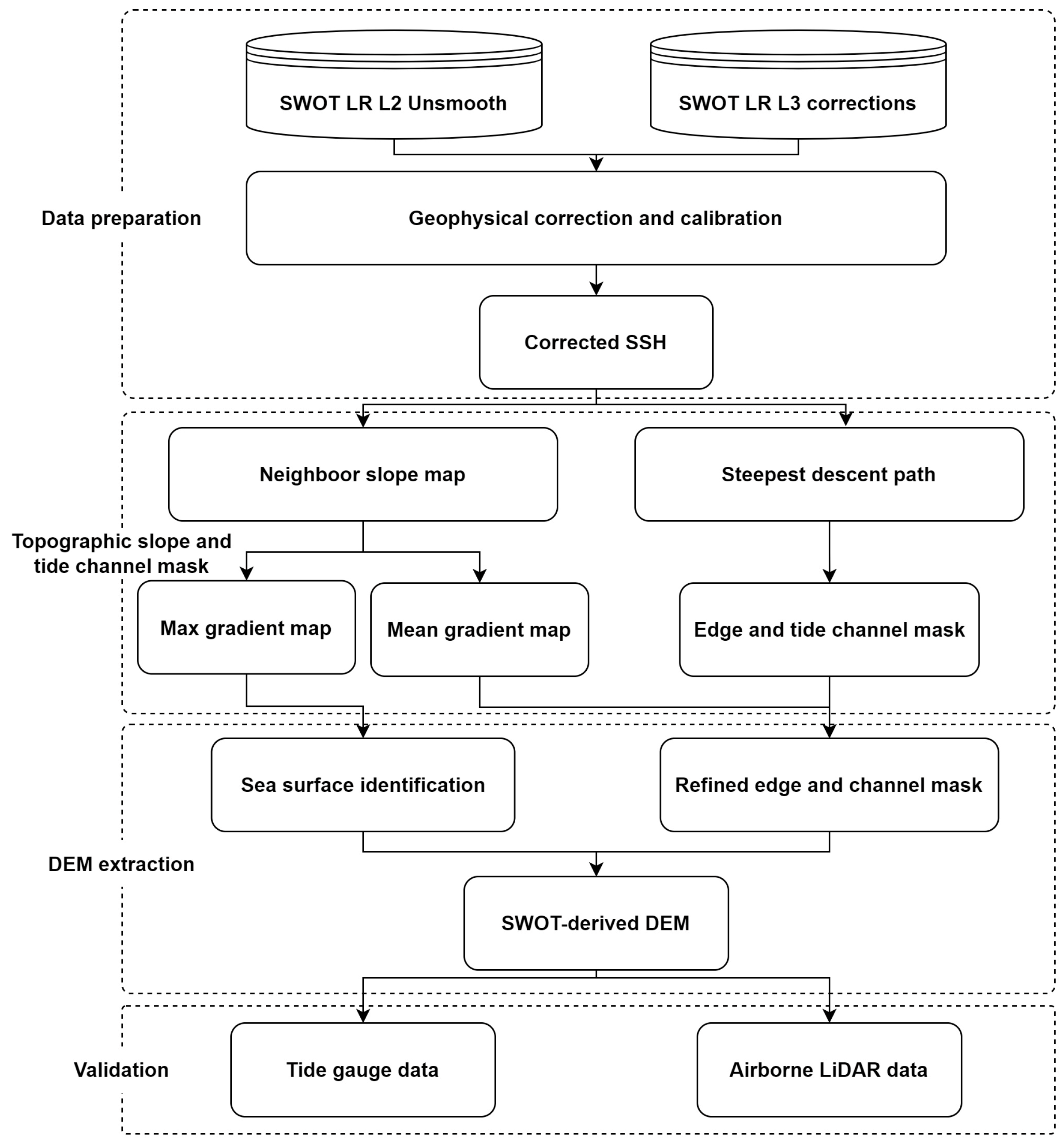
To independently validate the SWOT-derived DEM results, airborne LiDAR data provided by Xu et al. (2022) are introduced [15]. The airborne LiDAR data, indicated by a purple rectangle in Figure 1b, were collected in July 2019 over a 3 × 3 km coastal zone (120.97°E–121.00°E, 32.835°N–32.855°N), with a spatial resolution of 1 × 1 m and height accuracy reaching the centimeter level [15]. The topographic features acquired by LiDAR data are illustrated in Figure 2.

3. Methodology

This study proposes a framework for intertidal DEM information extraction using SWOT LR unsmoothed products. The process mainly includes data correction and preprocessing, topographic slope map construction, and tide channel masking. First, geophysical correction and systematic error correction parameters are applied to correct the original sea surface height anomalies (SSHA). Subsequently, an eight-neighborhood slope operator is employed to calculate topographic slope maps. Leveraging the bimodal histogram characteristics of the maximum gradient field, an adaptive threshold for distinguishing between sea and land is determined, which facilitates the separation of sea and land elevations. To further refine the results, an adaptive neighborhood steepest descent algorithm is introduced to generate a tidal channel mask. After morphological optimization, the intertidal DEM signals are extracted from the SWOT data. The accuracy of SWOT data for sea surface and land elevation measurements is then validated using tide gauge data and airborne LiDAR data, respectively. Detailed algorithm processing flow can be seen in Figure 3.

3.1. Data Preprocessing

Given the significant orbital, phase, and tilt errors present in the SSHA data of the SWOT L2 LR products, calibration information from the L3 product is used for correction [43,44]. Additionally, to facilitate the validation of SWOT altimetry results against tide gauge data, the geophysical corrections provided in the L2 product are applied to restore the SSH signal [45,46]

$$SS{H}_{lr}=SSH{A}_{lr}+\Delta G+\Delta C$$

(1)

where $SS{H}_{lr}$ represents the SSH derived from LR products, and $SSH{A}_{lr}$ represent the corresponding SSHA data; $\Delta G$ represents the geophysical corrections related to tides (including solid Earth and pole tides), and $\Delta C$ denotes the calibration information provided by the L3 product [47]. Considering that the vertical datum for LR products are based on CNES_CLS_2022 mean sea surface model (CLS22MSS) and earth gravitational model 2008 (EGM08), respectively [48,49], this study unifies the vertical datums of the tide gauge data and $SS{H}_{lr}$ to the CLS22MSS for better comparison.

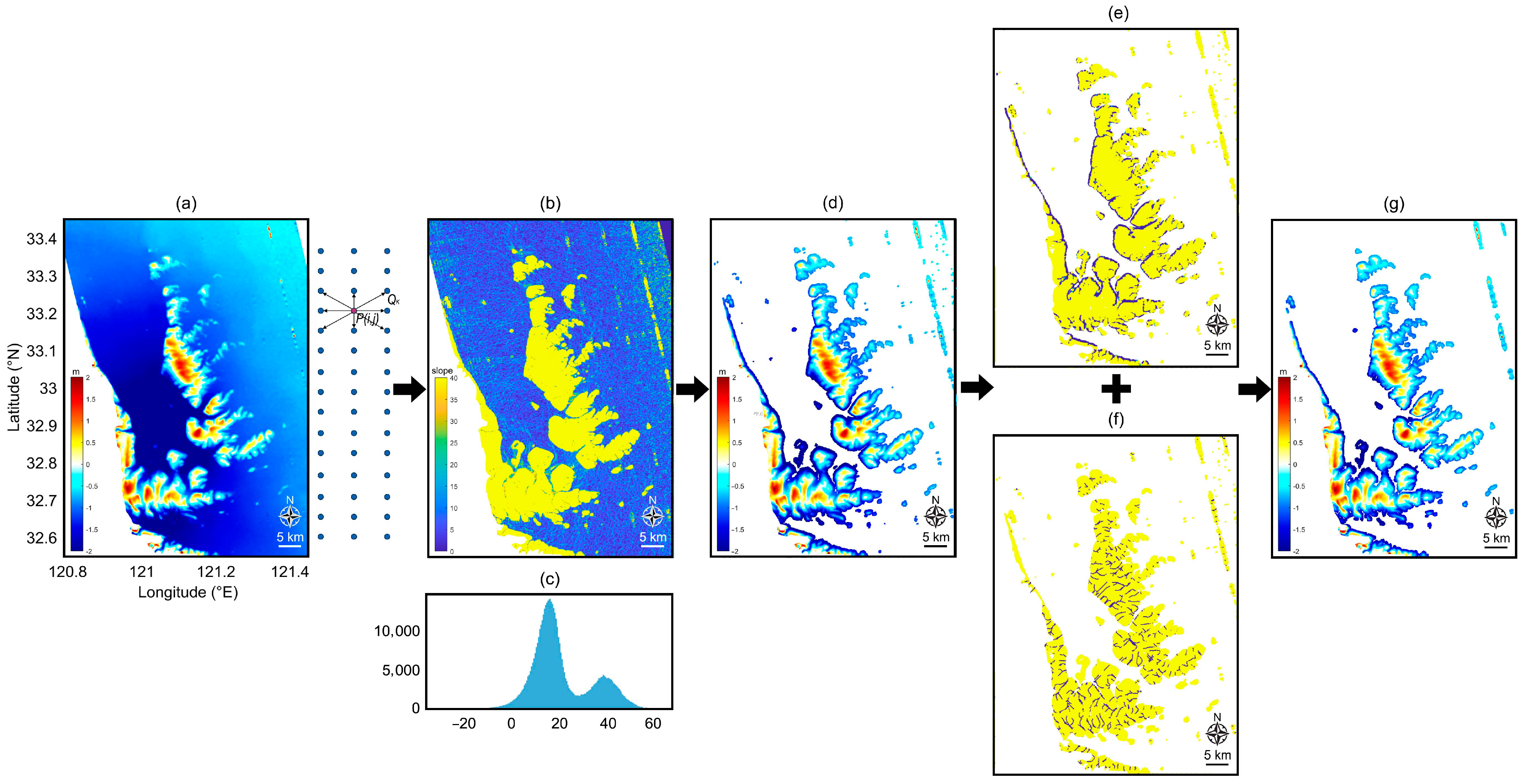
3.2. Slope Map and Tide Channel Mask

3.2.1. Topographic Slope Map Construction

The topographic slope is a crucial parameter for characterizing the variability of topography and can reveal subtle local changes. Considering that sea surface is a spatially continuous and smoothly varying surface, while intertidal topography exhibit more abrupt variations, a neighborhood gradient operator is employed to help distinguishing between sea surface and topography signals. For each point $P(i,j)$ in the SWOT data, multi-directional slope calculations are performed. Starting from the north direction, the slope values between the target point $P(i,j)$ and its eight neighboring points $Q_k(k\in \left\{1,2,\cdots ,8\right\})$ are computed in a clockwise manner (as shown in the right panel of Figure 4a). A three-dimensional table $G\left(i,j,k\right)$ that represents the topological relationship between the LR data and its neighbors is established to record the slope information. The elements of $G\left(i,j,k\right)$ are defined as the elevation slopes between $P(i,j)$ and its neighboring point $Q_k$

$$G(i,j,k)={\displaystyle \frac{h_{Q_k}-h_{i,j}}{d_{i,j,k}}}$$

(2)

where $h_{i,j}$ and $h_{Q_k}$ denote the elevation of $P(i,j)$ and $Q_k$, respectively, $d_{i,j,k}$ is the arc length calculated based on the WGS-84 ellipsoid between two points.

In order to better conduct land–water separation, the maximum slope map $G_{\max }$ and average slope map $G_{avg}$ are constructed based on $G\left(i,j,k\right)$

$$\begin{array}{l}{G}_{\max }(i,j)=\underset{1\le k\le 8}{\max }(G(i,j,k))\\ G_{avg}(i,j)={\displaystyle \frac{1}{8}}{\displaystyle \sum _{k=1}^{8}G}(i,j,k)\end{array}$$

(3)

3.2.2. Tidal Channel Masking

Considering the extensive distribution of tidal channels that are intermittently submerged at different tidal stages, it is necessary to remove them during the DEM extraction. This study applies a steepest descent path algorithm to iteratively identify local minima within the slope map, generating a tidal channel mask that delineates terrain concavities [50]. A counter table $C_{i,j}$ is initialized to track the frequency at which each point is visited during the tidal channel identification process. Points with higher visit frequencies are more likely to be part of a tidal channel. The steepest descent path follows the direction of the maximum downslope gradient, for each $P(i,j)$, the direction is determined

$$\underset{k}{Dir(i,j)=\arg \min (G(i,j,k))}$$

(4)

The steepest descent path is tracked iteratively, recording the number of times each point is visited. Specifically, at each step, if the elevation of a neighborhood point $Q_k$ is lower than that of the current point $P(i,j)$, the search continues in that direction until no further descent is possible. Finally, tidal channel lines are extracted based on the counter matrix and a predefined threshold ($g_0$)

$$M_{channel}(i,j)=\{(i,j)\mid C(i,j)\ge g_0\}$$

(5)

where $g_0$ is set to 40 based on empirical testing.

3.3. DEM Extraction

Taking the LR data from 7 September 2023 as an example (Figure 4), Figure 4a illustrates the raw SWOT data in the research area, the sea surface in the study area exhibits an irregular topography, making it challenging to eliminate sea surface signals using a fixed elevation threshold. However, given the differences in slope characteristics between land and sea surfaces, a preliminary DEM mask is constructed based on the histogram analysis of $G_{\max }(i,j)$ (Equation (3)). The distribution of the $G_{\max }(i,j)$, as illustrated in Figure 4b, effectively captures the pronounced variability of land surface. The corresponding histogram in Figure 4c reveals a bimodal distribution. By identifying the valley between the two peaks, a water–land separation threshold ($p_v$) is determined. To mitigate misclassification in low-relief areas due to $p_v$, tide gauge data ($h_{tide}$) are incorporated as an absolute reference for DEM mask construction ($M_{dem}$)

$$M_{dem}\left(i,j\right)=\left\{G\left(i, j\right)>p_v\cup SSH\left(i, j\right)>1.5\cdot h_{tide}\right\}$$

(6)

$$p_v=\arg \underset{i}{\min }\left(p_i\mid p_i<p_{i-1}\cap p_i<p_{i+1}\right)$$

(7)

As shown in Figure 4d, a preliminary DEM is extracted based on $M_{dem}\left(i,j\right)$. To address the misclassification issue occurs in coastal transition zones and tidal channel regions, an additional mask $M_{edge}$ is constructed by integrating the mean gradient ($G_{avg}$) and the tidal channel mask ($M_{channel}$). Moreover, a 2 × 2 median filter is applied to $G_{avg}$ to mitigate the pepper noise.

Figure 4e,f present the $G_{avg}$ and $M_{channel}$, respectively. The resulting mean slope map effectively enhances edge features at the land–sea interface.

$$M_{edge}(i,j)=(G_{avg}^{filter}(i,j)>T\cup M_{channel}(i,j))$$

(8)

The rasterized DEM mask $M_{dem}\left(i,j\right)$ is then subjected to a morphological dilation operation using a 4 × 4 kernel, followed by a 2 × 2 erosion. This process is intended to smooth the mask boundaries while preserving valid regions. Subsequently, connected component analysis was conducted, and regions smaller than 50 pixels in the study area are removed, effectively eliminating erroneous masks caused by noise interference. The DEM is then extracted based on the $M_{dem}$ and tidal channel/boundary masks $M_{edge}$

$$M_{dem}^{refine}(i,j)=M_{dem}(i,j)-M_{edge}(i,j)$$

(9)

As shown in Figure 4g, the framework proposed in this study effectively extracts DEM information from SWOT data and refines the masks for land–sea interface areas and tidal channels.

3.4. Vertical Accuracy Evaluation

Since SWOT data are the first altimeter capable of providing wide-swath measurements of both sea surface and land elevation, it is necessary to separately evaluate the accuracy of these measurements, considering the differences in radiometric properties between water and land surfaces. This study introduces tide gauge data and airborne LiDAR data to validate the altimetric accuracy of SWOT data.

Data from three nearby tide gauges (i.e., Dafeng, Yanghe, and Gensha) are obtained and interpolated to the SWOT overpass times using the nearest neighbor method. The instantaneous SSH derived from SWOT at each tide gauge station is calculated by averaging the SSHs within a 1 km radius around the gauge stations. Similarly, the DEM data obtained from airborne LiDAR is interpolated to the SWOT grid points for point-by-point validation. It is important to note that due to the high temporal resolution (10 min) of the tide gauge data and the high spatial resolution (1 m) of the LiDAR data, the interpolation errors when performing temporal and spatial interpolations are on the order of 0.01 m, which is significantly smaller than the observation errors. Therefore, the impact of interpolation errors is negligible in this study.

The differences between the SSH obtained from SWOT and tide gauge data ($\Delta h_{SSH}$), as well as the differences between the SWOT-derived DEM and airborne LiDAR data ($\Delta h_{DEM}$), can be expressed as

$$\begin{array}{l}\Delta h_{SSH}=SS{H}_{lr}-h_{tide},\\ \Delta h_{DEM}=DE{M}_{lr}-h_{lidar}\end{array}$$

(10)

where $SS{H}_{lr}$ and $DE{M}_{lr}$ represent the SSH and land elevation derived from SWOT LR data, respectively, and $h_{tide}$ and $h_{lidar}$ represent the tidal level measured by the tide gauge and land elevation obtained from airborne LiDAR, respectively.

The root mean square error (RMSE) metric is employed to indicate the vertical accuracy of SWOT measurements

$$RMS{E}_{\Delta h}=\sqrt{{\displaystyle \frac{1}{n}}{\displaystyle \sum _1^n\Delta h_i^2}}$$

(11)

where $RMS{E}_{\Delta h}$ represents the RMSE value for $\Delta h_{SSH}$ or $\Delta h_{DEM}$, $n$ and $i$ represent the total number and the index of sampling points, respectively.

4. Results

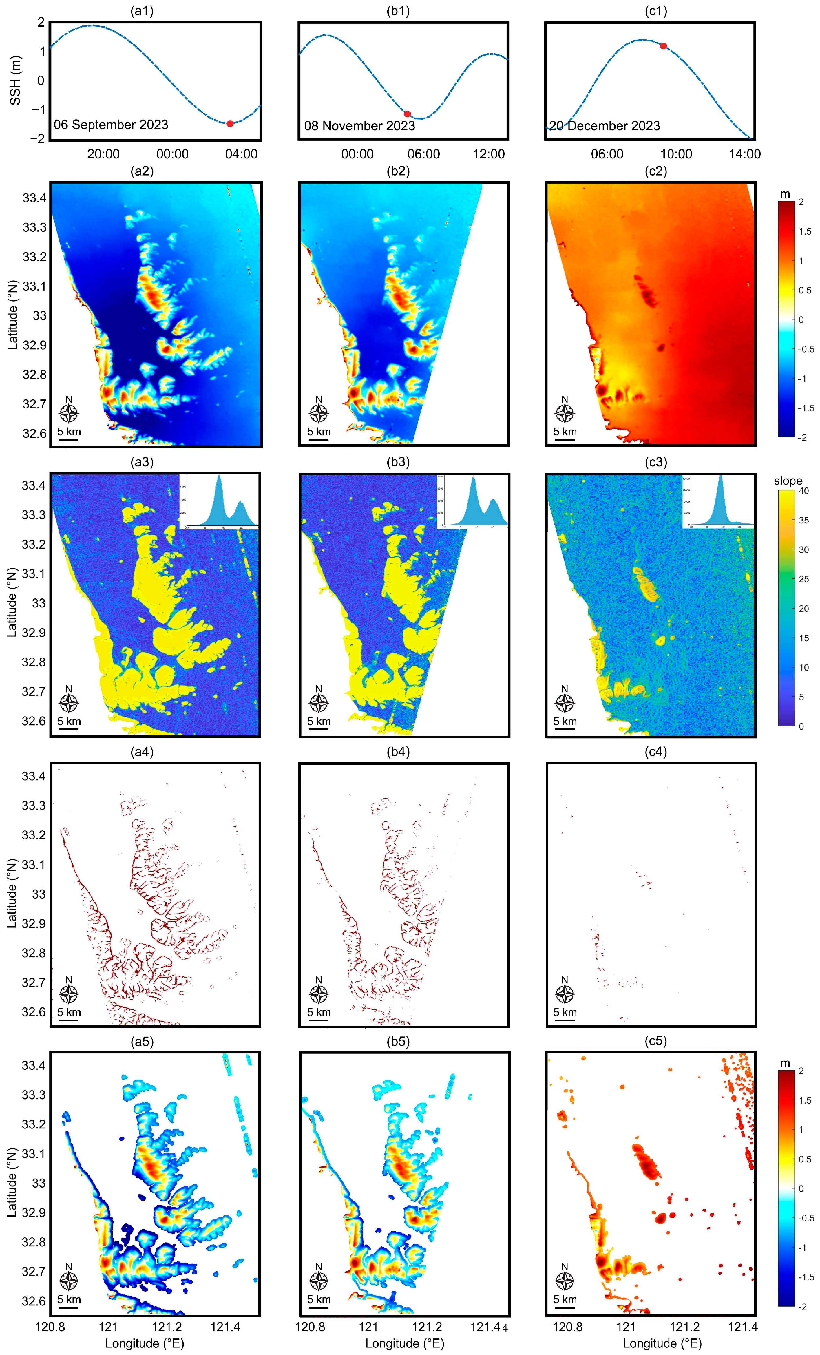
4.1. DEM Results from SWOT

Fifty tracks of LR products from July 2023 to December 2024 are utilized to extract DEM information in the intertidal area of Jiangsu. To verify the effectiveness of the proposed algorithm for DEM extraction from SWOT data, three typical tracks at different tidal stage (i.e., tracks from 6 September, 8 November, and 20 December 2023) were selected to illustrate the data processing procedures and results. As shown in Figure 5, each row represents different types of analysis results: the first row provides the tide level during the SWOT overpass over the study area; the second row displays the SWOT SSH data; the third row shows the maximum slope map and its distribution histogram; the fourth row presents tide channel and land–water boundary masks; and the fifth row exhibits the extracted DEM results. Each column represents data from different time points: the first column from 6 September 2023; the second from 8 November 2023; and the third from 20 December 2023. Based on the tide series in the first row of Figure 5, the tidal range in the study area varies between ±2 m, with the three typical SWOT tracks corresponding to tidal levels of −1.1 m, −0.7 m, and 0.9 m. The second row of SWOT data illustrates the spatial distribution of SSH under different tide levels and the changes in the inundated area of the intertidal DEM. For example, during a low tide stage on 6 September 2023, the DEM’s inundated area was relatively small. In contrast, during a higher tide stage on 20 December 2023, over 80% of the tidal flat was submerged.

As shown in the second row of Figure 5, the LR data indicate significant spatial variations in SSH within the study area. For instance, the SSH in Figure 5(a2) is approximately −2 m near the coastline (121°E, 32.9°N), whereas it increases to 0.5 m at (122°E, 32.8°N). This demonstrates that the sea surface within the study area exhibits an irregular topography, making it challenging to extract DEM signals through surface fitting or elevation thresholding. However, the slope maps in the third row (e.g., Figure 5(a3)) show greater topographic variability over land than sea, enabling a clear distinction between water bodies and land. The gradient histograms in the subplots display two distinct peaks for land and sea under different tidal conditions. Setting the gradient threshold at the valley between these peaks facilitates accurate DEM signal extraction. The land–water boundary and tide channel masks in the fourth row further refined the DEM signal extraction results. By comparing the results in the second and fifth rows, it is evident that the proposed algorithm achieves effective DEM extraction for LR data. The DEM results across three tidal stages reveal a consistent distribution pattern, with the inundation extent of the tidal flats expanding as the tidal level rises. This highlights the advantage of SWOT in capturing instantaneous, full-swath elevation data. However, it is also observed that LR data exhibit striping artifacts at the swath boundaries.

This study employs tidal variation analysis to identify SWOT observations corresponding to low-tide periods, thereby maximizing the extraction of tidal flat morphology and ensuring the spatial continuity of the resulting DEM. The tide gauge data from July 2023 to December 2024 at Dafeng Station, shown in Figure 6, reveal significant tidal variations within the study area, with a maximum tidal range exceeding 5 m. Specifically, the highest tide reached 2.4 m on 5 August 2024, while the lowest tide fell to −2.8 m on 12 March 2024. Therefore, the SWOT data from the lowest tide level (7 October 2024, with an SSH of −1.99 m) is selected for DEM analysis. Figure 7a illustrates the DEM results based on LR data, along with the local magnified view in Figure 7b. It shows that the intertidal DEM in this region ranges about ±2 m. Specifically, the maximum elevations in the Tiaozini, Gensha, and Dongsha areas are 2.3 m (32.74°N, 121.03°E), 2.1 m (32.88°N, 121.15°E), and 1.89 m (33.5°N, 121.11°E), respectively. The magnified views reveal more detailed DEM features, particularly in the Tiaozini area. The elevation distribution shows a gradual decrease from 32.717°N towards both sides, highlighting isolated hilltops and gullies formed by tidal effects. These characteristics indicate that the intertidal terrain has been shaped through erosion and deposition processes. The periodic rise and fall of tides endow the topography of this region with significant spatiotemporal variability.

To further evaluate the performance of the tidal channel mask, a DEM profile along 32.72°N (green dashed line in Figure 7b) crossing a typical geomorphological area of Tiaozini was extracted. Figure 8a,b present the DEM profiles obtained without and with the application of the tidal channel mask, respectively. In the regions near 121.00°E and 121.05°E, which are influenced by tidal inundation, the DEM signals display significant temporal variability. The tidal channel mask effectively identifies and removes the tide signals from the DEM data (Figure 8b), thereby improving the accuracy and reliability of the DEM. Additionally, in the region near 121.03°E, it is evident that this area is rarely submerged by seawater, leading to high consistency in the DEM signal patterns derived from different datasets.

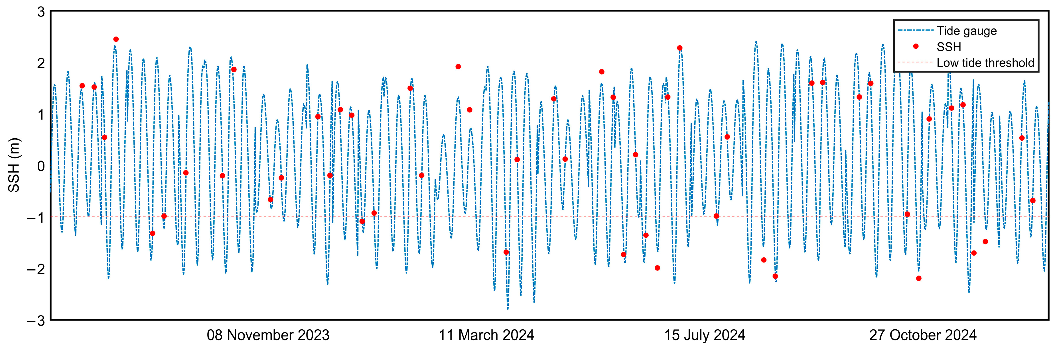
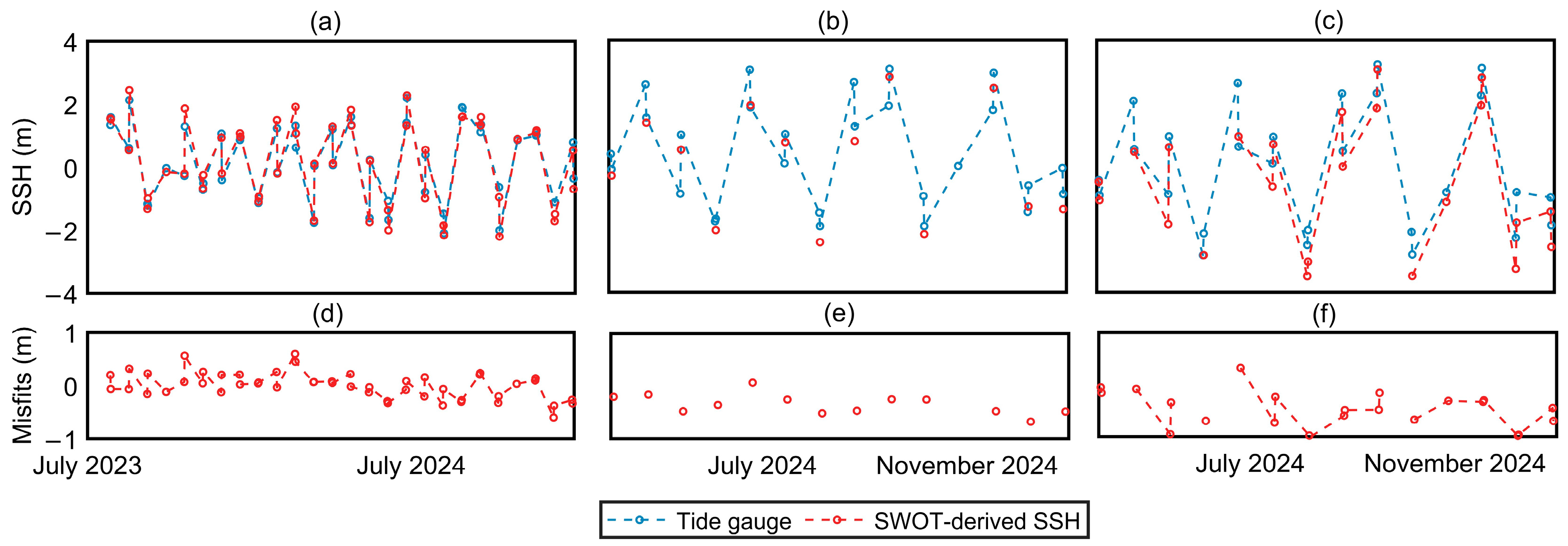
4.2. Validation of SWOT-Derived SSH and DEM

The LR sea surface and land altimetry accuracy are evaluated using tide gauge data and airborne LiDAR data, respectively. Figure 9 shows the SSH validation results for LR data against three tide gauges, with detailed statistics provided in

Table 1. Statistics of the SSH validation results using tide gauge data (m).

Tide Stations	Max	Min	Mean	RMSE
Dafeng	0.59	−0.60	0.01	0.25
Gensha	0.26	−0.47	−0.16	0.19
Yanghe	0.62	−0.70	−0.19	0.32

.

The results indicate that the SWOT-derived SSH is highly consistent with the tide gauge data, showing robust performance, especially in the coastal region. Specifically, the RMSE of the validation results for Gensha Station is 0.19 m, which is lower than that for the Dafeng Station (0.25 m) and Yanghe Station (0.32 m). This may be attributed to the relatively stable sea surface variations in open waters, whereas coastal areas are subject to more pronounced spatial changes due to the influence of land and seafloor topography. Additionally, the lower spatial resolution and accuracy of ionospheric and tropospheric models in coastal regions may affect SWOT performance. The shorter data collection period at the Gensha gauge compared to the Dafeng gauge may also contribute to differences in the statistical results.

Given the significant differences in backscattering characteristics and topographic variability between oceanic and terrestrial surfaces, validation based solely on tide gauge data may not accurately reflect the land altimetry accuracy of SWOT. Thus, the airborne LiDAR data are employed to provide a more comprehensive evaluation of the SWOT-derived DEM [15]. Figure 10 illustrates Figure 10a the distribution of airborne LiDAR data and LR data, Figure 10b the difference map between them, and Figure 10c the results of the regression analysis. Results indicate that the SWOT-derived DEM exhibits high consistency in the region between 120.97°E and 120.98°E, with an average difference of only 0.05 m. However, in the land–sea boundary areas (e.g., 32.84°N, 120.99°E) and tidal channel regions (e.g., 32.85°N, 120.98°E), the misfits increase significantly (exceeding 0.5 m). This discrepancy can be attributed to two main factors. First, the airborne data were collected in July 2019, approximately five years prior to the SWOT data (October 2024). The intertidal topography experiences significant spatiotemporal changes due to tidal inundation over the five years, leading to variations in the land–sea boundary and tidal channels, while areas less affected by tidal erosion remain relatively stable. Second, the spatial resolution of the LR data is approximately 250 m, which limits the ability to resolve narrow tidal channels and consequently affects the accuracy in these regions. Regression analysis reveals that the SWOT-derived DEM and LiDAR data exhibit good consistency within the 0–1 m elevation range, while it deteriorates in the land–sea boundary zone between −0.5 m and 0 m. Statistically, the validation results yield an RMSE of 0.24 m, with a maximum of 0.89 m, a minimum of −0.79 m, and a mean of 0.05 m.

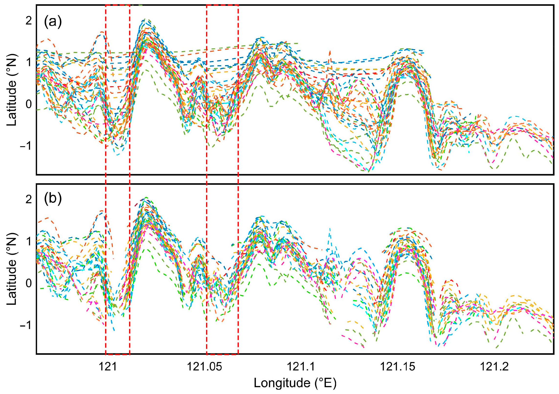
4.3. Spatiotemporal Variation Analysis

Leveraging the wide-swath coverage capability of SWOT, DEM extraction was performed based on 50 tracks acquired from July 2023 to December 2024, enabling time-varying analysis of intertidal topographic changes. This study set a low tide threshold of -1.05 m (Figure 6 red dashed line) and selected 12 tracks (from September 2023 to December 2024) below this threshold for temporal analysis over a 16-month period. Figure 11 illustrates the SD (Standard Deviation) distribution of elevation for each point. By excluding tidal channels and land–water boundary signals, Figure 11 primarily highlights the extent of terrain changes within the time span. It is evident that the most significant changes are concentrated in the Southern Zhugensha and Northern Tiaozini areas (over 0.5 m), while the Dongsha area shows minimal elevation changes (~0.1 m). The magnified view on the right side of Figure 11 reveals that changes in Zhugensha and Tiaozini are mainly concentrated in low-elevation land–sea boundary areas and tidal channels. These changes can be attributed to both terrain alterations and residual sea surface signal interference. Comparing the Dongsha and Tiaozini areas, it is clear that tidal erosion is the primary driver of significant elevation changes in Tiaozini. Furthermore, due to the northern part of Tiaozini being exposed to incoming water, the ocean dynamic effects in this region are more pronounced, leading to substantial topographic changes compared to other areas [41]. However, in higher elevation areas (e.g., 32.74°N, 121.02°E and 32.88°N, 121.15°E), which are rarely submerged by seawater, elevation changes are minimal. It should be noted that given the altimetry accuracy of SWOT data is ~0.3 m in the study area (Figure 10), the magnitude of these topographic variations may be overestimated. Nonetheless, it still demonstrates the capability of SWOT data for monitoring temporal variations in the intertidal area. Furthermore, as shown in Figure 12, Pearson correlation analysis of these 12 DEM datasets indicates a negative correlation trend with time [51]. For instance, the DEM data from 6 September 2023 have a correlation coefficient of 0.94 with data from 9 January 2024, which gradually decreases to 0.84 by 9 December 2024. This finding highlights the strong temporal variability of the intertidal topography, reflecting the continuous impact of marine dynamic processes on intertidal terrain.

5. Discussion

To further evaluate the topographic changes in the Tiaozini area and the ability of SWOT data in capturing detailed surface features, the SWOT-derived DEMs from 7 September 2023, and 9 December 2024, were compared, and Sentinel-2 imagery (on 20 October 2023 and 17 January 2025) closest in time to these two datasets was obtained for corroboration. As shown in Figure 13a,b, the two SWOT datasets reveal significant changes in the topographic features of the Tiaozini area, particularly in the tidal channels and coastal regions (marked by red and green boxes in Figure 13). These changes are consistent with the signal patterns observed in the Sentinel-2 imagery from Figure 13c,d. These are primarily attributed to erosion caused by tidal inundation and recession. Also, the Sentinel-2 imagery reveals a clear coastal current between Tiaozini and Zhugensha, which intensifies seawater scouring and accelerates topographic changes in the area. Furthermore, the two SWOT tracks, separated by 16 months, indicate dynamic changes in the tidal channels within the Tiaozini region. Overlaying the main channels extracted from SWOT data onto the corresponding imagery (black curves in Figure 13), it is observed that the shapes and trajectories of the extracted river channels align well with those in the imagery. The topographic features captured by SWOT are consistent with the patterns observed in the remote sensing imagery, demonstrating SWOT’s robust capability for DEM signal extraction.

The aforementioned results highlight that the intertidal zone experiences pronounced spatiotemporal topographic changes due to tidal erosion. Traditional algorithms based on remote sensing imagery rely on long-term accumulation of imagery and tidal data, making it challenging to efficiently monitor time-varying topographic signals. In contrast, SWOT’s wide-swath interferometric measurement technology enables the monitoring of sea surface and land elevation across a 120 km wide swath in a single observation, significantly enhancing data quality and temporal resolution in intertidal areas.

Nevertheless, a more comprehensive evaluation is required to fully characterize the quality of SWOT-derived DEMs. Although this study focused on absolute vertical accuracy due to limitations in large-scale in situ data and the lack of temporally synchronized high-resolution remote sensing imagery, other critical factors, such as relative vertical accuracy and surface accuracy, are essential for a thorough DEM assessment [52,53,54]. Specifically, the relative vertical accuracy ensures precise calculations of terrain derivatives like slope, aspect, and curvature, which are crucial for research in geomorphology and oceanography [55]. Simultaneously, the surface accuracy reflects the completeness of feature representation (e.g., ridgelines), determining the DEM’s capacity to preserve terrain structural integrity [54,56]. Future work will integrate more large-scale airborne LiDAR products and multi-source remote sensing datasets to establish a comprehensive evaluation framework. By addressing these aspects, the reliability and applicability of SWOT-derived DEMs in various scientific domains, including geology, oceanography, and environmental management, will be significantly enhanced.

6. Conclusions

Accurate intertidal topographic information is of significant importance for coastal ecological conservation, coastline erosion monitoring, and global climate change assessment. This study proposes a framework for extracting intertidal DEMs from SWOT wide-swath altimetry data through three modules: data preprocessing, topographic gradient field construction, and land mask generation, enabling high-precision and high spatiotemporal resolution monitoring of intertidal topographic changes. Utilizing 50 tracks of SWOT L2 LR unsmoothed data from July 2023 to December 2024, this study achieved high-precision DEM extraction in the radial sand ridge area along the Jiangsu coast. Independent tide gauge and airborne LiDAR data were introduced to comprehensively evaluate the reliability of the DEM signals extracted by the proposed algorithm, as well as the sea surface and land altimetry accuracies of the LR products. Additionally, the spatiotemporal variations of intertidal topography were analyzed. The numerical results demonstrate the following:

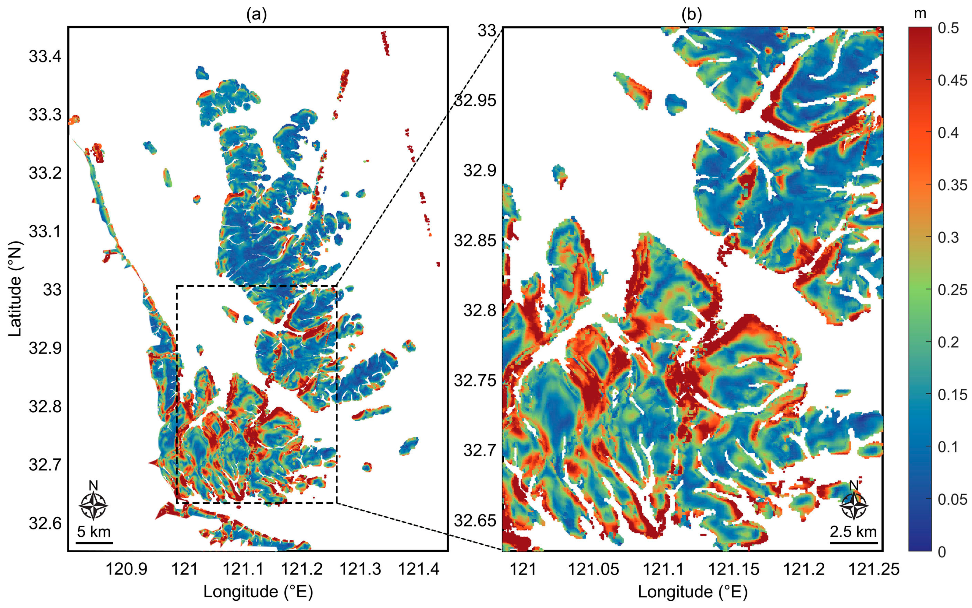
• The proposed algorithm achieves high-precision DEM extraction by effectively removing ocean signals using the slope map and tidal channel mask. In addition, the topographic features captured by the LR products are consistent with the patterns observed in the remote sensing imagery.
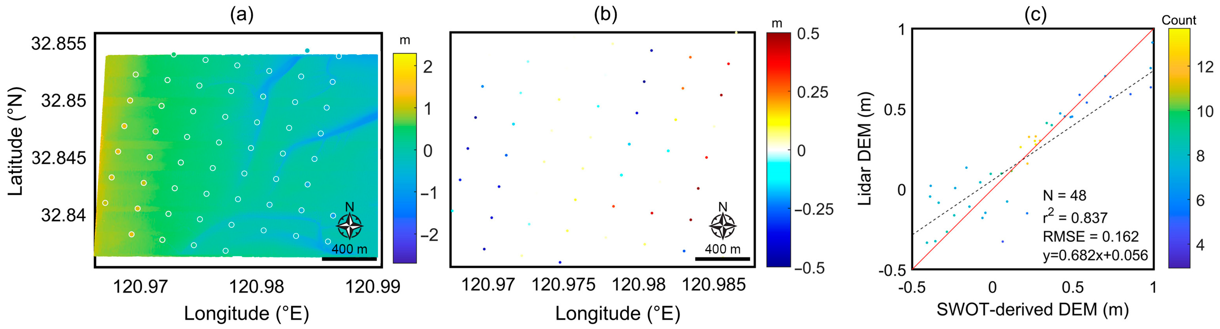
• Validation results based on tide gauge data show that SWOT data exhibit comparable SSH altimetry accuracy in coastal and open ocean areas. Specifically, the RMSE of the difference between SSH and tide data in Dafeng station is 0.25 m, 0.19 m at Yanghe station, and 0.32 m at the Gensha station. Regarding land altimetry accuracy, validation results based on LiDAR data indicate an RMSE of 0.24 m, confirming their reliability in intertidal topographic extraction.
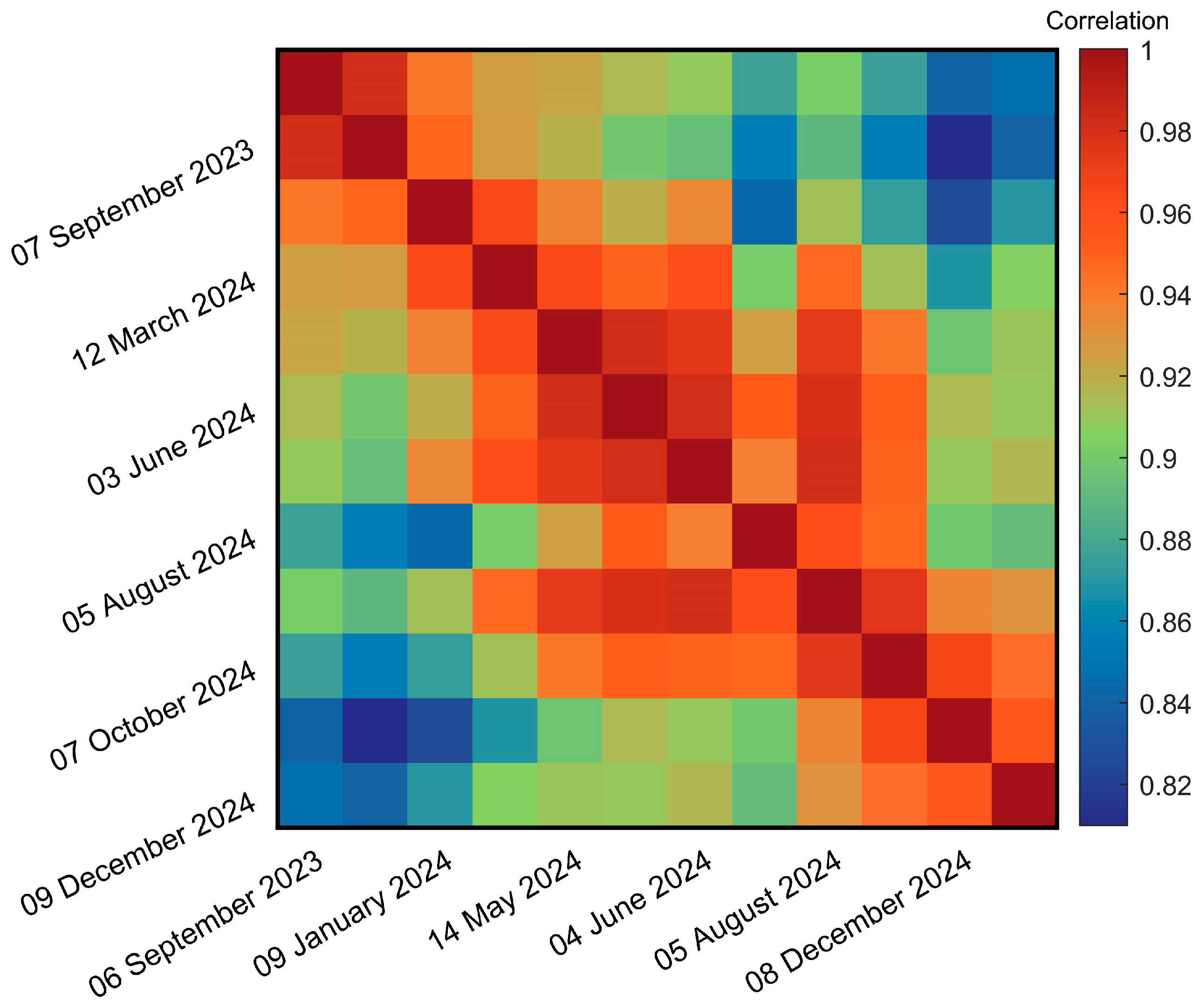
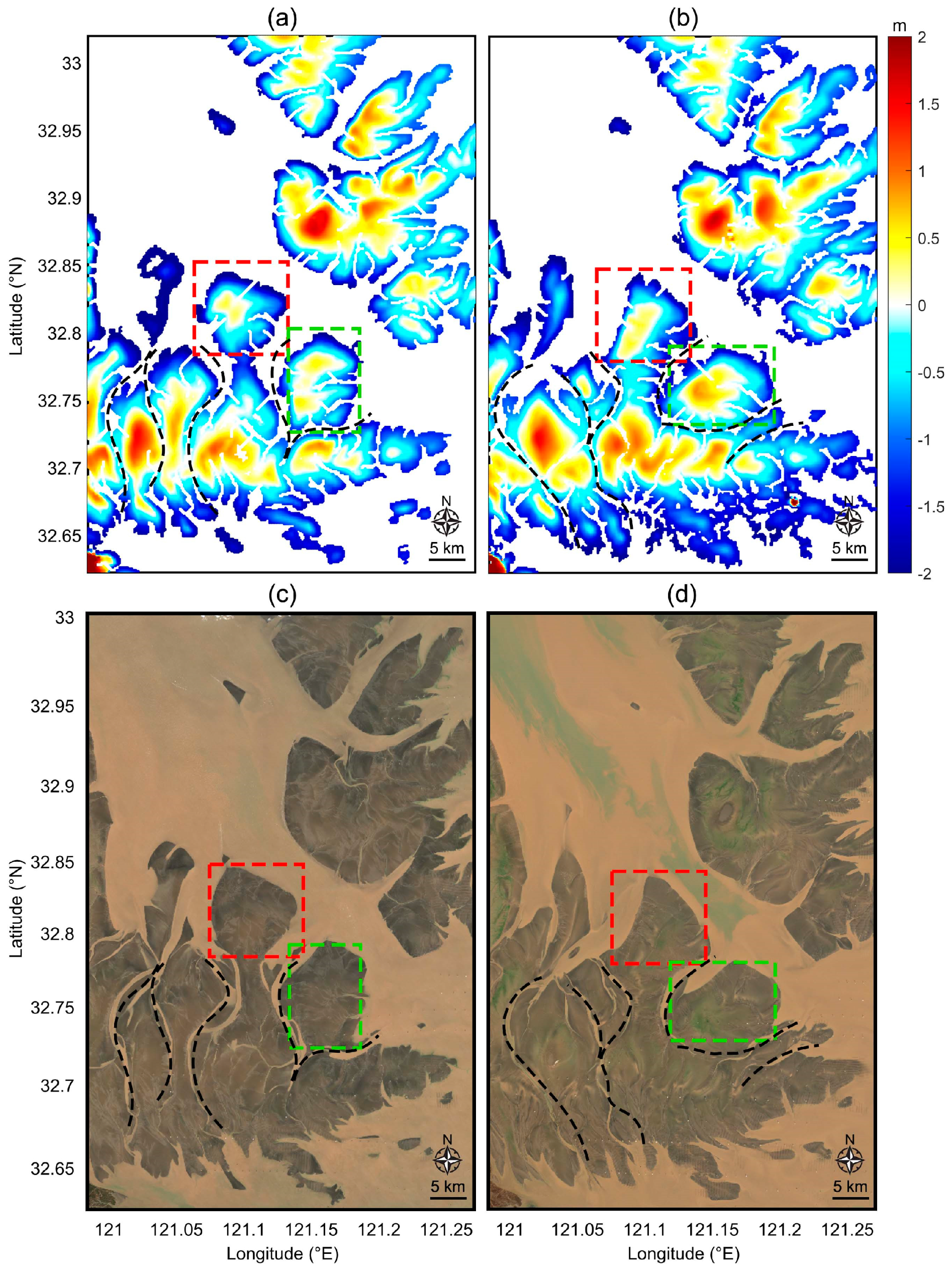
• SWOT data can provide high spatiotemporal resolution intertidal DEM information, enabling the analysis of spatiotemporal topographic variations. Based on a 16-month time series analysis of SWOT data, significant spatiotemporal changes were observed in the Tiaozini area, primarily concentrated in the land–sea boundary and tidal channel regions. The Pearson correlation of SWOT-derived DEMs decreases from 0.94 for a one-month time interval to 0.84 for a sixteen-month interval, reflecting the continuous impact of marine dynamic processes on intertidal topography. This suggests that traditional DEM construction methods relying on long-term data accumulation are prone to losing time-varying signals.

References

1. Ma, Z.; Li, B. Complex Ecology of China’s Seawall—Response. Science 2015, 347, 1080. [Google Scholar] [CrossRef]
2. Brand, E.; Chen, M.; Montreuil, A.-L. Optimizing Measurements of Sediment Transport in the Intertidal Zone. Earth Sci. Rev. 2020, 200, 103029. [Google Scholar] [CrossRef]
3. Helmuth, B.S.; Hofmann, G.E. Microhabitats, Thermal Heterogeneity, and Patterns of Physiological Stress in the Rocky Intertidal Zone. Biol. Bull. 2001, 201, 374–384. [Google Scholar] [CrossRef]
4. Mortimer, R.; Krom, M.; Watson, P.; Frickers, P.; Davey, J.; Clifton, R. Sediment–Water Exchange of Nutrients in the Intertidal Zone of the Humber Estuary, UK. Mar. Pollut. Bull. 1999, 37, 261–279. [Google Scholar] [CrossRef]
5. Widdows, J.; Brown, S.; Brinsley, M.; Salkeld, P.; Elliott, M. Temporal Changes in Intertidal Sediment Erodability: Influence of Biological and Climatic Factors. Cont. Shelf Res. 2000, 20, 1275–1289. [Google Scholar] [CrossRef]
6. Poulin, R.; Mouritsen, K.N. Climate Change, Parasitism and the Structure of Intertidal Ecosystems. J. Helminthol. 2006, 80, 183–191. [Google Scholar] [CrossRef]
7. Jin, H.; Huang, C.; Lang, M.W.; Yeo, I.-Y.; Stehman, S.V. Monitoring of Wetland Inundation Dynamics in the Delmarva Peninsula Using Landsat Time-Series Imagery from 1985 to 2011. Remote Sens. Environ. 2017, 190, 26–41. [Google Scholar] [CrossRef]
8. Murray, N.J.; Phinn, S.R.; DeWitt, M.; Ferrari, R.; Johnston, R.; Lyons, M.B.; Clinton, N.; Thau, D.; Fuller, R.A. The Global Distribution and Trajectory of Tidal Flats. Nature 2019, 565, 222–225. [Google Scholar] [CrossRef]
9. Fitton, J.M.; Rennie, A.F.; Hansom, J.D.; Muir, F.M. Remotely Sensed Mapping of the Intertidal Zone: A Sentinel-2 and Google Earth Engine Methodology. Remote Sens. Appl. Soc. Environ. 2021, 22, 100499. [Google Scholar] [CrossRef]
10. Bishop-Taylor, R.; Sagar, S.; Lymburner, L.; Beaman, R.J. Between the Tides: Modelling the Elevation of Australia’s Exposed Intertidal Zone at Continental Scale. Estuar. Coast. Shelf Sci. 2019, 223, 115–128. [Google Scholar] [CrossRef]
11. Zhang, L.; Li, N.; Jia, S.; Wang, T.; Dong, J. A Method for DEM Construction Considering the Features in Intertidal Zones. Mar. Geod. 2015, 38, 163–175. [Google Scholar] [CrossRef]
12. Mason, D.; Scott, T.; Dance, S. Remote Sensing of Intertidal Morphological Change in Morecambe Bay, UK, between 1991 and 2007. Estuar. Coast. Shelf Sci. 2010, 87, 487–496. [Google Scholar] [CrossRef]
13. Andriolo, U.; Almeida, L.P.; Almar, R. Coupling Terrestrial LiDAR and Video Imagery to Perform 3D Intertidal Beach Topography. Coast. Eng. 2018, 140, 232–239. [Google Scholar] [CrossRef]
14. Enwright, N.M.; Wang, L.; Borchert, S.M.; Day, R.H.; Feher, L.C.; Osland, M.J. The Impact of Lidar Elevation Uncertainty on Mapping Intertidal Habitats on Barrier Islands. Remote Sens. 2017, 10, 5. [Google Scholar] [CrossRef]
15. Xu, N.; Ma, Y.; Yang, J.; Wang, X.H.; Wang, Y.; Xu, R. Deriving Tidal Flat Topography Using ICESat-2 Laser Altimetry and Sentinel-2 Imagery. Geophys. Res. Lett. 2022, 49, e2021GL096813. [Google Scholar] [CrossRef]
16. Khan, M.J.U.; Ansary, M.N.; Durand, F.; Testut, L.; Ishaque, M.; Calmant, S.; Krien, Y.; Islam, A.K.M.S.; Papa, F. High-Resolution Intertidal Topography from Sentinel-2 Multi-Spectral Imagery: Synergy between Remote Sensing and Numerical Modeling. Remote Sens. 2019, 11, 2888. [Google Scholar] [CrossRef]
17. Ryu, J.-H.; Kim, C.-H.; Lee, Y.-K.; Won, J.-S.; Chun, S.-S.; Lee, S. Detecting the Intertidal Morphologic Change Using Satellite Data. Estuar. Coast. Shelf Sci. 2008, 78, 623–632. [Google Scholar] [CrossRef]
18. Ma, Y.; Xu, N.; Liu, Z.; Yang, B.; Yang, F.; Wang, X.H.; Li, S. Satellite-Derived Bathymetry Using the ICESat-2 Lidar and Sentinel-2 Imagery Datasets. Remote Sens. Environ. 2020, 250, 112047. [Google Scholar] [CrossRef]
19. Yang, F.; Qi, C.; Su, D.; Ding, S.; He, Y.; Ma, Y. An Airborne LiDAR Bathymetric Waveform Decomposition Method in Very Shallow Water: A Case Study around Yuanzhi Island in the South China Sea. Int. J. Appl. Earth Obs. Geoinf. 2022, 109, 102788. [Google Scholar] [CrossRef]
20. Monteys, X.; Harris, P.; Caloca, S.; Cahalane, C. Spatial Prediction of Coastal Bathymetry Based on Multispectral Satellite Imagery and Multibeam Data. Remote Sens. 2015, 7, 13782–13806. [Google Scholar] [CrossRef]
21. Choi, C.; Kim, D. Optimum Baseline of a Single-Pass In-SAR System to Generate the Best DEM in Tidal Flats. IEEE J. Sel. Top. Appl. Earth Obs. Remote Sens. 2018, 11, 919–929. [Google Scholar] [CrossRef]
22. Wang, H.; Wright, T.J.; Yu, Y.; Lin, H.; Jiang, L.; Li, C.; Qiu, G. InSAR Reveals Coastal Subsidence in the Pearl River Delta, China. Geophys. J. Int. 2012, 191, 1119–1128. [Google Scholar] [CrossRef]
23. Li, P.; Wang, G.; Liang, C.; Wang, H.; Li, Z. InSAR-Derived Coastal Subsidence Reveals New Inundation Scenarios over the Yellow River Delta. IEEE J. Sel. Top. Appl. Earth Obs. Remote Sens. 2023, 16, 8431–8441. [Google Scholar] [CrossRef]
24. Yang, F.; Su, D.; Ma, Y.; Feng, C.; Yang, A.; Wang, M. Refraction Correction of Airborne LiDAR Bathymetry Based on Sea Surface Profile and Ray Tracing. IEEE Trans. Geosci. Remote Sens. 2017, 55, 6141–6149. [Google Scholar] [CrossRef]
25. Salameh, E.; Frappart, F.; Turki, I.; Laignel, B. Intertidal Topography Mapping Using the Waterline Method from Sentinel-1 &-2 Images: The Examples of Arcachon and Veys Bays in France. ISPRS J. Photogramm. Remote Sens. 2020, 163, 98–120. [Google Scholar] [CrossRef]
26. Caballero, I.; Stumpf, R.P. Confronting Turbidity, the Major Challenge for Satellite-Derived Coastal Bathymetry. Sci. Total Environ. 2023, 870, 161898. [Google Scholar] [CrossRef]
27. Casal, G.; Hedley, J.D.; Monteys, X.; Harris, P.; Cahalane, C.; McCarthy, T. Satellite-Derived Bathymetry in Optically Complex Waters Using a Model Inversion Approach and Sentinel-2 Data. Estuar. Coast. Shelf Sci. 2020, 241, 106814. [Google Scholar] [CrossRef]
28. Hsu, H.-J.; Huang, C.-Y.; Jasinski, M.; Li, Y.; Gao, H.; Yamanokuchi, T.; Wang, C.-G.; Chang, T.-M.; Ren, H.; Kuo, C.-Y.; et al. A Semi-Empirical Scheme for Bathymetric Mapping in Shallow Water by ICESat-2 and Sentinel-2: A Case Study in the South China Sea. ISPRS J. Photogramm. Remote Sens. 2021, 178, 1–19. [Google Scholar] [CrossRef]
29. Costa, B.; Battista, T.; Pittman, S. Comparative Evaluation of Airborne LiDAR and Ship-Based Multibeam SoNAR Bathymetry and Intensity for Mapping Coral Reef Ecosystems. Remote Sens. Environ. 2009, 113, 1082–1100. [Google Scholar] [CrossRef]
30. Tang, M.; Zhao, Q.; Pepe, A.; Devlin, A.T.; Falabella, F.; Yao, C.; Li, Z. Changes of Chinese Coastal Regions Induced by Land Reclamation as Revealed through TanDEM-X DEM and InSAR Analyses. Remote Sens. 2022, 14, 637. [Google Scholar] [CrossRef]
31. Fjortoft, R.; Gaudin, J.-M.; Pourthie, N.; Lalaurie, J.-C.; Mallet, A.; Nouvel, J.-F.; Martinot-Lagarde, J.; Oriot, H.; Borderies, P.; Ruiz, C.; et al. KaRIn on SWOT: Characteristics of Near-Nadir Ka-Band Interferometric SAR Imagery. IEEE Trans. Geosci. Remote Sensing 2014, 52, 2172–2185. [Google Scholar] [CrossRef]
32. Fu, L.; Pavelsky, T.; Cretaux, J.; Morrow, R.; Farrar, J.T.; Vaze, P.; Sengenes, P.; Vinogradova-Shiffer, N.; Sylvestre-Baron, A.; Picot, N.; et al. The Surface Water and Ocean Topography Mission: A Breakthrough in Radar Remote Sensing of the Ocean and Land Surface Water. Geophys. Res. Lett. 2024, 51, e2023GL107652. [Google Scholar] [CrossRef]
33. Hart-Davis, M.G.; Andersen, O.B.; Ray, R.D.; Zaron, E.D.; Schwatke, C.; Arildsen, R.L.; Dettmering, D.; Nielsen, K. Tides in Complex Coastal Regions: Early Case Studies from Wide-swath SWOT Measurements. Geophys. Res. Lett. 2024, 51, e2024GL109983. [Google Scholar] [CrossRef]
34. Ardhuin, F.; Molero, B.; Bohé, A.; Nouguier, F.; Collard, F.; Houghton, I.; Hay, A.; Legresy, B. Phase-resolved Swells across Ocean Basins in SWOT Altimetry Data: Revealing Centimeter-scale Wave Heights Including Coastal Reflection. Geophys. Res. Lett. 2024, 51, e2024GL109658. [Google Scholar] [CrossRef]
35. Zhang, H.; Fan, C.; Sun, L.; Meng, J. Study of the Ability of SWOT to Detect Sea Surface Height Changes Caused by Internal Solitary Waves. Acta Oceanol. Sin. 2024, 43, 54–64. [Google Scholar] [CrossRef]
36. Salameh, E.; Desroches, D.; Deloffre, J.; Fjørtoft, R.; Mendoza, E.T.; Turki, I.; Froideval, L.; Levaillant, R.; Déchamps, S.; Picot, N.; et al. Evaluating SWOT’s Interferometric Capabilities for Mapping Intertidal Topography. Remote Sens. Environ. 2024, 314, 114401. [Google Scholar] [CrossRef]
37. Liu, X.; Song, M.; Li, C.; Hui, G.; Guo, J.; Jia, Y.; Sun, H. Inversion Method of Deflection of the Vertical Based on SWOT Wide-Swath Altimeter Data. Geod. Geodyn. 2024, 15, 419–428. [Google Scholar] [CrossRef]
38. Xue, Z.; Liu, L.; Jiang, H. Detection of Effective Imaging Area of SWOT Satellite in the Xizang Plateau. Geod. Geodyn. 2024, S1674984724000971. [Google Scholar] [CrossRef]
39. Liu, Y.-x.; Li, M.-c.; Song, K.; Yang, J.; Li, X. A Dem Construction Method for Inconstant Inter-Tidal Zone Base on Short-Interval, High Frequency Modis Data Set: A Case Study in the Dongsha Sandbank of the Jiangsu Radial Tidal Sand-Ridges. Int. Arch. Photogramm. Remote Sens. Spat. Inf. Sci. 2008, 37, 853–858. [Google Scholar]
40. Gong, Z.; Wang, Z.; Stive, M.J.F.; Zhang, C.; Chu, A. Process-Based Morphodynamic Modeling of a Schematized Mudflat Dominated by a Long-Shore Tidal Current at the Central Jiangsu Coast, China. J. Coastal Res. 2012, 285, 1381–1392. [Google Scholar] [CrossRef]
41. Xu, M.; Meng, K.; Zhao, Y.; Zhao, L. Sedimentary Environment Evolution in East China’s Coastal Tidal Flats: The North Jiangsu Radial Sand Ridges. J. Coastal Res. 2019, 35, 524–533. [Google Scholar] [CrossRef]
42. Ding, X.; Kang, Y.; Mao, Z.; Sun, Y.; Li, S.; Gao, X.; Zhao, X. Analysis of largest tidal range in radial sand ridges southern Yellow Sea. Acta Oceanol. Sin. 2014, 36, 12–20. [Google Scholar] [CrossRef]
43. Pujol, M.-I.; Dibarboure, G.; Faugere, Y.; Delepoulle, A.; Briol, F.; Raynal, M.; Ubelmann, C.; Chevrier, R.; Treboutte, A.; Prandi, P. SWOT Level-3 Overview Algorithms and Examples 2025. Available online: https://swotst.aviso.altimetry.fr/fileadmin/user_upload/SWOTST2023/20230920_ocean_2_regional_calval/16h30-Dibarboure_level3.pdf (accessed on 21 April 2025).
44. Sun, M.; Feng, W.; Yu, D.; Chen, X.; Liang, W.; Zhong, M. Analysing the Impact of SWOT Observation Errors on Marine Gravity Recovery. Geophys. J. Int. 2024, 237, 862–871. [Google Scholar] [CrossRef]
45. Peng, F.; Deng, X.; Shen, Y. Assessment of Sentinel-6 SAR Mode and Reprocessed Jason-3 Sea Level Measurements over Global Coastal Oceans. Remote Sens. Environ. 2024, 311, 114287. [Google Scholar] [CrossRef]
46. SWOT Product Description—Level 2 KaRIn Low Rate Sea Surface Height Product. 2025. Available online: https://deotb6e7tfubr.cloudfront.net/s3-edaf5da92e0ce48fb61175c28b67e95d/podaac-ops-cumulus-docs.s3.us-west-2.amazonaws.com/web-misc/swot_mission_docs/pdd/D-56407_SWOT_Product_Description_L2_LR_SSH_20250224a_RevC_clean_sig.pdf?A-userid=None&Expires=1745460433&Signature=FNy3EXgk6l8b12q2MlnQ1GqBOqBzY~wfR-PHOq4P7XYjrZf63SxhDzEC4Pdajx9juqm95-NvVqSnDGEjFHoh~aJGXJuCQUISUThcAo-52002MopHUWpJl4en0Q7caC9jmzbve10NAFkumNGP9gQel6fKKBuyzaQbp12wTJChZpf0pCDO4NWIzfNynmb4rcxPpDfZ00-3dtUd31Fdn1qwpzrA9NrB~n13oioUVM0Fr2AGK-iLVGMZo3reIwZuK6QvwBYyyKmbk2h1scLixM6ZgfiYt0qKBxN3h2~cvTihCAeYGRb0DAI9MX3KpsoJ73tesxAuT7AXUVnz~5tGVfi7aQ__&Key-Pair-Id=K2A3O18WXIG6H8 (accessed on 21 April 2025).
47. Shi, H.; He, X.; Andersen, O.B. Evaluating the Signal Contribution of the DTU21MSS on Coastal Mean Dynamic Topography and Geostrophic Current Modeling: A Case Study in the African–European Region. Remote Sens. 2024, 16, 4714. [Google Scholar] [CrossRef]
48. Jousset, S.; Mulet, S.; Greiner, E.; Wilkin, J.; Vidar, L.; Dibarboure, G.; Picot, N. New Global Mean Dynamic Topography CNES-CLS-22 Combining Drifters, Hydrological Profiles and High Frequency Radar Data. 2023. Available online: https://essopenarchive.org/users/704094/articles/689640-new-global-mean-dynamic-topography-cnes-cls-22-combining-drifters-hydrography-profiles-and-high-frequency-radar-data (accessed on 17 April 2025).
49. Dayoub, N.; Moore, P.; Penna, N.T.; Edwards, S.J. Evaluation of EGM2008 Within Geopotential Space from GPS, Tide Gauges and Altimetry. In Geodesy for Planet Earth; Kenyon, S., Pacino, M.C., Marti, U., Eds.; International Association of Geodesy Symposia; Springer Berlin Heidelberg: Berlin/Heidelberg, Germany, 2012; Volume 136, pp. 323–331. ISBN 978-3-642-20337-4. [Google Scholar]
50. Koka, S.; Anada, K.; Yaku, T. Algorithms for Ridge and Valley Detections in Terrain Maps. J. Comput. Methods Sci. Eng. 2017, 17, S95–S110. [Google Scholar] [CrossRef]
51. Benesty, J.; Chen, J.; Huang, Y.; Cohen, I. Pearson Correlation Coefficient. In Noise Reduction in Speech Processing; Springer Topics in Signal Processing; Springer: Berlin/Heidelberg, Germany, 2009; Volume 2, pp. 1–4. ISBN 978-3-642-00295-3. [Google Scholar]
52. Mukherjee, S.; Joshi, P.K.; Mukherjee, S.; Ghosh, A.; Garg, R.D.; Mukhopadhyay, A. Evaluation of Vertical Accuracy of Open Source Digital Elevation Model (DEM). Int. J. Appl. Earth Obs. Geoinf. 2013, 21, 205–217. [Google Scholar] [CrossRef]
53. Uuemaa, E.; Ahi, S.; Montibeller, B.; Muru, M.; Kmoch, A. Vertical Accuracy of Freely Available Global Digital Elevation Models (ASTER, AW3D30, MERIT, TanDEM-X, SRTM, and NASADEM). Remote Sens. 2020, 12, 3482. [Google Scholar] [CrossRef]
54. Vaze, J.; Teng, J.; Spencer, G. Impact of DEM Accuracy and Resolution on Topographic Indices. Environ. Modell. Softw. 2010, 25, 1086–1098. [Google Scholar] [CrossRef]
55. Gesch, D.B.; Oimoen, M.J.; Evans, G.A. Accuracy Assessment of the US Geological Survey National Elevation Dataset, and Comparison with Other Large-Area Elevation Datasets: SRTM and ASTER. US Geological Survey. 2014. Available online: https://pubs.usgs.gov/of/2014/1008/pdf/ofr2014-1008.pdf (accessed on 17 April 2025).
56. Reuter, H.I.; Neison, A.; Strobl, P.; Mehl, W.; Jarvis, A. A First Assessment of Aster GDEM Tiles for Absolute Accuracy, Relative Accuracy and Terrain Parameters. In Proceedings of the 2009 IEEE International Geoscience and Remote Sensing Symposium, Cape Town, South Africa, 12–17 July 2009; IEEE: Cape Town, South Africa, 2009; p. V-240–V-243. [Google Scholar]
Figure 1. (a) Research area and distribution of two SWOT passes, (b) zoom-in view of the research area and the distribution of the sand ridges and tide gauge stations.
Remotesensing 17 01516 g001
Figure 2. Airborne LiDAR DEM data.
Remotesensing 17 01516 g002
Figure 3. Data processing framework for SWOT-based DEM extraction.
Remotesensing 17 01516 g003
Figure 4. DEM extraction workflow, (a) raw SWOT LR data, (b) the maximum slope map G max , (c) histogram for G max , (d) DEM signals based on G max mask, (e) refined land mask, (f) tidal channel mask, and (g) extracted DEM results.
Remotesensing 17 01516 g004
Figure 5. Data processing flow for representative SWOT data. The first row (a1,b1,c1) provides the tidal heights during the SWOT overpass over the study area; the second row (a2,b2,c2) displays the original SWOT SSH data; the third row (a3,b3,c3) shows the maximum slope map and its distribution histogram; the fourth row (a4,b4,c4) presents tide channel and land–water boundary masks; and the fifth row (a5,b5,c5) exhibits the DEM signal extraction results. Each column corresponds to data from different time points: the first column (a1a5) from 6 September 2023; the second (b1b5) from 8 November 2023; and the third (c1c5) from 20 December 2023.
Remotesensing 17 01516 g005
Figure 6. The tide data from the Dafeng Station (blue dashed line), SWOT-derived SSH (red scatters), and the low-tide threshold (red dashed line).
Remotesensing 17 01516 g006
Figure 7. The DEM results based on (a) LR data and (b) the zoomed-in view of the Tiaozini area on 7 October 2024. The green dashed line represents the DEM profile along 32.72°N.
Remotesensing 17 01516 g007
Figure 8. The DEM profiles along 32.72°N derived from LR data (a) without and (b) with the tidal channel mask applied. The colors represent DEM profiles derived from different dates.
Remotesensing 17 01516 g008
Figure 9. SSH results from tide gauge data (blue dashed line) and SWOT data (red dashed line) on (a) Dafeng Station, (b) Gensha Station, and (c) Yanghe Station; (df) are corresponding misfits between SWOT-derived SSH against tide gauge data, respectively.
Remotesensing 17 01516 g009
Figure 10. (a) Airborne LiDAR DEM map and distribution of LR data, (b) misfits between LiDAR DEM data against LR data, and (c) regression results between LiDAR DEM data and LR data.
Remotesensing 17 01516 g010
Figure 11. (a) Spatial distribution of the SD derived from multiple DEM datasets, and (b) zoomed-in view focusing on the Tiaozini and Zhugensha areas.
Remotesensing 17 01516 g011
Figure 12. Pearson correlation map based on 16 months of SWOT-derived DEM data.
Remotesensing 17 01516 g012
Figure 13. (a) SWOT-derived DEM on 7 September 2023, (b) SWOT-derived DEM on 9 December 2024, (c) Sentinel-2 image on 20 October 2023, (d) Sentinel-2 image on 17 January 2025. The red and green boxes represent areas with significant time variation, and the black curve represents the tidal channel features obtained based on SWOT data.
Remotesensing 17 01516 g013