Article

Using Pleiades Satellite Imagery to Monitor Multi-Annual Coastal Dune Morphological Changes

1
CNRS, Bordeaux INP, EPOC, UMR 5805, Université Bordeaux, 33600 Pessac, France
2
BRGM French Geological Survey, Regional Direction Nouvelle-Aquitaine, 33600 Pessac, France
3
CEFREM, UMR CNRS 5110, Université de Perpignan Via-Domitia, 66860 Perpignan, France
*
Author to whom correspondence should be addressed.
Remote Sens. 2025, 17(9), 1522; https://doi.org/10.3390/rs17091522
Submission received: 3 March 2025 / Revised: 18 April 2025 / Accepted: 23 April 2025 / Published: 25 April 2025

Abstract

:
In the context of sea levels rising, monitoring spatial and temporal topographic changes along coastal dunes is crucial to understand their dynamics since they represent natural barriers against coastal flooding and large sources of sediment that can mitigate coastal erosion. Different technologies are currently used to monitor coastal dune topographic changes (GNSS, UAV, airborne LiDAR, etc.). Satellites recently emerged as a new source of topographic data by providing high-resolution images with a rather short revisit time at the global scale. Stereoscopic or tri-stereoscopic acquisition of some of these images enables the creation of 3D models using stereophotogrammetry methods. Here, the Ames Stereo Pipeline was used to produce digital elevation models (DEMs) from tri-stereo panchromatic and high-resolution Pleiades images along three 19 km long stretches of coastal dunes in SW France. The vertical errors of the Pleiades-derived DEMs were assessed by comparing them with DEMs produced from airborne LiDAR data collected a few months apart from the Pleiades images in 2017 and 2021 at the same three study sites. Results showed that the Pleiades-derived DEMs could reproduce the overall dune topography well, with averaged root mean square errors that ranged from 0.5 to 1.1 m for the six sets of tri-stereo images. The differences between DEMs also showed that Pleiades images can be used to monitor multi-annual coastal dune morphological changes. Strong erosion and accretion patterns over spatial scales ranging from hundreds of meters (e.g., blowouts) to tens of kilometers (e.g., dune retreat) were captured well, and allowed to quantify changes with reasonable errors (30%). Furthermore, relatively small averaged root mean square errors (0.63 m) can be obtained with a limited number of field-collected elevation points (five ground control points) to perform a simple vertical correction on the generated Pleiades DEMs. Among different potential sources of errors, shadow areas due to the steepness of the dune stoss slope and crest, along with planimetric errors that can also occur due to the steepness of the terrain, remain the major causes of errors still limiting accurate enough volumetric change assessment. However, ongoing improvements on the stereo matching algorithms and spatial resolution of the satellite sensors (e.g., Pleiades Neo) highlight the growing potential of Pleiades images as a cost-effective alternative to other mapping techniques of coastal dune topography.

1. Introduction

Coastal dunes are dynamic environments shaped by complex interactions between waves, wind, and vegetation [1,2,3,4,5]. Understanding the dynamics of coastal dunes is key for the future of coastal areas since they can serve as natural barriers against coastal flooding and represent large sources of sediment that can mitigate coastal response to extreme storms [6,7]. The morphological evolution of coastal dunes spans a wide range of spatiotemporal scales, from the storm scale [8] to multi-decadal and beyond [9]. Large morphological changes can be observed on spatial scales that cover sand ripples, blowouts, and parabolic/transgressive dunes [10,11,12]. Dune profile variability can also be studied over several tens to hundreds of kilometers [13], but multi-annual topographic data at such large scales are severely lacking because of the cost and operational challenges of carrying out such surveys, limiting our understanding of the different factors controlling the variability of the observed morphologies.
Different technologies are currently used to monitor coastal dune topographic changes. Different GNSS receivers offer the opportunity to measure beach and dune elevation, with accuracy down to a few centimeters [14]. However, such a monitoring technique is typically limited to a few hundred meters alongshore [15]. The use of cameras mounted on unmanned aerial vehicles (UAV) and photogrammetry methods can be used to build digital elevation models (DEMs) of coastal areas [16,17,18]. Such a non-intrusive technique has similar accuracy to GPS surveys, but the typical coverage remains within the range of kilometers [19]. To monitor coastal dune changes over several kilometers to tens of kilometers and even beyond, the airborne LiDAR technology can be presently considered as the best surveying method [7,12,19]. It offers the best compromise between spatial coverage (~100 kms), spatial resolution (~1 m), and vertical accuracy (±10 cm) [13], and recently led to valuable coastal studies at the regional scale [13,20,21]. Although regular LiDAR surveys can be funded by regional or national coastal monitoring programs, their operational requirements limit their immediacy and repeatability. Satellite imagery has been increasingly used in coastal science over the last years [22,23] and is currently the only means of acquiring data with high spatiotemporal resolution at the global scale [24]. In comparison to the other surveying methods described above, the commissioning of satellite constellations that provide free-access high-resolution images with a rather short revisit time (e.g., Sentinel-2, Landsat 7/8/9, etc.) opens up new prospects for monitoring coastal areas. The spatial resolution of satellite imagery remains one of the limiting factors of its plenary use since the datasets derived from these images are generally too sparse to capture metric dune morphological changes (from 10 to 30 m). However, satellite imagery with very high resolution (between 0.5 and 1 m) has recently become available (e.g., WorldView, GeoEye, and Pleiades). Stereoscopic or tristereoscopic acquisition of some of these images over the area of interest within the same orbital pass enables the creation of 3D models using stereophotogrammetry methods.
Different open-source automated geodesy and stereogrammetry tools designed for processing images captured from satellites have been made available. The Ames Stereo Pipeline (ASP) [25,26] was developed by the National Aeronautics and Space Administration (NASA), while MicMac [27] and CARS [28] photogrammetric software programs were proposed by the Institut national de l’information géographique et forestière (IGN) and the Centre national d’études spatiales (CNES), respectively. These pipelines have been used to build 3D models from Pleiades images in different environments such as glaciers [29], mountains [30], volcanoes [31,32], and urban areas [33]. They are also used in coastal areas, for example, to derive bathymetry [34,35,36,37], to map coastal vegetation and habitats [38,39], and to monitor coastal cliff changes [40]. The first attempts to build digital elevation models from Pleiades satellite imagery over beach and dune areas using the ASP showed promising results [41,42]. The overall RMSE value was 0.35 m at one study site located in SW France for one pair of Pleiades images [41], while overall RMSE values were, respectively, 1.31 m and 1.15 m for two sets of Pleiades images acquired over one study site located along the west coast of Senegal [42]. In the present study, digital elevation models (DEMs) were derived from six sets of tri-stereo Pleiades images using the same pipeline (ASP) over different study sites located along the Aquitaine coast in SW France. This unique dataset provides us the opportunity to test the accuracy of DEMs derived from tri-stereo Pleiades images acquired (1) over three study sites with different and highly variable morphologies, (2) at different dates, and (3) with different viewing angles. In comparison to previous studies, using a larger number of images provides us the opportunity to test the consistency of Pleiades-derived DEM accuracy generated at the same study site over different times, and to explore the impact of varying viewing satellite angles in the generation of 3D models. Furthermore, the post-processing of the Pleiades-derived DEMs presented in this study was designed so it can be easily replicated in other coastal areas since it uses a limited number of in situ data. Besides exploring the factors impacting the accuracy of Pleiades-derived DEMs, the main objective of this study is to test, for the first time, the ability of Pleiades imagery to monitor coastal dune morphological changes over several years by comparing DEMs derived from tri-stereo Pleiades with airborne LiDAR data over tens of kilometers.

2. Materials and Methods
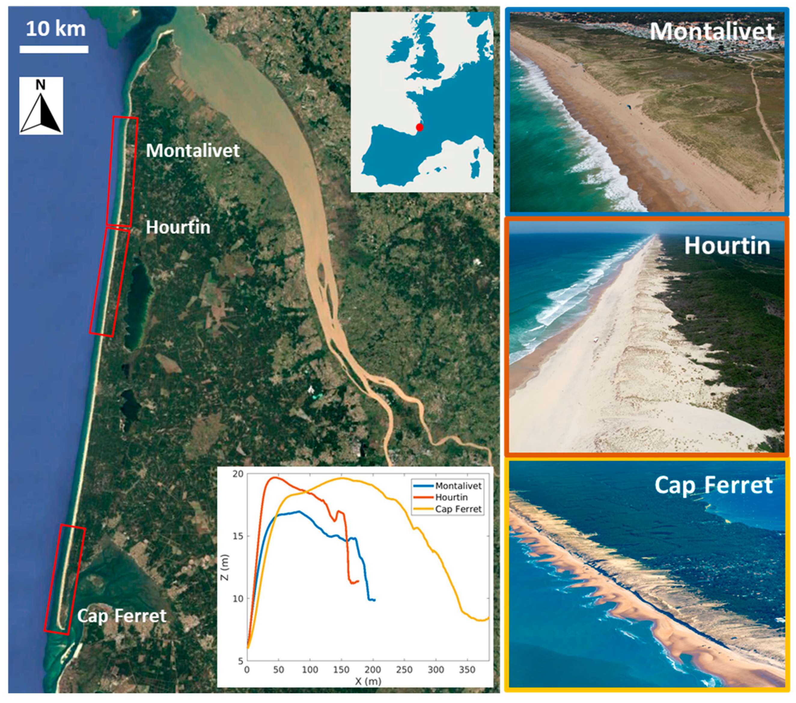
2.1. Study Sites

Three 19 km long stretches of coastal dunes located around the coastal towns of Montalivet, Hourtin, and Cap Ferret, southwest France, were selected for this study (Figure 1). This open, sandy coast is 230 km long and extends from the Gironde to the Adour estuaries. It is exposed to the North Atlantic swells with a dominant W to NW incidence [43], and the mean significant wave height ranges from 1.1 m in July to 2.4 m in January, while the mean peak wave period ranges from 8.5 s in July and 13 s in January [44]. The tidal regime is semi-diurnal and meso- to macrotidal, with a mean spring tidal range of 3.7 m. Observations along the Aquitanian coast show that the wind is mostly west and northwest-oriented and that wind speed generally ranges from 0 to 15 m/s [13]. The strongest wind events (>15 m/s) mostly occur during winter periods (from October to April). This coast is also characterized by a net southerly longshore drift of the order of 100–650 × 103 m3/year [45], and consists of intermediate and double barred beaches, with an inner intertidal bar that commonly has a transverse bar and rip channel morphology (Figure 1). The outer subtidal bar is generally well developed and often exhibits crescentic patterns with a relatively regular spacing of approximately 600–800 m [46]. All beaches are backed by a large coastal dune field [47], of which the size and shape is inherited by both natural processes and more than one century of human interventions [48]. The stretch of dunes at Montalivet, Hourtin, and Cap Ferret are on average 200, 180, and 350 m wide, respectively, and their heights vary from 10 to 25 m. Large topographic changes were observed along these dunes over the last 15 years caused by both wave impact and aeolian transport [7,44]. Dunes retreated by tens of meters during the 2013/14 storm events and, in some areas, migrated landward by another tens of meters over the subsequent 10 years [7,44]. Dune vegetation is dominated by marram grass [49], whose cover varies from one study site to another. The dunes are backed by large forests mainly comprised of maritime pines (Figure 1). Although this coastline is relatively linear and exposed to similar wave conditions, long-term shoreline changes vary along the coast [50], which affect the alongshore variability of beach and dune morphology [51].

2.2. Datasets and Methods

2.2.1. Pleiades Images

The Pleiades constellation is composed of two very high-resolution optical Earth-imaging satellites named Pleiades-1A and Pleiades-1B. This system was designed under the French–Italian ORFEO Programme and both satellites were launched in December 2011 and December 2012, respectively, with CNES (French National Spatial Agency). This constellation provides the coverage of Earth’s surface with a repeat cycle of 26 days, and offers a daily revisit capability over any point on the globe. Their orbit is sun-synchronous, phased, and near-circular and their mean altitude is 695 km. Six sets of tri-stereo Pleiades panchromatic images were acquired for this study (Table 1). The tri-stereo acquisition means that the satellites acquire three images over the area of interest within the same orbital pass. The three images are captured with different viewing angles, enabling the creation of 3D models over the area of interest. These satellite images correspond to primary level products. Images are placed in the sensor rectilinear geometry with an equalized radiometry on the native dynamic range of the sensor. They are high-resolution optical images (0.70 m for panchromatic images). The daily revisit capacity of these satellites represents a strong benefit for covering the temporal variability of coastal dune changes. The swath width of the satellites is 20 km and provides the opportunity to study coastal changes over a relatively large scale in comparison to other coastal monitoring techniques (GNSS, UAV, etc.). The images used here were obtained from DINAMIS (Dispositif Institutionnel National d’Approvisionnement Mutualisé en Imagerie Satellitaire), which provides access to high- and very high-resolution satellite imagery for numerous non-commercial users in France. DINAMIS services are provided to eligible users free of charge.

2.2.2. Ames Stereo Pipeline (ASP)

The Ames Stereo Pipeline (ASP), developed by NASA, is a suite of free and open-source automated geodesy and stereogrammetry tools designed for processing images such as Pleiades satellite images [25,26]. This toolset is developed and distributed in GitHub (https://github.com/NeoGeographyToolkit/StereoPipeline, accessed on 24 April 2025). Each set of three images is processed by pairs to generate three point clouds that are then concatenated into a single point cloud used to produce a DEM. The workflow used here to generate DEMs from Pleiades images can be divided into six main steps: bundle adjustment, image alignment, correlation, blending, filtering, and triangulation. First, satellite position and orientation errors have a direct effect on the accuracy of the DEMs produced with ASP. The errors in camera position and orientation have been corrected using a process called bundle adjustment, where the properties of the cameras and the 3D locations of the objects they capture are simultaneously adjusted. This adjustment ensures that the observations in multiple images of a single ground feature are self-consistent and is carried out along with thousands of similar constraints involving many different features observed in the different images. After being adjusted, images were aligned since they are captured from different perspectives. The affine epipolar alignment method was used and allows us to pre-align the images. Then, a matching algorithm is used for the correlation step, which involves identifying pixel correspondences between the epipolar images and generating the corresponding disparity maps. The sub-pixel correlation mode was set to mode 3 here, as advised by the ASP developers, and was applied to refine the disparity maps by removing some staircasing and other artefacts. The More Global Matching (MGM) algorithm [52] was selected since it reduces the amount of high-frequency artefacts in textureless regions, such as bare sandy coastal dunes. However, this algorithm requires a longer computing time in comparison to other matching algorithms. For each pixel in one image, the algorithm matches a small block around this pixel with another similar block in the other images. The block size, also called the kernel, can be defined and was set to 7 pixels here, which is a good compromise between the performance of the algorithm and computation time. The selected image operator was the Census Transform [53], which associates a binary string to each pixel that encodes whether or not the pixel has a smaller intensity than each of its neighbors. This operator performs well for environments with uncontrolled lighting, such as coastal areas. Following this correlation step, the borders of adjacent disparity map tiles are blended, and the same map is filtered with potential holes that are filled by an in-painting algorithm. Finally, a 3D point cloud is generated by performing a triangulation of the disparity map that is used to build a DEM on a 1 × 1 m grid at the same resolution as the LiDAR DEMs (Section 2.2.4)

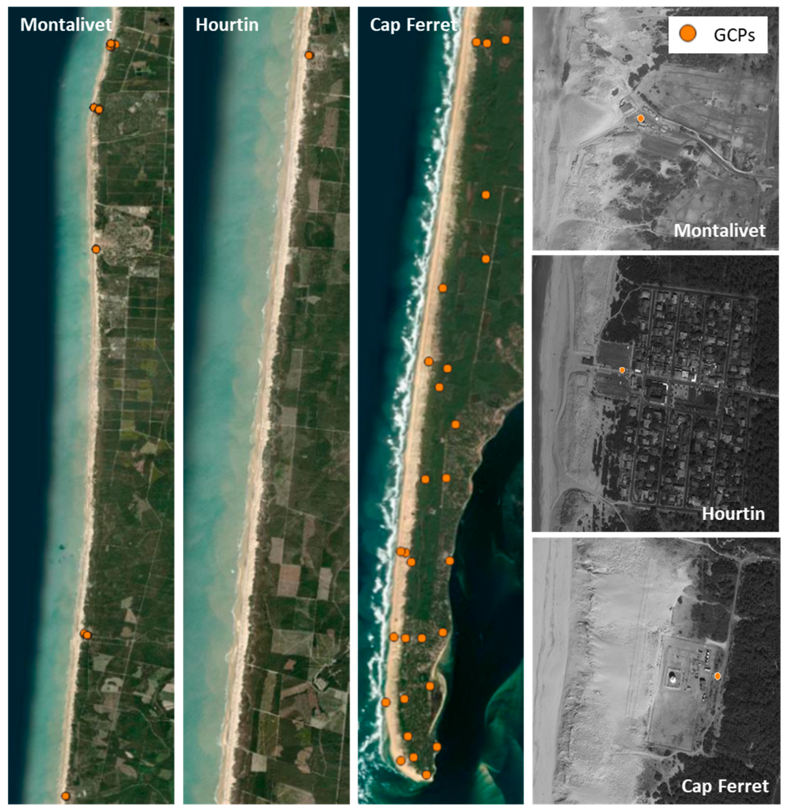
2.2.3. Ground Control Points (GCPs) for Pleiades DEMs Altimetry Correction

RTK-GNSS data points collected at the three study sites (Figure 2) were not used during the bundle adjustment process using ASP but were subsequently employed as GCPs to correct the vertical offsets of the Pleiades DEMs, and to convert them from an ellipsoidal datum (WGS84) to the local vertical coordinate system (NGF—IGN69). Since these data points were collected after the Pleiades images acquisition, they were surveyed over solid ground (roads, parking lot, bunkers, etc.), ensuring that the elevation of these data points has not changed between both data acquisitions, separated by several years. The number of data points (Table 2) and their spatial distribution (Figure 2), strongly vary from one site to another because they rely on the availability of infrastructures present at each study site. Urbanized areas such as Montalivet and Cap Ferret offer the opportunity to collect many GCPs (63 and 24, respectively), while only a few GCPs were acquired at Hourtin (5).
An altimetry correction factor, Zcorr, was calculated using a simulated annealing non-linear optimization algorithm [54], which has shown good results in other recent coastal research applications [55,56,57]. Simulated annealing is based on a non-linear probabilistic method, where a global minimum of a cost function, defined here as the vertical difference between RTK-GNSS and Pleiades Z values for each GCP, is considered as the optimum solution. This solution corresponds here to the altimetry correction factor, which is calculated for each Pleiades DEM and at each study site. Although the exact same GCPs are used at each study site, the correction factors, Zcorr, can vary from one set of images to another, with a difference up to 8.5 m (Table 2). Such a method does not necessarily guarantee the best accuracy of the Pleiades DEMs in comparison to other post-processing methods based on co-registration and polynomial transformation using ortho-images [41], or methods using beach profiles to determine a vertical offset between Pleiades and in situ data [42]. However, this method was used here because it is easily replicable since it only requires relatively basic equipment (GNSS), and because the same GCPs can be collected either before or after the Pleaides images and can be used for any set of Pleiades images. Furthermore, this processing does not require the user to perform any manual tasks.

2.2.4. Large Airborne LiDAR Data for Pleiades DEMs Validation

DEMs derived from airborne LiDAR data collected at the three study sites by the Observatoire de la Côte de Nouvelle-Aquitaine (OCNA) can be downloaded here (https://portail.pigma.org/, accessed on 24 April 2025) and were used to assess the accuracy of Pleiades-derived DEMs. Topographic values, Z, extracted from both LiDAR and Pleiades DEMs, are interpolated on the same 1 × 1 m grid and compared using the Pearson coefficient of correlation (R), root mean squared error (RMSE), and bias (B). The differences between Pleiades and LiDAR DEMs were also plotted and are presented within the next section to observe the spatial distribution of the difference in Z values, dZ, over each of the three entire stretches of coastal dunes. Although Pleiades images also cover beach areas, these were excluded from the analysis due to their strong seasonal variability that is much larger than dunes [44,51]. This exclusion was necessary to prevent natural topographic changes from skewing the assessment of the Pleiades DEMs vertical errors. The seaward limit of the dune areas corresponds to the dune foot (Z = 6 m), while the landward limit corresponds to the forest line located at the back of the dune at the three study sites. Beach and pine forest areas were therefore masked from the Pleiades and LiDAR DEMs.

3. Results

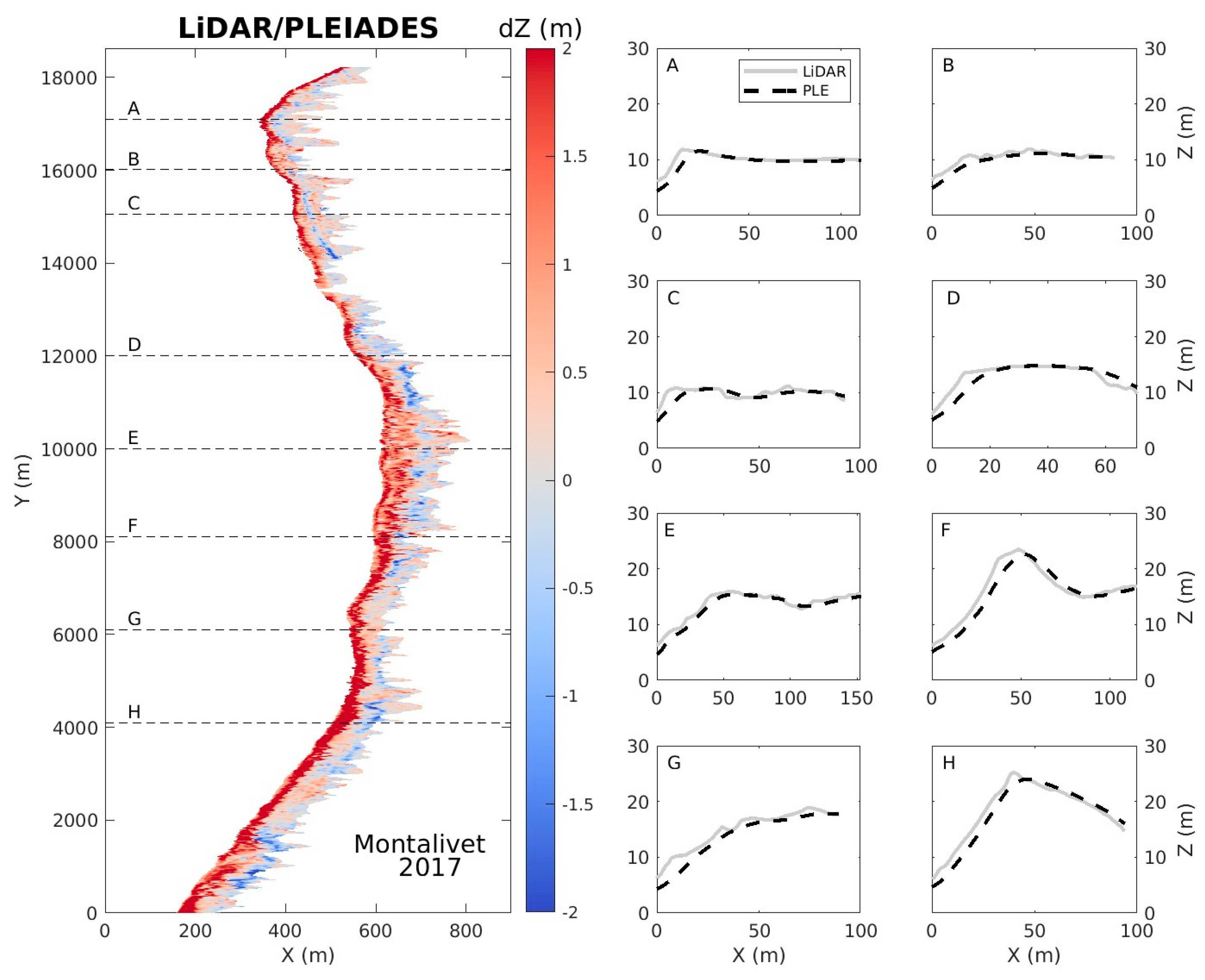
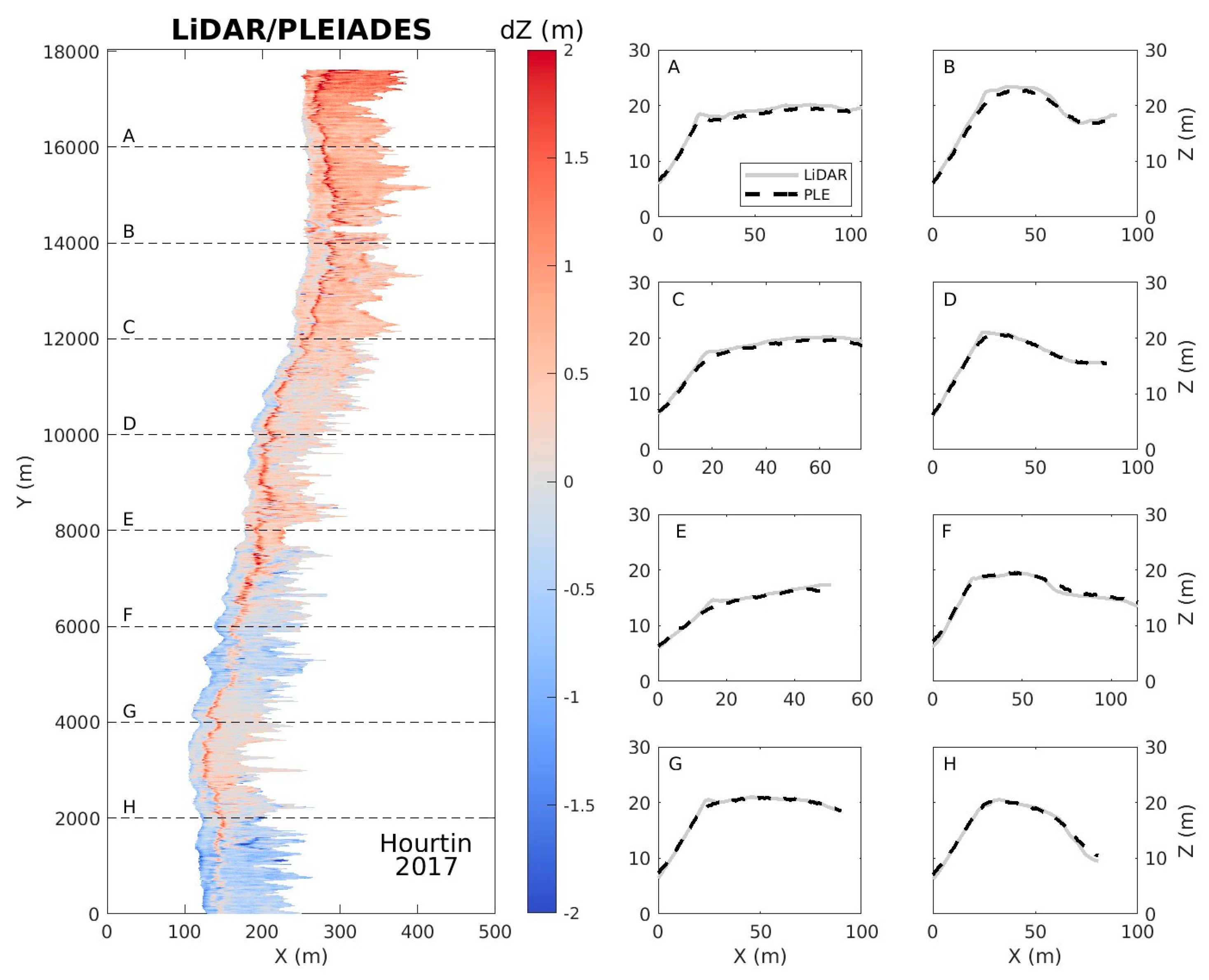
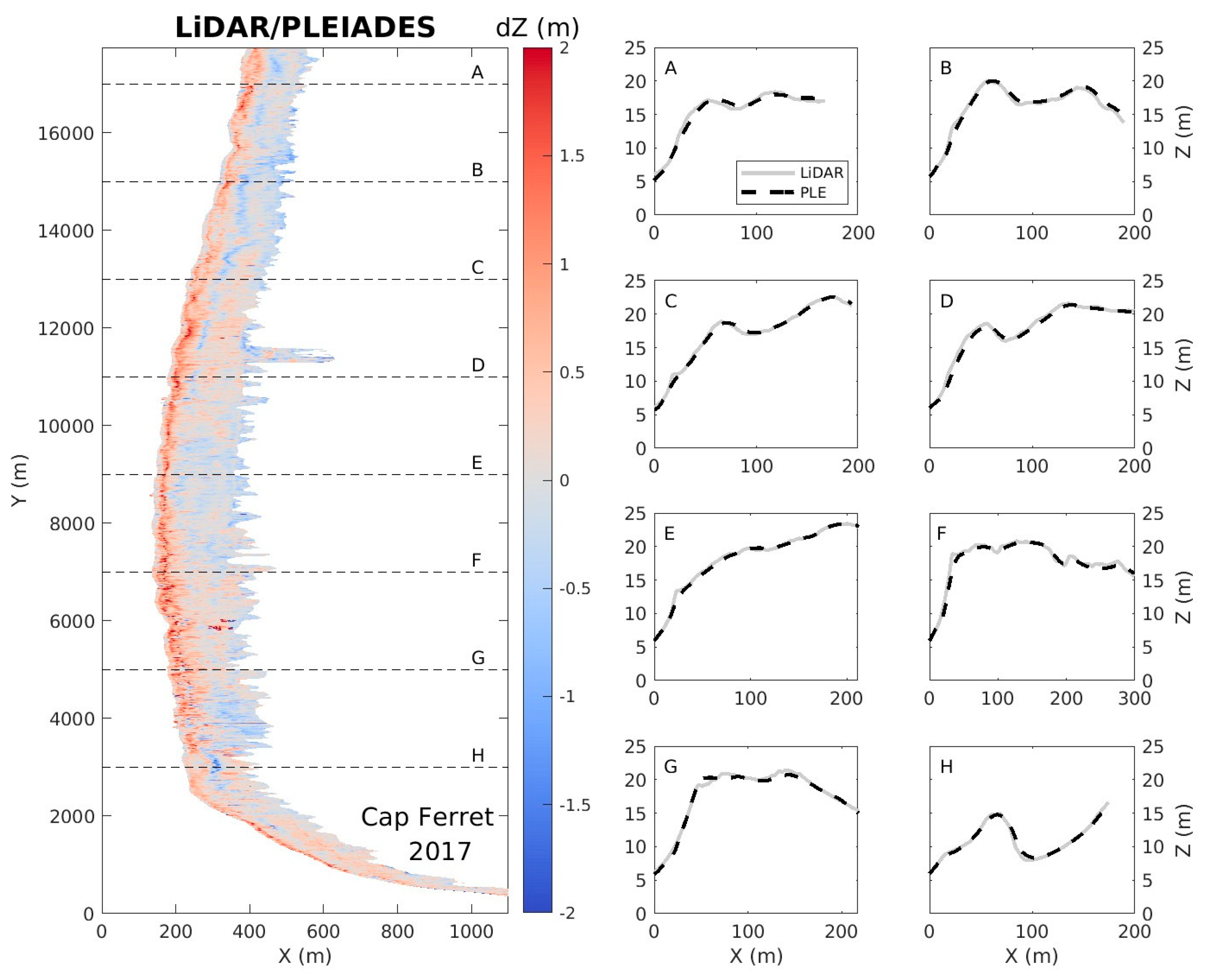
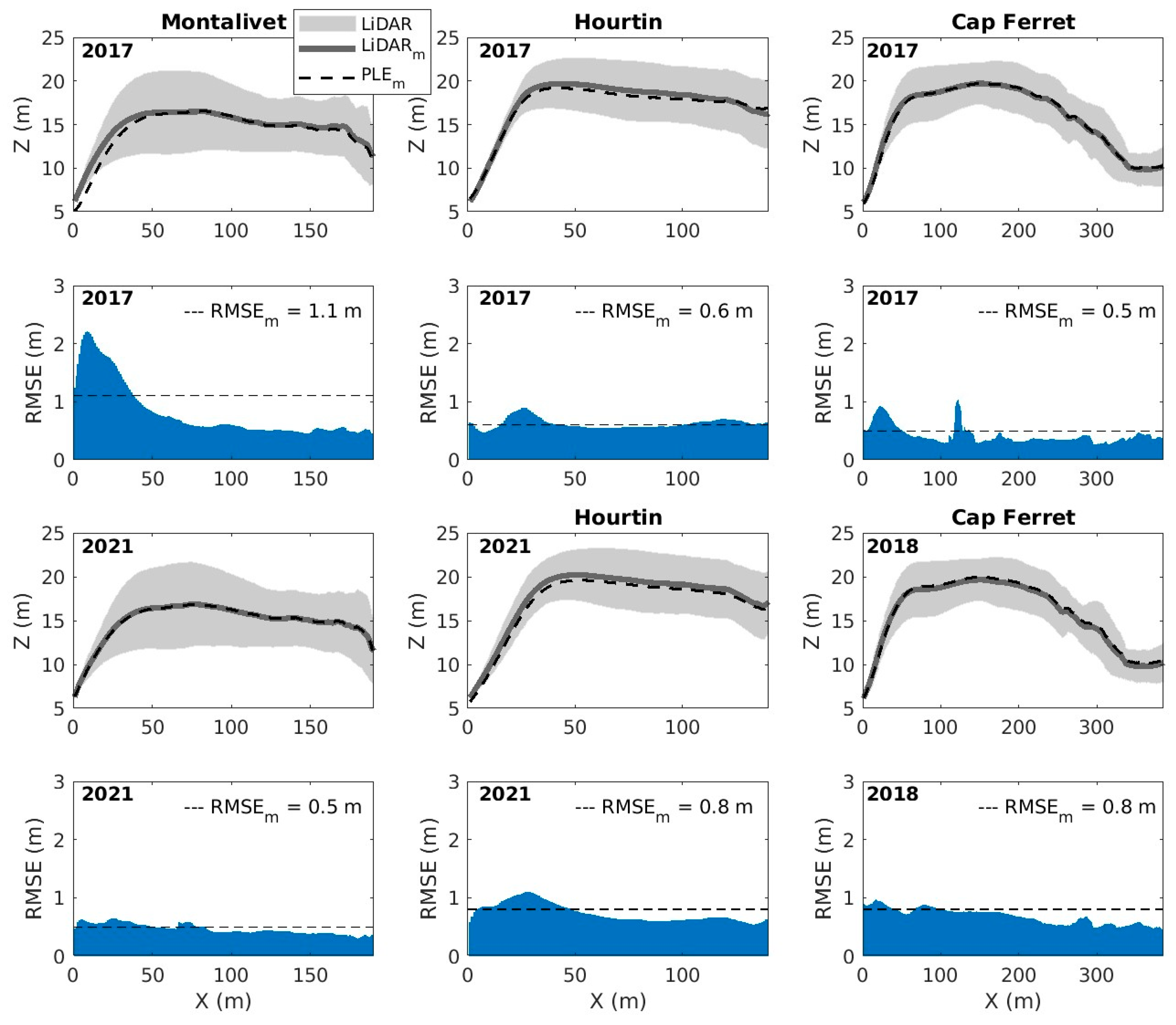
3.1. Comparison Between Pleiades and LiDAR DEMs

Three examples of the six DEMs derived from Pleiades images using ASP are presented in Figure 3. These DEMs highlight the alongshore variability in dune topography at each study site with elevations, Z, ranging from 5 to 30 m.
The Pleiades and LiDAR DEMs were compared to assess the performance of the ASP to generate 3D elevation models from tri-stereo Pleiades images. As stated in the previous section, the Pearson correlation coefficient (R), root mean square error (RMSE), and bias (B) were used to compare each 1 m-cell of both DEM dune areas and are presented in Table 3. Correlation coefficients are all above 0.98, averaged RMSE values vary from 0.51 to 1.12 m, and averaged B values range from −0.59 to 0.15 m. These values are not site specific, since they vary between the three study sites and from one DEM to another corresponding to the same study site. The topographic variations are reproduced well (high R values), although local errors can be relatively high (RMSE values > 1 m), and except for the set of images collected at Cap Ferret in 2018, altimetry is always underestimated on the Pleaides derived DEMs in comparison to the LiDAR ones.
Three examples of the difference between the Pleiades and LiDAR DEMs are presented in Figure 4 (Montalivet 2017), Figure 5 (Hourtin 2017), and Figure 6 (Cap Ferret 2017), where the spatial distribution of the elevation differences, dZ, can be observed. Although the amplitude of the dZ values vary from one site to another, the largest differences can be observed along the dune stoss slope (i.e., seaward dune face) at the three study sites, whereas they are smaller at the top and back sides of the dunes. The Pleiades-derived DEM from the set of images collected at Montalivet in 2017 corresponds to the largest averaged RMSE value (1.12 m) among all the sets of images studied here (Table 3). The comparison of Pleiades and LiDAR DEMs, and corresponding examples of cross-shore dune profiles at Montalivet in 2017 (Figure 4), shows that dune topography along the dune stoss slope is more than 2 m lower in the Pleiades DEM in comparison to the LiDAR one (profiles from A to H). While Z values are underestimated at the dune stoss slope on the Pleiades DEM, they are overestimated along the back of dunes with relatively steep slopes (profiles D, F, and H). However, when dune profiles are characterized by a plateau that ranges from 50 to 100 m (profiles A, B, C, D, and E), differences between Pleiades and LiDAR DEMs are small along these plateaus (<0.5 m). At Hourtin in 2017, the averaged RMSE value is much smaller (0.63 m). While the dune stoss slope and the back of the dune are very well correlated, a narrow area around the dune crest highlighted by a thin red line can be observed along the differences between the Pleiades and LiDAR DEMs (Figure 5). This area is characterized by a pronounced change in slope along the dune profile (profiles A, B, C, D, E, and G). The DEM derived from the set of images acquired at Cap Ferret in 2017 corresponds to the DEM with the lowest RMSE value (0.51 m) of all sets of images used in this study. Like Hourtin 2017, the performance of the ASP is lower where the dune profile shows strong changes in slope (Figure 6). For instance, changes in slope are observed at the dune crest (profiles E, F, and G) or where there is a small foredune along the dune stoss slope (profiles B, C, and D), while the rest of the dune profile is reproduced well on the Pleiades DEM.
The alongshore-averaged cross-shore dune profiles and the longshore-averaged RMSE values along the cross-shore axis are presented in Figure 7 to give an overall view of the spatial distribution of the errors at all study sites, and for all the sets of images used to generate Pleiades DEMs. Results show that the amplitude of the RMSE spatial distribution varies among study sites and from one set of Pleiades images to another. The distribution of the errors across the dune profile (along the X axis) can either be almost even (Montalivet 2021), unimodal (Montalivet 2017, Hourtin 2017, and Hourtin 2021) or multimodal (Cap Ferret 2017, and Cap Ferret 2021). As observed in the differences between the Pleiades and LiDAR DEMs presented in the previous figures, the largest errors at the three study sites can be mostly found within the first 50 m that correspond to the dune stoss slope and crest, which are the steepest parts of the dunes and can be explained with different reasons. Errors in altimetry can either be due to planimetric errors during satellite image acquisition or the 3D reconstruction process and are amplified over steep terrain. They can also be due to the presence of large shadow areas on satellite images that appear over steep terrain in the function of the angle orientation of the topography in relation to the sun light and the satellite viewing angle. These shadow areas have low reflectance and texture in comparison to the other image pixels, causing errors in altimetry. For example, every peak of RMSE at the Cap Ferret study site corresponds to an abrupt change in slope across the dune profile (Figure 7). Furthermore, aeolian sediment transport is generally active at the dune stoss slope because of the compression of the flow field over steep slope that increases shear stress [58]. Possible errors due to the time difference between the acquisition of Pleiades images and the airborne LiDAR survey are thus expected to be larger at the dune stoss slope and crest.

3.2. Satellite-Derived Coastal Dune Morphological Change

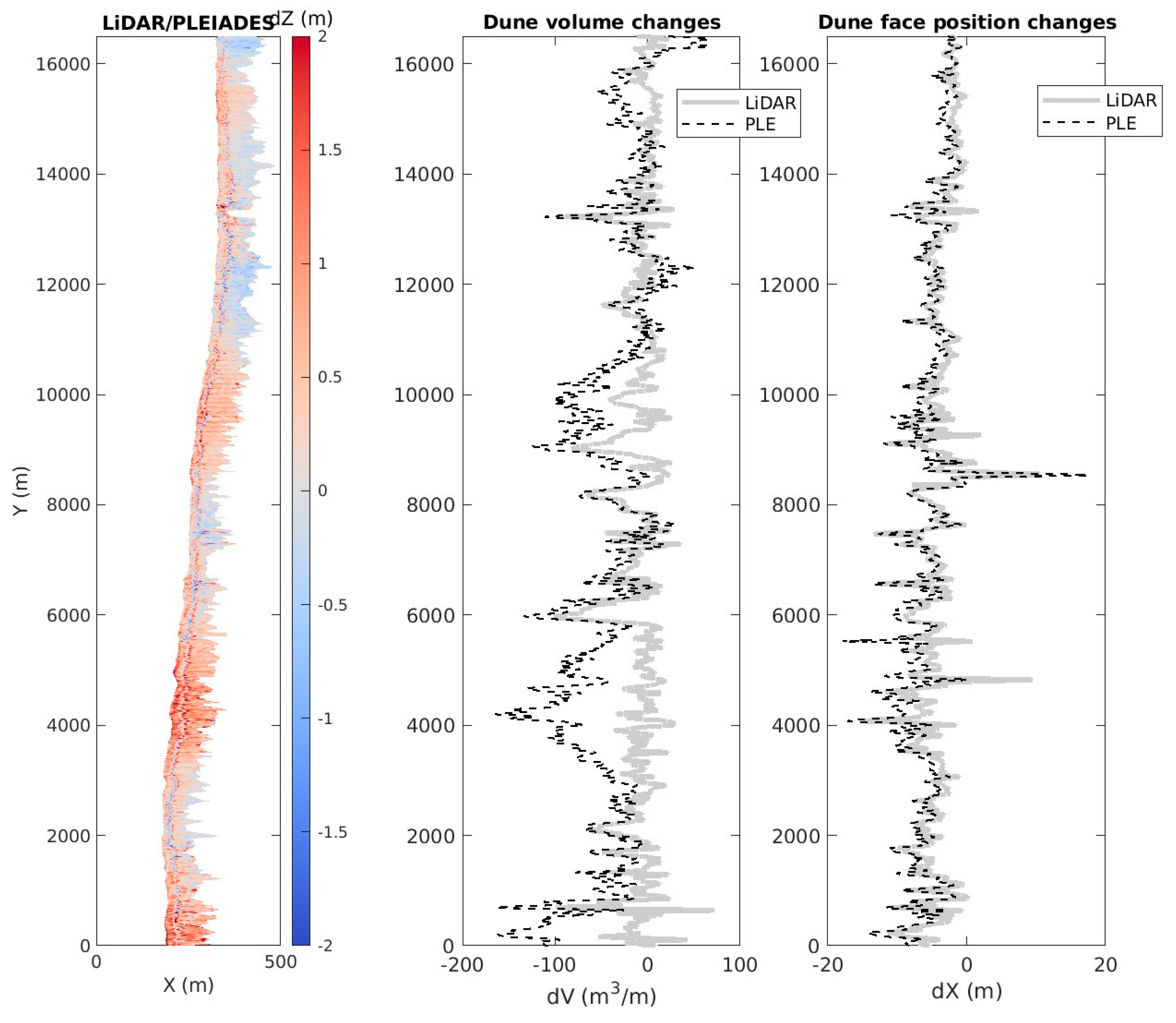
3.2.1. Large-Scale Patterns of Coastal Dune Changes

Given the large coastal dune morphological changes typically observed in southwest France [7,13,51], and the fair performance of the ASP to produce DEMs (Section 3.2), we explored the potential of the Pleiades satellite constellation to monitor temporal coastal dune changes from the two sets of images acquired at Hourtin in 2017 and 2021. Such analysis was not carried out at Montalivet because of the large errors of the 2017 Pleiades DEM (RMSE = 1.12 m, Table 3). Although the Pleiades-derived DEMs at Cap Ferret in 2017 and 2018 show smaller errors (RMSE = 0.51 and 0.78 m), temporal dune changes at this site is not explored here since the magnitude of the topographic changes over that year is too small in comparison to the DEM generation errors. The averaged absolute value of elevation change (i.e., gross change) between 2017 and 2018 at Cap Ferret is 0.13 m, which is almost 5 times lower than the errors between the 2017 Pleiades and LiDAR DEMs. In comparison, the averaged absolute value of elevation change at Hourtin between 2017 and 2021 is 1.02 m. When comparing the differences between DEMs obtained through Pleiades and LiDAR at Hourtin, erosion/accretion patterns are similar (Figure 8). The differences between the 2017 and 2021 LiDAR DEMs (dZ = Z2021Z2017) show alongshore uniform patterns of erosion at the dune stoss slope all along the study site, which are reproduced well on the Pleiades DEMs. While the vertical accretion at the upper part of the dune observed at the northern part of the site (from Y = 11,000 to Y = 14,000 m) is captured well on the Pleiades DEMs (dZ < 0.5 m), accretion with similar amplitudes is underestimated (dZ > 2 m) at the southern part of the site (from Y = 0 to Y = 500 m and from Y = 3500 to Y = 5500 m). Three examples of cross-shore dune profiles with contrasting morphologies are also presented in Figure 8, showing that dune retreat with different amplitudes observed on the LiDAR DEMs are reproduced well on the Pleiades DEMs despite small topographic differences, especially at the dune crest.
Dune volume changes (dV in m3/m) or dune foot/stoss slope position changes (dX in m) are commonly quantified in coastal studies to describe dune changes. Results show that Pleiades-derived DEMs can be used to approximate the total volume of sand of a dune system, Vtot, since all volumes are within the same order of magnitude despite the vertical errors of the Pleiades DEMs (Vtot = 2.78 × 10⁷ and 2.77 × 10⁷ m3 in 2017 and 2021 based on the LiDAR DEMs, and Vtot = 2.74 × 10⁷ and 2.67 × 10⁷ m3 based on the Pleiades DEMs). However, these differences in Vtot are too large to have a good estimate of the temporal total volume changes, dVtot, even though both numbers indicate dune erosion at Hourtin between 2017 and 2021 (dVtot = −1.51 × 10⁵ m3 based on the LiDAR DEMs, and dVtot = −6.56 × 10⁵ m3 based on the Pleiades DEMs). The alongshore differences in dV can be observed in Figure 9, and similarly to the differences between DEMs presented in Figure 8, the temporal dune volume changes are reproduced relatively well by the Pleiades DEMs at the northern part of the study site (from Y = 6000 to 16,000 m). The erosion is slightly overestimated between about Y = 9000 and 11,000 m and between Y = 15,000 and 16,000 m. Erosion is overestimated at the southern part (from Y = 0 to 6000 m). However, the temporal dune changes quantified on the Pleiades DEMs can be representative of the observed ones when considering dune stoss slope position as a parameter to monitor such change (Figure 9). Here, the proxy Z = 13 m was selected to ensure the alongshore continuity of the variations and to capture the dune stoss slope retreat measured at Hourtin. However, similar alongshore variations were obtained when testing other elevation proxies ranging from 10 to 15 m. Results for Z = 13 m show that the alongshore variations of the temporal dune stoss slope position changes, dX, extracted from the LiDAR and Pleiades DEMs overlap (Figure 9). When dune stoss slope position changes are averaged over the entire study site, dXavg, the dune stoss slope retreat is overestimated by 1.3 m on the Pleiades DEMs (dXavg = −4.33 m based on the LiDAR DEMs, and −5.57 m based on the Pleiades DEMs). The alongshore variability in both dune volume and dune stoss slope position changes that, respectively, range from −169 to +103 m3/m and from −18 to +11 m, can be explained by the alongshore diversity in dune morphology but also by the presence of dune blowouts that are further discussed in the next section.

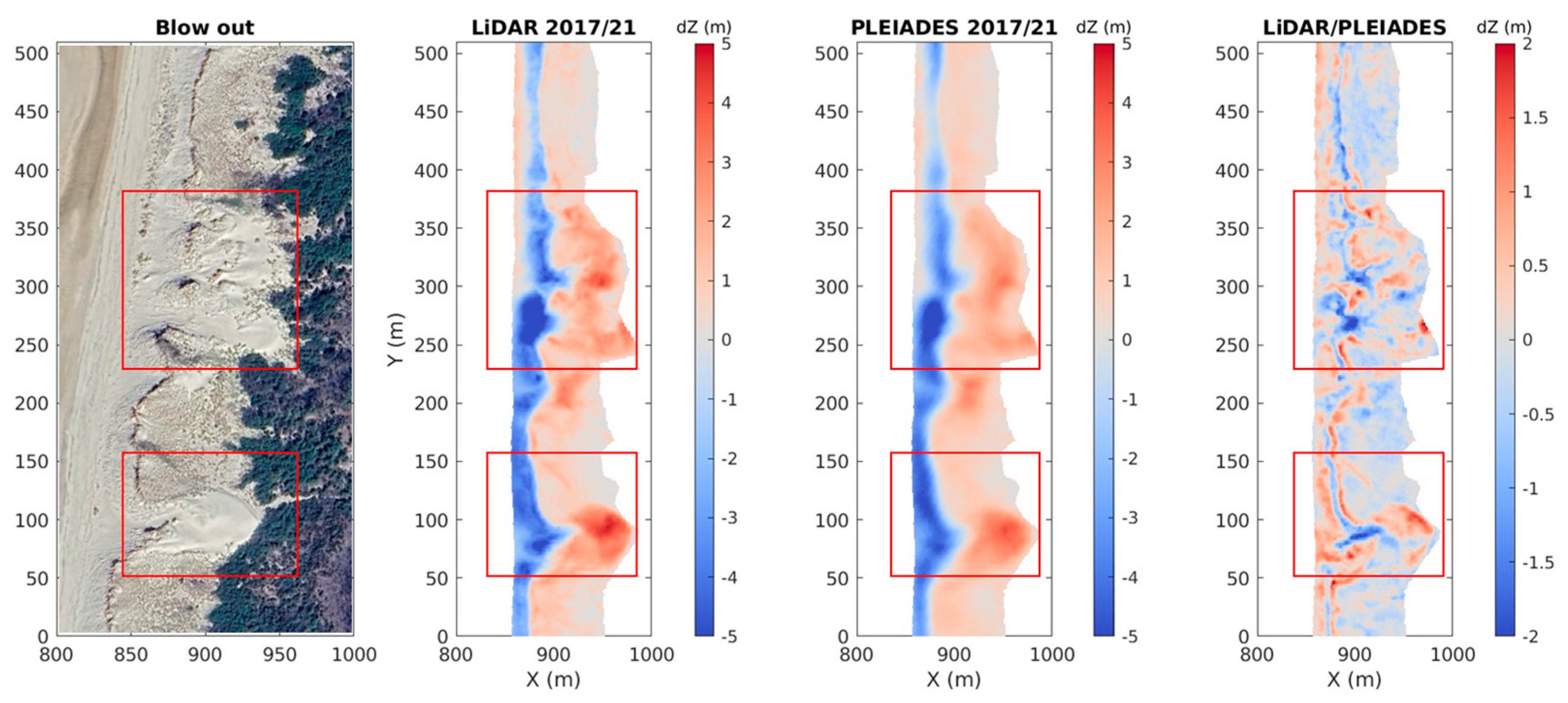
3.2.2. Coastal Dune Blowout Dynamics

In the previous section, Pleiades DEMs were shown to be useful in monitoring temporal coastal dune changes over tens of kilometers. These changes were characterized by strong alongshore variations due to the non-uniform topography of the dunes over tens or hundreds of meters. Blowouts are sandy depressions caused by aeolian transport and represent a challenge for coastal managers since blowouts are highly dynamic during strong windy events. Along the Aquitaine coast, blowouts can range from a few meters to kilometers, and can rapidly migrate landwards into the pine forests located behind the dunes [11,47]. Three blowouts located at the Hourtin study site were taken as examples and are shown in Figure 10. The blowouts, which are highlighted by red squares, correspond to the bare sand areas that are concave on the seaside (west) and convex on the forest side (east), in line with the main wind direction that is from west to east. The temporal differences between the 2017 and 2021 LiDAR DEMs show strong erosion at the dune stoss slope and strong accretion at the back of the blowouts (Figure 10). Part of the erosion over the dune stoss slope was possibly due to marine forcing reaching the dune foot area, while another part of this eroded sand was transported by wind through the blowouts and accumulated to the back of the dune. These processes caused a partial landward migration of the dune. The temporal differences between the 2017 and 2021 Pleiades DEMs shows the same patterns of erosion and accretion (Figure 10) demonstrating the ability of satellite remote sensing to capture the formation and subsequent evolution of blowouts. As mentioned in the previous section, the largest errors are observed along the dune crest (from Y = 100 to 200 m, and from Y = 400 to 450 m), but they are also located at the center area of the blowouts (Y = 85, 270, and 305 m) and over its flanks, which usually are one of the steepest parts of the dune.

4. Discussion

4.1. Performance and Sources of Errors

This study showed that tri-stereo Pleiades panchromatic images can be successfully used to provide DEMs with a relatively good accuracy. The averaged vertical root mean square errors of the six DEMs derived from six sets of Pleiades images, using the Ames Stereo Pipeline [25,26], range from 0.51 to 1.12 m, with respect to airborne LiDAR data. The range of vertical errors presented here are within the range of two other coastal studies using the same methodology [41,42]. The overall RMSE value was 0.35 m at one study site located in SW France for one pair of Pleiades images [41], while the overall RMSE values were, respectively, 1.31 m and 1.15 m for two sets of Pleiades images acquired over one study site located along the west coast of Senegal [42]. It should be noted that a better accuracy would be expected here if the time difference between the acquisition of Pleiades images and the airborne LiDAR surveys was smaller. Indeed, except one set of Pleiades images captured in August 2018 at Cap Ferret, the other sets were captured in April (Table 1), while airborne LiDAR surveys were all carried out in October. Although the months between April and October correspond to summer periods along the SW coast of France, which are characterized by relatively low energy wave and wind conditions [47] and thus, small topographic changes [19], the topography of coastal dunes can change over these six months and represent a source of error when comparing Pleiades and LiDAR DEMs. However, results showed here that the smallest time difference between both data acquisitions (Cap Ferret 2018, 2 months) does not correspond to the smallest RMSE value (0.78 m), suggesting that other sources of error are more significant.
In addition to the errors associated with the 3D reconstruction of the Pleiades-derived DEMs using ASP and the time difference between the Pleiades images and LiDAR data acquisition, other sources of errors can be identified and are related to either the inherent characteristics of the Pleiades images acquisition, or to the method used to process them.
The comparison of RMSE values between the six DEMs show that accuracy is mostly image-specific rather than site-specific. This lack of consistency between satellite images can be explained by the varying environmental conditions during image acquisition, which introduce environmental noise and alter the radiometric quality of the reflectance values recorded by the satellite sensors [59]. As an example, the altimetry correction factor, Zcorr, applied in this study, varied by ten meters between the different sets of images (from −44 to −55 m, Table 2). Collecting ground truth data is, therefore, required before making the comparison of DEMs derived from Pleiades images acquired at different times. The use of these ground truth data for the post-processing of Pleiades-derived DEMs can also have an impact on the DEM accuracy. They can be collected over beach and dune areas to calculate a vertical offset with Pleiades elevations [41,42] or used for planimetric corrections [41]. In this study, GNSS data points (GCPs) were only used to calculate an image-specific vertical correction factor, Zcorr, to account for the vertical offset between both Pleiades and LiDAR DEMs, and is applied to the entire Pleiades DEM so they can be compared. These data points were collected over solid ground (roads, parking lots, bunkers, etc.), after the Pleiades acquisition time and outside of the beach/dune areas. Such data collection protocol and method can be easily replicable in other coastal areas and gives the opportunity to make use of any archived Pleiades images. Results showed that the number and spatial distribution of the GCPs do not necessarily impact the accuracy of the DEMs. Although only five GCPs could be collected within a small area at Hourtin because there were only a few areas with solid ground at this study site, RMSE values were relatively low (0.63 and 0.80 m) in comparison to Montalivet (1.12 m), where 63 GCPs were collected. Furthermore, tests were made where the number of GCPs are reduced from 63 to 40, 20, and 10 when calculating Zcorr at Montalivet. This reduction did not significantly impact the accuracy of the DEMs.
Another source of error that is not explored in this study is the impact of the presence of vegetation over dunes. Both Pleiades images and airborne LiDAR are sensitive to vegetation, but filters were applied to compensate for this and represent bare ground on the LiDAR DEMs by the LiDAR data providers (OCNA). No filter has been applied here on the Pleiades-derived DEMs, and they should thus be considered as DSMs, but filters should be applied in future analysis for better accuracy when comparing to LiDAR data. Dune vegetation cover and densities show strong spatial and temporal variability; image-specific filters should therefore be produced to account for this variability. However, results showed that the largest errors on the Pleiades DEMs were located on the dune stoss slope where vegetation is usually not present because of active sediment transport [49]. Indeed, in agreement with observations made in [41], the results showed that the largest errors in altimetry on the Pleiades images are located on the dune stoss slope and dune crest, which correspond to the steepest part of the dunes, and where shadow areas are likely to be observed. These shadow areas have low reflectance and texture, causing errors in the elevation calculation. The steepness of the Aquitanian dunes stoss slopes can cause the appearance of shadow areas, but can also cause errors in altimetry by increasing the chance of planimetric errors during satellite image acquisition or the 3D reconstruction process. The satellite viewing angles of the sets of images analyzed in this study vary from one image to another (Table 1) but do not necessarily explain the accuracy of the 3D reconstruction. Pleiades-derived DEMs from two sets of images collected at the same study site (Montalivet) with similar angles (7.7°/0.2°/−7.5° and 7.5°/−0.02°/−7.5°) have different averaged RMSE (1.12 and 0.53 m, respectively). This demonstrates that both minimizing shadow areas by defining optimized viewing angles and improvements in the 3D reconstruction process (e.g., bundle adjustment, matching algorithm, etc.) are required to reduce the errors in altimetry on the Pleiades-derived DEMs.
Even though many potential sources of errors have been identified above, this study showed that tri-stereo Pleiades panchromatic images can be successfully used to monitor multi-annual coastal dune morphological changes at spatial scales ranging from meters to tens of kilometers. This range of error remains relatively high in comparison to GNSS and UAV surveys that provide topographic datasets with a vertical accuracy of a couple of centimeters [14,17]. Airborne LiDAR surveys usually provide data with a vertical accuracy between 10 and 20 cm [13,60,61], and their spatial coverage can be similar to the Pleiades images (tens of kilometers). Although the vertical errors of Pleiades-derived DEMs are currently too high to monitor dune evolution on seasonal or annual scales when no energetic waves or winds are recorded [7,13], this study shows that they can be used to monitor dune topographic changes along the Aquitanian coast on a multi-annual scale or following storm events. Furthermore, it was shown that the choice of the proxies to study coastal dune dynamics can be adapted to the limits of Pleiades-derived topography. The average dune stoss slope retreat of 4.3 m at Hourtin between 2017 and 2021 was effectively captured by the Pleiades images with a reasonable error (+1.3 m or 30%). In coastal areas where there is no existing implemented coastal monitoring, the use of Pleiades images can be considered as a cost-effective alternative for mapping coastal dune topography while remaining aware of the associated uncertainties when developing coastal management strategies. Where coastal monitoring has been implemented (e.g., GNSS, UAV, and LiDAR surveys), the use of Pleiades images can be integrated in a hybrid monitoring framework. During extreme events, the operational requirements and financial cost of beach and dunes surveys limit their immediacy while the agility and daily revisit capacity of Pleiades satellites represent strong benefits for urgent decision-making. Along the Aquitanian coast, where dune heights exceed 20 m and can retreat by several meters during a single storm event [7,44], DEMs with one-meter horizontal and vertical errors remain suitable with regard to risk thresholds definition for hazard forecasting (e.g., erosion limits, overtopping risks, etc.).

4.2. Future Perspectives

The current performance of the 3D reconstruction of digital elevation models derived from Pleiades images highlights their value as tools to monitor morphological changes over large stretches of coastal areas. However, it is essential to remain aware of the associated uncertainties to ensure accurate interpretation and avoid misrepresentation of the data. Furthermore, many ongoing or future improvements are expected to improve the vertical accuracy of these elevation models. Besides the regular improvement of pixel matching algorithms, different pipelines which are based on different stereo matching algorithms, such as MicMac [27] and CARS [28], can show better performance and are more adapted to specific topographic features corresponding to a certain type of environment. However, Pleiades-derived DEMs produced with CARS over a beach area showed larger vertical errors than the same ones produced with ASP [62].
Another significant improvement in the production of DEMs from Pleiades images could originate from the new Pleiades Neo constellation, launched in 2021 and 2022, which provide panchromatic images with a spatial resolution of 0.30 m at nadir [63]. This improved resolution can potentially reduce vertical errors observed in this study and others by more accurately capturing the sharp changes of slope at the dune stoss slope and crest. The daily revisit capacity of the Pleiades satellites can also be used to determine the most adequate viewing angles between the three images that minimize shadow areas by ordering several images, within a short period of time, to ensure similar sun exposure conditions (altitude and azimuth) and the absence of morphological changes occurring at the dune stoss slope.
Another application of the use of Pleiades images that is not explored here but will be in the future is vegetation mapping [39]. In addition to increasing the accuracy of Pleiades-derived DEMs by filtering the vegetation as mentioned above, Pleiades images can be used to produce large scale maps of coastal dune vegetation cover. Temporal and spatial variations in vegetation type, density, and abundance play a key role in coastal dune morphological change [64]. The high resolution of Pleiades Neo images can potentially lead to the classification and identification of plant species for a better understanding of vegetation dynamics [48].

5. Conclusions

The vertical accuracy of digital elevation models (DEMs) derived from tri-stereo panchromatic and high-resolution Pleiades images was shown to be suitable to monitor multi-annual coastal dune morphological changes. It was demonstrated that the Pleiades-derived DEMs could reproduce well the overall dune topography along with erosion and accretion patterns over large spatial scales (>15 km) and allow us to quantify dune retreat with small errors. These images could thus be used to quantify erosion at a kilometric scale during energetic events (e.g., storms), and be integrated into early warning systems to assess the risks of overwash and flooding a few days prior to the storm event.
Although the vertical accuracy of Pleiades-derived DEMs (0.5–1 m) remains 5 to 10 times lower than that of airborne LiDAR and UAV data (0.1–0.15 m), Pleiades images offer a cost-effective alternative for mapping coastal dune topography on a global scale using open-source stereophotogrammetry tools (e.g., Ames Stereo Pipeline). Furthermore, only a limited number of field-collected elevation points are required to perform a simple vertical correction on the generated Pleiades DEMs.
Shadow areas due to the steepness of the dune stoss slope and the viewing angle of the satellite, with regards to the sun, along with planimetric errors, remain the major causes of errors still limiting accurate enough volumetric changes assessment. The regular improvement of stereo matching algorithms, such as the agility and daily revisit time of Pleiades satellite, provides the opportunity to statistically define a viewing angle that minimizes shadow areas. Furthermore, the launch of new satellites constellations, such as Pleiades Neo, which provide panchromatic images with a spatial resolution of 0.3 m, highlights the growing potential of Pleiades data. These developments advocate for its broader application in coastal research, including topography and bathymetry reconstruction, vegetation mapping, and other related studies, contributing significantly to our understanding and management of coastal systems worldwide.

Author Contributions

Conceptualization, O.B. and B.C.; methodology, O.B.; formal analysis, O.B.; writing—original draft preparation, O.B.; writing—review and editing, O.B., B.C., V.M., B.L., A.N.L., and N.R.; supervision, B.C. All authors have read and agreed to the published version of the manuscript.

Funding

This research was funded by the European Commission with the Horizon 2020 Framework Programme (H2020) and Marie Sklodowska-Curie Actions (H2020-MSCA-IF-891807).

Data Availability Statement

Airborne LiDAR campaigns were commissioned by the Observatoire de la Côte de Nouvelle-Aquitaine (OCNA) and can be downloaded here (https://portail.pigma.org/, accessed on 24 April 2025). Pleiades images were distributed by DINAMIS—for Dispositif Institutionnel National d’Approvisionnement Mutualisé en Imagerie—funded by CNES, CNRS, IGN, IRD, INRAE and CIRAD.

Acknowledgments

The authors would like to thank the Observatoire de la Côte de Nouvelle-Aquitaine (OCNA) and DINAMIS for providing airborne LiDAR data and Pleiades images, respectively. They would also like to thank the reviewers for their comments that helped to improve the manuscript.

Conflicts of Interest

The authors declare no conflicts of interest.

Abbreviations

The following abbreviations are used in this manuscript:
ASPAmes Stereo Pipeline
CNESCentre National d’Etudes Spatiales
DEMDigital Elevation Model
DINAMISDispositif Institutionnel National d’Approvisionnement Mutualisé en Imagerie
GCPGround Control Point
GNSSGlobal Navigation Satellite System
LiDARLight Detection And Ranging
NWNorthwest
RMSERoot Mean Square Errors
SWSouthwest
UAVUnmanned Aerial Vehicle
WWest

References

  1. Hesp, P. Foredunes and blowouts: Initiation, geomorphology and dynamics. Geomorphology 2002, 48, 245–268. [Google Scholar] [CrossRef]
  2. Ruessink, B.G.; Jeuken, M.C.J.L. Dunefoot dynamics along the Dutch coast. Earth Surf. Process. Landf. 2002, 27, 1043–1056. [Google Scholar] [CrossRef]
  3. Delgado-Fernandez, I.; Davidson-Arnott, R. Meso-scale aeolian sediment input to coastal dunes: The nature of aeolian transport events. Geomorphology 2011, 126, 217–232. [Google Scholar] [CrossRef]
  4. De Vries, S.; Southgate, H.N.; Kanning, W.; Ranasinghe, R. Dune behavior and aeolian transport on decadal timescales. Coast. Eng. 2012, 67, 41–53. [Google Scholar] [CrossRef]
  5. Bauer, B.O.; Hesp, P.A.; Smyth, T.A.G.; Walker, I.J.; Davidson-Arnott, R.G.D.; Pickart, A.; Grilliot, M.; Rader, A. Air flow and sediment transport dynamics on a foredune with contrasting vegetation cover. Earth Surf. Process. Landf. 2022, 47, 2811–2829. [Google Scholar] [CrossRef]
  6. Fernández-Montblanc, T.; Duo, E.; Ciavola, P. Dune reconstruction and revegetation as a potential measure to decrease coastal erosion and flooding under extreme storm conditions. Ocean. Coast. Manag. 2020, 188, 105075. [Google Scholar] [CrossRef]
  7. Burvingt, O.; Castelle, B. Storm response and multi-annual recovery of eight coastal dunes spread along the Atlantic coast of Europe. Geomorphology 2023, 435, 108735. [Google Scholar] [CrossRef]
  8. Castelle, B.; Marieu, V.; Bujan, S.; Splinter, K.D.; Robinet, A.; Sénéchal, N.; Ferreira, S. Impact of the winter 2013–2014 series of severe Western Europe storms on a double barred sandy coast: Beach and dune erosion and megacusp embayments. Geomorphology 2015, 238, 135–148. [Google Scholar] [CrossRef]
  9. Walker, I.J.; Davidson-Arnott, R.G.D.; Bauer, B.O.; Hesp, P.A.; Delgado-Fernandez, I.; Ollerhead, J.; Smyth, T.A.G. Scale-dependent perspectives on the geomorphology and evolution of beach-dune systems. Earth-Sci. Rev. 2017, 171, 220–253. [Google Scholar] [CrossRef]
  10. Hunter, R.E.; Richmond, B.M. Daily cycles in coastal dunes. Sediment. Geol. 1988, 55, 43–67. [Google Scholar] [CrossRef]
  11. Laporte-Fauret, Q.; Castelle, B.; Marieu, V.; Nicolae-Lerma, A.; Rosebery, D. Foredune blowout formation and subsequent evolution along a chronically eroding high-energy coast. Geomorphology 2022, 414, 108398. [Google Scholar] [CrossRef]
  12. Robin, N.; Billy, J.; Nicolae Lerma, A.; Castelle, B.; Hesp, P.A. Natural remobilization and historical evolution of a modern coastal transgressive dunefield. Earth Surf. Process. Landf. 2023, 48, 1064–1083. [Google Scholar] [CrossRef]
  13. Nicolae Lerma, A.; Ayache, B.; Ulvoas, B.; Paris, F.; Bernon, N.; Bulteau, T.; Mallet, C. Pluriannual beach-dune evolutions at regional scale: Erosion and recovery sequences analysis along the Aquitaine coast based on airborne LiDAR data. Cont. Shelf Res. 2019, 189, 10397. [Google Scholar] [CrossRef]
  14. Harley, M.; Turner, I.; Short, A.; Ranasinghe, R. A re-evaluation of coastal embayment rotation: The dominance of cross-shore versus alongshore sediment transport processes, Collaroy-Narrabeen Beach, SE Australia. J. Geophys. Res. Earth 2011, 116, F04033. [Google Scholar]
  15. Burvingt, O.; Masselink, G.; Scott, T.; Davidson, M.; Russell, P. Climate forcing of regionally-coherent extreme storm impact and recovery on embayed beaches. Mar. Geol. 2018, 401, 112–128. [Google Scholar] [CrossRef]
  16. Mancini, F.; Dubbini, M.; Gattelli, M.; Stecchi, F.; Fabbri, S.; Gabbianelli, G. Using unmanned aerial vehicles (UAV) for high-resolution reconstruction of topography: The structure from motion approach on coastal environments. Remote Sens. 2013, 5, 6880–6898. [Google Scholar] [CrossRef]
  17. Turner, I.L.; Harley, M.D.; Drummond, C.D. UAVs for coastal surveying. Coast. Eng. 2016, 114, 19–24. [Google Scholar] [CrossRef]
  18. Guisado-Pintado, E.; Jackson, D.W.T.; Rogers, D. 3D mapping efficacy of a drone and terrestrial laser scanner over a temperate beach-dune zone. Geomorphology 2019, 328, 157–172. [Google Scholar] [CrossRef]
  19. Laporte-Fauret, Q.; Marieu, V.; Castelle, B.; Michalet, R.; Bujan, S.; Rosebery, D. Low-Cost UAV for High-Resolution and Large-Scale Coastal Dune Change Monitoring Using Photogrammetry. J. Mar. Sci. Eng. 2019, 7, 63. [Google Scholar] [CrossRef]
  20. Burvingt, O.; Masselink, G.; Russell, P.; Scott, T. Classification of beach response to extreme storms. Geomorphology 2017, 295, 722–737. [Google Scholar] [CrossRef]
  21. Konstantinou, A.; Stokes, C.; Masselink, G.; Scott, T. The extreme 2013/14 winter storms: Regional patterns in multi-annual beach recovery. Geomorphology 2021, 389, 107828. [Google Scholar] [CrossRef]
  22. Vos, K.; Harley, M.D.; Splinter, K.D.; Simmons, J.A.; Turner, I.L. Sub-annual to multi-decadal shoreline variability from publicly available satellite imagery. Coast. Eng. 2019, 150, 160–174. [Google Scholar] [CrossRef]
  23. Bergsma, E.W.J.; Almar, R.; Rolland, A.; Binet, R.; Brodie, K.L.; Bak, A.S. Coastal morphology from space: A showcase of monitoring the topography-bathymetry continuum. Remote Sens. Environ. 2021, 261, 112469. [Google Scholar] [CrossRef]
  24. Vitousek, S.; Buscombe, D.; Vos, K.; Barnard, P.L.; Ritchie, A.C.; Warrick, J.A. The future of coastal monitoring through satellite remote sensing. Coast. Futures 2023, 1, e10. [Google Scholar] [CrossRef]
  25. Shean, D.E.; Alexandrov, O.; Moratto, Z.M.; Smith, B.E.; Joughin, I.R.; Porter, C.; Morin, P. An automated, open-source pipeline for mass production of digital elevation models (DEMs) from very-high-resolution commercial stereo satellite imagery. J. Photogramm. Remote Sens. 2016, 116, 101–117. [Google Scholar] [CrossRef]
  26. Beyer, R.A.; Alexandrov, O.; McMichael, S. The Ames Stereo Pipeline: NASA’s Open Source Software for Deriving and Processing Terrain Data. Earth Space Sci. 2018, 5, 537–548. [Google Scholar] [CrossRef]
  27. Rupnik, E.; Daakir, M.; Pierrot Deseilligny, M. Micmac—A free, open-source solution for photogrammetry. Open Geospat. Data Softw. Stand. 2017, 2, 14. [Google Scholar] [CrossRef]
  28. Michel, J.; Sarrazin, E.; Youssefi, D.; Cournet, M.; Buffe, F.; Delvit, J.M.; Emilien, A.; Bosman, J.; Melet, O.; L’Helguen, C. A new satellite imagery stereo pipeline designed for scalability, robustness and performance. ISPRS Ann. Photogramm. Remote Sens. Spat. Inf. Sci. 2020, V-2-2020, 171–178. [Google Scholar] [CrossRef]
  29. Berthier, E.; Vincent, C.; Magnússon, E.; Gunnlaugsson, A.; Pitte, P.; Le Meur, E.; Masiokas, M.; Ruiz, L.; Pálsson, F.; Belart, J.M.C.; et al. Glacier topography and elevation changes derived from Pléiades sub-meter stereo images. Cryospher 2014, 8, 2275–2291. [Google Scholar] [CrossRef]
  30. Melis, M.T.; Pisani, L.; De Waele, J. On the Use of Tri-Stereo Pleiades Images for the Morphometric Measurement of Dolines in the Basaltic Plateau of Azrou (Middle Atlas, Morocco). Remote Sens. 2021, 13, 4087. [Google Scholar] [CrossRef]
  31. Bagnardi, M.; Pablo, J.G.; Hooper, A. High-Resolution Digital Elevation Model from Tri-Stereo Pleiades-1 Satellite Imagery for Lava Flow Volume Estimates at Fogo Volcano. Geophys. Res. Lett. 2016, 43, 6267–6275. [Google Scholar] [CrossRef]
  32. Palaseanu-Lovejoy, M.; Bisson, M.; Spinetti, C.; Buongiorno, M.F.; Alexandrov, O.; Cecere, T. High-Resolution and Accurate Topography Reconstruction of Mount Etna from Pleiades Satellite Data. Remote Sens. 2019, 11, 2983. [Google Scholar] [CrossRef]
  33. Panagiotakis, E.; Chrysoulakis, N.; Charalampopoulou, V.; Poursanidis, D. Validation of Pleiades Tri-Stereo DSM in Urban Areas. Int. J. Geo-Inf. 2018, 7, 118. [Google Scholar] [CrossRef]
  34. Collin, A.; Hench, J.L.; Pastol, Y.; Planes, S.; Thiault, L.; Schmitt, R.J.; Holbrook, S.J.; Davies, N.; Troyer, M. High resolution topobathymetry using a Pleiades-1 triplet: Moorea Island in 3D. Remote Sens. Environ. 2018, 208, 109–119. [Google Scholar] [CrossRef]
  35. Almar, R.; Bergsma, E.W.J.; Maisongrande, P.; De Almeida, L.P.M. Wave-derived coastal bathymetry from satellite video imagery: A showcase with Pleiades persistent mode. Remote Sens. Environ. 2019, 231, 111263. [Google Scholar] [CrossRef]
  36. Cahalane, C.; Magee, A.; Monteys, X.; Casal, G.; Hanafin, J.; Harris, P. A comparison of Landsat 8, RapidEye and Pleiades products for improving empirical predictions of satellite-derived bathymetry. Remote Sens. Environ. 2019, 233, 111414. [Google Scholar] [CrossRef]
  37. Le Quilleuc, A.; Collin, A.; Jasinski, M.F.; Devillers, R. Very High-Resolution Satellite-Derived Bathymetry and Habitat Mapping Using Pleiades-1 and ICESat-2. Remote Sens. 2022, 14, 133. [Google Scholar] [CrossRef]
  38. James, D.; Collin, A.; Mury, A.; Qin, R. Satellite–Derived Topography and Morphometry for VHR Coastal Habitat Mapping: The Pleiades–1 Tri–Stereo Enhancement. Remote Sens. 2022, 14, 219. [Google Scholar] [CrossRef]
  39. Davies, B.F.R.; Gernez, P.; Geraud, A.; Oiry, S.; Rosa, P.; Zoffoli, M.L.; Barillé, L. Multi- and hyperspectral classification of soft-bottom intertidal vegetation using a spectral library for coastal biodiversity remote sensing. Remote Sens. Environ. 2023, 290, 113554. [Google Scholar] [CrossRef]
  40. Letortu, P.; Jaud, M.; Taouki, M.; Costa, S.; Maquaire, O.; Delacourt, C. Three-dimensional (3D) reconstructions of the coastal cliff face in Normandy (France) based on oblique Pléiades imagery: Assessment of Ames Stereo Pipeline® (ASP®) and MicMac® processing chains. Int. J. Remote Sens. 2021, 42, 4558–4578. [Google Scholar] [CrossRef]
  41. Almeida, L.P.; Almar, R.; Bergsma, E.W.J.; Berthier, E.; Baptista, P.; Garel, E.; Dada, O.A.; Alves, B. Deriving High Spatial-Resolution Coastal Topography From Sub-Meter Satellite Stereo Imagery. Remote Sens. 2019, 11, 590. [Google Scholar] [CrossRef]
  42. Taveneau, A.; Almar, R.; Bergsma, E.W.J.; Sy, B.A.; Ndour, A.; Sadio, M.; Garlan, T. Observing and Predicting Coastal Erosion at the Langue de Barbarie Sand Spit around Saint Louis (Senegal, West Africa) through Satellite-Derived Digital Elevation Model and Shoreline. Remote Sens. 2021, 13, 2454. [Google Scholar] [CrossRef]
  43. Butel, R.; Dupuis, H.; Bonneton, P. Spatial variability of wave conditions on the French Atlantic coast using in-situ data. J. Coast. Res. 2022, 36, 96–108. [Google Scholar] [CrossRef]
  44. Castelle, B.; Bujan, S.; Ferreira, S.; Dodet, G. Foredune morphological changes and beach recovery from the extreme 2013/2014 winter at a high-energy sandy coast. Mar. Geol. 2017, 385, 41–55. [Google Scholar] [CrossRef]
  45. Idier, D.; Charles, E.; Mallet, C.; Castelle, B. Longshore sediment flux hindcast and potential impact of future wave climate change along the Gironde/Landes Coast, SW France. J. Coast. Res. 2013, 65, 1785–1790. [Google Scholar] [CrossRef]
  46. Castelle, B.; Bujan, S.; Marieu, V.; Ferreira, S. 16 years of topographic surveys of rip-channelled high-energy meso-macrotidal sandy beach. Sci. Data 2020, 7, 410. [Google Scholar] [CrossRef] [PubMed]
  47. Bossard, V.; Nicolae Lerma, A. Geomorphologic characteristics and evolution of managed dunes on the South West Coast of France. Geomorphology 2020, 367, 107312. [Google Scholar] [CrossRef]
  48. Robin, N.; Billy, J.; Castelle, B.; Hesp, P.; Nicolae Lerma, A.; Laporte-Fauret, Q.; Marieu, V.; Rosebery, D.; Bujan, S.; Destribats, B.; et al. 150 years of foredune initiation and evolution driven by human and natural processes. Geomorphology 2021, 374, 107516. [Google Scholar] [CrossRef]
  49. Laporte-Fauret, Q.; Lubac, B.; Castelle, B.; Michalet, R.; Marieu, V.; Bombrun, L.; Launeau, P.; Giraud, M.; Normandin, C.; Rosebery, D. Classification of Atlantic coastal sand dune vegetation using in situ, UAV, and airborne hyperspectral data. Remote Sens. 2020, 12, 2222. [Google Scholar] [CrossRef]
  50. Castelle, B.; Guillot, B.; Marieu, V.; Chaumillon, E.; Hanquiez, V.; Bujan, S.; Poppeschi, C. Spatial and temporal patterns of shoreline change of a 280-km high-energy disrupted sandy coast from 1950 to 2014: SW France. Estuar. Coast. Shelf Sci. 2018, 200, 212–223. [Google Scholar] [CrossRef]
  51. Nicolae Lerma, A.; Castelle, B.; Marieu, V.; Robinet, A.; Bulteau, T.; Bernon, N.; Mallet, C. Decadal beach-dune profile monitoring along a 230-km high energy sandy coast: Aquitaine, southwest France. Appl. Geogr. 2022, 139, 102645. [Google Scholar] [CrossRef]
  52. Facciolo, G.; De Franchis, C.; Meinhardt, E. MGM: A significantly more global matching for stereovision. In Proceedings of the British Machine Vision Conference, Swansea, UK, 7–10 September 2015. [Google Scholar]
  53. Zabih, R.; Woodfill, J. Non-parametric local transforms for computing visual correspondence. Eur. Conf. Comput. Vis. 1994, 801, 151–158. [Google Scholar]
  54. Bertsimas, D.; Tsitsiklis, J. Simulated annealing. Stat. Sci. 1993, 8, 10–15. [Google Scholar] [CrossRef]
  55. D’Anna, M.; Idier, D.; Castelle, B.; Cozannet, G.L.; Rohmer, J.; Robinet, A. Impact of model free parameters and sea-level rise uncertainties on 20-years shoreline hindcast: The case of Truc Vert beach (SW France). Earth Surf. Process. Landf. 2020, 45, 1895–1907. [Google Scholar] [CrossRef]
  56. Labarthe, C.; Castelle, B.; Marieu, V.; Garlan, T.; Bujan, S. Observation and modeling of the equilibrium slope response of a high-energy meso-macrotidal sandy beach. J. Mar. Sci. Eng. 2023, 11, 584. [Google Scholar] [CrossRef]
  57. Azorakos, G.; Castelle, B.; Marieu, V.; Idier, D. Satellite-derived equilibrium shoreline modelling at a high-energy meso-macrotidal beach. Coast. Eng. 2024, 191, 104536. [Google Scholar] [CrossRef]
  58. Frank, A.J.; Kocurek, G. Airflow up the stoss slope of sand dunes: Limitations of current understanding. Geomorphology 1996, 17, 47–54. [Google Scholar] [CrossRef]
  59. Vanhellemont, Q.; Ruddick, K. Atmospheric correction of metre-scale optical satellite data for inland and coastal water applications. Remote Sens. Environ. 2018, 216, 586–597. [Google Scholar] [CrossRef]
  60. Wiggins, M.; Scott, T.; Masselink, G.; Russell, P.; McCarroll, R.J. Coastal embayment rotation: Response to extreme events and climate control, using full embayment surveys. Geomorphology 2019, 327, 385–403. [Google Scholar] [CrossRef]
  61. Pellerin, X.; Levoy, F.; Robin, N.; Anthony, E.J. Formation and morphodynamics of complex multi-hooked spits and the contribution of swash bars. Earth Surf. Process. Landf. 2022, 47, 159–178. [Google Scholar] [CrossRef]
  62. Giles, P.T. Remote sensing and cast shadows in mountainous terrain. Photogramm. Eng. Remote Sens. 2001, 67, 833–839. [Google Scholar]
  63. Cantrell, S.J.; Sampath, A.; Vrabel, J.C.; Bresnahan, P.; Anderson, C.; Kim, M.; Park, S. System characterization report on the Pléiades Neo Imager. In System Characterization of Earth Observation Sensors; U.S. Geological Survey Open-File Report: Reston, VA, USA, 2023. [Google Scholar]
  64. Durán, O.; Herrmann, H.J. Vegetation against dune mobility. Phys. Rev. Lett. 2006, 97, 188001. [Google Scholar] [CrossRef] [PubMed]
Figure 1. Location map, aerial pictures, and alongshore-averaged cross-shore dune profiles derived from airborne LiDAR data collected in 2017 of the three study sites: Montalivet, Hourtin, and Cap Ferret. Cross-shore dune profiles start at the dune foot (X = 0, Z = 5 m).
Remotesensing 17 01522 g001
Figure 2. Spatial distribution of the GCPs at the three study sites and examples of data points acquired along roads and parking lots plotted on top of Pleiades images.
Remotesensing 17 01522 g002
Figure 3. Three examples of DEMs derived from Pleiades images acquired in 2017 at Montalivet, Hourtin, and Cap Ferret.
Remotesensing 17 01522 g003
Figure 4. Differences between the DEMs derived from airborne LiDAR data and Pleiades images at Montalivet in 2017 (left panel), and several examples of cross-shore dune profiles extracted from the same elevation models (right panel).
Remotesensing 17 01522 g004
Figure 5. Differences between the DEMs derived from airborne LiDAR data and Pleiades images at Hourtin in 2017 (left panel), and several examples of cross-shore dune profiles extracted from the same elevation models (right panel).
Remotesensing 17 01522 g005
Figure 6. Differences between the DEMs derived from airborne LiDAR data and Pleiades images at Cap Ferret in 2017 (left panel), and several examples of cross-shore dune profiles extracted from the same elevation models (right panel).
Remotesensing 17 01522 g006
Figure 7. Longshore-averaged cross-shore dune profiles bounded by their standard deviation in grey extracted from LiDAR (LiDARm, dark grey line) and Pleiades (PLEm, dashed black line) DEMs associated to the corresponding cross-shore distribution of the RMSE value along the entire elevation models at the three study sites in either 2017, 2018, or 2021.
Remotesensing 17 01522 g007
Figure 8. Temporal differences between airborne LiDAR DEMs collected in 2017 and 2021 (dZ = Z2021Z2017) at Hourtin (left panel), temporal differences between Pleiades DEMs from images acquired in 2017 and 2021 over the same area (middle panel), and examples of cross-shore dune profiles extracted from the same elevation models (right panel).
Remotesensing 17 01522 g008
Figure 9. Ratio between the 2017 and 2021 height differences (dZ = Z2021Z2017) measured on LiDAR data and Pleiades data (left panel), alongshore variability of the volumetric (middle panel) and cross-shore dune face changes (right panel) measured between 2017 and 2021 with LiDAR (grey lines) and with Pleiades (dashed black lines).
Remotesensing 17 01522 g009
Figure 10. Aerial photography of dune blowouts highlighted by red squares near Hourtin (left panel), temporal differences between airborne LiDAR and Pleiades DEMs collected in 2017 and 2021 over the same area (middle panels), and comparison between the temporal differences between 2017 and 2021 DEMs from both source of data (right panel).
Remotesensing 17 01522 g010
Table 1. Pleiades tri-stereo panchromatic images acquisition time, satellite platform, and along track viewing angles for the three study sites (Montalivet, Hourtin, and Cap Ferret).
Montalivet
Acquisition time (CET)14 April 2017
11:11:14
14 April 2017
11:11:27
14 April 2017
11:11:41
15 April 2017
11:14:50
15 April 2017
11:15:04
15 April 2017
11:15:18
PlatformPHR1BPHR1BPHR1BPHR1APHR1APHR1A
Viewing angles7.7°0.2°−7.5°7.5°−0.02°−7.5°
Hourtin
Acquisition time (CET)4 May 2017
11:07:36
4 May 2017
11:07:45
4 May 2017
11:07:55
22 April 2017
11:11:16
22 April 2017
11:11:26
22 April 2017
11:11:35
PlatformPHR1APHR1APHR1APHR1APHR1APHR1A
Viewing angles3.3°−2.0°−7.3°5.5°0.1°−5.2°
Cap Ferret
Acquisition time (CET)8 April 2017
11:07:27
8 April 2017
11:07:40
8 April 2017
11:07:53
21 August 2018
11:11:56
21 August 2018
11:12:05
21 August 2018
11:12:15
PlatformPHR1APHR1APHR1APHR1BPHR1BPHR1B
Viewing angles7.0°−0.2°−7.5°7.3°1.9°−3.3°
Table 2. Pleiades tri-stereo image acquisition time, number of GCPs used for the altimetry correction, and the correction factor Zcorr for the three study sites (Montalivet, Hourtin, and Cap Ferret).
Montalivet
Acquisition time14 April 201715 April 2021
Number of GCPs6363
Zcorr−55.0 m−46.5 m
Hourtin
Acquisition time4 May 201722 April 2021
Number of GCPs55
Zcorr−47.0 m−44.9 m
Cap Ferret
Acquisition time8 April 201721 August 2018
Number of GCPs2424
Zcorr−45.9 m−43.9 m
Table 3. Pleiades tri-stereo images and airborne LiDAR acquisition time, the Pearson correlation coefficient, R, and the averaged root mean square errors, RMSEm, values for the three study sites (Montalivet, Hourtin, and Cap Ferret).
Montalivet
Acquisition date Pleiades images14 April 201715 April 2021
Acquisition date LiDAR data4 October 20177 October 2021
R0.980.99
Averaged RMSE1.12 m0.53 m
Averaged Bias−0.58 m−0.07 m
Hourtin
Acquisition date Pleiades Images4 May 201722 April 2021
Acquisition date LiDAR data4 October 20177 October 2021
R0.990.99
Averaged RMSE0.63 m0.80 m
Averaged Bias−0.21 m−0.59 m
Cap Ferret
Acquisition date Pleiades images8 April 201721 August 2018
Acquisition date LiDAR data5 October 201723 October 2018
R0.990.99
Averaged RMSE0.51 m0.78 m
Averaged Bias−0.12 m0.15 m
Disclaimer/Publisher’s Note: The statements, opinions and data contained in all publications are solely those of the individual author(s) and contributor(s) and not of MDPI and/or the editor(s). MDPI and/or the editor(s) disclaim responsibility for any injury to people or property resulting from any ideas, methods, instructions or products referred to in the content.

