
From Space to Stream: Combining Remote Sensing and In Situ Techniques for Comprehensive Stream Health Assessment
 ,
,  , , ,
, , ,  , and
, and
Abstract
:1. Introduction
- Complexity of Urban Influences: The urbanization surrounding the streams leads to alterations in hydrology and alterations in chemical composition, making it difficult to discern the impacts of human activities from natural variances. This complexity can complicate assessments of ecological health and environmental quality.
- Monitoring Limitations: Although remote sensing provides broad spatial coverage, it may lack the finer granularity needed to capture local conditions effectively. In situ measurements are required for detailed assessments, but limitations on access to certain areas can restrict data collection efforts.
- Anthropogenic Pressures: Both streams of this study are under considerable anthropogenic pressure from urbanization and agricultural practices. Monitoring and managing these pressures require ongoing efforts and resources, which can be challenging to maintain over time.
- Resource Constraints: Advanced monitoring techniques often require considerable investment in technology and expertise. Limited resources can hinder the establishment of comprehensive monitoring programs, crucial for effective stream management.
- Technological Challenges: RS and in situ methods are fundamentally different, posing a challenge for the combination of monitoring techniques for effective decision-making.
Research Sites
2. Materials and Methods
2.1. Satellite and Drone Data Acquisition and Processing
2.2. Water and Soil Sampling
2.3. Geophysical Analyses of Water and Soil Samples
2.4. Chemical Data
2.5. Statistical Processing
2.6. Study Requirements
3. Results
3.1. Remote Sensing Imagery
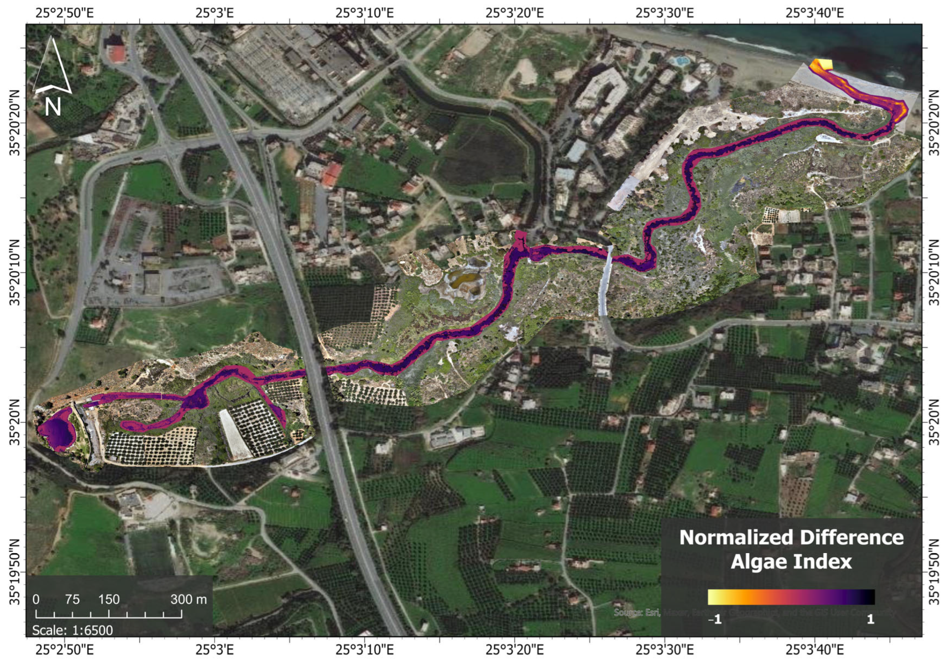
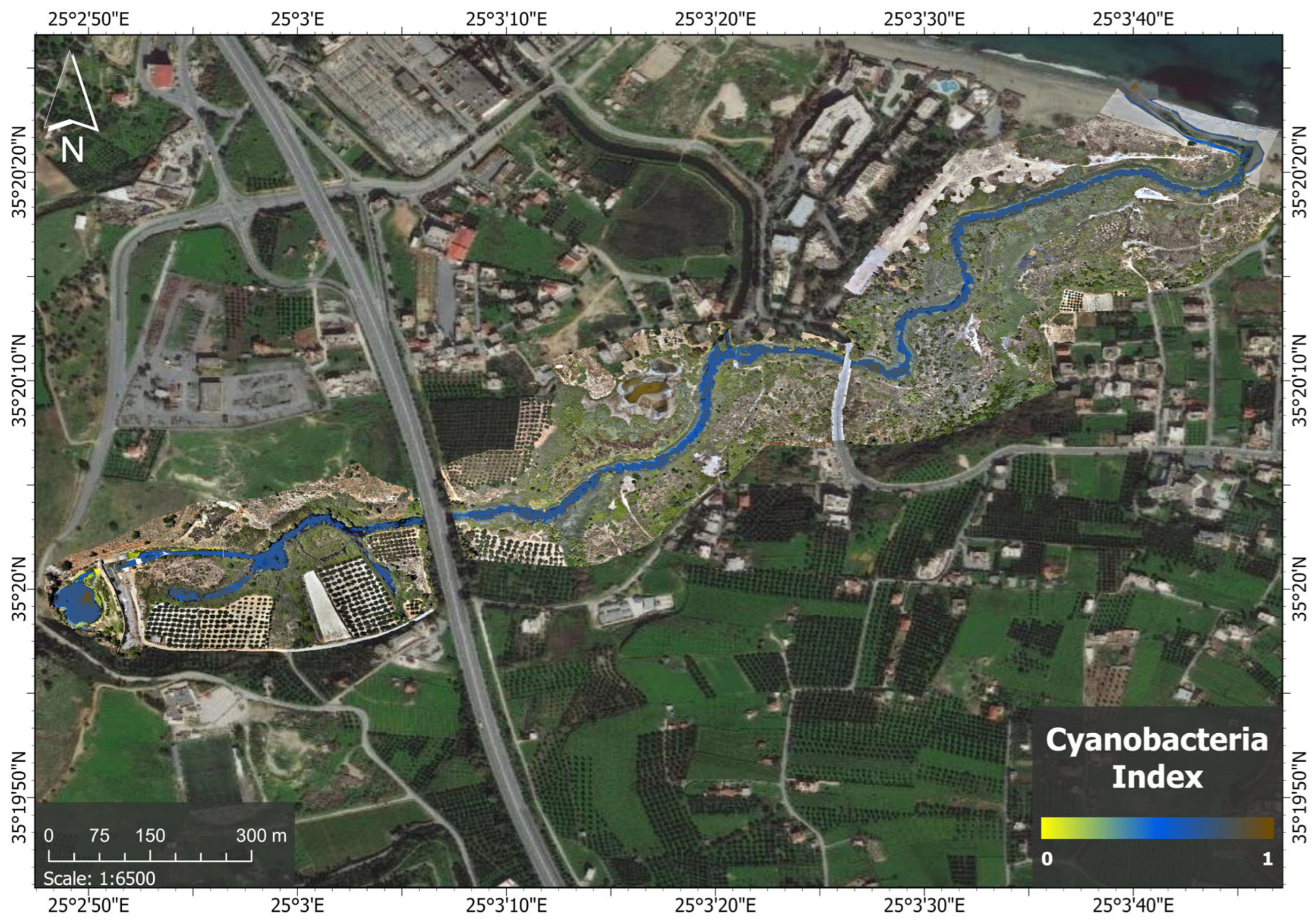
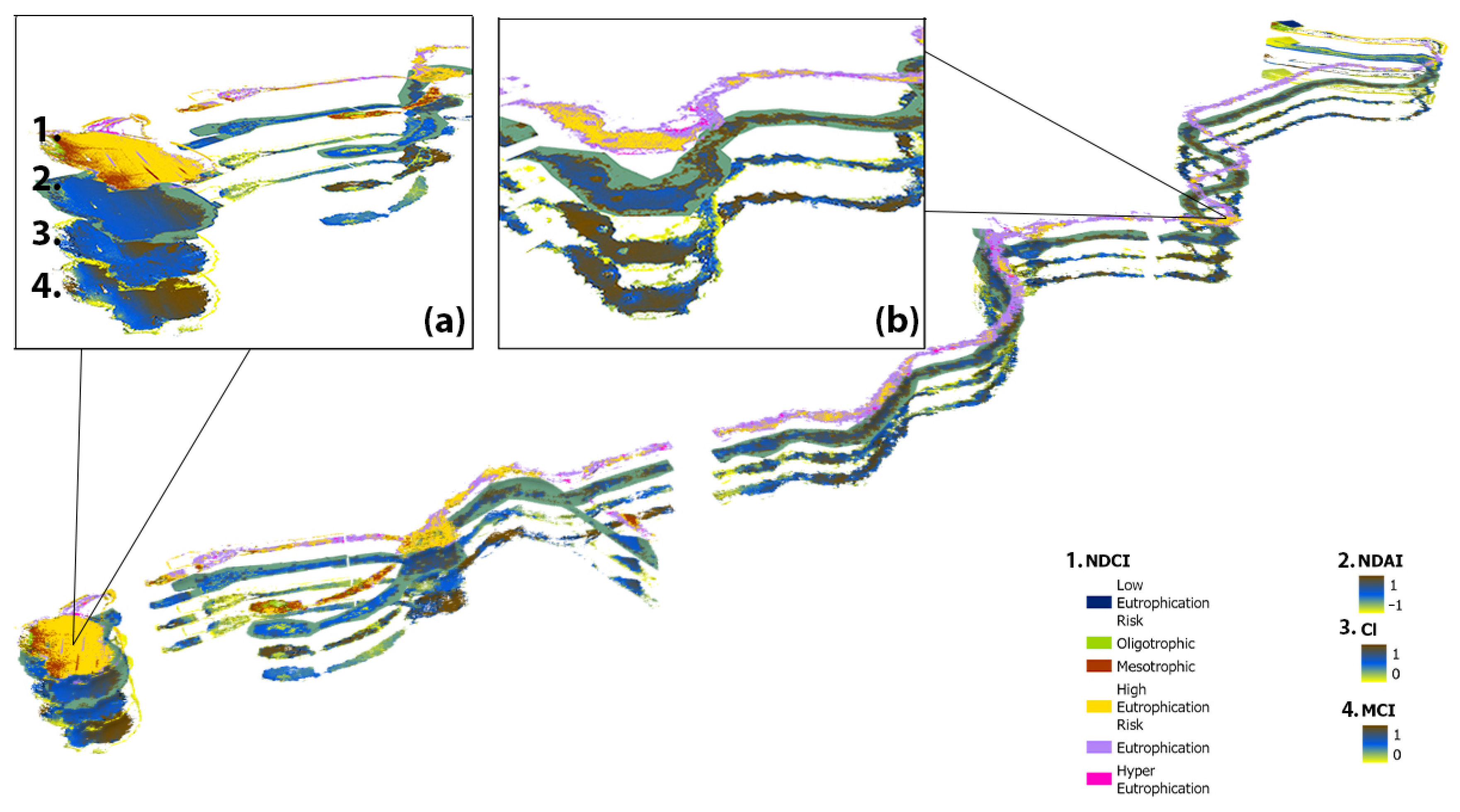
3.1.1. Water Indices
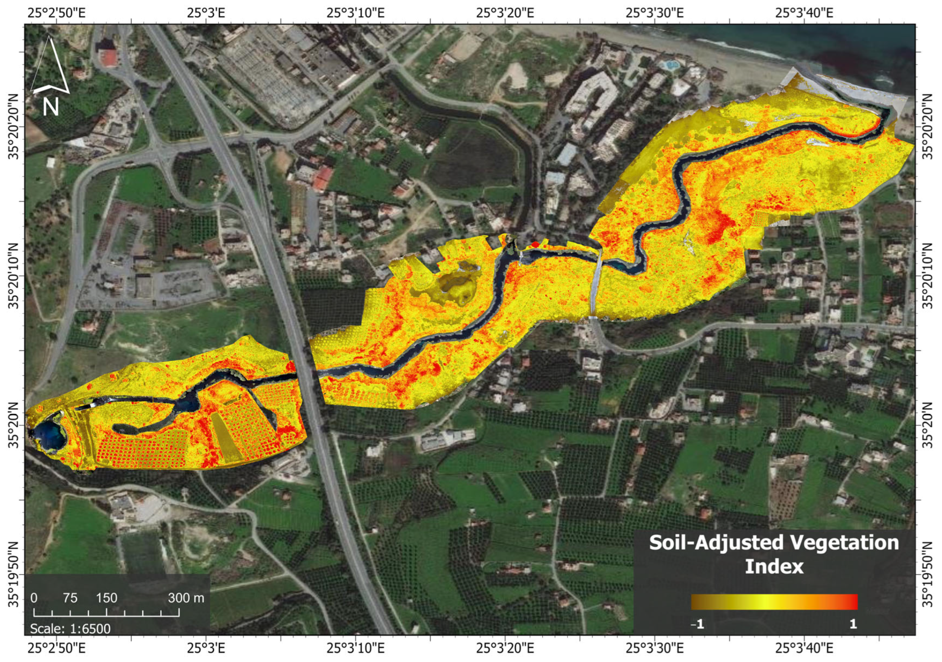
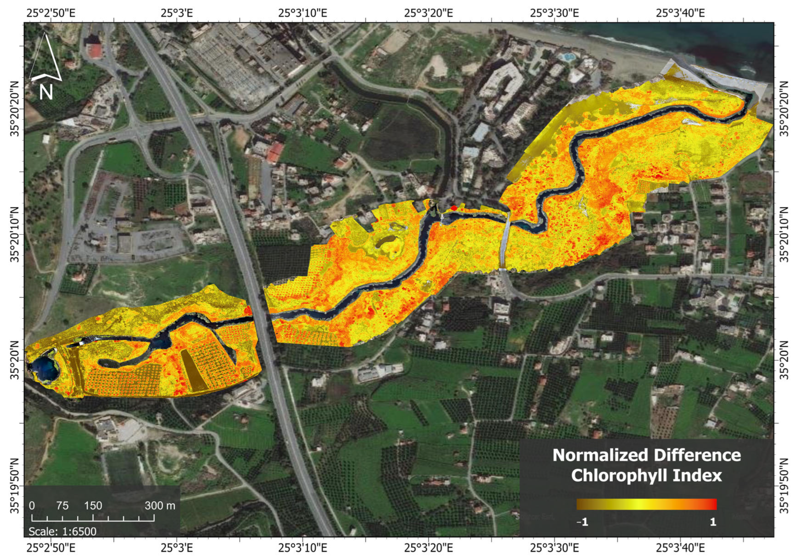
3.1.2. Land and Soil Indices
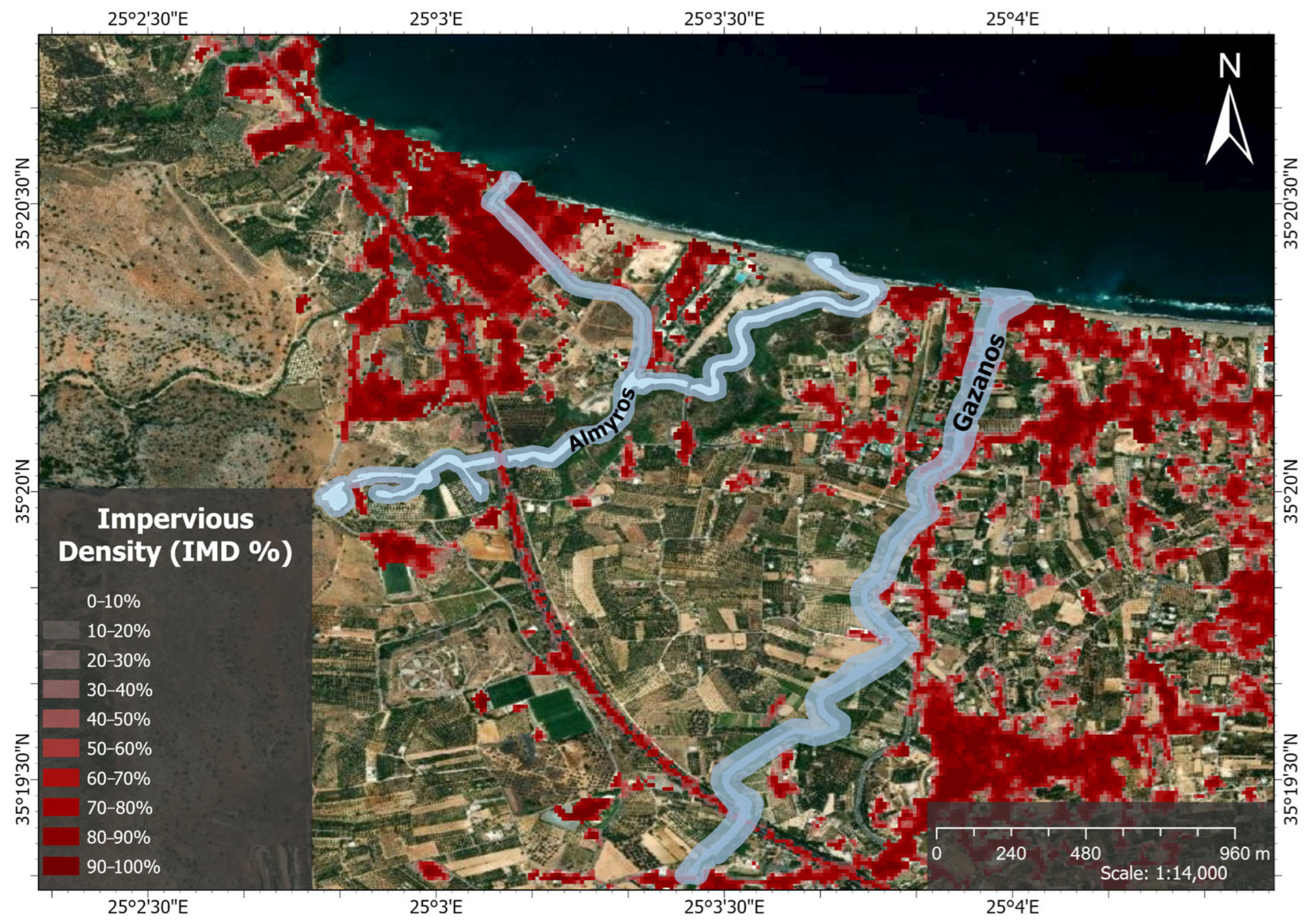
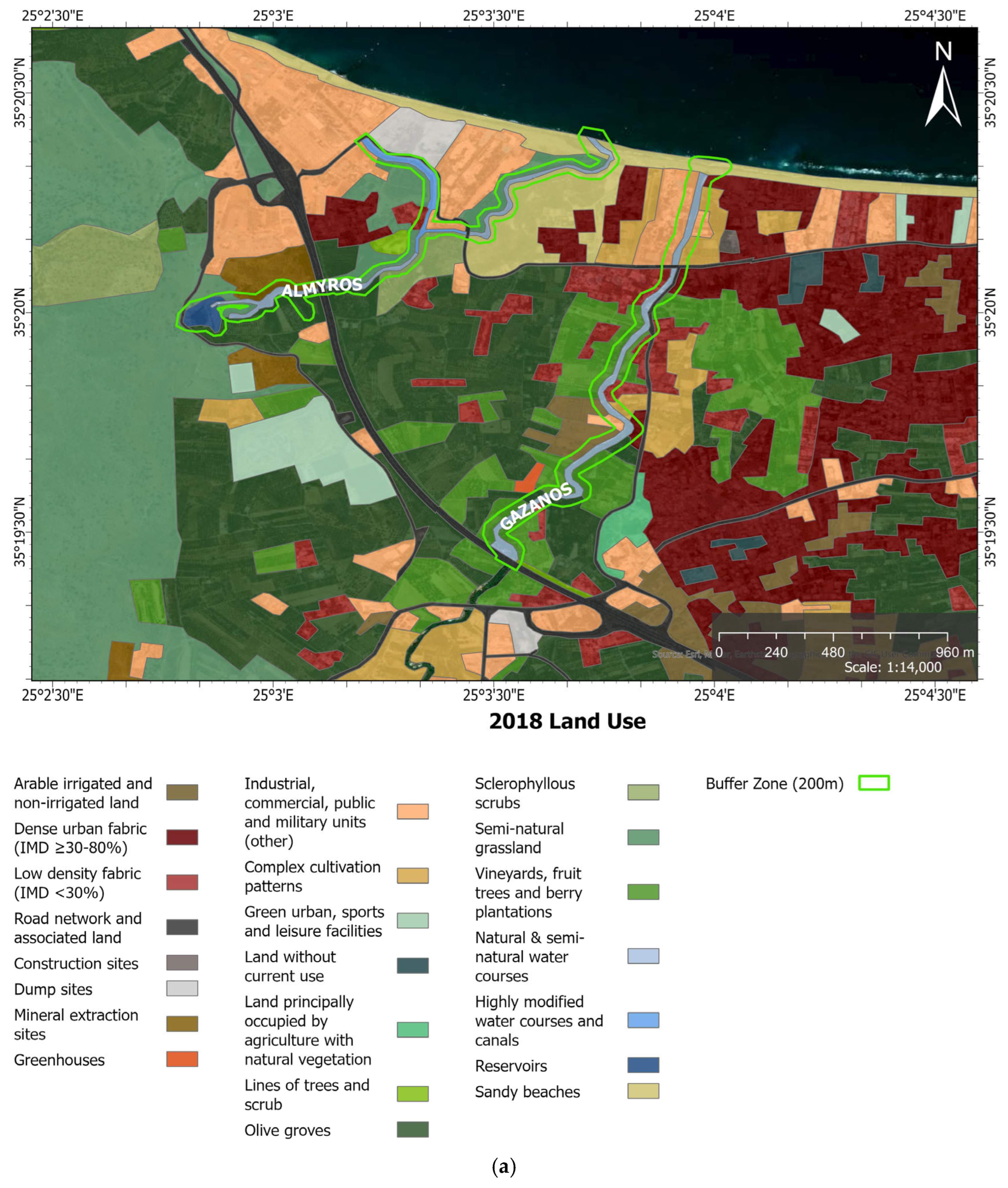
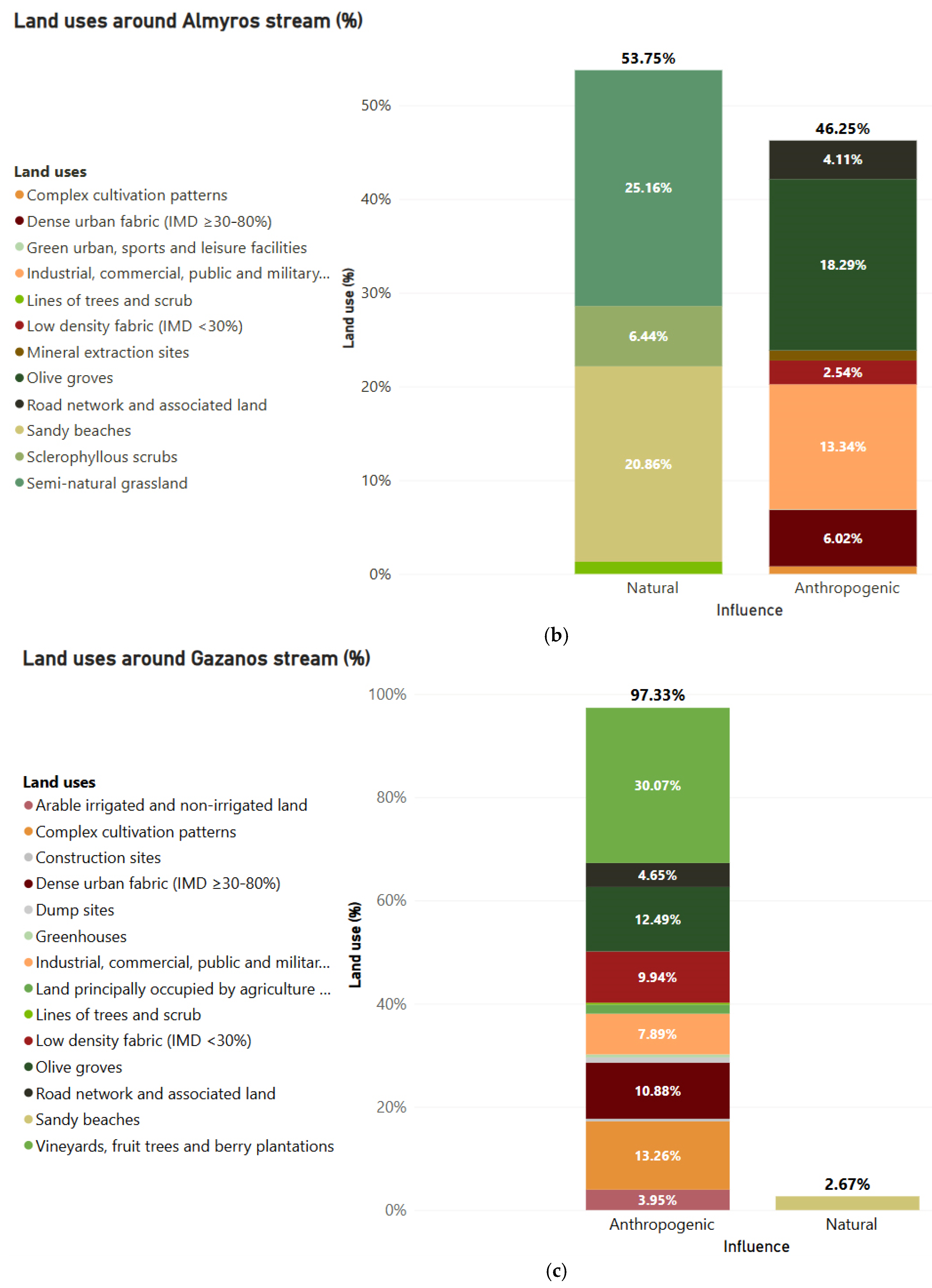
3.2. Land Use
3.3. Geophysical and Physicochemical Evaluation
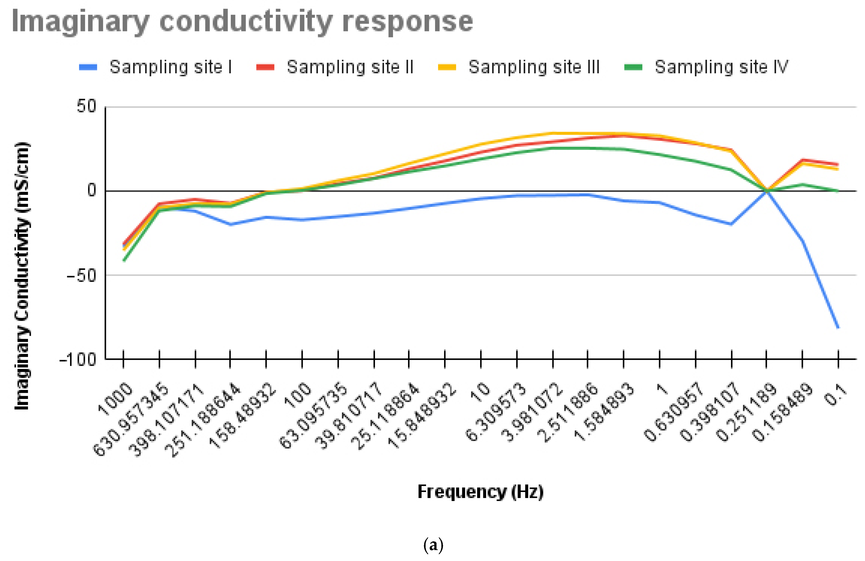
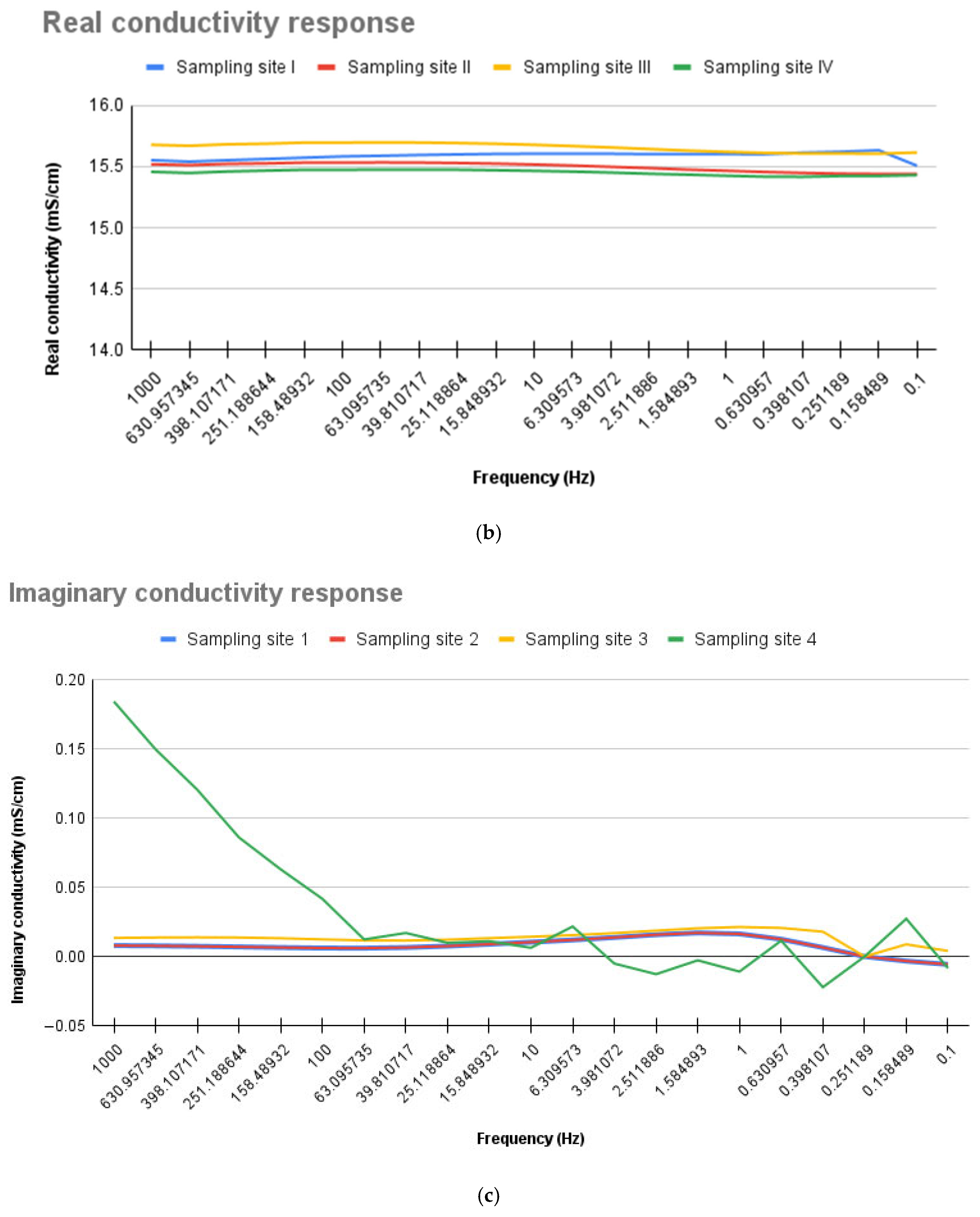
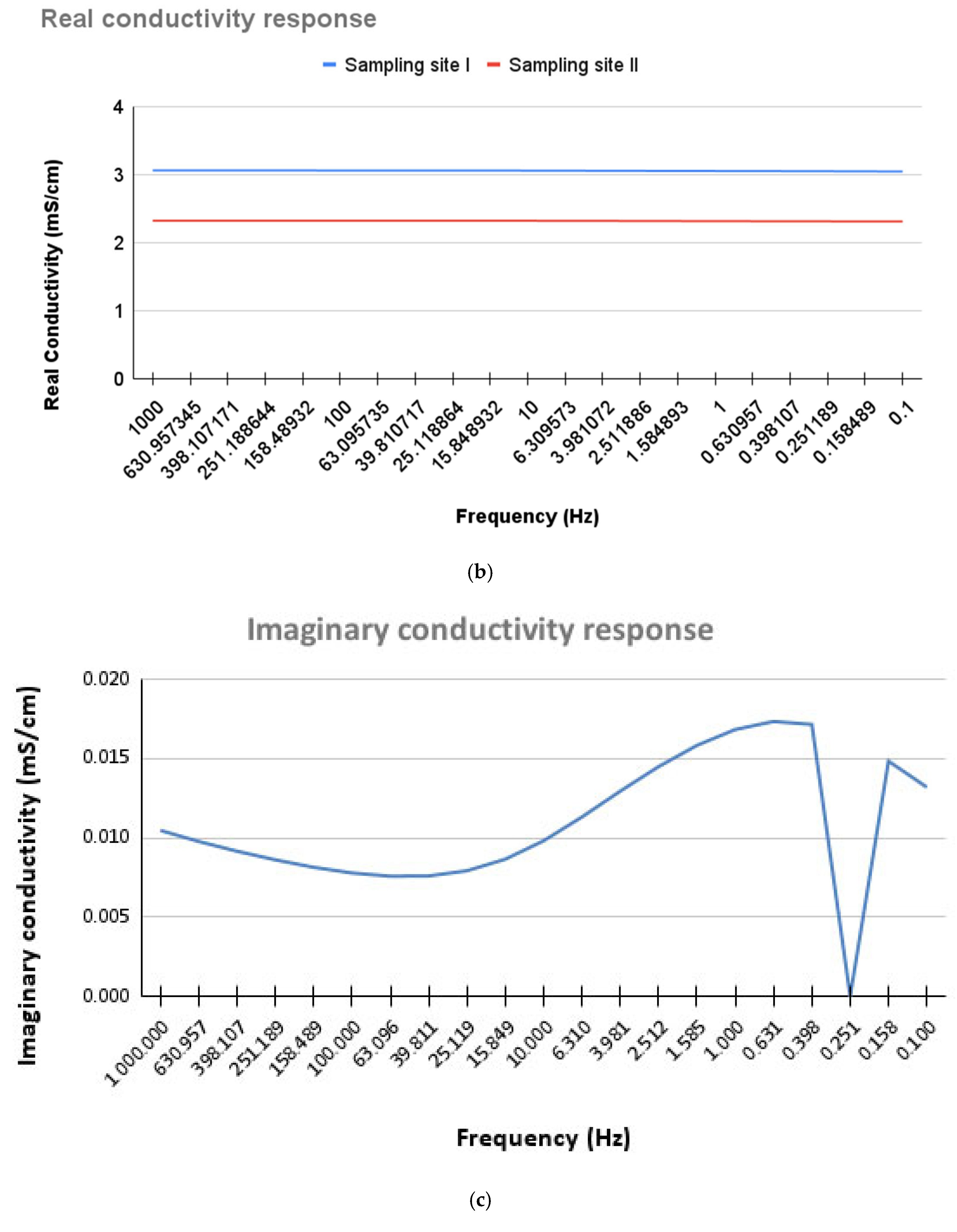
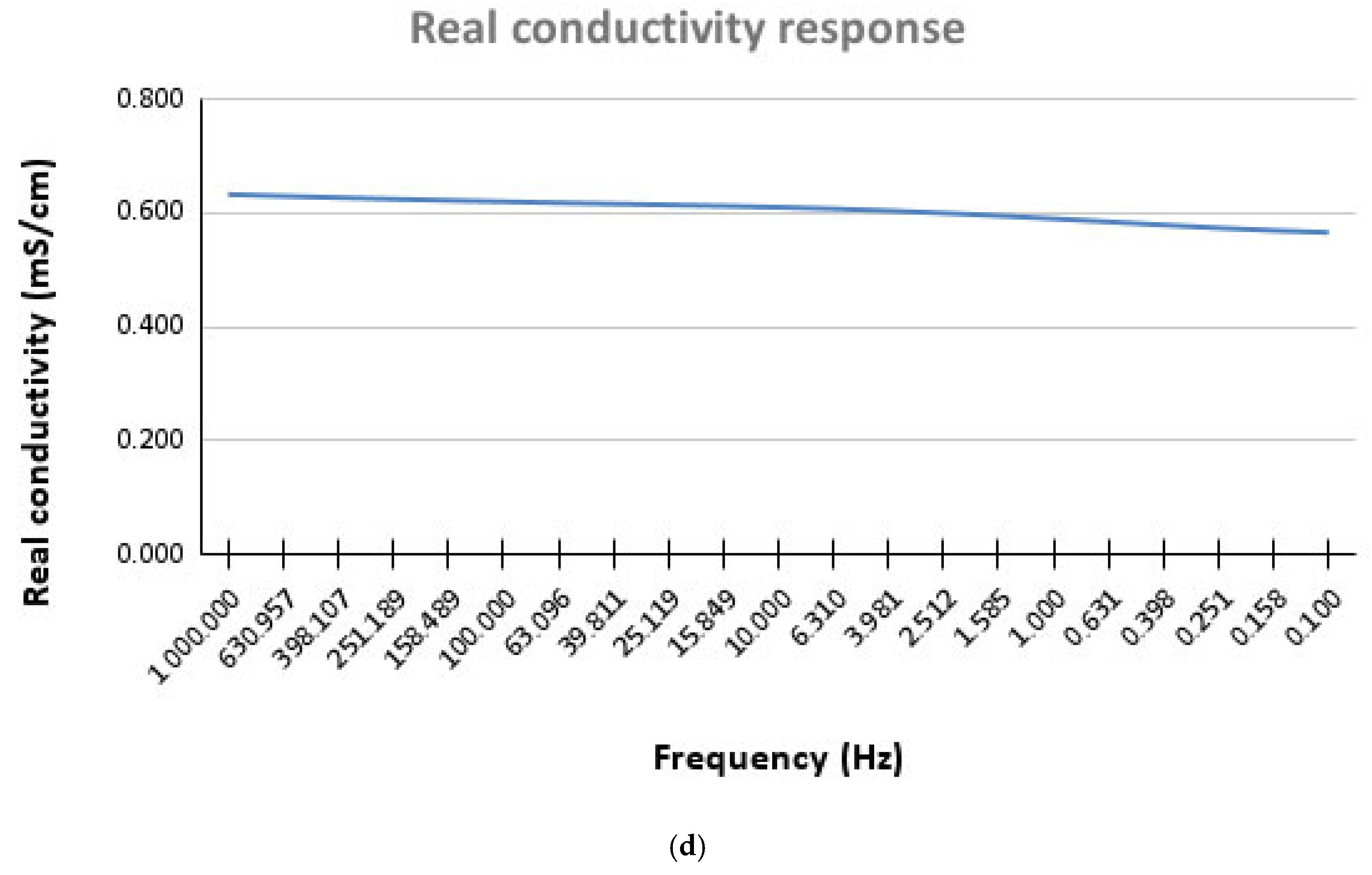
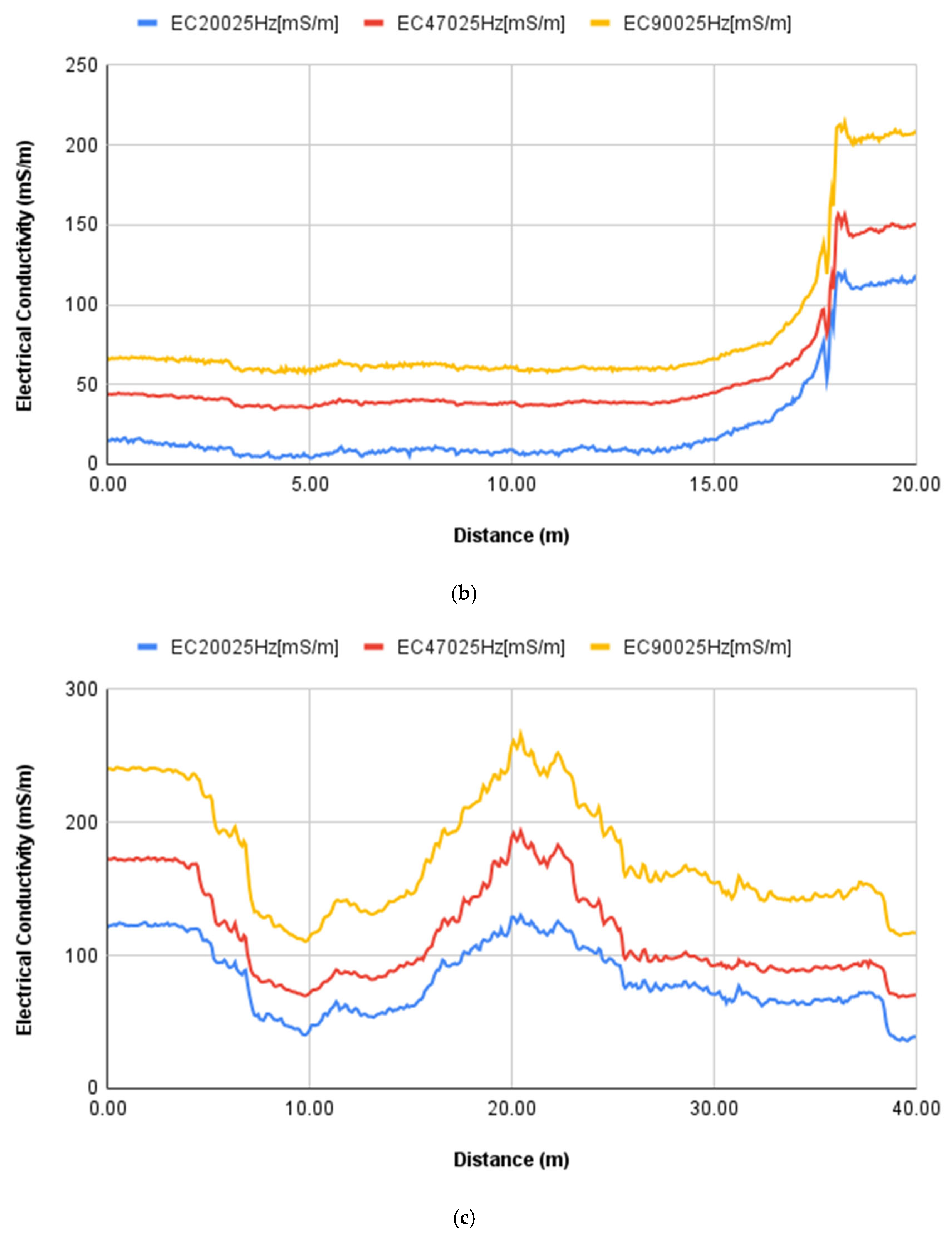
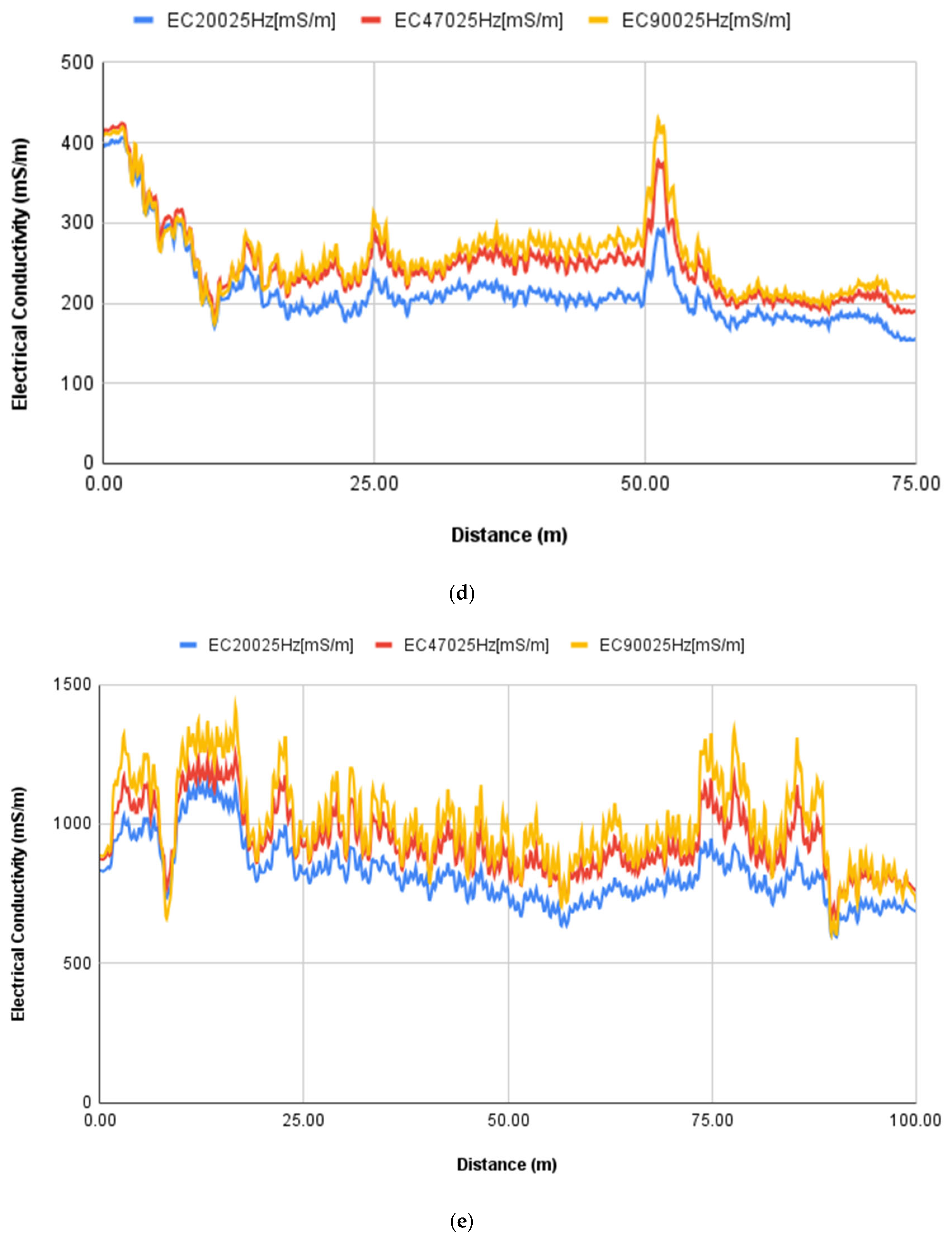
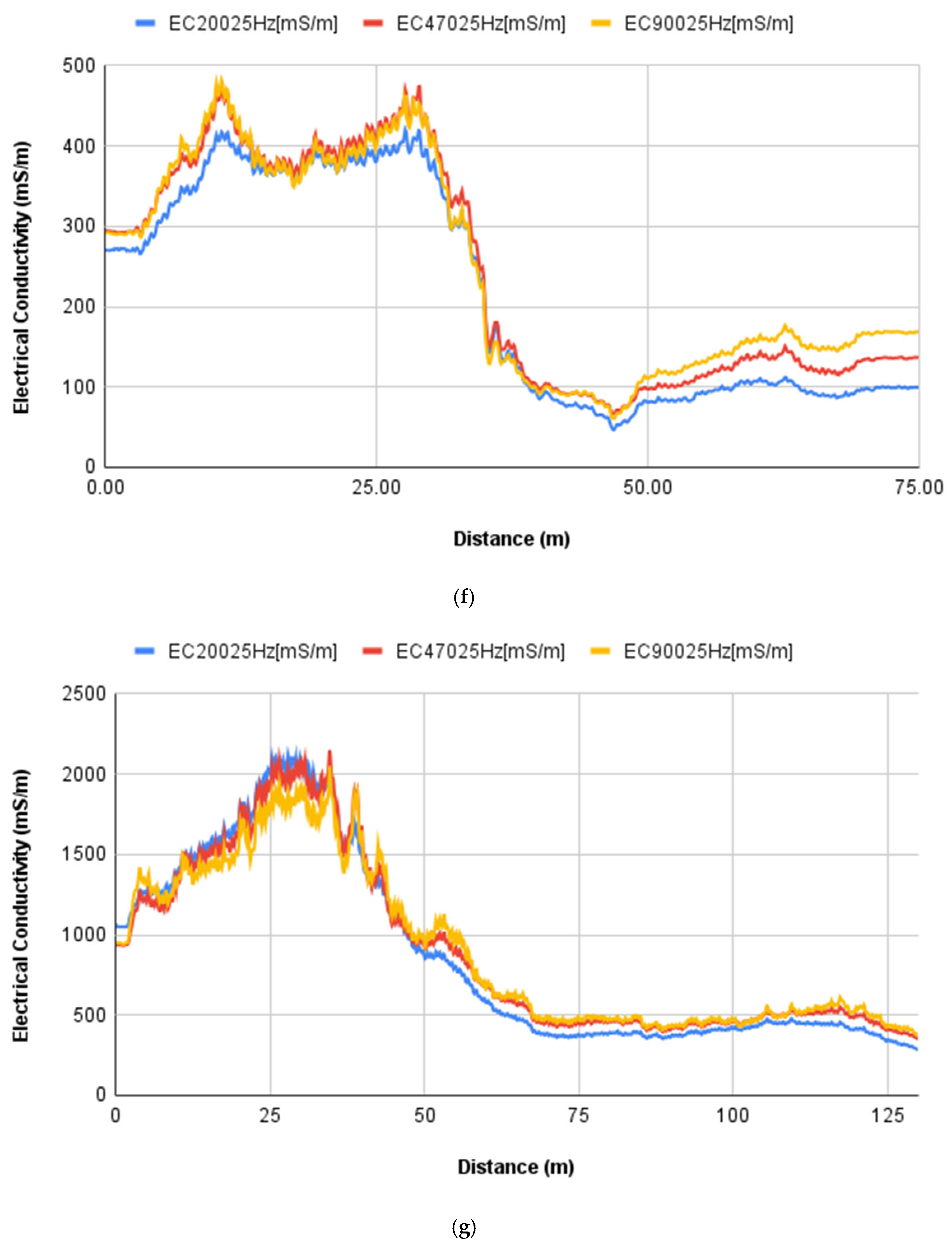
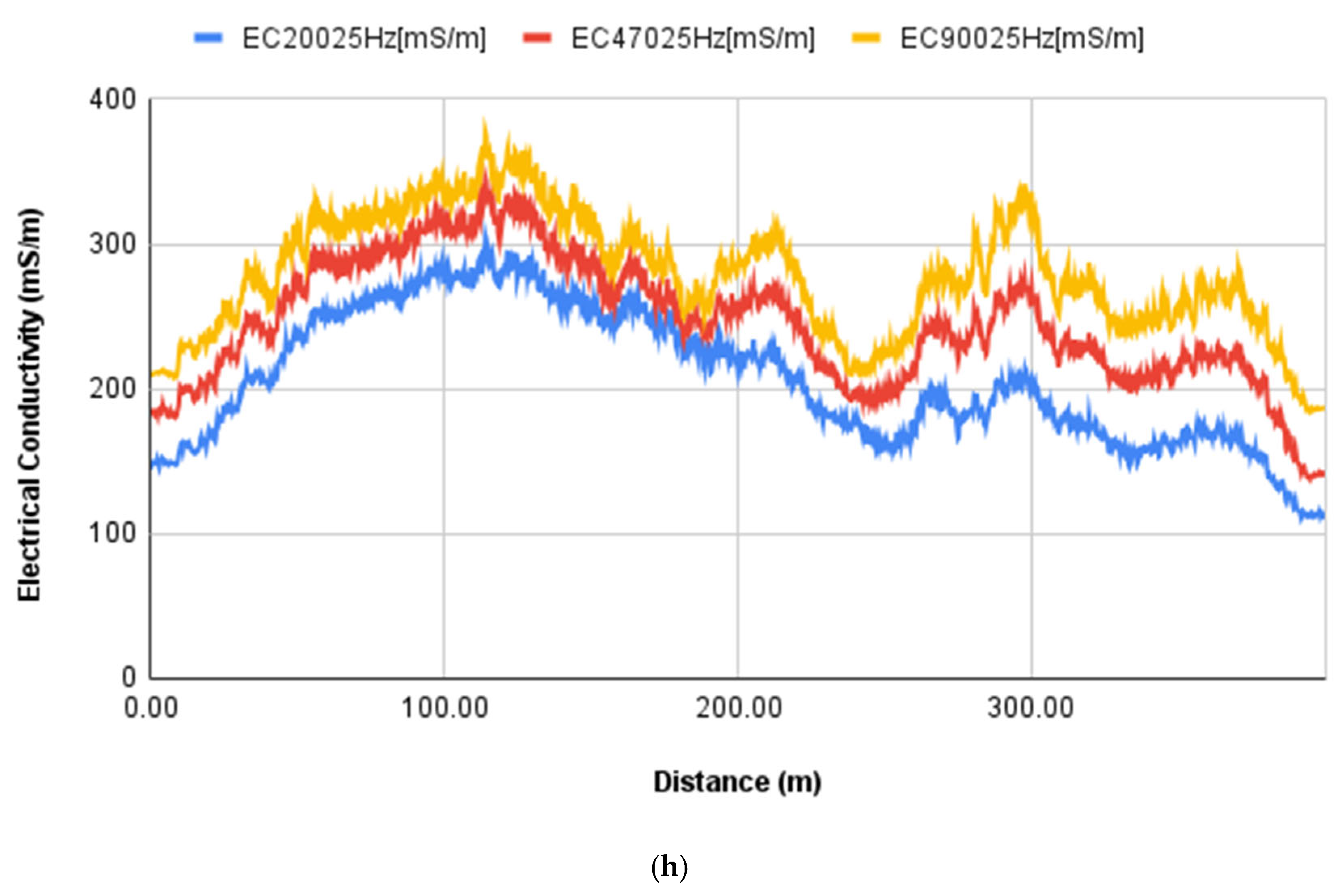
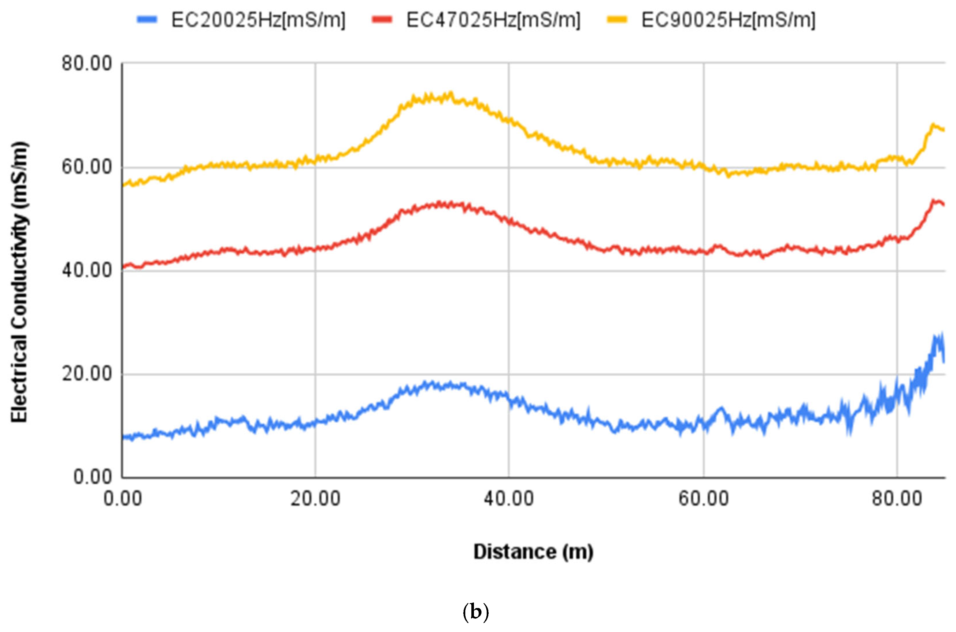
Geophysical Measurements
3.4. Chemical Analysis
4. Discussion
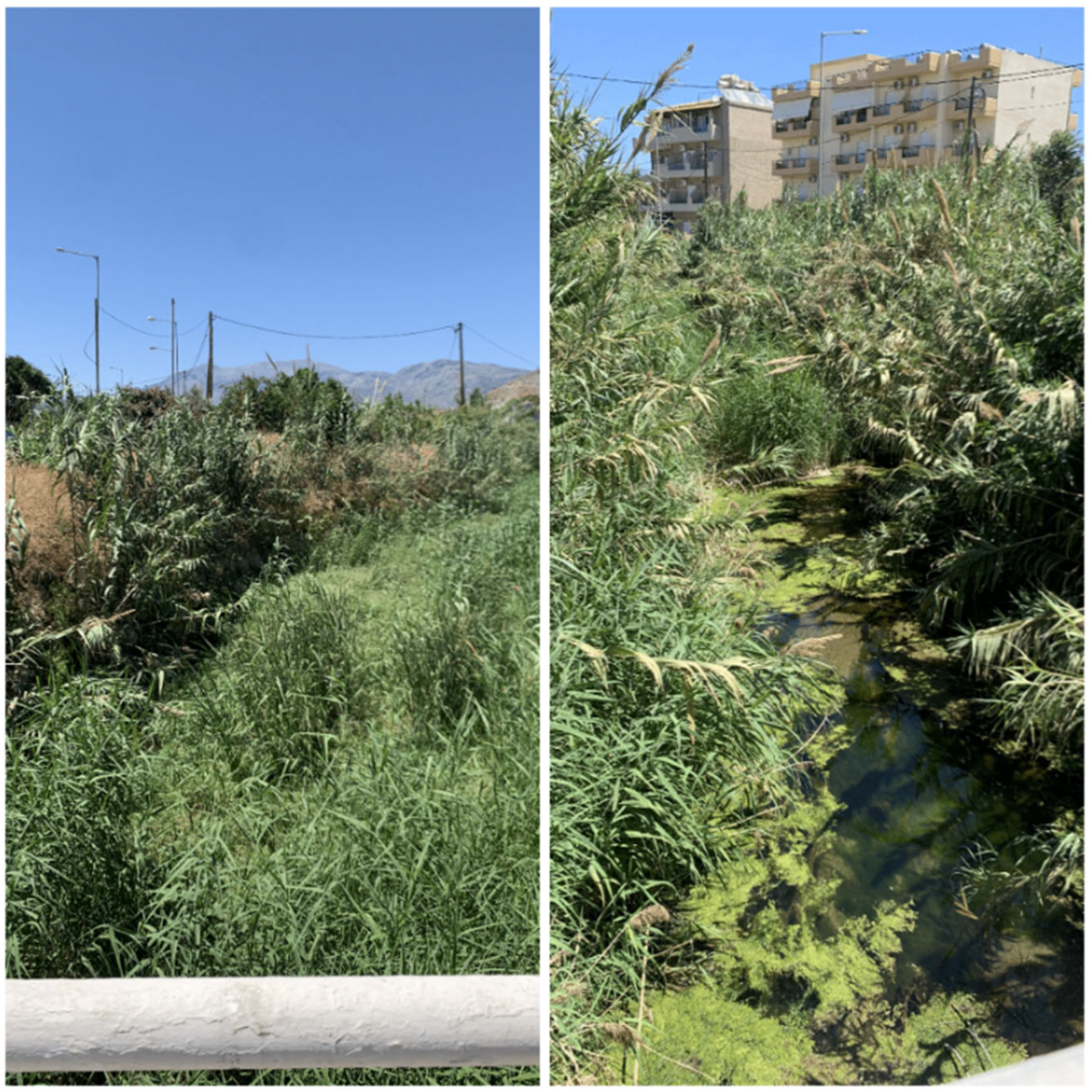
4.1. Almyros Stream: Eutrophication and Algal Blooms
4.2. Gazanos Stream: Impact of Urbanization
4.3. Combined Monitoring Approach
5. Conclusions
- Combined Monitoring Approach: This study successfully demonstrates the effectiveness of combining RS techniques, including satellite and drone imagery, with in situ measurements such as Spectral Induced Polarization (SIP), GEM-2, and chemical analyses. This combination provides a comprehensive, multi-dimensional evaluation of the health of urban streams, critical for timely and accurate assessments (Table A3, Appendix A). We recommend the creation of a dashboard that presents comprehensive data from longitudinal studies.
- Ecosystem Health Insights: The research findings highlight that the Almyros stream is experiencing significant eutrophication, as indicated by high chlorophyll levels and algal blooms primarily due to agricultural runoff. On the other hand, the Gazanos stream, while not classified as eutrophic, is burdened by pollution resulting from urbanization.
- Importance of Land Use Analysis: Analysis of land use surrounding the streams indicated that agricultural practices significantly impact the Almyros stream, accounting for over 40% of the influencing factors. Conversely, the Gazanos stream is heavily influenced by urban development, which comprises 90% of the land use in its vicinity. This finding highlights the critical need to understand local land use impacts for effective stream health assessments.
- Role of Geophysical and Chemical Assessments: The combination of RS data with SIP, GEM-2, and chemical assessments provides valuable insights into subsurface conditions and contaminant distribution. Geophysical and chemical assessments improved the precision of pollution detection and the understanding of its sources, aiding in more effective management interventions.
- Call for Ongoing Monitoring: There is an urgent need for continuous monitoring programs that use integrated approaches to track changes in stream condition over time. Regular data collection using both RS and in situ methods can facilitate the development of early warning systems to detect ecological degradation and enable timely interventions to protect urban aquatic ecosystems.
Author Contributions
Funding
Data Availability Statement
Acknowledgments
Conflicts of Interest
Appendix A

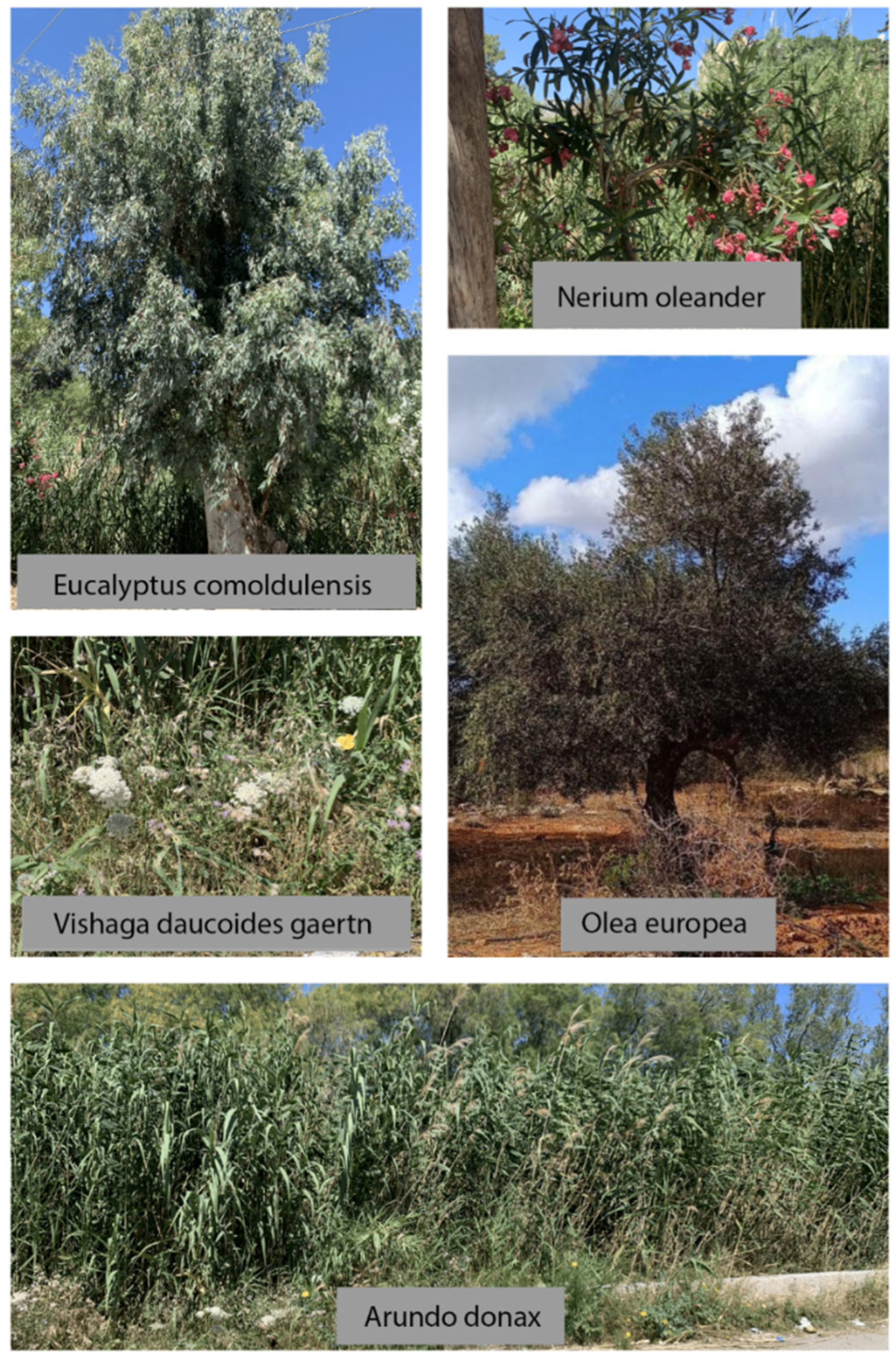
| Plant Name | Plant Type | Description |
|---|---|---|
| Eucalyptus sp. | Perennial tree | Known for rapid growth and adaptability |
| Olea europea | Perennial tree | Cultivated for olives and oil; a long-lived Mediterranean species |
| Ceratonia siliqua | Perennial tree | Known as Carob, which is drought tolerant |
| Tamarix sp. | Perennial shrub/tree | Salt-tolerant; invasive in some regions, used for soil stabilization |
| Phoenix theophrasti | Perennial palm | Endemic to Crete, drought tolerant |
| Rhamus alaternus | Perennial shrub | Evergreen shrub |
| Acacia retinodes | Perennial tree | Known as Swamp Wattle; ornamental and drought tolerant |
| Nerium oleander | Perennial shrub | Toxic evergreen shrub, used in landscaping |
| Euphorbia characias | Perennial shrub | Drought-tolerant with unique floral structures; commonly ornamental |
| Urticia dioica | Perennial herbaceaous | Stinging nettle; used in herbal medicine and as a food source |
| Nicotina glauca | Perennial shrub | Tree tobacco: invasive in some areas, thrives in arid regions |
| Drimia maritima | Perennial herbaceous | Known as Sea Squill; medicinal and ornamental uses |
| Phragmites australis | Perennial grass | Common reed, used in water filtration and habitat restoration |
| Eryngium maritimum | Perennial herbaceous | Sea holly, ornamental coastal plant with blue spiky flowers |
| Glebionis coronaria | Annual herbaceous | Garland chrysanthemum, edible leaves used in Mediterranean cuisine |
| Glycyrrhiza glabra | Perennial herbaceous | Licorice plant: roots used for flavoring and medicinal purposes |
| Carex pseudocyperus | Perennial sedge | Found in wet habitats; used in erosion control and habitat restoration |
| Capparis spinosa | Perennial shrub | Caper bush, edible flower buds are used in cooking. |
| Cota tinctoria | Perennial herbaceous | Dyer’s chamomile; used historically in dyeing fabrics |
| Matricaria chamomilla | Annual herbaceous | German chamomile. |
| Salicornia europea | Annual herbaceous | Known as glasswort; thrives in saline conditions, edible shoots |
| Ricinus communis | Perennial shrub/tree | Castor bean plant: seeds produce castor oil, highly toxic |
| Cakile maritime | Annual herbaceous | Sea rocket, edible coastal plant adapted to saline soils |
| Sonchus oleraceus | Annual herbaceous | Sow thistle, a fast-growing weed used for fodder and human consumption |
| Visnaga daucoides | Biennial herbaceous | Medicinal plant |
| Arundo donax | Perennial shrub | Giant Reed: invasive in some regions, used for biomass and erosion control |
| Galactites tomentosus | Annual Herbaceous | Ornamental thistle, native of the Mediterranean |
| Plant Name | Plant Type | Description |
|---|---|---|
| Robinia hispida | Perennial shrub | Also called Bristly Locust; nitrogen-fixing and used for erosion control. Adapted to various soils and climates |
| Glaucium flavum | Perennial herbaceous | Known as Yellow Horned Poppy; drought-tolerant coastal plant with medicinal uses |
| Arundo donax | Perennial grass | Giant Reed: Invasive in some regions, used for biomass and erosion control. |
| Visnaga daucoides | Biennial herbaceous | It has a history of being used both as food and poison |
| Ecballium elaterium | Perennial herbaceous | Known as squirting Cucumber: grows in arid conditions, noted for its medicinal properties but toxic if ingested |
| Ficus benjamina | Perennial tree | Known as Weeping Figure, a popular indoor plant that thrives in tropical and subtropical climates |
| Nerium oleander | Perennial shrub | Evergreen shrub, toxic, commonly used in landscaping |
| Eucalyptus camaldulensis | Perennial tree | River Red Gum: fast-growing, thrives in dry regions, often planted for timber and erosion control |
| Pandorea jasminoides | Perennial vine | Jasmine-like flowering vine, popular in ornamental horticulture |
| Ricinus communis | Perennial shrub/tree | Castor Bean Plant: seeds yield castor oil, though highly toxic |
| Eucalyptus sp. | Perennial tree | Known for rapid growth and adaptability |
| Olea europea | Perennial tree | Cultivated for olives and oil; a long-lived Mediterranean species |
| Water Indices and Formula | Soil Indices and Formula | Geophysical indicators | Chemical Analyses | ||
|---|---|---|---|---|---|
| Physicochemical Parameters | Nutrients and Pigments | ||||
| Normalized Difference Chlorophyll Index (RE1 − R)/(RE1 + R) | Soil Adjusted Vegetation Index (1.0 + L) × (N − R)/(N + R + L) | Real conductivity (SIP) | pH | Nitrogen | |
| Normalized Difference Algae Index (NIR − R)/(NIR + R) | Green Normalized Difference Vegetation Index (N − G)/(N + G) | Imaginary conductivity (SIP) | Temperature | Phosphorus | |
| Maximum Chlorophyll Index RE − (N + (N + RE) * (RE − R/N − R)) | Normalized Difference Chlorophyll Index (RE1 − R)/(RE1 + R) | Apparent Conductivity (GEM-2) | Conductivity | Ammonium | |
| Cyanobacteria Index RE − (G + (N − G) * (RE − G/N − G) | Dissolved Oxygen | Chlorophyll-a | |||
| Carotenoids | |||||
| Aluminum dissolved | Chromium dissolved | Mercury dissolved | HCO3 |
| Arsenic dissolved | Copper dissolved | Nickel dissolved | Nitrate |
| Cadmium dissolved | Dissolved oxygen | Potassium | Nitrite |
| Calcium | Iron dissolved | Sodium | Total phosphates |
| Carbonates | Lead dissolved | Sulphate | |
| Chloride | Magnesium | Zinc dissolved | |
| Chromium 6+ | Manganese dissolved | Ammonium |
| 1,1-Dichloroethene | 1,1,1-Trichloroethane | 1,1,2-Trichloroethane | 1,1,2,2-Tetrachloroethene | 1,2-Dichlorobenzene | 1,2-Dichloroethene | 1,2-Dichloroethane | 1,3-Dichlorobenzene |
| 1,4-Dichlorobenzene | 2-Chlorotoluene | 2,2′,3,3′,4,4′-Hexachlorobiphenyl | 2,2′,3,4,4′,5-Hexachlorobiphenyl | 2,2′,3,4,4′,5,6-Heptachlorobiphenyl | 2,2′,3,4,5-Pentachlorobiphenyl | 2,4-D | 2,4,5-T |
| 3,4-Dichloroaniline | 4-Chloroaniline | 4-Chlorotoluene | 4-Nonylphenol | Aclonifen | Alachlor | Aldrin | Alpha-Endosulfan |
| Alpha-HCH | Ammonium | Anthracene | Arsenic | Atrazine | Azinphos ethyl | Azinphos methyl | Bentazone |
| Benzene | Benzo(a)pyrene | Benzo(b)fluoranthene | Benzo(g,h,i)perylene | Benzo(k)fluoranthene | Beta-Endosulfan | Beta-HCH | Bifenox |
| BOD5 | Cadmium | Chlorfenvinphos | Chloridazon | Chlorobenzene | Chlorpyrifos | Chromium | Chromium 6+ |
| Cis-1,2-Dichloroethene | Cl | Cobalt and its compounds | Copper | Coumaphos | Cyanides (as total CN) | Cybutryne | Cyclodiene total |
| Cypermethrin | DDD, p,p″ | DDE, p,p″ | DDT total | DDT, o,p″ | DDT, p,p″ | Delta-HCH | Demeton O+S |
| Demeton-S-Methyl | Detergents | Di(2-ethylhexyl) phthalate (DEHP) | Dichloromethane | Dichlorprop (2,4-DP) | Dichlorvos | Dicofol | Dieldrin |
| Dimethoate | Dissolved Oxygen | Disulfoton | Diuron | Endosulfan | Endrin | Ethylbenzene | Fenitrothion |
| Fenthion | Fluoranthene | Gamma-HCH (Lindane) | Heptachlor | Heptachloroepoxide | Hexachlorobutadiene (HCBD) | Hexachlorocyclohexane (HCH) | InvertebrateEQR |
| Isodrin | Isoproturon | Lead | Linuron | M-Xylene | Malathion | MCPA | Mecoprop |
| Mercury | Meta + Para Xylene | Methamidophos | Mevinphos | Molybdenum and its compounds | Monolinuron | Naphthalene | Nickel |
| Nitrate | Nitrite | O-Xylene | Omethoate | Orthophosphates | Oxydemeton-Methyl | P-Xylene | Para-tert-Octylphenol |
| Parathion | Parathion-Methyl | PCB’s Total | PCB101 (2,2′,4,5,5′-Pentachlorobiphenyl) | PCB105 (2,3,3′,4,4′-Pentachlorobiphenyl) | PCB114 (2,3,4,4′,5-Pentachlorobiphenyl) | PCB153 (2,2′,4,4′,5,5′-Hexachlorobiphenyl) | PCB156 (2,3,3′,4,4′,5-Hexachlorobiphenyl) |
| PCB169 | PCB170 | PCB180 | PCB194 | PCB28 | PCB52 | Pentachlorophenol | PFOS |
| Phenol | Phenols | Propanil | Quinoxyfen | Selenium and its compounds | Simazine | Terbutryn | Tetrachloromethane |
| Tin and its compounds | Toluene | Total Dissolved Solids | Total Phosphorus | Trans-1,2-Dichloroethene | Triazophos | Tributyltin | Trichlorfon |
| Trichloromethane | Trifluralin | Zinc |
References
- Gunawardena, K.R.; Wells, M.J.; Kershaw, T. Utilising green and bluespace to mitigate urban heat island intensity. Sci. Total Environ. 2017, 584–585, 1040–1055. [Google Scholar] [CrossRef] [PubMed]
- United Nations. 68% of the World Population Projected to Live in Urban Areas by 2050, Says UN. Available online: https://www.un.org/uk/desa/68-world-population-projected-live-urban-areas-2050-says-un (accessed on 19 September 2024).
- Ritchie, H.; Samborska, V.; Roser, M. Urbanization. Our World Data 23 February 2024. Available online: https://ourworldindata.org/urbanization (accessed on 19 September 2024).
- Roy, A.H.; Paul, M.J.; Wenger, S.J. Urban Stream Ecology. In Urban Ecosystem Ecology; Aitkenhead-Peterson, J., Volder, A., Eds.; Wiley: Hoboken, NJ, USA, 2010; pp. 341–352. [Google Scholar] [CrossRef]
- Paul, M.J.; Meyer, J.L. Streams in the urban landscape. Annu. Rev. Ecol. Syst. 2001, 32, 333–365. [Google Scholar] [CrossRef]
- Gilliom, R.; Barbash, J.; Crawford, C.; Hamilton, P.; Martin, J.; Nakagaki, N.; Nowell, L.H.; Scott, J.C.; Stackelberg, P.E.; Thelin, G.P.; et al. The Quality of Our Nation’s Waters—Pesticides in the Nation’s Streams and Ground Water, 1992–2001; U.S. Geological Survey: Reston, VA, USA, 2006; 172p.
- Marti, E.; Aumatell, J.; Godé, L.; Poch, M.; Sabater, F. Nutrient retention efficiency in streams receiving inputs from wastewater treatment plants. J. Environ. Qual. 2004, 33, 285–293. [Google Scholar] [CrossRef]
- Booth, D.B.; Jackson, C.R. Urbanization of aquatic systems: Degradation, thresholds, stormwater detection, and the limits of mitigation. J. Am. Water Resour. Assoc. 1997, 33, 1077–1090. [Google Scholar] [CrossRef]
- Wolman, M.G.; Schick, A.P. Effects of construction on fluvial sediment, urban and suburban areas of Maryland. Water Resour. Res. 1967, 3, 451–464. [Google Scholar] [CrossRef]
- Walsh, C.J.; Roy, A.H.; Feminella, J.W.; Cottingham, P.D.; Groffman, P.M.; Morgan, R.P. The urban stream syndrome: Current knowledge and the search for a cure. J. N. Am. Benthol. Soc. 2005, 24, 706–723. [Google Scholar] [CrossRef]
- Catford, J.A.; Jansson, R.; Nilsson, C. Reducing redundancy in invasion ecology by integrating hypotheses into a single theoretical framework. Divers. Distrib. 2009, 15, 22–40. [Google Scholar] [CrossRef]
- Potapova, M.; Charles, D. Choice of substrate in algae-based water-quality assessment. J. N. Am. Benthol. Soc. 2005, 24, 415–427. [Google Scholar] [CrossRef]
- Aliyas, Z. Physical, mental, and physiological health benefits of green and blue outdoor spaces among elderly people. Int. J. Environ. Health Res. 2021, 31, 703–714. [Google Scholar] [CrossRef]
- Garrett, J.K.; White, M.P.; Huang, J.; Ng, S.; Hui, Z.; Leung, C.; Tse, L.A.; Fung, F.; Elliott, L.R.; Depledge, M.H.; et al. Urban blue space and health and wellbeing in Hong Kong: Results from a survey of older adults. Health Place 2019, 55, 100–110. [Google Scholar] [CrossRef]
- Pearson, A.L.; Shortridge, A.; Delamater, P.L.; Horton, T.H.; Dahlin, K.; Rzotkiewicz, A.; Marchiori, M.J. Effects of freshwater blue spaces may be beneficial for mental health: A first, ecological study in the North American Great Lakes region. PLoS ONE 2019, 14, e0221977. [Google Scholar] [CrossRef] [PubMed]
- Liang, Y.; Ding, F.; Liu, L.; Yin, F.; Hao, M.; Kang, T.; Zhao, C.; Wang, Z.; Jiang, D. Monitoring water quality parameters in urban rivers using multi-source data and machine learning approach. J. Hydrol. 2025, 648, 132394. [Google Scholar] [CrossRef]
- Liu, C.; Zhou, X.; Zhou, Y.; Akbar, A. Multi-temporal monitoring of urban river water quality using UAV-borne multi-spectral remote sensing. In The International Archives of the Photogrammetry, Remote Sensing and Spatial Information Sciences, XLIII-B3-2020; Copernicus GmbH: Göttingen, Germany, 2020; pp. 1469–1475. [Google Scholar] [CrossRef]
- Gong, C.; Li, L.; Hu, Y.; Wang, X.; He, Z.; Wang, X. Urban river water quality monitoring with unmanned plane hyperspectral remote sensing data. In Seventh Symposium on Novel Photoelectronic Detection Technology and Application 2020; Chu, J., Yu, Q., Jiang, H., Su, J., Eds.; SPIE: Nuremberg, Germany, 2020; p. 67. [Google Scholar] [CrossRef]
- Zheng, Z.; Jiang, Y.; Zhang, Q.; Zhong, Y.; Wang, L. A feature selection method based on relief feature ranking with recursive feature elimination for the inversion of urban river water quality parameters using multispectral imagery from an unmanned aerial vehicle. Water 2024, 16, 1029. [Google Scholar] [CrossRef]
- Chen, B.; Mu, X.; Chen, P.; Wang, B.; Choi, J.; Park, H.; Xu, S.; Wu, Y.; Yang, H. Machine learning-based inversion of water quality parameters in typical reach of the urban river by UAV multispectral data. Ecol. Indic. 2021, 133, 108434. [Google Scholar] [CrossRef]
- Zhang, Y.; Yang, Z. Retrieve water quality parameters of urban rivers from hyperspectral images through feature interaction based two-stage method fused with spectral unmixing and spatial relatedness. Sci. Total Environ. 2024, 956, 177115. [Google Scholar] [CrossRef] [PubMed]
- Chen, P.; Wang, B.; Wu, Y.; Wang, Q.; Huang, Z.; Wang, C. Urban river water quality monitoring based on self-optimizing machine learning method using multi-source remote sensing data. Ecol. Indic. 2023, 146, 109750. [Google Scholar] [CrossRef]
- Kokolakis, S.; Kokinou, E.; Chronaki, C. Monitoring the healthy status of urban streams. In E3S Web of Conferences; Zervas, E., Ed.; EDP Sciences: London, UK, 2024; Volume 585. [Google Scholar] [CrossRef]
- Ministry of Environment; Energy–Department of Energy. Preparation of the 1st Revision of the River Basin Management Plan of the Republic of Crete (EL 13), Intermediate Phase: 2. Deliverable 18. Strategic Environmental Impact Assessment (SEA). 2017. Available online: https://wfdver.ypeka.gr/el/project/consultation-el13-13-2revision-draft-manag-plans-gr-v01/ (accessed on 4 October 2024).
- Source of Almyros|Unesco Sites in Crete. Available online: https://www.unescositesincrete.gr/en/simeia-endiaferontos/source-of-almyros/ (accessed on 4 October 2024).
- Monopolis, D.; Lambrakis, N.; Perleros, B. The brackish karstic spring of Almiros of Heraklion. In Groundwater Management of Coastal Karstic Aquifers; COST Action: Brussels, Belgium, 2005; pp. 321–328. [Google Scholar]
- Kotti, M.; Zacharioudaki, D.E.; Kokinou, E.; Stavroulakis, G. Characterization of water quality of Almiros River (Northeastern Crete, Greece): Physicochemical parameters, polycyclic aromatic hydrocarbons and anionic detergents. Model Earth Syst. Environ. 2018, 4, 1285–1296. [Google Scholar] [CrossRef]
- Lambrakis, N.; Andreou, A.S.; Polydoropoulos, P.; Georgopoulos, E.; Bountis, T. Nonlinear forecasting of a brackish karstic spring. Water Resour. Res. 2000, 36, 875–884. [Google Scholar] [CrossRef]
- Kokinou, E.; Zacharioudaki, D.E.; Kokolakis, S.; Kotti, M.; Chatzidavid, D.; Karagiannidou, M.; Fanouraki, E.; Kontaxakis, E. Spatiotemporal environmental monitoring of the karst-related Almyros Wetland (Heraklion, Crete, Greece, Eastern Mediterranean). Environ. Monit. Assess. 2023, 195, 955. [Google Scholar] [CrossRef]
- Parise, M.; Gabrovsek, F.; Kaufmann, G.; Ravbar, N. Recent advances in karst research: From theory to fieldwork and applications. Geol. Soc. Lond. Spec. Publ. 2018, 466, SP466.26. [Google Scholar] [CrossRef]
- GIS Setting of Satellite Images and Digital Terrain Model for Deep Groundwater Detection in Karst Environment: The Case of Almyros Spring, Heraklion, Crete, Greece. Available online: https://www.iahr.org/library/infor?pid=25367 (accessed on 7 October 2024).
- Al-Hashimi, O.; Hashim, K.; Loffill, E.; Marolt Čebašek, T.; Nakouti, I.; Faisal, A.A.H.; Al-Ansari, N. A comprehensive review for groundwater contamination and remediation: Occurrence, migration and adsorption modelling. Molecules 2021, 26, 5913. [Google Scholar] [CrossRef]
- USDA Plants Database. Available online: https://plants.usda.gov/ (accessed on 26 November 2024).
- Plants of the World Online. Available online: https://powo.science.kew.org/ (accessed on 26 November 2024).
- Alexandrakis, G.; Ghionis, G.; Poulos, S. The effect of beach rock formation on the morphological evolution of a beach. The case study of an Eastern Mediterranean beach: Ammoudara, Greece. J. Coast Res. 2013, 69, 47–59. [Google Scholar] [CrossRef]
- Bonada, N.; Resh, V.H. Mediterranean-climate streams and rivers: Geographically separated but ecologically comparable freshwater systems. Hydrobiologia 2013, 719, 1–29. [Google Scholar] [CrossRef]
- Hardion, L.; Verlaque, R.; Saltonstall, K.; Leriche, A.; Vila, B. Origin of the invasive Arundo donax (Poaceae): A trans-Asian expedition in herbaria. Ann. Bot. 2014, 114, 455–462. [Google Scholar] [CrossRef]
- Badalamenti, E.; Cusimano, D.; La Mantia, T.; Pasta, S.; Romano, S.; Troia, A.; Ilardi, V. The ongoing naturalisation of Eucalyptus spp. in the Mediterranean Basin: New threats to native species and habitats. Aust. For. 2018, 81, 239–249. [Google Scholar] [CrossRef]
- Manfreda, S.; Miglino, D.; Saddi, K.C.; Jomaa, S.; Eltner, A.; Perks, M.; Peña-Haro, S.; Bogaard, T.; van Emmerik, T.H.; Mariani, S.; et al. Advancing river monitoring using image-based techniques: Challenges and opportunities. Hydrol. Sci. J. 2024, 69, 657–677. [Google Scholar] [CrossRef]
- Kumar, P.; Debele, S.E.; Sahani, J.; Rawat, N.; Marti-Cardona, B.; Alfieri, S.M.; Basu, B.; Basu, A.S.; Bowyer, P.; Charizopoulos, N.; et al. An overview of monitoring methods for assessing the performance of nature-based solutions against natural hazards. Earth-Sci. Rev. 2021, 217, 103603. [Google Scholar] [CrossRef]
- Homepage|Copernicus. Available online: https://www.copernicus.eu/en (accessed on 17 October 2024).
- Copernicus Land Monitoring Service. Available online: https://land.copernicus.eu/en (accessed on 17 October 2024).
- Imperviousness Density 2018 (Raster 10 m and 100 m), Europe, 3-Yearly. Available online: https://land.copernicus.eu/en/products/high-resolution-layer-imperviousness/imperviousness-density-2018 (accessed on 17 October 2024).
- EU-Hydro River Network Database 2006–2012 (Vector), Europe—Copernicus Land Monitoring Service. Available online: https://land.copernicus.eu/en/products/eu-hydro/eu-hydro-river-network-database (accessed on 17 October 2024).
- Urban Atlas Land Cover/Land Use 2018 (Vector), Europe, 6-Yearly. Available online: https://land.copernicus.eu/en/products/urban-atlas/urban-atlas-2018 (accessed on 17 October 2024).
- Coastal Zones Land Cover/Land Use 2018 (Vector), Europe, 6-Yearly. Available online: https://land.copernicus.eu/en/products/coastal-zones/coastal-zones-2018 (accessed on 25 January 2025).
- DJI Mavic 3 Multispectral Edition–See More, Work Smarter–DJI Agricultural Drones. Available online: https://ag.dji.com/mavic-3-m (accessed on 23 October 2024).
- Allaud, L. Schlumberger: The History of a Technique; Wiley: New York, NY, USA, 1977; 378p. [Google Scholar]
- Atekwana, E.A.; Slater, L.D. Biogeophysics: A new frontier in Earth science research. Rev. Geophys. 2009, 47, RG4004. [Google Scholar] [CrossRef]
- Revil, A.; Karaoulis, M.; Johnson, T.; Kemna, A. Review: Some low-frequency electrical methods for subsurface characterization and monitoring in hydrogeology. Hydrogeol. J. 2012, 20, 617–658. [Google Scholar]
- Kemna, A.; Binley, A.; Cassiani, G.; Niederleithinger, E.; Revil, A.; Slater, L.; Williams, K.H.; Orozco, A.F.; Haegel, F.-H.; Hördt, A.; et al. An overview of the spectral induced polarization method for near-surface applications. Surf. Geophys. 2012, 10, 453–468. [Google Scholar] [CrossRef]
- Kirmizakis, P.; Kalderis, D.; Ntarlagiannis, D.; Soupios, P. Preliminary assessment on the application of biochar and spectral-induced polarization for wastewater treatment. Near Surf. Geophys. 2020, 18, 109–122. [Google Scholar] [CrossRef]
- Binley, A.; Kemna, A. DC resistivity and induced polarization methods. In Hydrogeophysics; Rubin, Y., Hubbard, S.S., Eds.; Springer Netherlands: Dordrecht, The Netherlands, 2005; pp. 129–156. [Google Scholar] [CrossRef]
- Hand-Held Gem-2 Ski. Available online: https://geophex.com/hand-held-gem-2-ski (accessed on 18 February 2025).
- Allred, B.; Fausey, N.R.; Peters, L.; Chen, C.C.; Daniels, J.; Youn, H. Detection of buried agricultural drainage pipe with geophysical methods. Appl. Eng. Agric. 2004, 20, 307–318. [Google Scholar] [CrossRef]
- Colkesen, I.; Ozturk, M.Y.; Altuntas, O.Y. Comparative evaluation of performances of algae indices, pixel- and object-based machine learning algorithms in mapping floating algal blooms using Sentinel-2 imagery. Stoch. Environ. Res. Risk Assess. 2024, 38, 1613–1634. [Google Scholar] [CrossRef]
- Won, I.; Oren, A.; Funak, F. GEM2A: A programmable broadband helicopter-towed electromagnetic sensor. Geophysics 2003, 68, 1888–1895. [Google Scholar] [CrossRef]
- Simon, F.-X.; Tabbagh, A.; Donati, J.C.; Sarris, A. Permittivity mapping in the VLF–LF range using a multi-frequency EMI device: First tests in archaeological prospection. Near Surf. Geophys. 2019, 17, 27–41. [Google Scholar] [CrossRef]
- Yaccup, R.; Brabham, P. Ground Electromagnetic Survey (GEM-2) Technique to Map the Hydrocarbon Contaminant Dispersion in the Subsurface at Barry Docks, Wales, UK. In Proceedings of the AWAM International Conference on Civil Engineering (AICCE12) and Geohazard Information Zonation (GIZ 12), Penang, Malaysia, 28–30 August 2012. [Google Scholar]
- Optimizing Signal to Noise in GEM2 EM Surveys for Anomaly Detection in Geologically Noisy Contaminated Sites|Symposium on the Application of Geophysics to Engineering and Environmental Problems 2021. Available online: https://library.seg.org/doi/10.4133/sageep.33-068 (accessed on 4 December 2024).
- JASP–Free and User-Friendly Statistical Software. Available online: https://jasp-stats.org/ (accessed on 6 December 2024).
- Mishra, S.; Mishra, D.R. Normalized difference chlorophyll index: A novel model for remote estimation of chlorophyll-a concentration in turbid productive waters. Remote Sens. Environ. 2012, 117, 394–406. [Google Scholar] [CrossRef]
- Shi, W.; Wang, M. Green macroalgae blooms in the Yellow Sea during the spring and summer of 2008. J. Geophys. Res. Ocean. 2009, 114, C12. Available online: https://onlinelibrary.wiley.com/doi/abs/10.1029/2009JC005513 (accessed on 27 January 2025). [CrossRef]
- US Department of Commerce NOAA. What Is Eutrophication? Available online: https://oceanservice.noaa.gov/facts/eutrophication.html (accessed on 27 January 2025).
- Binding, C.E.; Greenberg, T.A.; Bukata, R.P. The MERIS maximum chlorophyll index; its merits and limitations for inland water algal bloom monitoring. J. Great Lakes Res. 2013, 39, 100–107. [Google Scholar] [CrossRef]
- Konik, M.; Bradtke, K.; Stoń-Egiert, J.; Soja-Woźniak, M.; Śliwińska-Wilczewska, S.; Darecki, M. Cyanobacteria index as a tool for the satellite detection of cyanobacteria blooms in the Baltic Sea. Remote Sens. 2023, 15, 1601. [Google Scholar] [CrossRef]
- Riparian Zones—It’s All About the Water (U.S. National Park Service). Available online: https://www.nps.gov/articles/000/nrca_glca_2021_riparian.htm (accessed on 27 January 2025).
- Riparian Zone—An Overview. Available online: https://www.sciencedirect.com/topics/earth-and-planetary-sciences/riparian-zone (accessed on 27 January 2025).
- Dosskey, M.G.; Vidon, P.; Gurwick, N.P.; Allan, C.J.; Duval, T.P.; Lowrance, R. The role of riparian vegetation in protecting and improving chemical water quality in streams. JAWRA J. Am. Water Resour. Assoc. 2010, 46, 261–277. [Google Scholar] [CrossRef]
- Huete, A.R. A soil-adjusted vegetation index (SAVI). Remote Sens. Environ. 1988, 25, 295–309. [Google Scholar] [CrossRef]
- Gitelson, A.A.; Kaufman, Y.J.; Merzlyak, M.N. Use of a green channel in remote sensing of global vegetation from EOS-MODIS. Remote Sens. Environ. 1996, 58, 289–298. [Google Scholar] [CrossRef]
- Salls, W.B.; Schaeffer, B.A.; Pahlevan, N.; Coffer, M.M.; Seegers, B.N.; Werdell, P.J.; Ferriby, H.; Stumpf, R.P.; Binding, C.E.; Keith, D.J. Expanding the application of Sentinel-2 chlorophyll monitoring across United States lakes. Remote Sens. 2024, 16, 1977. [Google Scholar] [CrossRef]
- Castelle, A.J.; Johnson, A.W.; Conolly, C. Wetland and stream buffer size requirements—A review. J. Environ. Qual. 1994, 23, 878–882. [Google Scholar] [CrossRef] [PubMed]
- How Is Stream Health Measured?|Harford County, M.D. Available online: https://www.harfordcountymd.gov/2847/How-is-stream-health-measured (accessed on 3 February 2025).
- Water Quality Parameters—Sierra Streams Institute. Available online: https://sierrastreamsinstitute.org/monitoring/water-quality-parameters/ (accessed on 3 February 2025).
- Normalized Difference Chlorophyll Index (NDCI)–ClimateEngine.org Support. Available online: https://support.climateengine.org/article/127-normalized-difference-chlorophyll-index (accessed on 4 February 2025).
- Manuel, A.; Blanco, A.C. Transformation of the normalized difference chlorophyll index to retrieve chlorophyll-a concentrations in Manila Bay. Int. Arch. Photogramm. Remote Sens. Spat. Inf. Sci. 2023, 48, 217–221. [Google Scholar] [CrossRef]
- Directive 2000/60/EC—Water Framework Directive. Available online: https://eur-lex.europa.eu/eli/dir/2000/60/oj (accessed on 11 November 2024).
- Barr Milton Watershed Association. Water Quality. 2019. Available online: https://barr-milton.org/water-quality/ (accessed on 4 February 2025).
- International Institute for Sustainable Development. What Are Algal Blooms and Why Do They Matter? Available online: https://www.iisd.org/articles/insight/what-are-algal-blooms-and-why-do-they-matter (accessed on 4 February 2025).
- Maximum Chlorophyll Index (MCI)—Euro Data Cube Public Collections. Available online: https://collections.eurodatacube.com/xcube-gen-s2-mci/ (accessed on 5 February 2025).
- Li, D.; Wu, N.; Tang, S.; Su, G.; Li, X.; Zhang, Y.; Wang, G.; Zhang, J.; Liu, H.; Hecker, M.; et al. Factors associated with blooms of cyanobacteria in a large shallow lake, China. Environ. Sci. Eur. 2018, 30, 27. [Google Scholar] [CrossRef]
- Gitelson, A.A.; Merzlyak, M.N. Remote sensing of chlorophyll concentration in higher plant leaves. Adv. Space Res. 1998, 22, 689–692. [Google Scholar] [CrossRef]
- Crossref. Available online: https://record.crossref.org/ (accessed on 6 February 2025).
- Leroy, P.; Kemna, A.; Cosenza, P. Complex conductivity of water-saturated packs of glass beads. J. Colloid Interface Sci. 2008, 321, 103–117. [Google Scholar] [CrossRef]
- Binley, A.; Slater, L.D.; Fukes, M.; Cassiani, G. Relationship between spectral induced polarization and hydraulic properties of saturated and unsaturated sandstone. Water Resour. Res. 2005, 41, W12417. [Google Scholar] [CrossRef]
- Slater, L.D.; Lesmes, D. IP interpretation in environmental investigations. Geophysics 2002, 67, 77–88. [Google Scholar] [CrossRef]
- Revil, A.; Glover, P.W.J. Nature of surface electrical conductivity in natural sands, sandstones, and clays. Geophys. Res. Lett. 1998, 25, 691–694. [Google Scholar] [CrossRef]
- Revil, A. Spectral induced polarization of shaly sands: Influence of the electrical double layer. Water Resour. Res. 2012, 48, W02517. [Google Scholar] [CrossRef]
- Slater, L.D.; Lesmes, D.P. The induced polarization method. In Proceedings of the Symposium on the Application of Geophysics to Engineeing and Enviromental Problems; NJGWS: Trenton, NJ, USA, 2000. [Google Scholar]
- Yang, J.; Joshi, S.D. Hydro-geophysical investigation of contaminant distribution at a closed landfill in southwestern Ontario, Canada. J. Geosci. Environ. Prot. 2014, 2, 8–15. [Google Scholar] [CrossRef]
- Reynolds, J.M. An Introduction to Applied and Environmental Geophysics, 2nd ed.; Wiley: New York, NY, USA, 2011; 710p. [Google Scholar]
- Huang, H.; Won, I. Conductivity and susceptibility mapping using broadband electromagnetic sensors. J. Environ. Eng. Geophys. 2000, 5, 31–41. [Google Scholar] [CrossRef]
- Ward, S.H. 6. Resistivity and Induced Polarization Methods. In Geotechnical and Environmental Geophysics; SEG: Houston, TX, USA, 1990; pp. 147–190. [Google Scholar] [CrossRef]
- Koch, K.; Holliger, K. Is it the grain size or the characteristic pore size that controls the induced polarization relaxation time of clean sands and sandstones? Water Resour. Res. 2012, 48, W05602. [Google Scholar]
- Revil, A.; Vaudelet, P.; Su, Z.; Chen, R. Induced polarization as a tool to assess mineral deposits: A review. Minerals 2022, 12, 571. [Google Scholar] [CrossRef]
- Schmutz, M.; Batzle, M. Influence of oil wettability upon spectral induced polarization of oil-bearing sands. Geophysics 2011, 76, A31–A36. [Google Scholar]
- Auken, E.; Christiansen, A.V.; Jacobsen, B.H.; Foged, N.; Sørensen, K.I. Piecewise 1D laterally constrained inversion of resistivity data. Geophys. Prospect. 2005, 53, 497–506. [Google Scholar] [CrossRef]
- Sharifi, A.; Khavarian-Garmsir, A.R. The COVID-19 pandemic: Impacts on cities and major lessons for urban planning, design, and management. Sci. Total Environ. 2020, 749, 142391. [Google Scholar] [CrossRef]
- Calapez, A.R.; Serra, S.R.Q.; Mortágua, A.; Almeida, S.F.P.; Feio, M.J. Unveiling relationships between ecosystem services and aquatic communities in urban streams. Ecol. Indic. 2023, 153, 110433. [Google Scholar] [CrossRef]
- Diaz, P.H.; Orsak, E.L.; Weckerly, F.W.; Montagne, M.A.; Alvarez, D.A. Urban Stream Syndrome and Contaminant Uptake in Salamanders of Central Texas. J. Fish Wildl. Manag. 2020, 11, 287–299. [Google Scholar] [CrossRef]
- Anim, D.; Banahene, P. Urbanization and stream ecosystems: The role of flow hydraulics towards an improved understanding in addressing urban stream degradation. Environ. Rev. 2021, 29, 401–414. [Google Scholar] [CrossRef]
- Hadjimitsis, D.G.; Alexakis, D.D.; Agapiou, A.; Themistocleous, K.; Michaelides, S.; Retalis, A. Integrated Remote Sensing and GIS Applications for Sustainable Watershed Management: A Case Study from Cyprus. In Remote Sensing of Environment-Integrated Approaches; InTech: London, UK, 2013. [Google Scholar] [CrossRef]


Disclaimer/Publisher’s Note: The statements, opinions and data contained in all publications are solely those of the individual author(s) and contributor(s) and not of MDPI and/or the editor(s). MDPI and/or the editor(s) disclaim responsibility for any injury to people or property resulting from any ideas, methods, instructions or products referred to in the content. |
© 2025 by the authors. Licensee MDPI, Basel, Switzerland. This article is an open access article distributed under the terms and conditions of the Creative Commons Attribution (CC BY) license (https://creativecommons.org/licenses/by/4.0/).
Share and Cite
Kokolakis, S.; Kokinou, E.; Karagiannidou, M.; Gerarchakis, N.; Vasilakos, C.; Kotti, M.; Chronaki, C. From Space to Stream: Combining Remote Sensing and In Situ Techniques for Comprehensive Stream Health Assessment. Remote Sens. 2025, 17, 1532. https://doi.org/10.3390/rs17091532
Kokolakis S, Kokinou E, Karagiannidou M, Gerarchakis N, Vasilakos C, Kotti M, Chronaki C. From Space to Stream: Combining Remote Sensing and In Situ Techniques for Comprehensive Stream Health Assessment. Remote Sensing. 2025; 17(9):1532. https://doi.org/10.3390/rs17091532
Chicago/Turabian StyleKokolakis, Stratos, Eleni Kokinou, Matenia Karagiannidou, Nikos Gerarchakis, Christos Vasilakos, Melina Kotti, and Catherine Chronaki. 2025. "From Space to Stream: Combining Remote Sensing and In Situ Techniques for Comprehensive Stream Health Assessment" Remote Sensing 17, no. 9: 1532. https://doi.org/10.3390/rs17091532
APA StyleKokolakis, S., Kokinou, E., Karagiannidou, M., Gerarchakis, N., Vasilakos, C., Kotti, M., & Chronaki, C. (2025). From Space to Stream: Combining Remote Sensing and In Situ Techniques for Comprehensive Stream Health Assessment. Remote Sensing, 17(9), 1532. https://doi.org/10.3390/rs17091532