
Importance of Spectral Information, Seasonality, and Topography on Land Cover Classification of Tropical Land Cover Mapping

 , ,
, ,  ,
, 
Abstract
1. Introduction
2. Materials and Methods
2.1. Study Area
2.2. Methodology
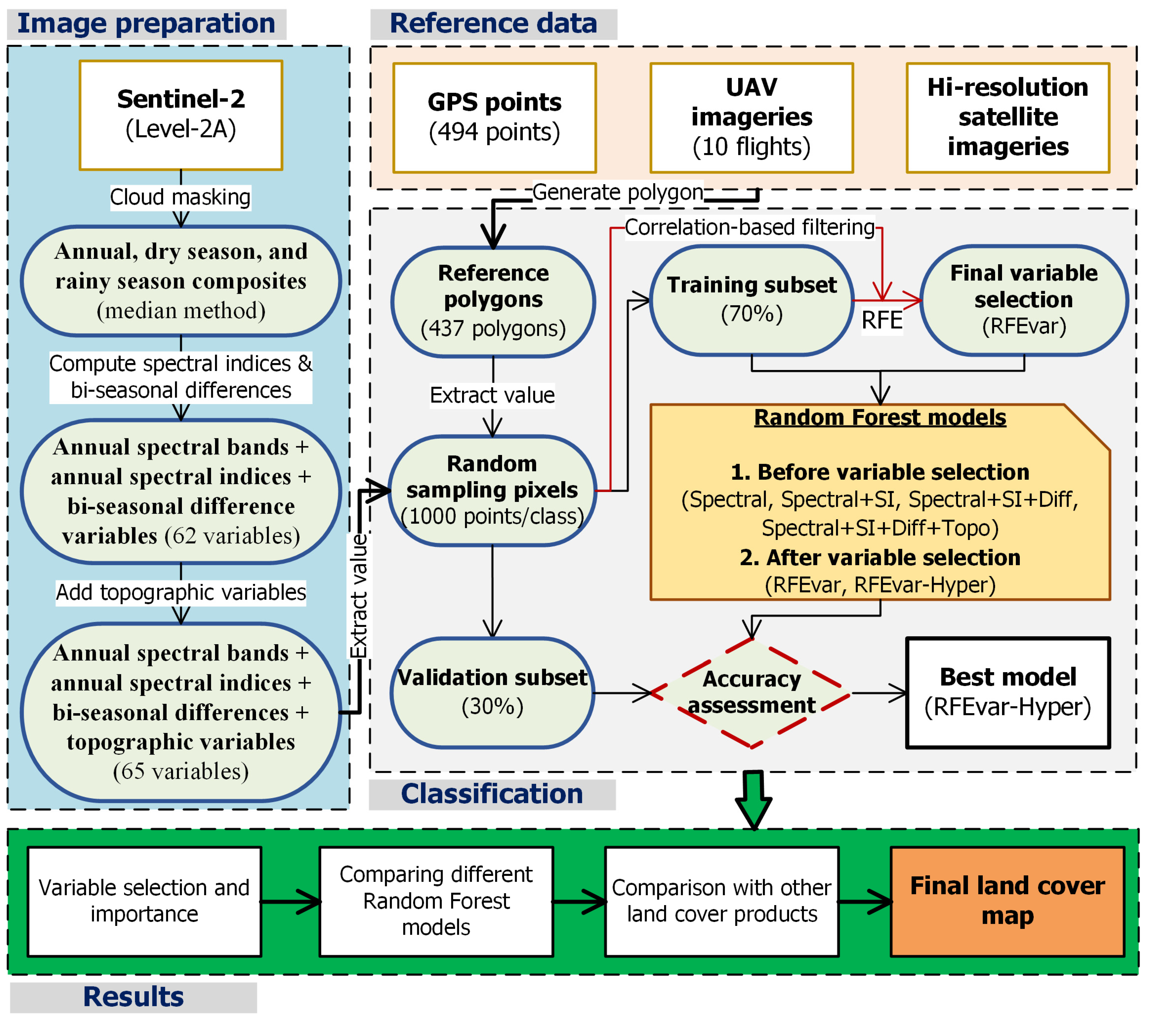
2.2.1. Overview
2.2.2. Data Sources
Sentinel-2 Dataset
Remote Sensing Indices
Bi-Seasonal Difference
Topographic Data
Reference Data of Land Cover Classes
2.2.3. Data Analyses
Random Forest Classifier and Variable Importance
Variable Selections
Comparing Different Random Forest Models
Comparison with Other Land Cover Products
3. Results
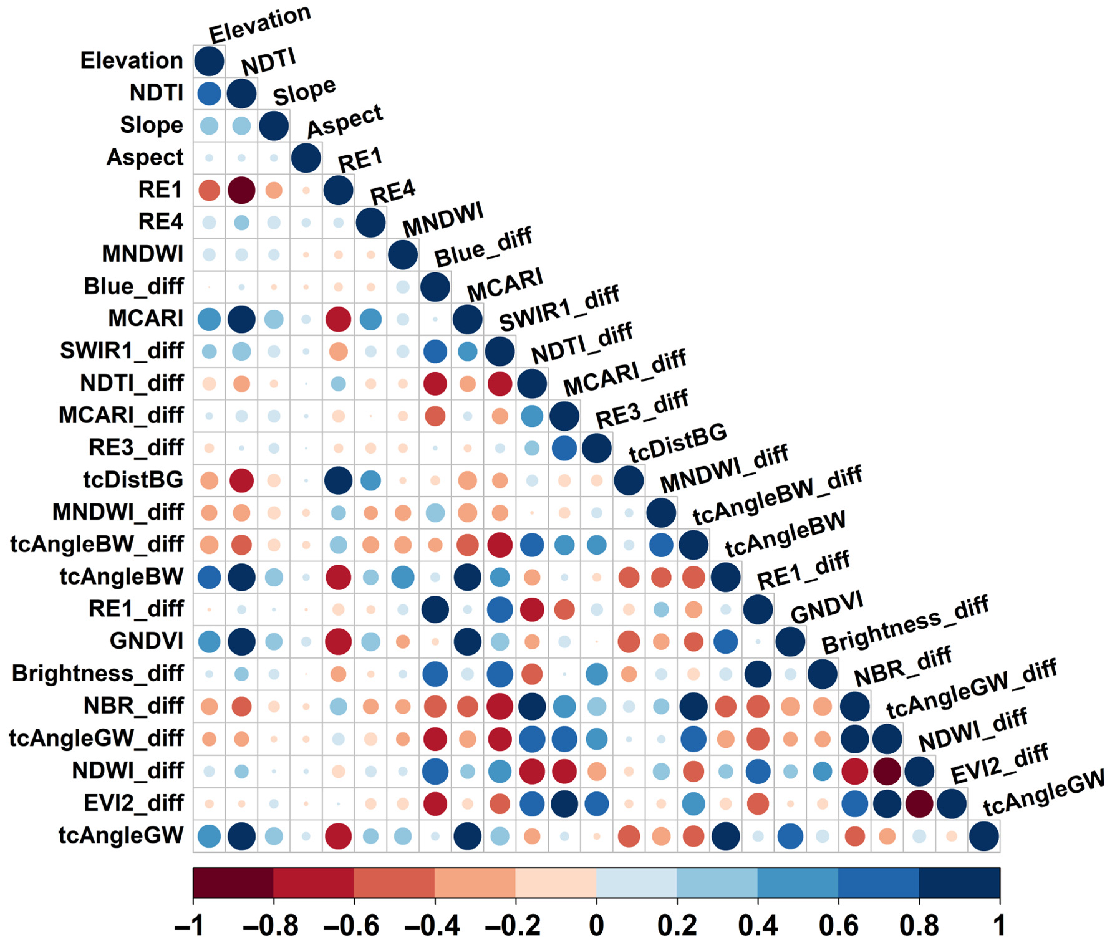
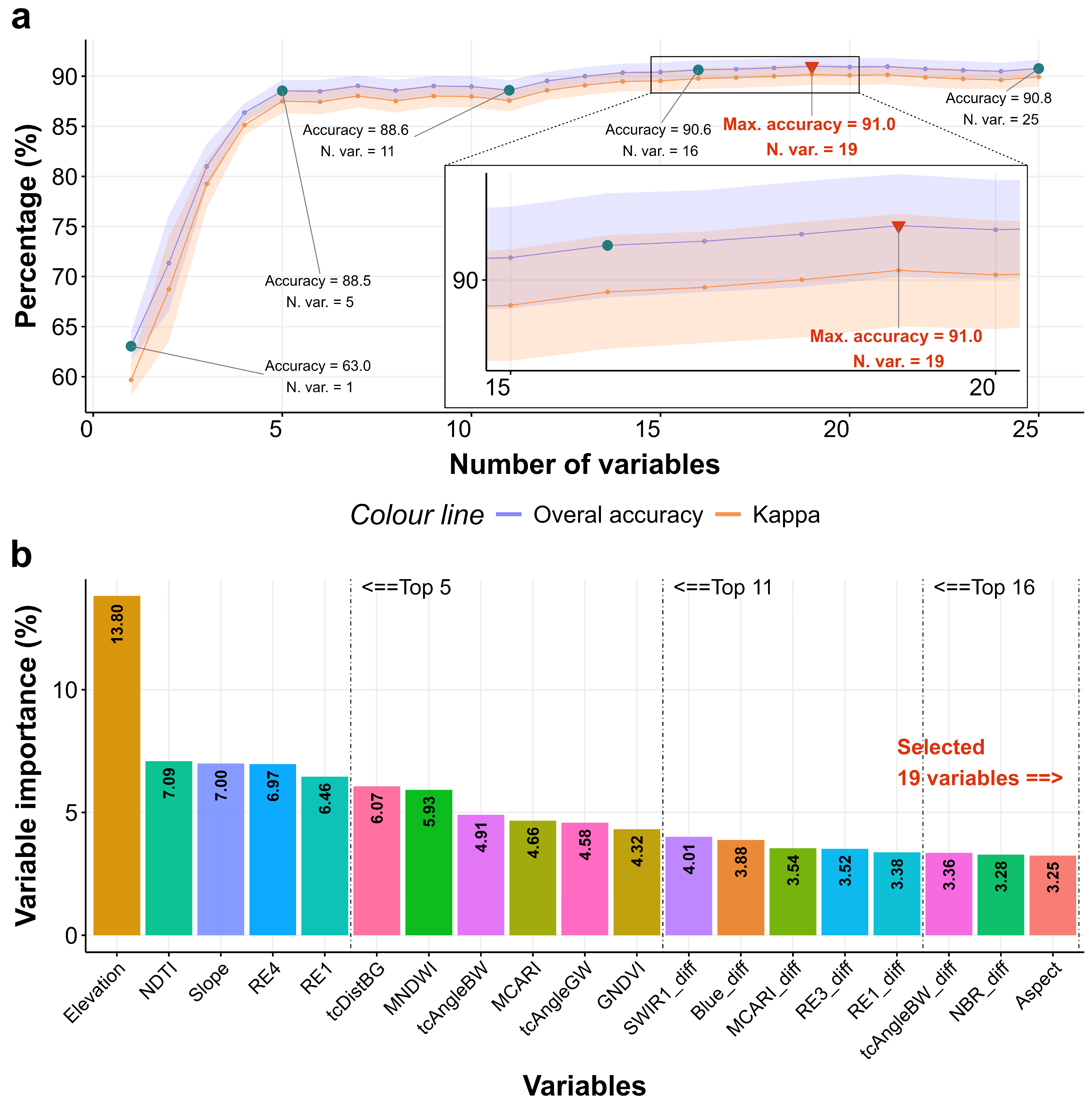
3.1. Variable Selection and Variable Importance Ranking
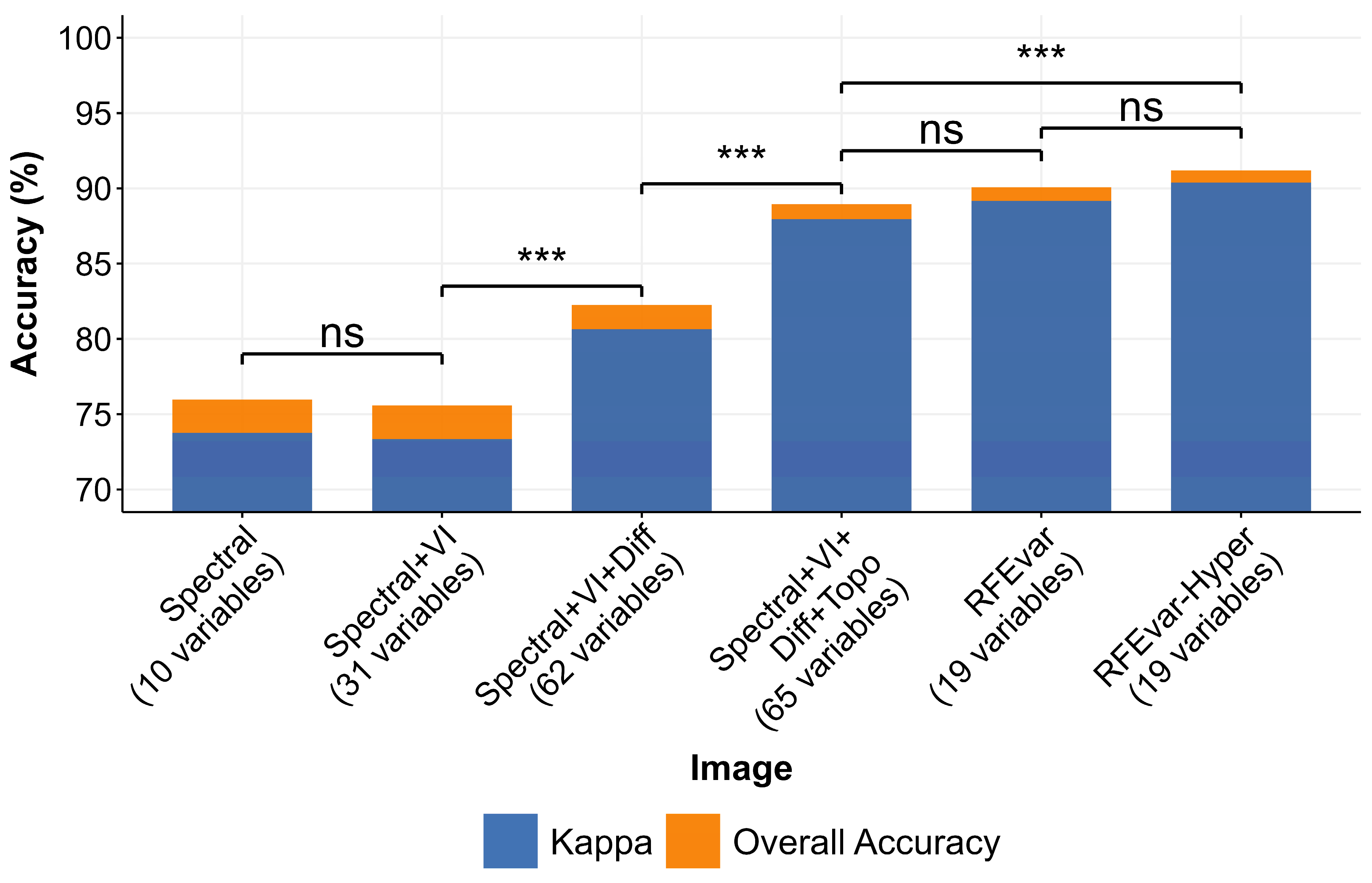
3.2. Impact of Spectral Indices, Bi-Seasonal Differences, and Topography on Accuracy in Land Cover Classification
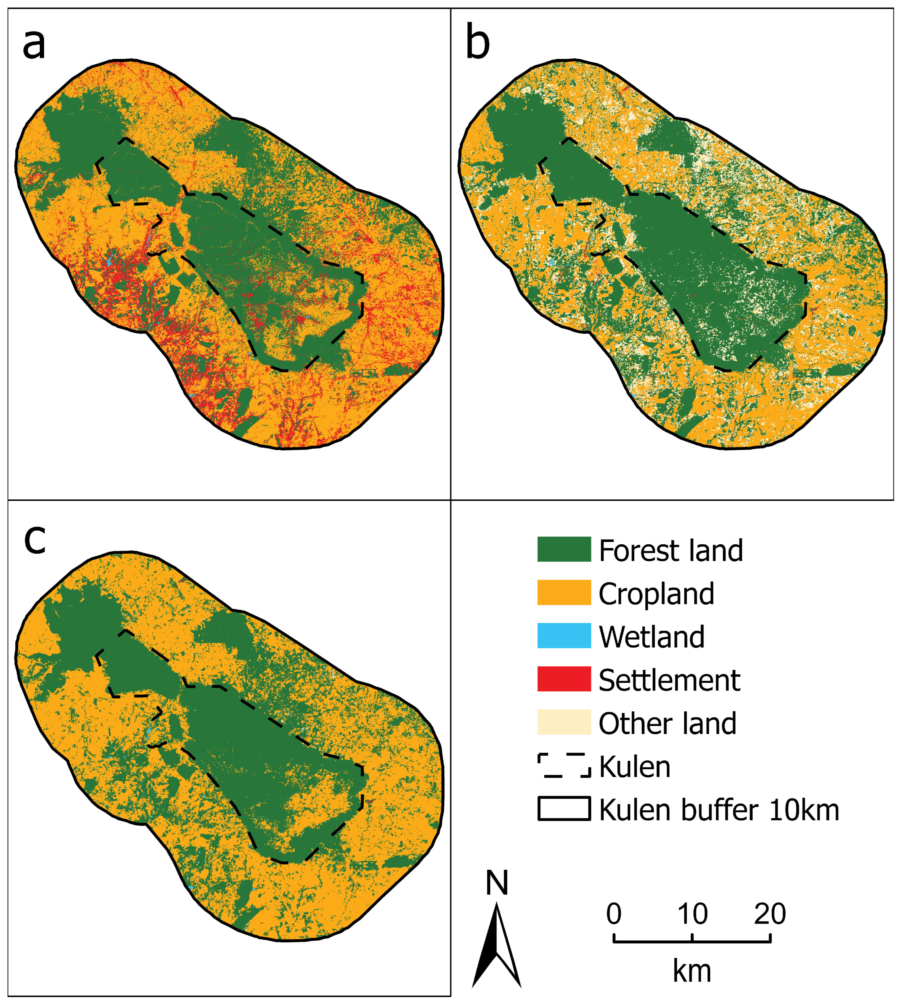
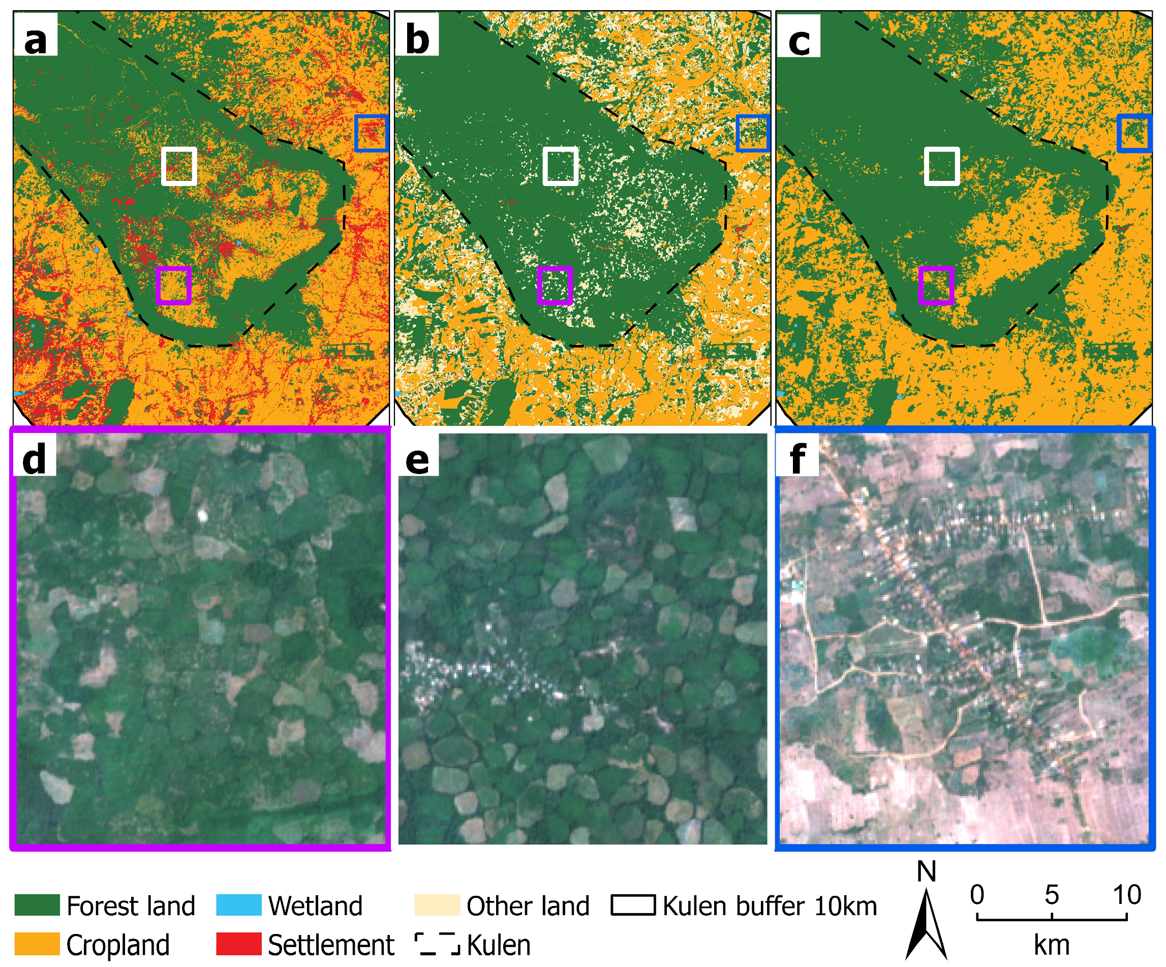
3.3. Comparison with Other Land Cover Products
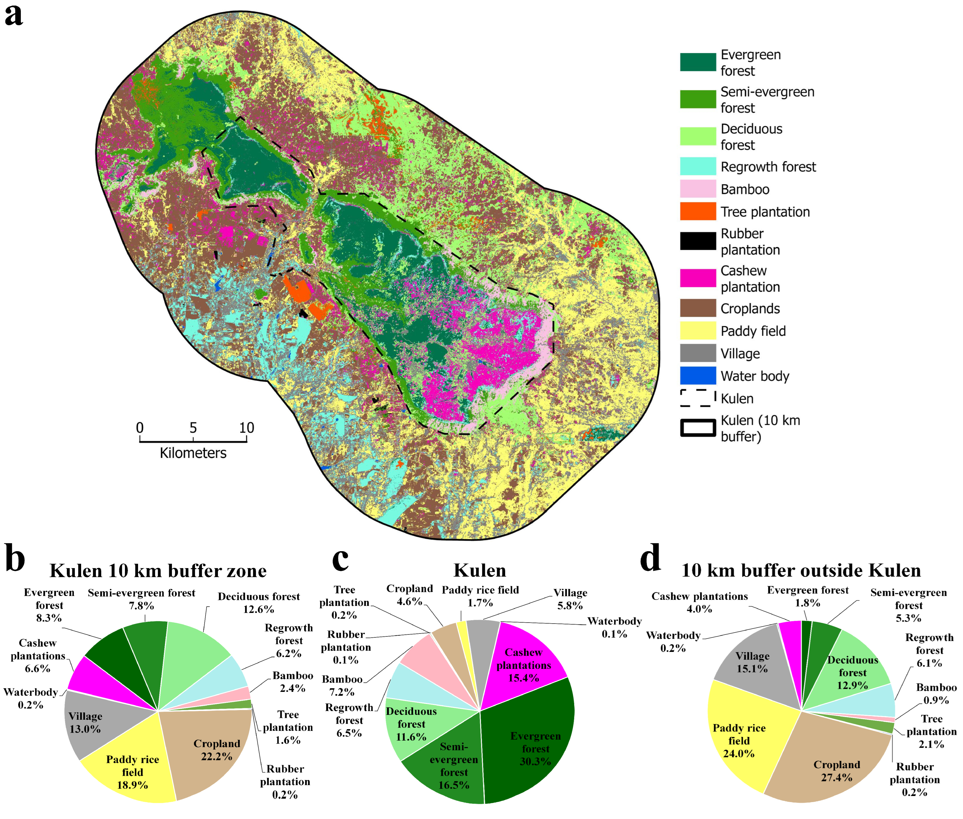
3.4. Final Land Cover Map
4. Discussions
4.1. Variable Selection and Variable Importance Ranking
4.1.1. Correlation-Based Filtering and Recursive Feature Elimination
4.1.2. Variable Importance
Impact of Topography, Tillage, SWIR, Red Edge, Water, and Vegetation Indices on Land Cover Mapping of Tropical Regions
Significance of Multi-Temporal Data in Tropical Land Cover Classification
4.2. Comparison with Other Land Cover Products
4.3. Land Cover of Kulen
5. Conclusions
Supplementary Materials
Author Contributions
Funding
Data Availability Statement
Acknowledgments
Conflicts of Interest
Abbreviations
| LC | Land cover |
| RFE | Recursive feature elimination |
| REDD+ | Reducing Emissions from Deforestation and Forest Degradation |
| RF | Random Forest |
| GEE | Google Earth Engine |
| Kulen | Phnom Kulen National Park |
| MSI | Multi-Spectral Instrument |
| NIR | Near Infrared |
| RE | Red Edge |
| SWIR | Short-Wave Infrared |
| TCT | tasseled cap transformations |
| tcAngle | tasseled cap angles |
| tcDist | tasseled cap distances |
| MNDWI | Modification Normalized Difference Water Index |
| NDWI | Normalized Difference Water Index |
| NDMI | Normalized Difference Moisture Index |
| NBR | Normalized Burn Ratio |
| NDTI | Normalized Difference Tillage Index |
| NDVI | Normalized Difference Vegetation Index |
| EVI2 | 2-band Enhanced Vegetation Index |
| GNDVI | Green Normalized Difference Vegetation Index |
| SAVI | Soil Adjusted Vegetation Index |
| NDRE | Normalized Difference Red Edge Index |
| MCARI | Modified Chlorophyll Absorption Ratio Index |
| BUI | Build-Up Index |
| SRTM | Shuttle Radar Topography Mission |
| GCP | GPS points from field observations |
| GPS | Global Positioning System |
| UAV | Uncrewed Aerial Vehicle |
| Spectral | Annual spectral bands |
| Spectral+SI | Annual spectral bands combined with spectral indices |
| Spectral+SI+Diff | Spectral+SI combined with bi-seasonal differences |
| Spectral+SI+Diff+Topo | Spectral+SI+Diff combined with topographic variables |
| RFEvar-Hyper | RFEvar with hyperparameter-tuned Random Forest |
| RFEvar | RFE-selected variables |
| OA | Overall accuracy |
| Kappa | Kappa coefficient |
| UA | User accuracy |
| PA | Producer accuracy |
| ESA | European Space Agency (ESA) WorldCover 2020 |
| KuLandCover | Our optimized LC map |
| SERVIR | SERVIR-SEA Cambodia National Land Cover 2021 |
| IPCC | Intergovernmental Panel on Climate Change |
| _diff | Suffix for bi-seasonal differences in 10 spectral bands and 21 indices. |
| NASA | National Aeronautics and Space Administration |
| ntree | numbers of decision trees |
| mtry | numbers of variables tries at each split |
| 300-tree RF | The RF model was configured with 300 trees, using the default settings of the “ee.Classifier.smileRandomForest” function in Google Earth Engine: mtry as the square root of the number of variables, minLeafPopulation as 1, bagFraction as 0.5, no limit on maxNodes, and seed as 0 |
| SD | standard deviation |
Appendix A

| No. | Land Cover Class | Description |
|---|---|---|
| 1 | Evergreen forests | Areas covered by trees maintain their leaves during the whole year. |
| 2 | Semi-evergreen forests | Contain variable percentages of evergreen and deciduous trees. |
| 3 | Deciduous forests | Comprised of dry mixed deciduous forest and dry Dipterocarp forests |
| 4 | Regrowth forests | Areas with more than 50% naturally regenerated forest with clearly visible indications of human activities (selective logging, previous agricultural land use, recovering from human-induced fire) |
| 5 | Bamboo | Areas dominated by bamboo |
| 6 | Tree plantations | Plantations of teak, eucalyptus, acacia, jatropha, and others. |
| 7 | Rubber plantations | Areas with more than 50% rubber plantation. |
| 8 | Croplands | Arable and tillage land, and agro-forestry systems where tree cover falls below the thresholds used for the forest land category. Examples of cropland include cassava and mango plantations. |
| 9 | Paddy rice fields | Flooded parcels of arable land used for growing semi-aquatic rice. |
| 10 | Villages | The patch of land with houses and gardens surrounding the house. |
| 11 | Water bodies | Area of fresh and seawater |
| 12 | Cashew plantations | This area is primarily dominated by cashew trees, ranging from small household-scale plantations to larger commercial plantations. |
| Product | Resolution | Data | Coverage | Classes | Reference |
|---|---|---|---|---|---|
| ESA WorldCover 10 m 2020 v100 | 10 m | 2020 | Global | Tree cover, shrubland, mangroves, cropland, bare/sparse vegetation, permanent water bodies, herbaceous wetland, built-up, grassland, snow and ice, moss and lichen. | [90] |
| SERVIR-SEA Cambodia National Land Cover | 30 m | 2021 | Cambodia | Mangrove, shrub, evergreen, deciduous, flooded forest, semi-evergreen, other plantation, rice, cropland, rubber, water, wetland, built-up area, village, grass, others. | [89] |
| IPCC Land Covers [91] | Original LC Classes | ||
|---|---|---|---|
| ESA [127] | SERVIR [89] | Our Reference Polygons and LC Product | |
| Forest land | Tree cover, shrubland | Evergreen, deciduous, semi-evergreen, flooded forest, shrub | Evergreen forest, semi-evergreen forest, deciduous forest, regrowth forest, bamboo, tree plantation |
| Cropland | Cropland, bare/sparse vegetation | Other plantations, rice, cropland, rubber | Rubber plantation, cropland, paddy field, cashew |
| Wetland | Permanent water bodies, herbaceous wetland | Water, wetland | Water |
| Settlement | Built-up | Built-up area, village | Village |
| Other land | Grassland | Grass, others | - |

References
- Brandon, K. Ecosystem services from tropical forests: Review of current science. Cent. Glob. Dev. Work. Pap. 2014, 7, 380. [Google Scholar] [CrossRef]
- Leemans, R.; De Groot, R.S. Millennium Ecosystem Assessment: Ecosystems and Human Well-Being: A Framework for Assessment; CIFOR: Bogor, Indonesia, 2003. [Google Scholar]
- Artaxo, P.; Hansson, H.C.; Machado, L.A.T.; Rizzo, L.V. Tropical forests are crucial in regulating the climate on Earth. PLoS Clim. 2022, 1, e0000054. [Google Scholar] [CrossRef]
- Davis, K.F.; Koo, H.I.; Dell’Angelo, J.; D’Odorico, P.; Estes, L.; Kehoe, L.J.; Kharratzadeh, M.; Kuemmerle, T.; Machava, D.; Pais, A.d.J.R.; et al. Tropical forest loss enhanced by large-scale land acquisitions. Nat. Geosci. 2020, 13, 482–488. [Google Scholar] [CrossRef]
- Lamarre, G.P.A.; Fayle, T.M.; Segar, S.T.; Laird-Hopkins, B.C.; Nakamura, A.; Souto-Vilarós, D.; Watanabe, S.; Basset, Y. Chapter Eight—Monitoring tropical insects in the 21st century. In Advances in Ecological Research; Dumbrell, A.J., Turner, E.C., Fayle, T.M., Eds.; Academic Press: Cambridge, MA, USA, 2020; Volume 62, pp. 295–330. [Google Scholar]
- Pauly, M.; Crosse, W.; Tosteson, J. High deforestation trajectories in Cambodia slowly transformed through economic land concession restrictions and strategic execution of REDD+ protected areas. Sci. Rep. 2022, 12, 17102. [Google Scholar] [CrossRef]
- Kobayashi, S. Landscape rehabilitation of degraded tropical forest ecosystems: Case study of the CIFOR/Japan project in Indonesia and Peru. For. Ecol. Manag. 2004, 201, 13–22. [Google Scholar] [CrossRef]
- Agrawal, A.; Nepstad, D.; Chhatre, A. Reducing Emissions from Deforestation and Forest Degradation. Annu. Rev. Environ. Resour. 2011, 36, 373–396. [Google Scholar] [CrossRef]
- Zekeng, J.C.; Sebego, R.; Mphinyane, W.N.; Mpalo, M.; Nayak, D.; Fobane, J.L.; Onana, J.M.; Funwi, F.P.; Mbolo, M.M.A. Land use and land cover changes in Doume Communal Forest in eastern Cameroon: Implications for conservation and sustainable management. Model. Earth Syst. Environ. 2019, 5, 1801–1814. [Google Scholar] [CrossRef]
- Wang, C.; Yu, M.; Gao, Q. Continued Reforestation and Urban Expansion in the New Century of a Tropical Island in the Caribbean. Remote Sens. 2017, 9, 731. [Google Scholar] [CrossRef]
- Tsai, Y.H.; Stow, D.; Chen, H.L.; Lewison, R.; An, L.; Shi, L. Mapping Vegetation and Land Use Types in Fanjingshan National Nature Reserve Using Google Earth Engine. Remote Sens. 2018, 10, 927. [Google Scholar] [CrossRef]
- Ferrer Velasco, R.; Lippe, M.; Tamayo, F.; Mfuni, T.; Sales-Come, R.; Mangabat, C.; Schneider, T.; Günter, S. Towards accurate mapping of forest in tropical landscapes: A comparison of datasets on how forest transition matters. Remote Sens. Environ. 2022, 274, 112997. [Google Scholar] [CrossRef]
- Nguyen, H.T.; Doan, T.M.; Tomppo, E.; McRoberts, R.E. Land Use/Land Cover Mapping Using Multitemporal Sentinel-2 Imagery and Four Classification Methods—A Case Study from Dak Nong, Vietnam. Remote Sens. 2020, 12, 1367. [Google Scholar] [CrossRef]
- Eggen, M.; Ozdogan, M.; Zaitchik, B.F.; Simane, B. Land Cover Classification in Complex and Fragmented Agricultural Landscapes of the Ethiopian Highlands. Remote Sens. 2016, 8, 1020. [Google Scholar] [CrossRef]
- Pizarro, S.E.; Pricope, N.G.; Vargas-Machuca, D.; Huanca, O.; Ñaupari, J. Mapping Land Cover Types for Highland Andean Ecosystems in Peru Using Google Earth Engine. Remote Sens. 2022, 14, 1562. [Google Scholar] [CrossRef]
- Salinas-Melgoza, M.A.; Skutsch, M.; Lovett, J.C. Predicting aboveground forest biomass with topographic variables in human-impacted tropical dry forest landscapes. Ecosphere 2018, 9, e02063. [Google Scholar] [CrossRef]
- Gregorutti, B.; Michel, B.; Saint-Pierre, P. Correlation and variable importance in random forests. Stat. Comput. 2017, 27, 659–678. [Google Scholar] [CrossRef]
- Hamad, Z.O. Review Of Feature Selection Methods Using Optimization Algorithm (Review Paper For Optimization Algorithm). Polytech. J. 2023, 12, 24. [Google Scholar] [CrossRef]
- Jović, A.; Brkić, K.; Bogunović, N. A review of feature selection methods with applications. In Proceedings of the 2015 38th International Convention on Information and Communication Technology, Electronics and Microelectronics (MIPRO), Opatija, Croatia, 25–29 May 2015; pp. 1200–1205. [Google Scholar]
- Schulz, D.; Yin, H.; Tischbein, B.; Verleysdonk, S.; Adamou, R.; Kumar, N. Land use mapping using Sentinel-1 and Sentinel-2 time series in a heterogeneous landscape in Niger, Sahel. ISPRS J. Photogramm. Remote Sens. 2021, 178, 97–111. [Google Scholar] [CrossRef]
- Demarchi, L.; Kania, A.; Ciężkowski, W.; Piórkowski, H.; Oświecimska-Piasko, Z.; Chormański, J. Recursive Feature Elimination and Random Forest Classification of Natura 2000 Grasslands in Lowland River Valleys of Poland Based on Airborne Hyperspectral and LiDAR Data Fusion. Remote Sens. 2020, 12, 1842. [Google Scholar] [CrossRef]
- Ramezan, C.A. Transferability of Recursive Feature Elimination (RFE)-Derived Feature Sets for Support Vector Machine Land Cover Classification. Remote Sens. 2022, 14, 6218. [Google Scholar] [CrossRef]
- Ma, Z.; Li, W.; Warner, T.A.; He, C.; Wang, X.; Zhang, Y.; Guo, C.; Cheng, T.; Zhu, Y.; Cao, W.; et al. A framework combined stacking ensemble algorithm to classify crop in complex agricultural landscape of high altitude regions with Gaofen-6 imagery and elevation data. Int. J. Appl. Earth Obs. Geoinf. 2023, 122, 103386. [Google Scholar] [CrossRef]
- Cánovas-García, F.; Alonso-Sarría, F. Optimal Combination of Classification Algorithms and Feature Ranking Methods for Object-Based Classification of Submeter Resolution Z/I-Imaging DMC Imagery. Remote Sens. 2015, 7, 4651–4677. [Google Scholar] [CrossRef]
- Georganos, S.; Grippa, T.; Vanhuysse, S.; Lennert, M.; Shimoni, M.; Kalogirou, S.; Wolff, E. Less is more: Optimizing classification performance through feature selection in a very-high-resolution remote sensing object-based urban application. GIScience Remote Sens. 2018, 55, 221–242. [Google Scholar] [CrossRef]
- Xu, S.; Xiao, W.; Ruan, L.; Chen, W.; Du, J. Assessment of ensemble learning for object-based land cover mapping using multi-temporal Sentinel-1/2 images. Geocarto Int. 2023, 38, 2195832. [Google Scholar] [CrossRef]
- Manandhar, R.; Odeh, I.O.A.; Ancev, T. Improving the Accuracy of Land Use and Land Cover Classification of Landsat Data Using Post-Classification Enhancement. Remote Sens. 2009, 1, 330–344. [Google Scholar] [CrossRef]
- Nguyen, T.T.H. Forestry Remote Sensing: Multi-Source Data in Natural Evergreen Forest Inventory in the Central Highlands of Vietnam; LAP LAMBERT Academic Publishing: Saarbrücken, Germany, 2011. [Google Scholar]
- Heydari, S.S.; Mountrakis, G. Effect of classifier selection, reference sample size, reference class distribution and scene heterogeneity in per-pixel classification accuracy using 26 Landsat sites. Remote Sens. Environ. 2018, 204, 648–658. [Google Scholar] [CrossRef]
- Breiman, L. Random Forests. Mach. Learn. 2001, 45, 5–32. [Google Scholar] [CrossRef]
- Georganos, S.; Grippa, T.; Niang Gadiaga, A.; Linard, C.; Lennert, M.; Vanhuysse, S.; Mboga, N.; Wolff, E.; Kalogirou, S. Geographical random forests: A spatial extension of the random forest algorithm to address spatial heterogeneity in remote sensing and population modelling. Geocarto Int. 2019, 36, 121–136. [Google Scholar] [CrossRef]
- Belgiu, M.; Drăguţ, L. Random forest in remote sensing: A review of applications and future directions. ISPRS J. Photogramm. Remote Sens. 2016, 114, 24–31. [Google Scholar] [CrossRef]
- Pelletier, C.; Valero, S.; Inglada, J.; Champion, N.; Dedieu, G. Assessing the robustness of Random Forests to map land cover with high resolution satellite image time series over large areas. Remote Sens. Environ. 2016, 187, 156–168. [Google Scholar] [CrossRef]
- Tieng, T.; Sharma, S.; MacKenzie, R.A.; Venkattappa, M.; Sasaki, N.K.; Collin, A. Mapping mangrove forest cover using Landsat-8 imagery, Sentinel-2, Very High Resolution Images and Google Earth Engine algorithm for entire Cambodia. IOP Conf. Ser. Earth Environ. Sci. 2019, 266, 012010. [Google Scholar] [CrossRef]
- Nguyen, H.T.T.; Doan, T.M.; Radeloff, V. Applying random forest classification to map land use/land cover using Landsat 8 OLI. Int. Arch. Photogramm. Remote Sens. Spat. Inf. Sci. 2018, 42, 363–367. [Google Scholar] [CrossRef]
- Ha, T.V.; Tuohy, M.; Irwin, M.; Tuan, P.V. Monitoring and mapping rural urbanization and land use changes using Landsat data in the northeast subtropical region of Vietnam. Egypt. J. Remote Sens. Space Sci. 2020, 23, 11–19. [Google Scholar] [CrossRef]
- Gorelick, N.; Hancher, M.; Dixon, M.; Ilyushchenko, S.; Thau, D.; Moore, R. Google Earth Engine: Planetary-scale geospatial analysis for everyone. Remote Sens. Environ. 2017, 202, 18–27. [Google Scholar] [CrossRef]
- Amani, M.; Ghorbanian, A.; Ahmadi, S.A.; Kakooei, M.; Moghimi, A.; Mirmazloumi, S.M.; Moghaddam, S.H.A.; Mahdavi, S.; Ghahremanloo, M.; Parsian, S.; et al. Google Earth Engine Cloud Computing Platform for Remote Sensing Big Data Applications: A Comprehensive Review. IEEE J. Sel. Top. Appl. Earth Obs. Remote Sens. 2020, 13, 5326–5350. [Google Scholar] [CrossRef]
- Geissler, P.; Hartmann, T.; Ihlow, F.; Neang, T.; Seng, R.; Wagner, P.; Bohme, W. Herpetofauna of the Phnom Kulen. Cambodian J. Nat. Hist. 2019, 40, 780. [Google Scholar]
- Sovann, C.; Tagesson, T.; Vestin, P.; Sakhoeun, S.; Kim, S.; Kok, S.; Olin, S. Characteristics of ecosystems under various anthropogenic impacts in a tropical forest region of Southeast Asia. EGUsphere 2025, 2025, 3784. [Google Scholar] [CrossRef]
- Somaly, O.; Sasaki, N.; Kimchhin, S.; Tsusaka, T.W.; Shrestha, S.; Malyne, N. Impact of Forest Cover Change in Phnom Kulen National Park on Downstream Local Livelihoods along Siem Reap River, Cambodia. Int. J. Environ. Rural Dev. 2020, 11, 93–99. [Google Scholar] [CrossRef]
- Hang, P.; Ishwaran, N.; Hong, T.; Delanghe, P. From Conservation to Sustainable Development—A Case Study of Angkor World Heritage Site, Cambodia. J. Environ. Sci. Eng. A 2016, 5, 141–155. [Google Scholar] [CrossRef]
- Provincial Department of Planning Siem Reap. Commune Socio-Economic Situation; Provincial Department of Planning Siem Reap: Siem Reap, Cambodia, 2024.
- Magliocca, N.R.; Khuc, Q.V.; de Bremond, A.; Ellicott, E.A. Direct and indirect land-use change caused by large-scale land acquisitions in Cambodia. Environ. Res. Lett. 2020, 15, 024010. [Google Scholar] [CrossRef]
- Motzke, I.; Wanger, T.C.; Zanre, E.; Tscharntke, T.; Barkmann, J. Socio-economic context of forest biodiversity use along a town-forest gradient in Cambodia. Raffles Bull. Zool. 2012, 30, 37–53. [Google Scholar]
- Chim, K.; Tunnicliffe, J.; Shamseldin, A.; Ota, T. Land Use Change Detection and Prediction in Upper Siem Reap River, Cambodia. Hydrol.-Basel 2019, 6, 64. [Google Scholar] [CrossRef]
- Singh, M.; Evans, D.; Chevance, J.-B.; Tan, B.S.; Wiggins, N.; Kong, L.; Sakhoeun, S. Evaluating remote sensing datasets and machine learning algorithms for mapping plantations and successional forests in Phnom Kulen National Park of Cambodia. PeerJ 2019, 7, e7841. [Google Scholar] [CrossRef] [PubMed]
- Drusch, M.; Del Bello, U.; Carlier, S.; Colin, O.; Fernandez, V.; Gascon, F.; Hoersch, B.; Isola, C.; Laberinti, P.; Martimort, P.; et al. Sentinel-2: ESA’s Optical High-Resolution Mission for GMES Operational Services. Remote Sens. Environ. 2012, 120, 25–36. [Google Scholar] [CrossRef]
- Gorroño, J.; Banks, A.C.; Fox, N.P.; Underwood, C. Radiometric inter-sensor cross-calibration uncertainty using a traceable high accuracy reference hyperspectral imager. ISPRS J. Photogramm. Remote Sens. 2017, 130, 393–417. [Google Scholar] [CrossRef]
- Müller-Wilm, U.; Devignot, O.; Pessiot, L. S2 MPC Sen2Cor Configuration and User Manual; EASE: San Francisco, CA, USA, 2017. [Google Scholar]
- Hosseiny, B.; Abdi, A.M.; Jamali, S. Urban land use and land cover classification with interpretable machine learning—A case study using Sentinel-2 and auxiliary data. Remote Sens. Appl. Soc. Environ. 2022, 28, 100843. [Google Scholar] [CrossRef]
- Pour, A.B.; Ranjbar, H.; Sekandari, M.; Abd El-Wahed, M.; Hossain, M.S.; Hashim, M.; Yousefi, M.; Zoheir, B.; Wambo, J.D.T.; Muslim, A.M. 2-Remote sensing for mineral exploration. In Geospatial Analysis Applied to Mineral Exploration; Pour, A.B., Parsa, M., Eldosouky, A.M., Eds.; Elsevier: Amsterdam, The Netherlands, 2023; pp. 17–149. [Google Scholar]
- Shi, T.; Xu, H. Derivation of Tasseled Cap Transformation Coefficients for Sentinel-2 MSI At-Sensor Reflectance Data. IEEE J. Sel. Top. Appl. Earth Obs. Remote Sens. 2019, 12, 4038–4048. [Google Scholar] [CrossRef]
- Powell, S.L.; Cohen, W.B.; Healey, S.P.; Kennedy, R.E.; Moisen, G.G.; Pierce, K.B.; Ohmann, J.L. Quantification of live aboveground forest biomass dynamics with Landsat time-series and field inventory data: A comparison of empirical modeling approaches. Remote Sens. Environ. 2010, 114, 1053–1068. [Google Scholar] [CrossRef]
- Saah, D.; Tenneson, K.; Poortinga, A.; Nguyen, Q.; Chishtie, F.; Aung, K.S.; Markert, K.N.; Clinton, N.; Anderson, E.R.; Cutter, P.; et al. Primitives as building blocks for constructing land cover maps. Int. J. Appl. Earth Obs. Geoinf. 2020, 85, 101979. [Google Scholar] [CrossRef]
- Xu, H. Modification of normalised difference water index (NDWI) to enhance open water features in remotely sensed imagery. Int. J. Remote Sens. 2006, 27, 3025–3033. [Google Scholar] [CrossRef]
- McFeeters, S.K. The use of the Normalized Difference Water Index (NDWI) in the delineation of open water features. Int. J. Remote Sens. 1996, 17, 1425–1432. [Google Scholar] [CrossRef]
- Gao, B.-C. NDWI—A normalized difference water index for remote sensing of vegetation liquid water from space. Remote Sens. Environ. 1996, 58, 257–266. [Google Scholar] [CrossRef]
- García, M.J.L.; Caselles, V. Mapping burns and natural reforestation using thematic Mapper data. Geocarto Int. 1991, 6, 31–37. [Google Scholar] [CrossRef]
- Van Deventer, A.P.; Ward, A.D.; Gowda, P.M.; Lyon, J.G. Using thematic mapper data to identify contrasting soil plains and tillage practices. Photogramm. Eng. Remote Sens. 1997, 63, 87–93. [Google Scholar]
- Rouse, J.W.; Haas, R.H.; Schell, J.A.; Deering, D.W. Monitoring Vegetation Systems in the Great Plains with ERTS; NASA: Washington, DC, UAS, 1973. [Google Scholar]
- Jiang, Z.; Huete, A.R.; Didan, K.; Miura, T. Development of a two-band enhanced vegetation index without a blue band. Remote Sens. Environ. 2008, 112, 3833–3845. [Google Scholar] [CrossRef]
- Huang, X.; Xiao, J.; Ma, M. Evaluating the Performance of Satellite-Derived Vegetation Indices for Estimating Gross Primary Productivity Using FLUXNET Observations across the Globe. Remote Sens. 2019, 11, 1823. [Google Scholar] [CrossRef]
- Gitelson, A.A.; Kaufman, Y.J.; Merzlyak, M.N. Use of a green channel in remote sensing of global vegetation from EOS-MODIS. Remote Sens. Environ. 1996, 58, 289–298. [Google Scholar] [CrossRef]
- Huete, A.R. A soil-adjusted vegetation index (SAVI). Remote Sens. Environ. 1988, 25, 295–309. [Google Scholar] [CrossRef]
- Barnes, E.M.; Clarke, T.R.; Richards, S.E.; Colaizzi, P.D.; Haberland, J.; Kostrzewski, M.; Waller, P.; Choi, C.; Riley, E.; Thompson, T. Coincident detection of crop water stress, nitrogen status and canopy density using ground based multispectral data. In Proceedings of the Fifth International Conference on Precision Agriculture, Bloomington, MN, USA, 16 July 2000. [Google Scholar]
- Daughtry, C.S.T.; Walthall, C.L.; Kim, M.S.; de Colstoun, E.B.; McMurtrey, J.E. Estimating Corn Leaf Chlorophyll Concentration from Leaf and Canopy Reflectance. Remote Sens. Environ. 2000, 74, 229–239. [Google Scholar] [CrossRef]
- Zhang, H.; Li, J.; Liu, Q.; Lin, S.; Huete, A.; Liu, L.; Croft, H.; Clevers, J.G.P.W.; Zeng, Y.; Wang, X.; et al. A novel red-edge spectral index for retrieving the leaf chlorophyll content. Methods Ecol. Evol. 2022, 13, 2771–2787. [Google Scholar] [CrossRef]
- He, C.; Shi, P.; Xie, D.; Zhao, Y. Improving the normalized difference built-up index to map urban built-up areas using a semiautomatic segmentation approach. Remote Sens. Lett. 2010, 1, 213–221. [Google Scholar] [CrossRef]
- Farr, T.G.; Rosen, P.A.; Caro, E.; Crippen, R.; Duren, R.; Hensley, S.; Kobrick, M.; Paller, M.; Rodriguez, E.; Roth, L.; et al. The Shuttle Radar Topography Mission. Rev. Geophys. 2007, 45, 2. [Google Scholar] [CrossRef]
- Ministry of Environment (Cambodia). Cambodia Forest Cover 2018; Ministry of Environment (Cambodia): Phnom Penh, Cambodia, 2020.
- Planet Team. Planet Application Program Interface: In Space for Life on Earth; NASA: San Francisco, CA, USA, 2017. [Google Scholar]
- Pedergnana, M.; Marpu, P.R.; Mura, M.D.; Benediktsson, J.A.; Bruzzone, L. Classification of Remote Sensing Optical and LiDAR Data Using Extended Attribute Profiles. IEEE J. Sel. Top. Signal Process. 2012, 6, 856–865. [Google Scholar] [CrossRef]
- Lu, D.; Weng, Q. A survey of image classification methods and techniques for improving classification performance. Int. J. Remote Sens. 2007, 28, 823–870. [Google Scholar] [CrossRef]
- Zhang, F.; Yang, X. Improving land cover classification in an urbanized coastal area by random forests: The role of variable selection. Remote Sens. Environ. 2020, 251, 112105. [Google Scholar] [CrossRef]
- Vizzari, M.; Lesti, G.; Acharki, S. Crop classification in Google Earth Engine: Leveraging Sentinel-1, Sentinel-2, European CAP data, and object-based machine-learning approaches. Geo-Spat. Inf. Sci. 2024, 27, 1–16. [Google Scholar] [CrossRef]
- Badda, H.; Cherif, E.K.; Boulaassal, H.; Wahbi, M.; Yazidi Alaoui, O.; Maatouk, M.; Bernardino, A.; Coren, F.; El Kharki, O. Improving the Accuracy of Random Forest Classifier for Identifying Burned Areas in the Tangier-Tetouan-Al Hoceima Region Using Google Earth Engine. Remote Sens. 2023, 15, 4226. [Google Scholar] [CrossRef]
- Behnamian, A.; Millard, K.; Banks, S.N.; White, L.; Richardson, M.; Pasher, J. A Systematic Approach for Variable Selection With Random Forests: Achieving Stable Variable Importance Values. IEEE Geosci. Remote Sens. Lett. 2017, 14, 1988–1992. [Google Scholar] [CrossRef]
- Kuhn, M. Building Predictive Models in R Using the caret Package. J. Stat. Softw. 2008, 28, 1–26. [Google Scholar] [CrossRef]
- Shih, H.-C.; Stow, D.A.; Tsai, Y.H. Guidance on and comparison of machine learning classifiers for Landsat-based land cover and land use mapping. Int. J. Remote Sens. 2019, 40, 1248–1274. [Google Scholar] [CrossRef]
- Sun, J.; Ongsomwang, S. Optimal parameters of random forest for land cover classification with suitable data type and dataset on Google Earth Engine. Front. Earth Sci. 2023, 11, 1188093. [Google Scholar] [CrossRef]
- Congalton, R.G.; Green, K. Assessing the Accuracy of Remotely Sensed Data: Principles and Practices; CRC Press: Boca Raton, FL, USA, 2019. [Google Scholar]
- Foody, G.M. Explaining the unsuitability of the kappa coefficient in the assessment and comparison of the accuracy of thematic maps obtained by image classification. Remote Sens. Environ. 2020, 239, 111630. [Google Scholar] [CrossRef]
- Olofsson, P.; Foody, G.M.; Herold, M.; Stehman, S.V.; Woodcock, C.E.; Wulder, M.A. Good practices for estimating area and assessing accuracy of land change. Remote Sens. Environ. 2014, 148, 42–57. [Google Scholar] [CrossRef]
- Congalton, R.G.; Oderwald, R.G.; Mead, R.A. Assessing Landsat classification accuracy using discrete multivariate analysis statistical techniques. Photogramm. Eng. Remote Sens. 1983, 49, 1671–1678. [Google Scholar]
- Anderson, J.R.; Hardy, E.E.; Roach, J.T.; Witmer, R.E. A Land Use and Land Cover Classification System for Use with Remote Sensor Data; U.S. Government Printing Office: Washington, DC, USA, 1976; p. 964.
- Foody, G.M. Status of land cover classification accuracy assessment. Remote Sens. Environ. 2002, 80, 185–201. [Google Scholar] [CrossRef]
- Xia, T.; He, Z.; Cai, Z.; Wang, C.; Wang, W.; Wang, J.; Hu, Q.; Song, Q. Exploring the potential of Chinese GF-6 images for crop mapping in regions with complex agricultural landscapes. Int. J. Appl. Earth Obs. Geoinf. 2022, 107, 102702. [Google Scholar] [CrossRef]
- SERVIR-SEA. Cambodia Biophysical Monitoring and Evaluation Dashboard. Available online: https://servir.adpc.net/tools/biophysical-me-dashboard (accessed on 8 November 2024).
- Zanaga, D.; Van De Kerchove, R.; De Keersmaecker, W.; Souverijns, N.; Brockmann, C.; Quast, R.; Wevers, J.; Grosu, A.; Paccini, A.; Vergnaud, S.; et al. ESA WorldCover 10 m 2020 v100; Zenodo: Genève, Switzerland, 2021. [Google Scholar] [CrossRef]
- IPCC. 2006 IPCC Guidelines for National Greenhouse Gas Inventorie; Eggleston, H.S., Buendia, L., Miwa, K., Ngara, T., Tanabe, K., Eds.; IGES: Kanagawa, Japan, 2006. [Google Scholar]
- Jin, Z.; Azzari, G.; You, C.; Di Tommaso, S.; Aston, S.; Burke, M.; Lobell, D.B. Smallholder maize area and yield mapping at national scales with Google Earth Engine. Remote Sens. Environ. 2019, 228, 115–128. [Google Scholar] [CrossRef]
- Kasraei, B.; Schmidt, M.G.; Zhang, J.; Bulmer, C.E.; Filatow, D.S.; Arbor, A.; Pennell, T.; Heung, B. A framework for optimizing environmental covariates to support model interpretability in digital soil mapping. Geoderma 2024, 445, 116873. [Google Scholar] [CrossRef]
- Liu, H.; An, H. Preliminary tests on the performance of MLC-RFE and SVM-RFE in Lansat-8 image classification. Arab. J. Geosci. 2020, 13, 130. [Google Scholar] [CrossRef]
- Wei, X.; Zhang, W.; Zhang, Z.; Huang, H.; Meng, L. Urban land use land cover classification based on GF-6 satellite imagery and multi-feature optimization. Geocarto Int. 2023, 38, 2236579. [Google Scholar] [CrossRef]
- Xing, H.; Niu, J.; Feng, Y.; Hou, D.; Wang, Y.; Wang, Z. A coastal wetlands mapping approach of Yellow River Delta with a hierarchical classification and optimal feature selection framework. CATENA 2023, 223, 106897. [Google Scholar] [CrossRef]
- Qian, H.; Bao, N.; Meng, D.; Zhou, B.; Lei, H.; Li, H. Mapping and classification of Liao River Delta coastal wetland based on time series and multi-source GaoFen images using stacking ensemble model. Ecol. Inform. 2024, 80, 102488. [Google Scholar] [CrossRef]
- Grabska, E.; Frantz, D.; Ostapowicz, K. Evaluation of machine learning algorithms for forest stand species mapping using Sentinel-2 imagery and environmental data in the Polish Carpathians. Remote Sens. Environ. 2020, 251, 112103. [Google Scholar] [CrossRef]
- Phan, T.N.; Kuch, V.; Lehnert, L.W. Land Cover Classification using Google Earth Engine and Random Forest Classifier—The Role of Image Composition. Remote Sens. 2020, 12, 2411. [Google Scholar] [CrossRef]
- Wang, H.; Liu, C.; Zang, F.; Yang, J.; Li, N.; Rong, Z.; Zhao, C. Impacts of Topography on the Land Cover Classification in the Qilian Mountains, Northwest China. Can. J. Remote Sens. 2020, 46, 344–359. [Google Scholar] [CrossRef]
- Cao, W.; Sofia, G.; Tarolli, P. Geomorphometric characterisation of natural and anthropogenic land covers. Prog. Earth Planet. Sci. 2020, 7, 2. [Google Scholar] [CrossRef]
- Sovann, C.; Polya, D.A. Improved groundwater geogenic arsenic hazard map for Cambodia. Environ. Chem. 2014, 11, 595–607. [Google Scholar] [CrossRef]
- ICEM. Cambodia National Report on Protected Areas and Development. In Review of Protected Areas and Development in the Lower Mekong River Region; Indooroopilly: Queensland, Australia, 2003; p. 148. [Google Scholar]
- Zheng, B.; Campbell, J.; Serbin, G.; Daughtry, C. Multitemporal remote sensing of crop residue cover and tillage practices: A validation of the minNDTI strategy in the United States. J. Soil Water Conserv. 2013, 68, 120–131. [Google Scholar] [CrossRef]
- Sonmez, N.K.; Slater, B. Measuring Intensity of Tillage and Plant Residue Cover Using Remote Sensing. Eur. J. Remote Sens. 2016, 49, 121–135. [Google Scholar] [CrossRef]
- Qin, Q.; Xu, D.; Hou, L.; Shen, B.; Xin, X. Comparing vegetation indices from Sentinel-2 and Landsat 8 under different vegetation gradients based on a controlled grazing experiment. Ecol. Indic. 2021, 133, 108363. [Google Scholar] [CrossRef]
- Dai, J.; Roberts, D.; Dennison, P.; Stow, D. Spectral-radiometric differentiation of non-photosynthetic vegetation and soil within Landsat and Sentinel 2 wavebands. Remote Sens. Lett. 2018, 9, 733–742. [Google Scholar] [CrossRef]
- Forkuor, G.; Dimobe, K.; Serme, I.; Tondoh, J.E. Landsat-8 vs. Sentinel-2: Examining the added value of sentinel-2’s red-edge bands to land-use and land-cover mapping in Burkina Faso. GIScience Remote Sens. 2018, 55, 331–354. [Google Scholar] [CrossRef]
- Amani, M.; Salehi, B.; Mahdavi, S.; Brisco, B. Spectral analysis of wetlands using multi-source optical satellite imagery. ISPRS J. Photogramm. Remote Sens. 2018, 144, 119–136. [Google Scholar] [CrossRef]
- Persson, M.; Lindberg, E.; Reese, H. Tree Species Classification with Multi-Temporal Sentinel-2 Data. Remote Sens. 2018, 10, 1794. [Google Scholar] [CrossRef]
- Zhai, Y.; Roy, D.P.; Martins, V.S.; Zhang, H.K.; Yan, L.; Li, Z. Conterminous United States Landsat-8 top of atmosphere and surface reflectance tasseled cap transformation coefficients. Remote Sens. Environ. 2022, 274, 112992. [Google Scholar] [CrossRef]
- Cohen, W.B.; Spies, T.A.; Fiorella, M. Estimating the age and structure of forests in a multi-ownership landscape of western Oregon, USA. Int. J. Remote Sens. 1995, 16, 721–746. [Google Scholar] [CrossRef]
- Duane, M.V.; Cohen, W.B.; Campbell, J.L.; Hudiburg, T.; Turner, D.P.; Weyermann, D.L. Implications of alternative field-sampling designs on Landsat-based mapping of stand age and carbon stocks in Oregon forests. For. Sci. 2010, 56, 405–416. [Google Scholar] [CrossRef]
- Pflugmacher, D.; Cohen, W.B.; Kennedy, R.E. Using Landsat-derived disturbance history (1972–2010) to predict current forest structure. Remote Sens. Environ. 2012, 122, 146–165. [Google Scholar] [CrossRef]
- Allen, H.; Simonson, W.; Parham, E.; Santos, E.d.B.e.; Hotham, P. Satellite remote sensing of land cover change in a mixed agro-silvo-pastoral landscape in the Alentejo, Portugal. Int. J. Remote Sens. 2018, 39, 4663–4683. [Google Scholar] [CrossRef]
- Singh, K.V.; Setia, R.; Sahoo, S.; Prasad, A.; Pateriya, B. Evaluation of NDWI and MNDWI for assessment of waterlogging by integrating digital elevation model and groundwater level. Geocarto Int. 2015, 30, 650–661. [Google Scholar] [CrossRef]
- Du, Y.; Zhang, Y.; Ling, F.; Wang, Q.; Li, W.; Li, X. Water Bodies’ Mapping from Sentinel-2 Imagery with Modified Normalized Difference Water Index at 10-m Spatial Resolution Produced by Sharpening the SWIR Band. Remote Sens. 2016, 8, 354. [Google Scholar] [CrossRef]
- Gao, S.; Yan, K.; Liu, J.; Pu, J.; Zou, D.; Qi, J.; Mu, X.; Yan, G. Assessment of remote-sensed vegetation indices for estimating forest chlorophyll concentration. Ecol. Indic. 2024, 162, 112001. [Google Scholar] [CrossRef]
- Xue, J.; Su, B. Significant Remote Sensing Vegetation Indices: A Review of Developments and Applications. J. Sens. 2017, 2017, 1353691. [Google Scholar] [CrossRef]
- Pasternak, M.; Pawluszek-Filipiak, K. The Evaluation of Spectral Vegetation Indexes and Redundancy Reduction on the Accuracy of Crop Type Detection. Appl. Sci. 2022, 12, 5067. [Google Scholar] [CrossRef]
- Yoder, B.J.; Waring, R.H. The normalized difference vegetation index of small Douglas-fir canopies with varying chlorophyll concentrations. Remote Sens. Environ. 1994, 49, 81–91. [Google Scholar] [CrossRef]
- Xie, Z.; Chen, Y.; Lu, D.; Li, G.; Chen, E. Classification of Land Cover, Forest, and Tree Species Classes with ZiYuan-3 Multispectral and Stereo Data. Remote Sens. 2019, 11, 164. [Google Scholar] [CrossRef]
- Macintyre, P.; van Niekerk, A.; Mucina, L. Efficacy of multi-season Sentinel-2 imagery for compositional vegetation classification. Int. J. Appl. Earth Obs. Geoinf. 2020, 85, 101980. [Google Scholar] [CrossRef]
- Lira Melo de Oliveira Santos, C.; Augusto Camargo Lamparelli, R.; Kelly Dantas Araújo Figueiredo, G.; Dupuy, S.; Boury, J.; Luciano, A.C.d.S.; Torres, R.d.S.; le Maire, G. Classification of Crops, Pastures, and Tree Plantations along the Season with Multi-Sensor Image Time Series in a Subtropical Agricultural Region. Remote Sens. 2019, 11, 334. [Google Scholar] [CrossRef]
- Duarte, D.; Fonte, C.; Costa, H.; Caetano, M. Thematic Comparison between ESA WorldCover 2020 Land Cover Product and a National Land Use Land Cover Map. Land 2023, 12, 490. [Google Scholar] [CrossRef]
- Fonte, C.C.; Duarte, D.; Jesus, I.; Costa, H.; Benevides, P.; Moreira, F.; Caetano, M. Accuracy Assessment and Comparison of National, European and Global Land Use Land Cover Maps at the National Scale—Case Study: Portugal. Remote Sens. 2024, 16, 1504. [Google Scholar] [CrossRef]
- Van De Kerchove, R.; Zanaga, D.; Xu, P.; Tsendbazar, N.; Lesiv, M. Product User Manual V 2.0; ESA: Paris, France, 2022. [Google Scholar]
- Tsendbazar, N.; Li, L.; Koopman, M.; Carter, S.; Herold, M.; Georgieva, I.; Lesiv, M. Product Validation Report (D12-PVR) v 1.1; ESA: Paris, France, 2021. [Google Scholar]
- Teck, V.; Poortinga, A.; Riano, C.; Dahal, K.; Legaspi, R.M.B.; Ann, V.; Chea, R. Land use and land cover change implications on agriculture and natural resource management of Koah Nheaek, Mondulkiri province, Cambodia. Remote Sens. Appl. Soc. Environ. 2023, 29, 100895. [Google Scholar] [CrossRef]
- Chea, M.; Fraser, B.T.; Nay, S.; Sok, L.; Strasser, H.; Tizard, R. A Survey of Changes in Grasslands within the Tonle Sap Lake Landscape from 2004 to 2023. Diversity 2024, 16, 448. [Google Scholar] [CrossRef]
- Venter, Z.S.; Barton, D.N.; Chakraborty, T.; Simensen, T.; Singh, G. Global 10 m Land Use Land Cover Datasets: A Comparison of Dynamic World, World Cover and Esri Land Cover. Remote Sens. 2022, 14, 4101. [Google Scholar] [CrossRef]
- Zhai, J.; Xiao, C.; Feng, Z.; Liu, Y. Are there suitable global datasets for monitoring of land use and land cover in the tropics? Evidences from mainland Southeast Asia. Glob. Planet. Change 2023, 229, 104233. [Google Scholar] [CrossRef]
- Pereira, S.C.; Lopes, C.; Pedro Pedroso, J. Mapping Cashew Orchards in Cantanhez National Park (Guinea-Bissau). Remote Sens. Appl. Soc. Environ. 2022, 26, 100746. [Google Scholar] [CrossRef]
- Chaya, V.; Poortinga, A.; Nimol, K.; Sokleap, S.; Sophorn, M.; Chhin, P.; McMahon, A.; Nicolau, A.P.; Tenneson, K.; Saah, D. Is Cambodia the World’s Largest Cashew Producer? arXiv 2024, arXiv:2405.16926. [Google Scholar]
- Keo, C.; Ngin, H.; Michael, B.; Sathya, S.; Ky, B. Cambodian Cashew Nut Value Chain Assessment Report; HEKS/EPER Cambodia: Phnom Penh, Cambodia, 2019. [Google Scholar]


| Index ID | Index Name | Bands Used | Formula | Application | Reference |
|---|---|---|---|---|---|
| Water-related indices | |||||
| MNDWI | Modified Normalized Difference Water Index | Green, SWIR1 | Improving water variable visibility while reducing noise from built-up land, vegetation, and soil. | [56] | |
| NDWI | Normalized Difference Water Index | Green, NIR | Detecting surface water bodies and moisture content variations in landscapes. | [57] | |
| NDMI | Normalized Difference Moisture Index | NIR, SWIR1 | Assessing vegetation and soil moisture contents. | [58] | |
| Disturbance indices | |||||
| NBR | Normalized Burn Ratio | NIR, SWIR2 | Assessing forest fire severity and natural reforestation. | [59] | |
| NDTI | Normalized Difference Tillage Index | SWIR1, SWIR2 | - Distinguishing non-photosynthetic vegetation biomass from green vegetation biomass - Assessing tillage intensity, soil disturbance, and agricultural land management practices. | [60] | |
| Vegetation-related indices | |||||
| NDVI | Normalized Difference Vegetation Index | Red, NIR | Commonly used for vegetation density, health, and greenness. | [61] | |
| EVI2 | 2-band Enhanced Vegetation Index | Red, NIR | Enhancing vegetation health and dynamics monitoring through its sensitivity to dense vegetation and strong correlation with forest ecosystem gross primary production. | [62,63] | |
| GNDVI | Green Normalized Difference Vegetation Index | Green, NIR | Estimating photosynthetic activity and to determine water and nitrogen uptake into the plant canopy. | [64] | |
| SAVI | Soil Adjusted Vegetation Index | Red, NIR | Compensating for soil brightness to improve vegetation indices’ accuracy. | [65] | |
| Chlorophyll indices | |||||
| NDRE | Normalized Difference Red Edge Index | RE1, NIR | Assessing plant chlorophyll content using red-edge spectral regions, especially in mid-to-late growing season when the plants are mature and ready to be harvested. | [66] | |
| MCARI | Modified Chlorophyll Absorption Ratio Index | Red, RE1, RE2 | Quantifying leaf chlorophyll concentration, minimizing soil background effects the background reflectance from soil and other non-photosynthetic materials observed. | [67,68] | |
| Build-up index | |||||
| BUI | Build-Up Index | Red, NIR, SWIR1 | Distinguishing urban from non-urban land cover. | [69] | |
Disclaimer/Publisher’s Note: The statements, opinions and data contained in all publications are solely those of the individual author(s) and contributor(s) and not of MDPI and/or the editor(s). MDPI and/or the editor(s) disclaim responsibility for any injury to people or property resulting from any ideas, methods, instructions or products referred to in the content. |
© 2025 by the authors. Licensee MDPI, Basel, Switzerland. This article is an open access article distributed under the terms and conditions of the Creative Commons Attribution (CC BY) license (https://creativecommons.org/licenses/by/4.0/).
Share and Cite
Sovann, C.; Olin, S.; Mansourian, A.; Sakhoeun, S.; Prey, S.; Kok, S.; Tagesson, T. Importance of Spectral Information, Seasonality, and Topography on Land Cover Classification of Tropical Land Cover Mapping. Remote Sens. 2025, 17, 1551. https://doi.org/10.3390/rs17091551
Sovann C, Olin S, Mansourian A, Sakhoeun S, Prey S, Kok S, Tagesson T. Importance of Spectral Information, Seasonality, and Topography on Land Cover Classification of Tropical Land Cover Mapping. Remote Sensing. 2025; 17(9):1551. https://doi.org/10.3390/rs17091551
Chicago/Turabian StyleSovann, Chansopheaktra, Stefan Olin, Ali Mansourian, Sakada Sakhoeun, Sovann Prey, Sothea Kok, and Torbern Tagesson. 2025. "Importance of Spectral Information, Seasonality, and Topography on Land Cover Classification of Tropical Land Cover Mapping" Remote Sensing 17, no. 9: 1551. https://doi.org/10.3390/rs17091551
APA StyleSovann, C., Olin, S., Mansourian, A., Sakhoeun, S., Prey, S., Kok, S., & Tagesson, T. (2025). Importance of Spectral Information, Seasonality, and Topography on Land Cover Classification of Tropical Land Cover Mapping. Remote Sensing, 17(9), 1551. https://doi.org/10.3390/rs17091551