MRU-YOLO: Marginal-Utility-Guided Selective Local Re-Observation for Small-Object Detection in UAV Imagery

Highlights

What are the main findings?

• MRU-YOLO formulates selective local re-observation as a prediction-conditioned marginal-utility ranking problem, enabling a fixed local-processing budget to prioritize regions with the highest expected residual detection gain after a single global pass.
• Across three independent runs, MRU-YOLO improved mean mAP50–95 by 2.32 and 3.28 percentage points over YOLO11n-640 on SeaDronesSee ODv2 and VisDrone2019-DET, respectively.

What are the implications of the main findings?

• The results show that expected marginal detection utility provides an effective regional allocation signal under a fixed local-processing budget.
• By operating entirely at inference time without modifying the detector backbone, neck, or detection head, MRU-YOLO provides a practical strategy for budgeted local computation in UAV small-object detection.

Abstract

Small-object details in high-resolution unmanned aerial vehicle (UAV) imagery are weakened when wide-area scenes are resized for detector input. Increasing input resolution or exhaustively processing local regions can recover spatial detail, but allocate computation without distinguishing regional value after global detection. This paper proposes MRU-YOLO, a selective local re-observation framework guided by marginal re-observation utility (MRU), which measures the expected detection benefit of reprocessing a candidate region after one global forward pass. MRU-YOLO constructs prediction-conditioned states for nine candidate regions from global detections and region geometry. A learned utility regressor ranks the candidates and selects the two highest-ranked regions for local inference. Source-aware fusion integrates complementary global and local predictions while resolving cross-source conflicts. The pipeline requires no modification to the detector backbone, neck, or detection head. Across three independent runs, MRU-YOLO reached mean mAP50–95 values of 41.82% on SeaDronesSee ODv2 and 21.72% on VisDrone2019-DET, improving YOLO11n-640 by 2.32 and 3.28 percentage points, respectively. Class-wise AP50–95 improved in four of five maritime categories and nine of ten urban categories, while the remaining urban category was effectively unchanged. Learned selection also achieved higher utility capture and normalized discounted cumulative gain at rank 2 (NDCG@2) than predicted density on both datasets. Under batch-1 FP16 inference on an NVIDIA GeForce RTX 3090, the end-to-end pipeline achieved 30.86 FPS on SeaDronesSee ODv2 and 33.24 FPS on VisDrone2019-DET. MRU-YOLO concentrates local inference on regions with the highest expected detection contribution under a fixed local-processing budget.

1. Introduction

High-resolution unmanned aerial vehicle (UAV) imagery supports wide-area observation in maritime rescue, traffic monitoring, and urban surveillance [1,2]. Operationally important targets often occupy a small fraction of each image [3,4]. Swimmers, buoys, pedestrians, and compact vehicles retain recognizable structures at native resolution and lose critical details when wide-area scenes are resized for detector inference [5,6]. Extensive water surfaces, roads, rooftops, and other background regions dominate the input, compressing fine contours, compact textures, and subtle inter-class differences into a few pixels [7,8]. The original image still contains useful visual evidence beyond the operating resolution of the global detector. Effective UAV small-object detection requires scene-wide perception and selective recovery of this local evidence.

Current approaches improve small-object representation through full-image enhancement and local high-resolution processing. Full-image methods enlarge detector inputs, introduce shallow detection heads, strengthen multi-scale fusion, aggregate context, or increase model capacity [9]. These designs improve representations throughout the image and apply the associated computation to all spatial locations or feature levels. Local methods recover target detail through uniform slicing, overlapping crops, or selected regions [10]. Exhaustive local processing provides regular spatial coverage and repeatedly analyzes background and shared content [11]. Selective local processing concentrates additional observations on a smaller set of regions [12,13]. Its effectiveness is determined by the detection value that remains in the selected regions after global inference [14]. Full-image enhancement and local high-resolution processing address the same resolution-loss problem at different spatial scopes.

Small-object detection in UAV and remote-sensing imagery is hindered by limited pixel support, scale variation, weak texture, occlusion, and complex backgrounds [15]. A major research direction strengthens fine-scale representation within the detector [16]. Shallow and high-resolution prediction heads retain spatial detail for small-target localization [17]. Feature pyramids and cross-scale fusion combine high-resolution geometry with deeper semantic information [18,19], while context aggregation and attention mechanisms expand visual support and strengthen weak-target responses [20,21]. These architectural designs improve the quality of small-object features before classification and localization.

Input scaling and model-capacity expansion preserve additional target information throughout detector inference. Larger inputs retain more object pixels during resizing, and higher-capacity backbones, necks, and detection heads provide stronger feature extraction. Lightweight designs pursue compact implementations through efficient convolution, specialized feature paths, attention modules, and task-specific fusion [22,23]. Maritime and open-water detectors further address water-surface reflections, waves, sparse target distributions, scale variation, and visually similar categories [24,25,26,27]. This research line improves small-object detection by enhancing inputs or internal representations across the complete scene. Local high-resolution inference instead concentrates spatial detail within selected image regions.

Sliced inference divides a high-resolution image into local views, performs detection within each view, and maps predictions back to the original coordinates [28,29]. Uniform and overlapping slicing preserve target scale without modifying the detector architecture [30,31]. The slicing pattern is defined by spatial coverage before detector responses become available. Local detector calls increase with image coverage, and overlapping regions produce repeated predictions that require subsequent suppression or fusion [32].

Region-focused methods concentrate high-resolution processing on selected areas [33]. Cluster-based detectors construct enlarged windows around groups of spatially adjacent objects. Coarse-to-fine and cascaded frameworks activate detailed processing from preliminary detections or coarse feature responses [34]. Proposal-guided methods obtain candidate regions through spatial rules, learned proposals, or auxiliary localization components, with the processing budget determined by the corresponding activation mechanism [35,36]. These approaches move local detection from uniform image coverage toward content-dependent observation.

Sparse-query and density-guided methods extend selective processing to feature locations and explicit regional budgets. Sparse queries activate fine-scale computation at positions associated with likely small targets [37]. Density-guided policies prioritize regions with higher predicted counts or stronger target concentration [38]. Density estimates can be obtained from feature responses, detection counts, spatial distributions, or auxiliary models. This line of research establishes target concentration as an explicit criterion for regional computation and advances local high-resolution detection from predefined partitioning toward selective processing. Once local processing becomes selective, regional priority becomes the central design variable.

Selective local detection requires a routing criterion for assigning additional high-resolution processing [39,40]. Existing methods derive this criterion from image content, intermediate features, or detector outputs [41,42]. Saliency and objectness identify regions likely to contain targets. Density prioritizes regions with greater target concentration. Confidence and uncertainty direct computation according to prediction strength or stability [43]. These signals rank regions by target presence, target abundance, or prediction reliability [44,45,46].

Existing coarse-to-fine strategies differ mainly in candidate generation, routing signal, and budget control. Cluster- and focus-based detectors generate object-centered windows from coarse detections or response maps, cascaded zoom-in methods trigger detailed inference from preliminary predictions, and sparse-query methods activate fine-scale computation at selected feature locations [12,13,14,33,34,37]. Density-guided policies prioritize regions by target concentration. These signals rank regions by likelihood, density, or uncertainty rather than by the incremental detection gain remaining after global inference.

Re-observation value also depends on the detections already produced by global inference. Regions containing numerous high-quality predictions can contribute limited new evidence after local processing. Regions with fewer or weaker predictions can contain recoverable targets whose details were suppressed by global resizing. Regional priority can be defined by the expected contribution of another observation to the current prediction set. This criterion connects region selection directly to the final detection objective.

Table 1. Comparison of decision properties among representative local-processing strategies.

Decision Property	Uniform Slicing	Cluster/Focus-Based	Density-Guided	MRU-YOLO
Representative references	SAHI [10]	ClusDet, AutoFocus [12,13]	DMNet, CGD [11,38]	This work
Candidate regions	Fixed tiles	Generated regions	Candidate regions	Nine expanded regions
Selection signal	Spatial coverage	Objectness or aggregation	Target density	Marginal utility
Prediction-conditioned	No	Proposal- or response-conditioned	Feature- or detection-conditioned	Conditioned on global predictions
Selective budget	No	Window- or proposal-dependent	Yes	Fixed Top-K
Incremental-value supervision	No	Task-specific focus objective	Density- or count- based objective	Marginal-utility target

summarizes the decision properties of representative local-processing strategies, highlighting their regional signals, prediction conditioning, observation budgets, and supervision objectives.

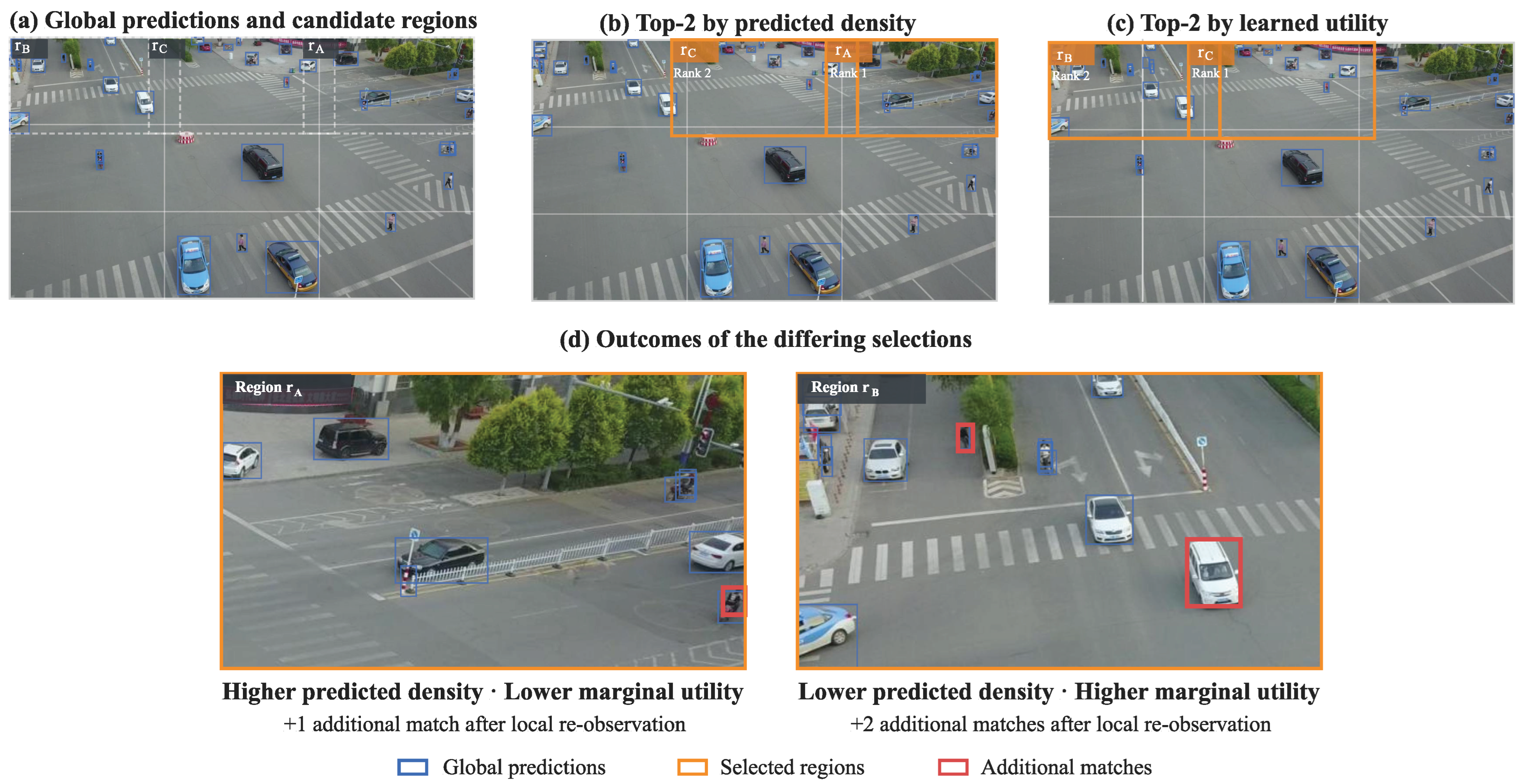
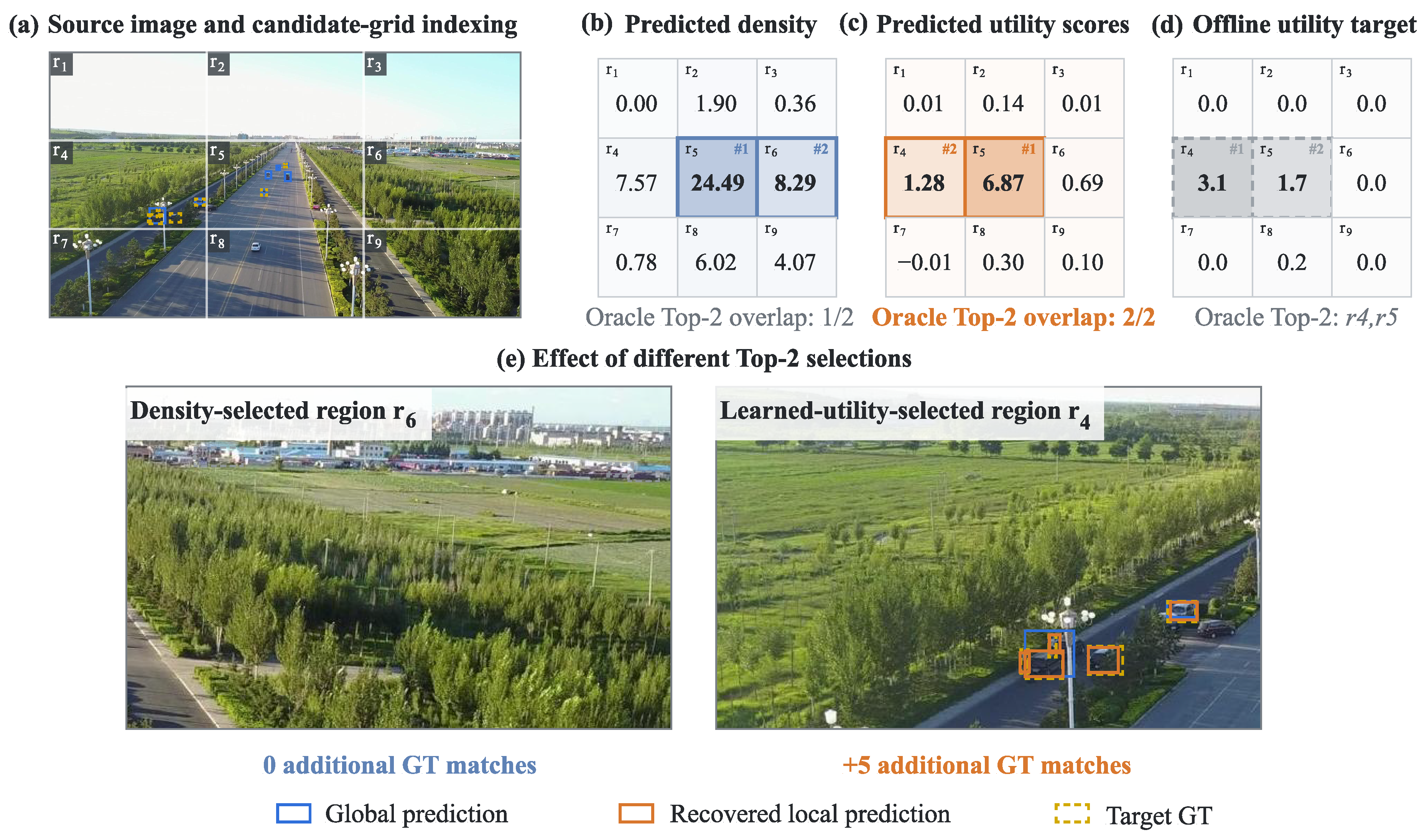
Target density and re-observation value are distinct. Predicted density measures target concentration within a candidate region. Re-observation value measures the detection evidence still missing after global inference. Dense regions with confident and well-localized detections may yield redundant local predictions; less dense regions may contain weak responses, incomplete evidence, or localization errors recoverable at higher local resolution. The global prediction state determines each candidate’s residual value. MRU estimates this residual value as the expected detection contribution of re-observing the region. Figure 1 contrasts density- and utility-based rankings and the detections recovered from their selected regions.

We present MRU-YOLO, a marginal-utility-guided framework for selective local re-observation. The implementation uses YOLO11n as the base detector and shares its weights across global and local inference. One global forward pass defines nine expanded candidate regions and supplies the detections used to construct their 26-dimensional prediction-conditioned states. Offline candidate processing provides multi-IoU supervision for learning the residual detection value of each region. During inference, a learned utility regressor ranks the candidates without annotations and selects the Top-2 regions for local processing. Source-aware fusion maps the local detections to the original image and integrates them with the global prediction set. The complete procedure operates outside the internal detector architecture and leaves the backbone, neck, and detection head unchanged.

The main contributions are as follows:

(1)

Prediction-conditioned marginal-utility learning. We combine a 26-dimensional candidate state with offline multi-IoU supervision to estimate residual regional value from global predictions. The learned selector ranks regions by the expected detection contribution of another local observation.

(2)

Budgeted selective local re-observation. Following one global pass, the policy ranks nine candidates and assigns the Top-2 observation budget to the highest-utility regions using shared detector weights. Online selection requires no annotations, no additional whole-image detector pass, and no modification to the detector architecture.

(3)

Source-aware fusion of global and local predictions. Original-coordinate size gating, local-score calibration, stable-global protection, and class-aware suppression preserve valid local recoveries while controlling duplicate boxes, confidence shifts, and crop-induced false positives.

Experiments on maritime and urban UAV datasets evaluate detection performance, regional ranking, observation allocation, fusion behavior, run-to-run variability, and computational characteristics.

2. Materials and Methods

2.1. Framework Overview

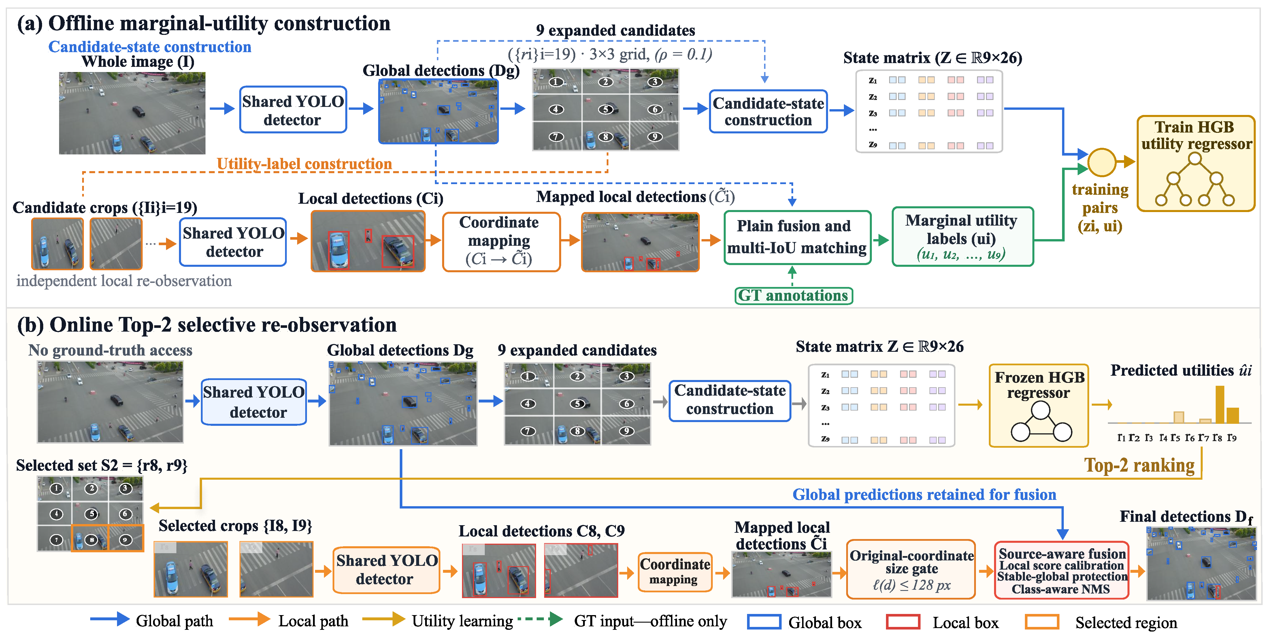
MRU-YOLO comprises an offline utility-learning stage and an online selective re-observation stage. Offline processing constructs candidate-wise supervision from independently evaluated crops. Online inference uses one global detector forward pass to rank candidate regions and processes the Top-K regions under a fixed observation budget. Figure 2 presents both workflows.

Let $I\in {\mathbb{R}}^{H\times W\times 3}$ denote a UAV image in original coordinates, and let $F_{\omega }$ denote a YOLO detector with fixed parameters [47]. The full image and selected local crops share the same detector weights. A global letterbox transform ${\mathcal{L}}_g$ resizes the full image to an input size of $s_g$. The detector produces predictions in the global letterbox coordinate system:

$${\mathcal{P}}_g=F_{\omega }\left({\mathcal{L}}_g(I;s_g)\right).$$

(1)

Here, $F_{\omega }$ denotes the complete prediction operator used by the evaluation protocol, including box decoding, confidence filtering, and class-aware non-maximum suppression (NMS) [48]. The inverse letterbox transform restores these predictions to the original-image coordinate system:

$${\mathcal{D}}_g={\mathcal{L}}_g^{-1}\left({\mathcal{P}}_g\right)={\left\{({\mathbf{b}}_j,p_j,c_j)\right\}}_{j=1}^{N_g}.$$

(2)

The inverse transform is applied element-wise to all boxes. Here, ${\mathbf{b}}_j=(x_{1j},y_{1j},x_{2j},y_{2j})$, $p_j$, and $c_j$ denote the bounding box, confidence, and class label of the jth global prediction. The original-coordinate set ${\mathcal{D}}_g$ supplies the information used to construct candidate states. The global letterbox set ${\mathcal{P}}_g$ supplies the global branch of formal fusion.

The method defines a finite candidate set $\mathcal{R}={\left\{r_i\right\}}_{i=1}^M$ in original-image coordinates. Each candidate has a prediction-conditioned state vector ${\mathbf{z}}_i$. A learned utility model predicts ${\widehat{u}}_i$ for each candidate. The online policy selects a fixed number of regions:

$${\mathcal{S}}_K=\underset{r_i\in \mathcal{R}}{arg\; TopK}{\widehat{u}}_i,\left|{\mathcal{S}}_K\right|=K.$$

(3)

The formal configuration uses $M=9$ and $K=2$. The budget specifies the number of crop images submitted to the local detector. Runtime is measured independently.

This formulation separates detector inference from observation allocation. The detector produces boxes, scores, and classes. The MRU component allocates local views after the global output becomes available. Learned utility and predicted density share the same candidates, detector weights, observation budget, and fusion procedure.

Figure 2 shows the availability of supervision across the two stages. Ground-truth annotations and exhaustive candidate processing are confined to offline utility construction. The online path uses global predictions, the frozen utility regressor, and selected crops. Section 2.2 defines the candidate state; Section 2.3 defines offline utility learning; Section 2.4 and Section 2.5 define online selection and fusion; Section 2.6, Section 2.7 and Section 2.8 specify data, implementation, and evaluation.

The two stages share the detector checkpoint and candidate geometry. Offline processing supplies one scalar utility label for every candidate. Online processing supplies one predicted score for every candidate and acquires the selected local views. This design keeps detector training, utility learning, and observation allocation as separate procedures.

2.2. Candidate Regions and Prediction-Conditioned State

MRU-YOLO uses a fixed candidate space for controlled comparison of region-selection signals. The original image is divided into a regular $3\times 3$ base grid with unrounded cell dimensions

$${\mathrm{\Delta }}_x={\displaystyle \frac{W}{3}},{\mathrm{\Delta }}_y={\displaystyle \frac{H}{3}}.$$

(4)

For horizontal index $a\in \{0,1,2\}$, the expanded integer pixel bounds are

$$\begin{array}{cc}\hfill x_1^{\left(a\right)}& =max\left(0,⌊(a-\rho ){\mathrm{\Delta }}_x⌋\right),\hfill \\ \hfill x_2^{\left(a\right)}& =min\left(W,⌈(a+1+\rho ){\mathrm{\Delta }}_x⌉\right).\hfill \end{array}$$

(5)

For vertical index $b\in \{0,1,2\}$, the corresponding bounds are

$$\begin{array}{cc}\hfill y_1^{\left(b\right)}& =max\left(0,⌊(b-\rho ){\mathrm{\Delta }}_y⌋\right),\hfill \\ \hfill y_2^{\left(b\right)}& =min\left(H,⌈(b+1+\rho ){\mathrm{\Delta }}_y⌉\right).\hfill \end{array}$$

(6)

The candidate region associated with grid position $(a,b)$ is

$$r_{a,b}=\left(x_1^{\left(a\right)},y_1^{\left(b\right)},x_2^{\left(a\right)},y_2^{\left(b\right)}\right).$$

(7)

The formal setting uses $\rho =0.1$. This parameter specifies per-side expansion relative to the unrounded base-cell width and height. Equations (5) and (6) implement integer rounding and image-boundary clipping. Boundary candidates can differ slightly in area and aspect ratio.

The fixed grid isolates the ranking signal from candidate generation. Every image presents nine decisions, and learned utility and predicted density operate on an identical search space.

Candidate expansion adds context near grid boundaries and reduces hard truncation of objects located close to a base-cell edge. Image-boundary clipping preserves valid pixel coordinates. The fixed layout also gives boundary and interior regions explicit geometric descriptors through area fraction, aspect ratio, and normalized bounds.

Global predictions are assigned to candidates according to box centers. For prediction ${\mathbf{b}}_j$, let $({\overline{x}}_j,{\overline{y}}_j)$ be its center. Candidate membership is

$$A_{ij}=⊮\left[x_{1i}\le {\overline{x}}_j\le x_{2i}\wedge y_{1i}\le {\overline{y}}_j\le y_{2i}\right].$$

(8)

Candidate membership uses inclusive coordinate tests. Overlapping candidates can share a global prediction and represent that target under different surrounding contexts.

Candidate $r_i$ is represented by a 26-dimensional prediction-conditioned state in the saved selector order:

$${\mathbf{z}}_i={\left[{\left({\mathbf{z}}_i^{\mathrm{loc}}\right)}^{\top },{\left({\mathbf{z}}_i^{\mathrm{img}}\right)}^{\top },{\left({\mathbf{z}}_i^{\det }\right)}^{\top },{\left({\mathbf{z}}_i^{\mathrm{cls}}\right)}^{\top }\right]}^{\top }\in {\mathbb{R}}^{11+4+9+2}={\mathbb{R}}^{26}.$$

(9)

The four feature groups describe candidate geometry, image context, local statistics of the global predictions, and predicted class composition.

Table 2. Ordered 26-dimensional candidate state used by the HGB utility regressor.

Group	No.	Feature	Definition
Candidate geometry	1	Candidate index	Zero-based index $q=i-1\in \{0,\dots ,8\}$ for region $r_i$.
	2	Grid size	Grid side length; 3 in the formal configuration.
	3	Horizontal grid index	q mod 3.
	4	Vertical grid index	$\lfloor q/3\rfloor$.
	5	Normalized left bound	$x_1/W$.
	6	Normalized top bound	$y_1/H$.
	7	Normalized right bound	$x_2/W$.
	8	Normalized bottom bound	$y_2/H$.
	9	Candidate area fraction	$(x_2-x_1)(y_2-y_1)/\left(WH\right)$.
	10	Candidate aspect ratio	$(x_2-x_1)/(y_2-y_1)$.
	11	Center distance	Euclidean distance from the normalized candidate center to $(0.5,0.5)$.
Image context	12	Image aspect ratio	$W/H$.
	13	Image width	Original width W (px).
	14	Image height	Original height H (px).
	15	Global prediction count	Predictions in the complete global set.
Detection statistics	16	Candidate prediction count	Prediction centers inside the candidate, including the boundary.
	17	Candidate prediction density	Candidate count per $10,000$ original-image candidate pixels.
	18	Mean confidence	Mean confidence of candidate-member predictions.
	19	Maximum confidence	Maximum confidence of candidate-member predictions.
	20	Confidence dispersion	Population standard deviation (ddof=0); zero for one prediction.
	21	Small-prediction count	Predictions with equivalent side $s\le 96$ px.
	22	Tiny-prediction count	Predictions with equivalent side $s\le 32$ px.
	23	Mean equivalent side	Mean $s=\sqrt{max(0,w_b)max(0,h_b)}$ (px).
	24	Maximum equivalent side	Maximum equivalent side s (px).
Class statistics	25	Class entropy	$-{\sum }_c{p}_{c}ln{p}_c$, using natural logarithms.
	26	Number of predicted classes	Distinct predicted classes inside the candidate.

provides the complete feature order and definitions. All box-derived quantities use original-image coordinates. Prediction density is measured per $10,000$ candidate pixels. Confidence dispersion uses the population standard deviation (ddof=0) and takes value zero for one prediction. Equivalent-side thresholds of 96 and 32 pixels define the small- and tiny-prediction counts. Class entropy uses the natural logarithm. Features 16–26 take value zero for an empty candidate; geometric and image-context features remain defined.

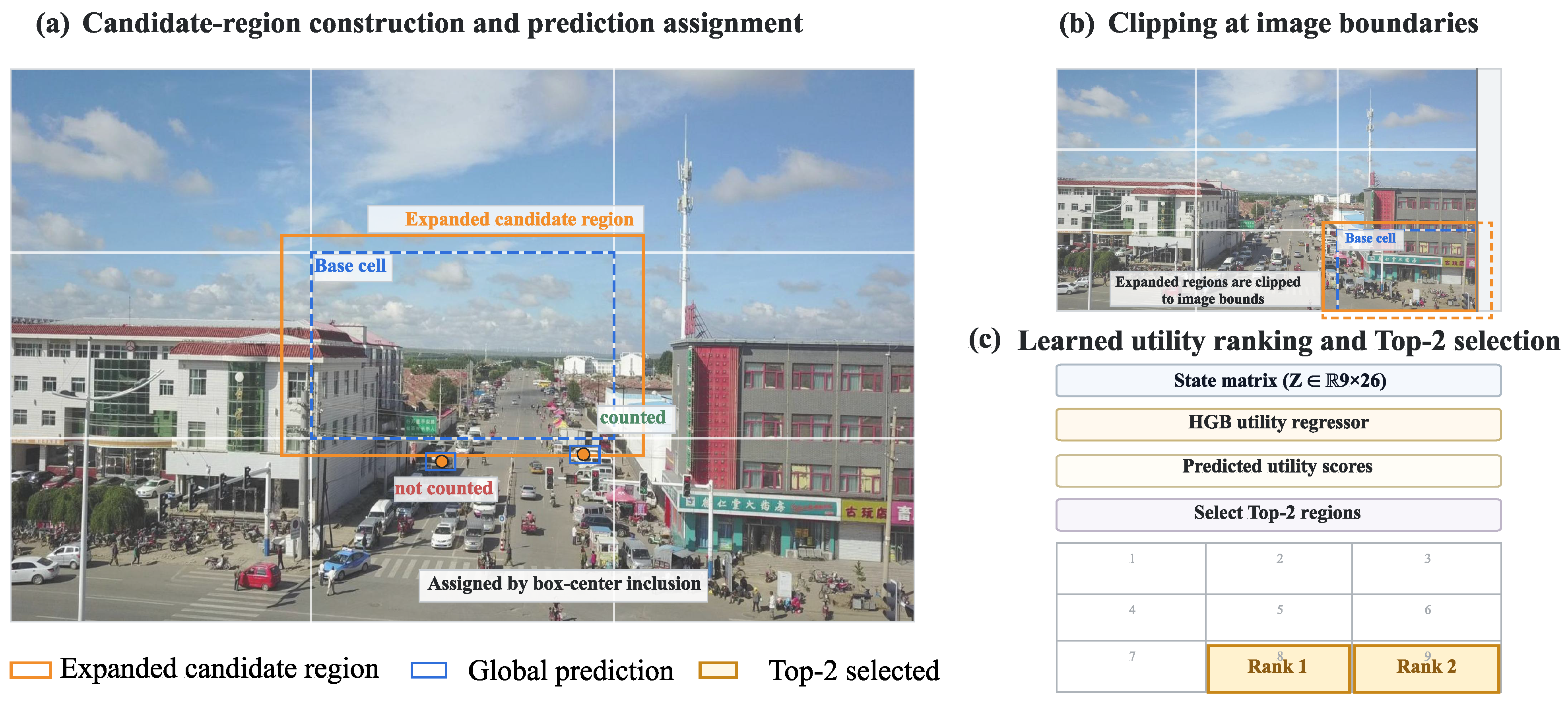
The state uses candidate geometry and information already available from global detection. Crop pixels, intermediate feature maps, annotation-derived attributes, and additional image-model outputs are absent from the representation. Learned utility uses the full state vector. Predicted-density selection uses feature 17 as its ranking score. Figure 3 visualizes candidate expansion, boundary clipping, center assignment, and Top-2 ranking.

The image-width and image-height features retain scene scale across heterogeneous source resolutions. The global prediction count supplies image-level context, and candidate-level count, confidence, equivalent-side, and class features summarize the local response of the global detector. The saved feature order is fixed during training and inference.

2.3. Offline Marginal-Utility Construction and Learning

The selector learns the value of a second observation from candidate-wise supervision. MRU-YOLO defines this value as the non-negative improvement in multi-IoU matched-detection quality produced by one independently processed candidate. Each training image first produces ${\mathcal{D}}_g$, followed by independent inference on all nine crops. Let ${\mathcal{L}}_i$ denote the local letterbox transform for candidate $r_i$, and let ${\mathbf{b}}_{ik}^{\mathrm{net}}$ denote its kth prediction in local network-input coordinates. Inverting the local transform gives crop-relative coordinates:

$${\mathbf{b}}_{ik}^{\mathrm{crop}}={\mathcal{L}}_i^{-1}\left({\mathbf{b}}_{ik}^{\mathrm{net}}\right).$$

(10)

The candidate-origin offset is

$${\mathbf{o}}_i={\left[x_{1i},y_{1i},x_{1i},y_{1i}\right]}^{\top }.$$

(11)

Adding this offset maps the prediction to original-image coordinates:

$${\tilde{\mathbf{b}}}_{ik}={\mathbf{b}}_{ik}^{\mathrm{crop}}+{\mathbf{o}}_i.$$

(12)

The mapped local prediction set for region $r_i$ is denoted ${\tilde{\mathcal{C}}}_i$. Boundary clipping removes invalid and zero-area boxes and preserves the alignment of boxes, confidence values, and class labels.

Candidate utility compares the global output with the result obtained after adding one independently processed crop. Plain fusion joins ${\mathcal{D}}_g$ and ${\tilde{\mathcal{C}}}_i$ using class-aware NMS:

$${\mathcal{D}}_{g\oplus i}^{\mathrm{plain}}={NMS}_{\mathrm{cls}}\left({\mathcal{D}}_g\cup {\tilde{\mathcal{C}}}_i;\eta ,N_{max}\right).$$

(13)

Utility-target construction uses $\eta =0.7$ and $N_{max}=1000$. Plain fusion performs coordinate-consistent combination and class-aware NMS. Formal inference uses the source-aware fusion policy defined in Section 2.5.

Let $\mathcal{G}$ be the ground-truth (GT) set and $\mathcal{T}=\{0.50,0.55,\dots ,0.95\}$ be the IoU threshold set. For prediction set $\mathcal{D}$, class-consistent one-to-one matching at each threshold gives a matched count $M_{\tau }(\mathcal{D},\mathcal{G})$. Candidate prediction–ground-truth pairs of the same class are sorted by decreasing IoU and greedily accepted. Each prediction and ground-truth object contributes to at most one match at each threshold. The multi-IoU quality proxy is

$$Q(\mathcal{D},\mathcal{G})={\displaystyle \frac{1}{\left|\mathcal{T}\right|}}\sum _{\tau \in \mathcal{T}}{M}_{\tau }(\mathcal{D},\mathcal{G}).$$

(14)

The independent marginal utility of region $r_i$ is the non-negative increment over the global result:

$$u_i=max\left[0,Q\left({\mathcal{D}}_{g\oplus i}^{\mathrm{plain}},\mathcal{G}\right)-Q\left({\mathcal{D}}_g,\mathcal{G}\right)\right].$$

(15)

The proxy supplies a candidate-ranking target based on class-consistent matched counts across IoU thresholds. Image-level AP supplies formal detection evaluation after multi-region selection and source-aware fusion. Each $u_i$ represents one candidate processed independently. Joint effects among selected crops enter the formal image-level output. The average across thresholds spans the AP50–95 evaluation range and remains a count-based regression target rather than AP itself. Section 3.4 evaluates the gap between independent Top-K ranking and a conditional oracle.

The average across ten IoU thresholds rewards both additional matches and localization quality. A recovered object contributes at lower thresholds first and continues to contribute at stricter thresholds as localization improves. The non-negative operator assigns zero utility to candidates whose plain-fusion matched count equals or falls below the global matched count. The resulting labels define an observation priority for each image. Section 3.4 also reports a controlled single-IoU ($\tau =0.50$) alternative.

The utility regressor $f_{\mathit{\theta }}$ maps the 26-dimensional state to this target:

$${\widehat{u}}_i=f_{\mathit{\theta }}\left({\mathbf{z}}_i\right).$$

(16)

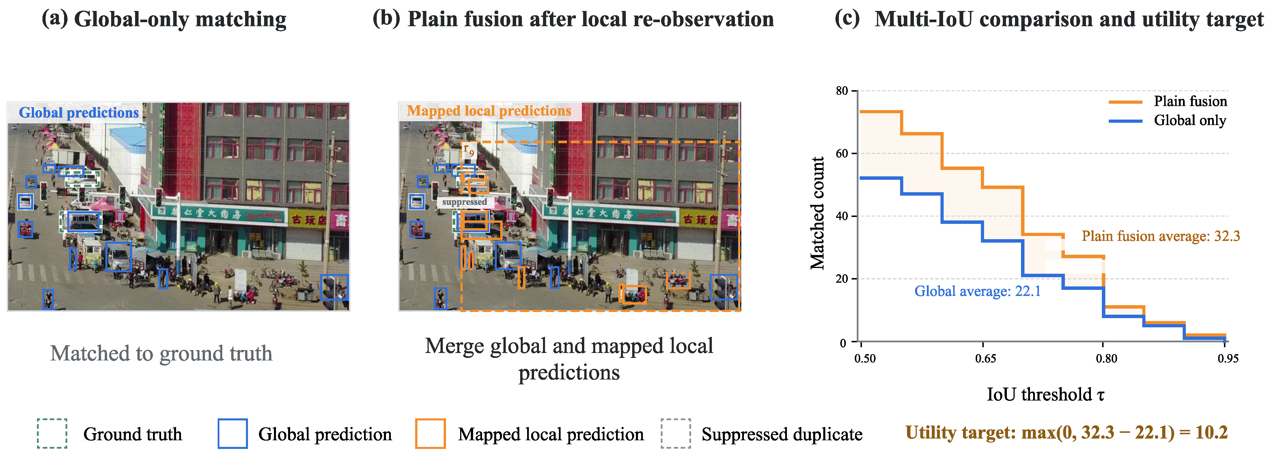
The implementation uses a histogram gradient boosting (HGB) regressor fitted on training-split state–utility pairs with scikit-learn [49]. Each image contributes nine independent candidate rows. Candidate-wise pointwise regression maps each 26-dimensional state to a scalar utility target. The regressor models non-linear interactions among position, confidence, size, density, and class composition. Validation utility labels support ranking diagnostics. Formal inference ranks the predicted utilities and selects the highest-scoring candidates. Figure 4 illustrates one offline label: plain fusion raises the mean matched count from 22.1 to 32.3 across the IoU thresholds, giving $u_i=10.2$.

The HGB model remains separate from the image detector and operates on a nine-row tabular input. Separate regressors capture the maritime and urban state distributions. The validation rows preserve an independent basis for utility capture, NDCG@2, and Oracle-overlap analysis.

2.4. Online Budgeted Local Re-Observation

At inference, MRU-YOLO stacks the nine candidate states into $\mathbf{Z}\in {\mathbb{R}}^{9\times 26}$. The frozen regressor scores all rows, and Equation (3) selects the highest-scoring candidates. The formal operating point is $K=2$; the budget sweep evaluates additional values of K. HGB regression scores are used only for ordering and are not clipped; exact ties are resolved by ascending candidate-window index.

The learned selector uses the global predictions and frozen HGB model. Predicted-density selection uses the same candidate states, detector weights, observation budget, and fusion procedure, with feature 17 as the ranking score.

This controlled substitution isolates the ranking signal. Candidate construction, local detector execution, coordinate recovery, and fusion remain fixed across the two deployable policies. The selector produces a complete ranking over all nine candidates before the Top-K budget is applied.

Each selected region is cropped from the original image and resized to the local detector input size. The crop uses the detector weights and evaluation settings of the global branch. Local processing increases the relative target scale and can recover evidence weakened by full-image resizing.

Equations (10)–(12) restore local predictions to original-image coordinates. Boundary clipping removes invalid and zero-area boxes. The observation budget counts selected crop inputs and excludes the mandatory global image. Runtime measurements report the implementation cost separately.

The crop branch preserves confidence values and class identities through coordinate recovery. The subsequent fusion stage receives the unchanged global prediction set and the restored predictions from all selected candidates.

2.5. Source-Aware Global–Local Fusion

Source-aware fusion combines global and local predictions through four ordered operations: local-size gating in original-image coordinates, mapping and score calibration in the global fusion space, stable-global protection, and final class-aware NMS. Global predictions retain their original scores. Local detector outputs begin in local network-input coordinates. Equations (10)–(12) restore them to original-image coordinates. The final protection and suppression operations use the global letterbox fusion space.

For a detection $d=(x_1,y_1,x_2,y_2,p,c)$, the box component is

$$\mathbf{b}\left(d\right)=(x_1,y_1,x_2,y_2).$$

(17)

Define $w\left(d\right)=max(0,x_2-x_1)$ and $h\left(d\right)=max(0,y_2-y_1)$. Its equivalent side length is

$$\ell \left(d\right)=\sqrt{w\left(d\right)h\left(d\right)}.$$

(18)

The function $\ell \left(·\right)$ uses the coordinate system of its argument. Mapped local detections are filtered according to original-image scale:

$$g_s\left(d\right)=⊮\left[\ell \left(d\right)\le {\tau }_s\right].$$

(19)

The formal setting uses ${\tau }_s=128$ original-image pixels. This gate confines local contributions to the target scale of re-observation.

The equivalent-side definition treats width and height symmetrically and provides one scale variable for boxes with different aspect ratios. The original-image coordinate system gives the threshold a consistent physical interpretation across local crops.

The confidence of each size-eligible local detection is calibrated by

$${\varphi }_{\alpha }\left(d\right)=\left(\mathbf{b}\left(d\right),\alpha p\left(d\right),c\left(d\right)\right).$$

(20)

The formal setting uses $\alpha =0.9$. Let ${\mathcal{V}}_g$ denote the deterministic mapping from original-image coordinates to the global letterbox fusion space. It preserves confidence and class. The selected local predictions form the union

$$\tilde{\mathcal{C}}=\bigcup _{i\in {\mathcal{S}}_K}{\tilde{\mathcal{C}}}_i.$$

(21)

The calibrated local pool is

$$\overline{\mathcal{C}}=\left\{{\varphi }_{\alpha }\left({\mathcal{V}}_g\left(d\right)\right):d\in \tilde{\mathcal{C}},g_s\left(d\right)=1\right\}.$$

(22)

The implementation applies scale gating, coordinate mapping, and score calibration in this order.

Score calibration aligns the locally enlarged predictions with the global score range before common suppression. Global scores retain their detector outputs throughout the fusion path.

Stable global predictions are defined in the global fusion coordinate system as

$${\mathcal{P}}_g^{\mathrm{stb}}=\left\{g\in {\mathcal{P}}_g:p\left(g\right)\ge {\tau }_g\wedge \ell \left(g\right)\ge {\tau }_{\ell }\right\}.$$

(23)

The formal setting uses ${\tau }_g=0.25$ and ${\tau }_{\ell }=96$ global-fusion pixels. For a calibrated local detection $d\in \overline{\mathcal{C}}$, the conflicting stable-global set is

$$\mathrm{\Omega }\left(d\right)=\left\{g\in {\mathcal{P}}_g^{\mathrm{stb}}:c\left(g\right)=c\left(d\right)\wedge IoU(g,d)\ge {\tau }_p\right\}.$$

(24)

The protection threshold is ${\tau }_p=0.5$. A calibrated local detection is retained when its conflict set is empty:

$${\mathcal{C}}^{*}=\left\{d\in \overline{\mathcal{C}}:\mathrm{\Omega }\left(d\right)=⌀\right\}.$$

(25)

The asymmetric rule removes conflicting local detections and preserves stable global detections.

Stable-global protection targets large, confident detections that already have strong global support. Class consistency and the IoU threshold restrict protection to spatially corresponding predictions of the same category. Smaller or lower-confidence global detections continue to compete with local detections in final NMS.

The global predictions and retained calibrated local predictions then enter class-aware NMS:

$${\mathcal{P}}_f={NMS}_{\mathrm{cls}}\left({\mathcal{P}}_g\cup {\mathcal{C}}^{*};\eta ,N_{max}\right).$$

(26)

The formal setting uses $\eta =0.7$ and $N_{max}=1000$. The final detections in original-image coordinates are obtained through the inverse relation

$${\mathcal{D}}_f={\mathcal{L}}_g^{-1}\left({\mathcal{P}}_f\right).$$

(27)

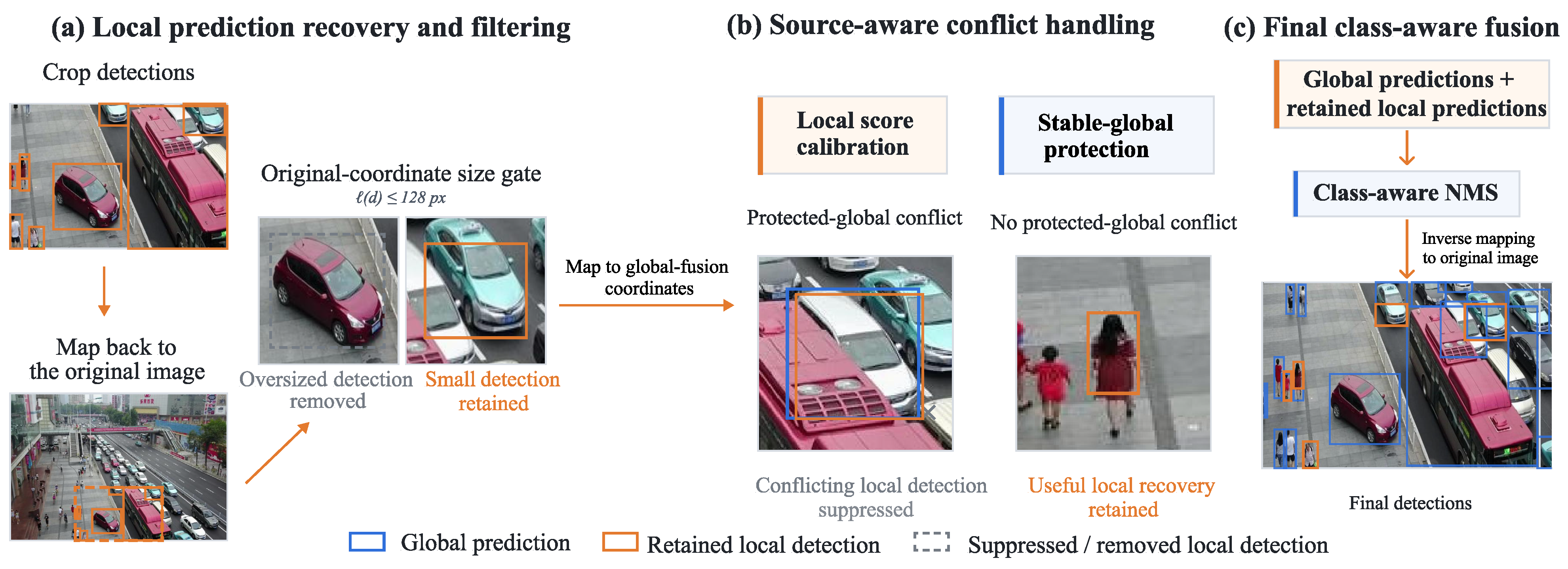
Equations (17)–(27) define the complete fusion operator. Figure 5 visualizes the ordered removal and retention of local detections. The controlled ablation fixes coordinate recovery, prediction mapping, global–local combination, and final class-aware NMS; it compares plain fusion with the joint source-aware policy.

Utility-target construction and formal inference use separate fusion operators. Plain fusion constructs candidate labels from one crop at a time. Source-aware fusion integrates the selected crop set and applies the calibrated protection policy.

Plain fusion constructs labels from the isolated contribution of each candidate, excluding set-dependent protection and score calibration from the regression target. Source-aware fusion integrates the selected crop set at inference, when cross-source conflicts can be resolved jointly. Section 3.4 evaluates a source-aware alternative for constructing single-crop labels.

The online path comprises one global detector forward pass, construction of nine candidate states, one HGB inference pass over nine rows, K selected crop inputs, coordinate recovery, source-aware filtering, and final NMS. Section 3.6 reports the measured implementation time.

2.6. Datasets and Data Preparation

The evaluation uses SeaDronesSee ODv2 as the primary maritime dataset [50] and VisDrone2019-DET as an independent urban dataset [51]. SeaDronesSee contains swimmers, boats, jetskis, life-saving appliances, and buoys under substantial scale variation. Its training and validation sets contain 8930 and 1547 images. VisDrone contains pedestrians, people, bicycles, cars, vans, trucks, tricycles, awning-tricycles, buses, and motors. Its official training and validation splits contain 6471 and 548 images.

The VisDrone conversion retains original categories 1–10 and maps them to zero-based classes 0–9. Original category 0 marks ignored regions, and category 11 represents others; both categories are excluded from the converted YOLO labels. Ignored regions are absent from evaluator masks. The evaluator uses the converted ten-class labels. The reported VisDrone values are Ultralytics validation metrics for this label set. Official test-dev, test-challenge, and server scores lie outside this evaluation.

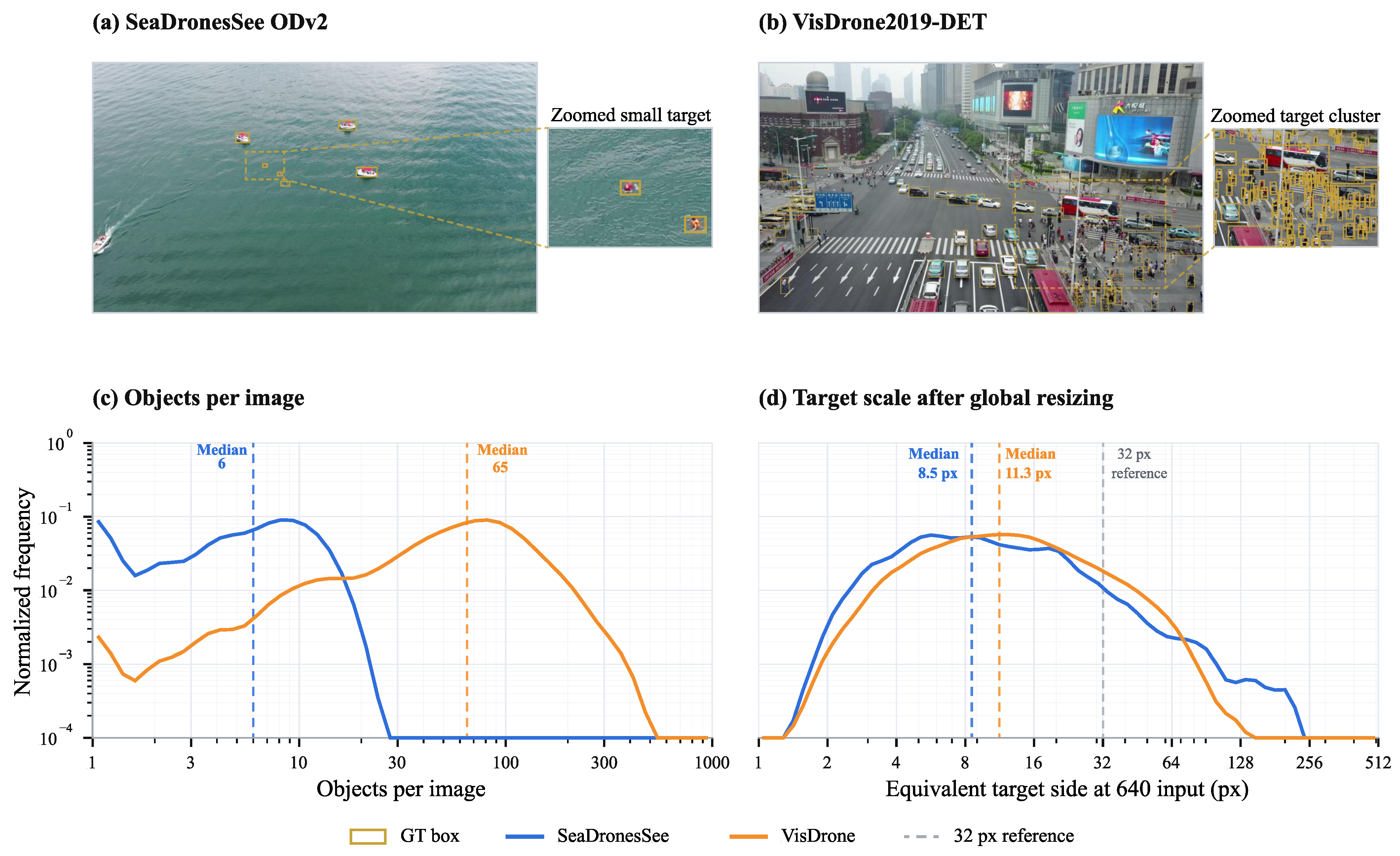
Separate detector and selector models are trained for the maritime and urban datasets. Figure 6 presents representative scenes, object-count distributions, and target scales after resizing to a 640-pixel global input. SeaDronesSee has a median of 6 objects per image and a median equivalent target side of 8.5 pixels. The corresponding VisDrone medians are 65 objects and 11.3 pixels.

Table 3. Dataset characteristics and common evaluation protocol. Panel and column headings are bold for structural formatting.

(a) Dataset Characteristics
Dataset	Scenario	Train	Validation	Classes	Median GT/Image	Median Side at 640 px
SeaDronesSee ODv2	Maritime	8930	1547	5	6	8.5
VisDrone2019-DET	Urban	6471	548	10	65	11.3
(b) Common Evaluation Protocol
Setting	Value			Setting		Value
Global input	640 px			Local input		640 px
Candidates	$3\times 3$			Expansion ratio		$\rho =0.1$
Local budget	Top-2			Confidence threshold		0.001
NMS IoU	0.70			Maximum detections		1000
Detector precision	FP16			Final fusion		Source-aware
Online selection	One global pass; no GT			Hardware		RTX 3090

a consolidates the split sizes, class counts, and distribution summaries.

The two datasets provide complementary operating conditions. SeaDronesSee emphasizes sparse maritime targets against large water backgrounds. VisDrone emphasizes dense urban layouts with frequent occlusion and many compact instances. Both datasets retain small median target scales after global resizing.

2.7. Training and Implementation Details

The SeaDronesSee and VisDrone detectors are trained independently for 150 epochs with a batch size of 16 and eight data-loading workers. Optimization uses stochastic gradient descent (SGD) with an initial learning rate of 0.01, a cosine schedule, and a final learning-rate factor of 0.01. Three complete detector–selector runs were conducted using detector-training seeds 0, 1, and 2. Automatic mixed precision is enabled, and training uses the default non-deterministic execution mode. Training uses mosaic, scale, and erasing settings of 1.0, 0.4, and 0.4, respectively. Mosaic augmentation is disabled during the final 15 epochs. Evaluation uses the checkpoint with the best validation performance.

Each dataset has a separate HGB utility regressor with 300 boosting iterations, a learning rate of 0.05, ${\ell }_2$ regularization of 0.01, and random state 0. Every training image contributes nine 26-dimensional state–utility rows. Training-split rows fit the regressor, and validation-split rows support ranking diagnostics.

Detector training and selector training use their corresponding dataset splits. The detector checkpoint generates the global and crop predictions used for state construction, utility-label generation, formal validation, and timing.

The software environment comprises Python 3.11.15, PyTorch 2.7.1 with CUDA 12.6, Ultralytics 8.4.50, cuDNN 90501, and OpenCV 4.13.0. Training, formal validation, and timing measurements use an NVIDIA GeForce RTX 3090. Global and crop detector calls during formal online evaluation use 16-bit floating-point inference (FP16). Offline utility construction and CPU selector execution use their recorded default precision settings.

2.8. Evaluation Protocol and Ranking Diagnostics

All formal MRU runs use global and local input sizes of 640 pixels, a confidence threshold of 0.001, a class-aware NMS IoU threshold of 0.70, and $N_{max}=1000$. The maximum-detection setting accommodates dense aerial images with more than 300 detections. The candidate space uses the expanded $3\times 3$ grid with $\rho =0.1$, and the formal configuration uses a Top-2 observation budget. Learned utility and predicted density share the validation split, detector checkpoint, candidates, observation budget, and fusion procedure. Table 3b lists the common protocol.

The formal protocol applies FP16 to global and selected-crop detector calls. One global forward pass supplies the candidate states for each image. The selected crop count defines the local observation budget. The repeatability study uses the same protocol for all three seeds and reports sample means and sample standard deviations.

YOLO11n-640 is the matched lightweight baseline and supplies the global prediction state used by MRU-YOLO. For each seed, global-only, MRU, and SAHI inference use the same detector checkpoint and validation protocol, isolating the effect of selective local re-observation from detector scaling.

Formal detection evaluation reports Precision, Recall, mAP50, and mAP50–95 from complete image-level outputs after selection and fusion. Metric values are percentages, and differences are percentage points. Baseline reevaluations use existing checkpoints and the confidence threshold, NMS IoU threshold, maximum-detection limit, inference precision, and validation settings of the corresponding MRU runs.

Offline ranking evaluation reports utility capture and NDCG@2 [52]. For an image x, utility capture is the sum of the non-negative proxy utilities of the policy-selected Top-2 candidates divided by the Oracle Top-2 sum. NDCG@2 uses the same independent-candidate proxy utility as the relevance score, applies logarithmic discounting in policy order, and normalizes by the Oracle ordering.

The reported means use images with positive Oracle Top-2 utility. This set contains 1141 of 1547 SeaDronesSee validation images and 532 of 548 VisDrone validation images. Utility capture and NDCG@2 measure agreement with the offline candidate-ranking target. Formal detection metrics measure the complete output of selection and fusion.

Oracle Top-2 sorts candidates by the saved independent-candidate utility labels. Utility capture measures recovered cumulative utility, and NDCG@2 measures order-sensitive ranking quality. The positive-Oracle subset supplies a defined denominator for both metrics. Center-prior ranks candidates by increasing the Euclidean distance between their normalized centers and $(0.5,0.5)$. GT small-object-count ranks candidates by the number of validation ground-truth objects whose centers lie inside the candidate and whose equivalent side is at most 96 original-image pixels; it is an offline privileged-information diagnostic and is not deployable. Random ranking samples a uniformly random ordering of the nine candidates 1000 times; the reported random values are means with empirical 95% intervals.

Runtime evaluation uses CUDA-synchronized, single-image FP16 inference on the RTX 3090. Each route receives 30 warm-up images followed by 300 timed images. Runtime evaluation reports total end-to-end latency, including preprocessing, state construction or slicing, detector calls, fusion, and final NMS. Disk I/O and external deployment-framework overhead are outside the timed path.

The route-level detection mAP50–95 values are averaged over three independent runs. Runtime values are synchronized FP16 batch-1 measurements obtained with the checkpoint corresponding to seed 0 and are reported as mean ± sample standard deviation over five timing repetitions.

Unless otherwise specified, the analyses in Section 3.4, Section 3.5 and Section 3.6 use the detector–selector chain corresponding to seed 0.

The SAHI reference uses SAHI v0.12.1 with $640\times 640$ slices, height and width overlap ratios of 0.20, and standard full-image prediction enabled. Its post-processing is class-aware NMS with IoU threshold 0.50; detector confidence is 0.001, detector NMS IoU is 0.70, $N_{max}=1000$, FP16 is enabled, and the slice batch size is one. The reported detector inputs per image equal the standard full-image input plus the resolution-dependent number of slices, which explains the different dataset averages. SAHI detection accuracy is averaged over the three matched checkpoints; its runtime statistics use five repetitions with the checkpoint corresponding to seed 0.

3. Results

3.1. Overall Detection Performance

Table 4. Overall detection performance on SeaDronesSee ODv2 and VisDrone2019-DET. Bold indicates the MRU-YOLO method and the highest mean mAP50–95 value within each dataset.

Dataset	Method	P (%)	R (%)	mAP50 (%)	mAP50–95 (%, Mean ± SD)	Local Crops/ Image	ΔmAP50–95 (pp)
SeaDronesSee ODv2	YOLO11n-640 (global)	83.69	68.06	69.55	$39.50\pm 0.08$	0	0.00
	Predicted density (Top-2)	75.43	70.07	72.73	$41.78\pm 0.36$	2	+2.29
	MRU-YOLO (Top-2)	75.40	70.10	72.86	41.82 ± 0.34	2	+2.32
VisDrone2019-DET	YOLO11n-640 (global)	45.19	33.93	32.87	$18.45\pm 0.10$	0	0.00
	Predicted density (Top-2)	46.05	39.62	37.71	$21.69\pm 0.06$	2	+3.24
	MRU-YOLO (Top-2)	46.07	39.77	37.78	21.72 ± 0.07	2	+3.28

compares MRU-YOLO with the matched YOLO11n-640 global detector and predicted-density selection. The matched detector and fixed Top-2 observation budget isolate the contribution of the regional ranking policy, and the reported route-level values are means across three runs.

MRU-YOLO consistently improved detection accuracy in both maritime and urban UAV scenes; Table 4 reports the variation across runs.

Learned utility and predicted density achieved similar final detection accuracy; learned utility consistently aligned more closely with the offline utility target.

3.2. Class-Wise and Qualitative Results

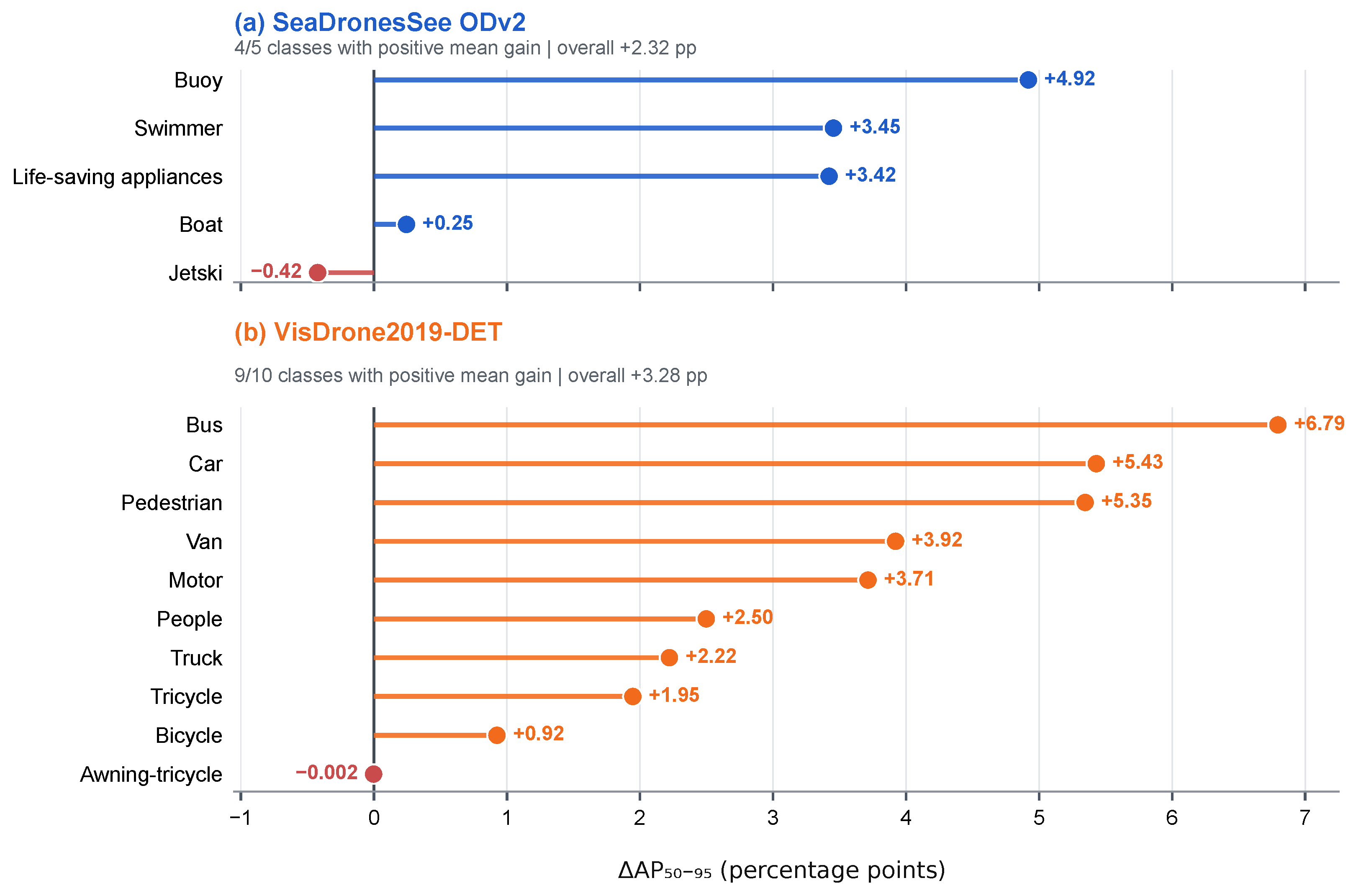
The class-wise SeaDronesSee results, averaged across three runs, showed that the aggregate gain was concentrated in small and visually weak maritime targets. Four of the five classes improved in AP50–95. Buoy recorded the largest increase at 4.92 percentage points, followed by swimmer at 3.45 percentage points and life-saving appliances at 3.42 percentage points. AP50–95 increased by 0.25 percentage points for boat and decreased by 0.42 percentage points for jetski. Figure 7a presents the full class-wise distribution.

Averaged across three runs, nine of the ten VisDrone classes achieved positive mean gains over the matched global baseline. Bus, car, pedestrian, and van produced the largest gains, reaching 6.79, 5.43, 5.35, and 3.92 percentage points, respectively. The awning-tricycle class was effectively unchanged, with a difference of $-0.002$ percentage points. Figure 7b summarizes this cross-class pattern.

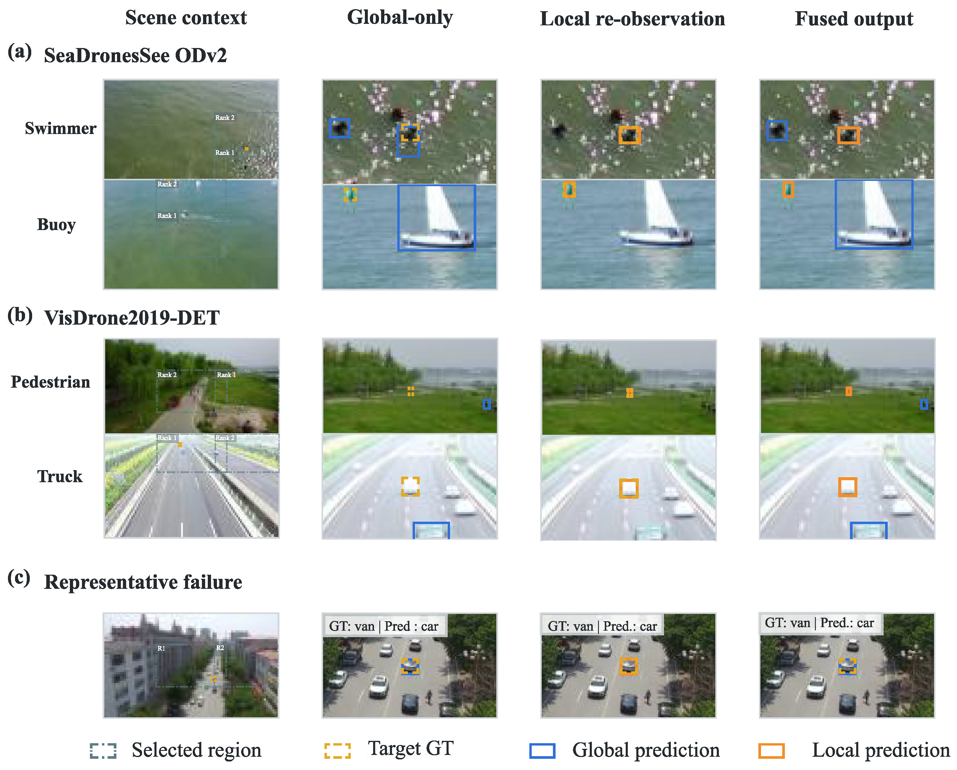
Figure 8 provides detection-level examples from both datasets. Local re-observation recovered a swimmer and a buoy in the SeaDronesSee scenes. It also recovered a pedestrian and a truck in the VisDrone scenes. The final fused outputs retained the relevant global detections and incorporated the recovered local targets. The van remained misclassified as a car after global detection, local re-observation, and fusion. Added spatial detail alone did not resolve this semantic confusion.

3.3. Selection Performance and Ranking Quality

Table 5. Detection performance and offline Top-2 ranking diagnostics. Bold values indicate the higher value between the two selection policies for each dataset and offline ranking metric.

(a) Detection Performance
Dataset	Method	mAP50–95 (%)	$\mathrm{\Delta }$ vs. Global Only (pp)	$\mathrm{\Delta }$ vs. Predicted Density (pp)
SeaDronesSee ODv2	Global only	39.496	–	–
	Predicted density (Top-2)	41.784	+2.289	–
	Learned utility (Top-2)	41.819	+2.323	+0.035
VisDrone2019-DET	Global only	18.446	–	–
	Predicted density (Top-2)	21.690	+3.245	–
	Learned utility (Top-2)	21.725	+3.279	+0.035
(b) Offline Ranking Diagnostics
Dataset	Selection Policy	Utility Capture (%)	NDCG@2 (%)	Evaluation Subset (Oracle Top-2 Utility > 0)
SeaDronesSee ODv2	Predicted density	83.74	80.16	1141/1547 images
	Learned utility	84.94	81.13
VisDrone2019-DET	Predicted density	84.19	83.04	532/548 images
	Learned utility	89.36	88.79

reports final detection accuracy and offline ranking quality under the same Top-2 observation budget. Utility capture measures the fraction of positive Oracle Top-2 utility recovered by a policy. NDCG@2 measures the agreement between its ranked candidates and the marginal-utility target. Both diagnostics are averaged over images with positive Oracle Top-2 utility. Panel (a) reports final detection accuracy across three complete detector–selector runs; panel (b) reports seed-0 offline ranking quality.

Across three runs, both Top-2 policies outperformed global-only detection. Learned utility increased mAP50–95 by 2.323 percentage points on SeaDronesSee and 3.279 percentage points on VisDrone, exceeding predicted density by 0.035 percentage points on both datasets.

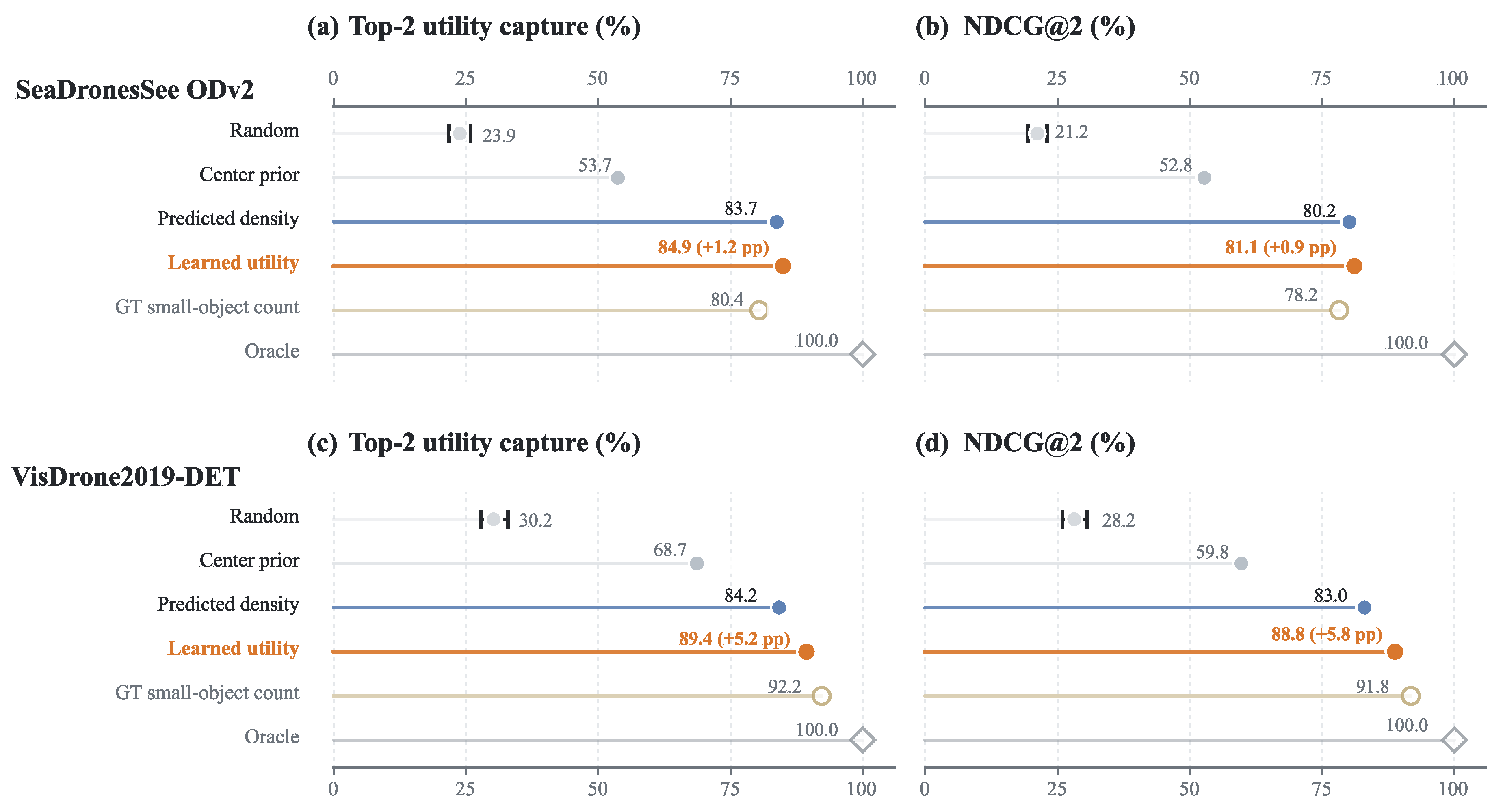
The offline ranking metrics consistently favored learned selection. On SeaDronesSee, learned selection reached 84.94% utility capture and 81.13% NDCG@2, compared with 83.74% and 80.16% for predicted density. On VisDrone, the corresponding values were 89.36% and 88.79% for learned selection and 84.19% and 83.04% for predicted density. The learned selector achieved closer agreement with the marginal-utility supervision target on both datasets.

Figure 9 places the two deployable policies alongside center-prior, random, GT small-object count, and Oracle rankings. The learned policy exceeded predicted density in both ranking metrics, with the largest separation on VisDrone.

Figure 10 presents one VisDrone disagreement case. Learned utility selected $r_5$ and $r_4$, matching the Oracle pair. Predicted density selected $r_5$ and $r_6$. Re-observation of $r_4$ added five matched targets, compared with zero for $r_6$. This spatial example complements the dataset-level ranking statistics.

3.4. Selector Robustness

Table 6. Controlled ablations and hyperparameter sensitivity.

(a) Controlled Ablations
Component	Configuration	SeaDronesSee		VisDrone
		mAP50–95 (%)	Δ vs. Ref. (pp)	mAP50–95 (%)	Δ vs. Ref. (pp)
State Representation	Full 26-dimensional state	41.68	0.00	21.80	0.00
	Without detection- statistics features	41.37	−0.31	21.20	−0.60
	Prediction-only state	41.79	+0.11	21.77	−0.04
Utility Target	Multi-IoU mean matched count	41.68	0.00	21.80	0.00
	Matched count at IoU $=0.50$	41.76	+0.08	21.84	+0.04
Label-Construction Fusion	Plain fusion	41.71	0.00	21.82	0.00
	Source-aware fusion	41.72	+0.01	21.81	−0.01
Inference-Time Fusion	Plain direct fusion	39.90	0.00	21.47	0.00
	Joint source-aware fusion	41.68	+1.78	21.80	+0.33
(b) Hyperparameter Sensitivity
Dataset	Within 0.5 pp	Total Tested	Most Sensitive Parameter	Tested Value	ΔmAP50–95 (pp)
SeaDronesSee ODv2	15	18	Fusion NMS IoU threshold	0.90	−1.37
VisDrone2019-DET	14	18	Fusion NMS IoU threshold	0.90	−1.17

summarizes controlled ablations and hyperparameter sensitivity. The reduced state without detection-statistics features retains features 1–15 and 25–26, whereas the prediction-only state uses features 16–26. Removing detection-statistics features reduced mAP50–95 by 0.31 percentage points on SeaDronesSee and 0.60 percentage points on VisDrone. The prediction-only selector performed similarly to the full representation. Detector-derived statistics supplied the dominant utility signal, with smaller, dataset-dependent contributions from geometric and image-context descriptors. For each fusion setting, labels and the corresponding selector were generated separately under matched detector and inference conditions.

Source-aware and plain label construction produced nearly identical final mAP50–95, differing by +0.01 percentage points on SeaDronesSee and −0.01 percentage points on VisDrone.

With the detector, selector, selected regions, and Top-2 budget fixed, joint source-aware fusion increased mAP50–95 by 1.78 percentage points on SeaDronesSee and 0.33 percentage points on VisDrone.

Replacing the multi-IoU proxy with an IoU = 0.50 matched-count target changed final mAP50–95 by at most 0.08 percentage points. Both targets produced comparable final accuracy; the multi-IoU target spans the AP50–95 evaluation range. Of the 18 alternatives, 15 configurations on SeaDronesSee and 14 on VisDrone remained within 0.5 percentage points of the reference. Only the 0.90 fusion NMS threshold and the $4\times 4$ grid fell outside this band on both datasets. Removing score calibration fell outside the band only on SeaDronesSee, whereas $K=1$ and zero overlap did so only on VisDrone.

An offline conditional Top-2 oracle evaluated the dependence of the second crop on the first. Conditional selection improved mAP50–95 over independent ranking by 0.10 percentage points on SeaDronesSee and 0.12 percentage points on VisDrone and remained within 0.01 percentage points of exhaustive pair selection on both datasets. These gaps show that independent ranking closely approximates conditional selection under the fixed Top-2 budget.

3.5. Observation-Budget Analysis

Table 7. Detection performance across local observation budgets. Bold indicates the formal operating point used in the main experiments.

Observation Budget	Local Crops/ Image	SeaDronesSee mAP50–95 (%)	VisDrone mAP50–95 (%)
Top-1	1	41.18	21.25
Top-2	2	41.68	21.80
Top-3	3	41.69	22.04
Top-4	4	41.82	22.09
All 9 candidates	9	41.72	21.54

evaluates learned selection across $K=1$–4 and the all-candidate reference using the same learned selector, $3\times 3$ candidate space, source-aware fusion, and controlled ablation protocol. Additional crops produced only small, dataset-dependent changes; processing all nine candidates did not outperform Top-2 on either dataset.

3.6. Scene-Density and Computational Analysis

Table 8. Density-stratified changes in mAP50–95 from global detection to MRU-YOLO (Top-2). Bold indicates the largest mAP50–95 gain within each dataset’s density strata.

Dataset	Density Stratum	Images	Mean GT/Image	ΔmAP50–95 (pp)
SeaDronesSee	Low	515	2.13	$-0.17$
SeaDronesSee	Mid	516	6.18	+3.20
SeaDronesSee	High	516	10.35	+1.42
VisDrone	Low	182	26.71	+2.11
VisDrone	Mid	183	65.81	+3.15
VisDrone	High	183	119.42	+3.89

evaluates MRU-YOLO across scene-density strata. Each validation set was divided into three equal-count groups according to the number of ground-truth objects per image. The values report changes from global detection to learned Top-2 re-observation within each group. These strata characterize image-level object density and remain distinct from COCO object-size categories [53].

MRU-YOLO achieved positive mAP50–95 gains in the medium- and high-density SeaDronesSee groups and across all three VisDrone groups. MRU-YOLO decreased mAP50–95 by 0.17 percentage points in low-density SeaDronesSee scenes, compared with gains of 3.20 percentage points in medium-density SeaDronesSee scenes and 3.89 percentage points in high-density VisDrone scenes. Gains were concentrated in the medium- and high-density strata.

Table 9. Accuracy and computational cost of matched inference routes on an RTX 3090. Bold indicates the highest mAP50–95 value within each dataset.

Dataset	Route	mAP50–95 (%)	Detector Inputs/Image	Nominal Detector GFLOPs	End-to-End Latency (ms)	FPS	Peak CUDA Memory (MB)
SeaDronesSee ODv2	YOLO11n-640 (global)	39.50	1.00	6.32	$11.57\pm 0.80$	86.40	48.13
	MRU-YOLO (Top-2)	41.82	3.00	18.95	$32.40\pm 1.21$	30.86	61.07
	SAHI (NMS/IoU)	34.62	33.64	212.53	$587.93\pm 21.03$	1.70	58.70
VisDrone2019-DET	YOLO11n-640 (global)	18.45	1.00	6.32	$10.33\pm 0.33$	96.83	48.12
	MRU-YOLO (Top-2)	21.72	3.00	18.95	$30.09\pm 2.44$	33.24	61.19
	SAHI (NMS/IoU)	21.50	6.19	39.11	$167.06\pm 5.14$	5.99	58.71

reports computational reference measurements and end-to-end route comparisons on an RTX 3090 under synchronized single-image FP16 execution.

MRU-YOLO uses one global detector input and two selected local inputs per image, giving a fixed detector workload of 18.95 nominal GFLOPs for YOLO11n-640. The end-to-end throughput was 30.86 FPS on SeaDronesSee and 33.24 FPS on VisDrone, with peak CUDA memory of 61.07 and 61.19 MB, respectively. The SAHI NMS/IoU route used 33.64 and 6.19 detector inputs per image and reached 1.70 and 5.99 FPS. Its mean mAP50–95 values across three runs were 34.62% and 21.50%, respectively. These measurements demonstrate that MRU-YOLO uses a fixed, substantially smaller detector-call budget than the evaluated slicing reference.

4. Discussion

The results demonstrate that selective re-observation can recover fine-grained evidence without distributing additional processing uniformly across the image. MRU-YOLO improved the matched global detector in both maritime and urban UAV scenes, with class-wise gains concentrated on targets whose evidence is easily weakened by global resizing. The density-stratified results showed larger gains in the medium- and high-density strata than in the low-density stratum. The qualitative examples show representative recoveries and a persistent van-to-car confusion; image-level metrics quantify overall performance. These findings identify spatial allocation as a central factor in global–local detection. Increasing image resolution or model capacity enhances representations throughout the image, whereas selective re-observation concentrates additional detail on regions that remain informative after global inference.

Marginal re-observation utility provides the decision signal required by this allocation process. Predicted density measures where objects are concentrated, whereas marginal utility measures the expected contribution of observing a region again. The learned selector achieved higher utility capture and NDCG@2 on both datasets, aligning more closely with the offline marginal-utility target than predicted density. The similar final AP values indicate that crop inference and source-aware fusion also govern end-to-end accuracy. Region selection determines which evidence becomes available; crop inference and source-aware fusion determine how effectively that evidence contributes to the final prediction. MRU-YOLO links these stages in a unified pipeline that selects regions according to expected incremental value and integrates their detections according to source-specific characteristics.

The budget and fusion analyses show that effective local processing depends on both observation placement and evidence integration. Top-2 is the fixed operating point. Increasing the budget to Top-3 or Top-4 changed mAP50–95 only modestly, and processing all nine candidates did not outperform Top-2 on either dataset. Source-aware fusion improved detection accuracy by coordinating recovered local evidence with global predictions. Relative to plain direct fusion, the joint policy improved mAP50–95 by 1.78 and 0.33 percentage points on SeaDronesSee and VisDrone, respectively. These components operate outside the internal detector architecture and require only global predictions, selected image regions, and mapped local detections. This inference-level design preserves the detector backbone, neck, and head and uses standard detector outputs for region selection and fusion. The conditional oracle improved mAP50–95 over independent Top-2 ranking by 0.10 and 0.12 percentage points, showing that independent ranking closely approximates conditional selection. Results from independently trained maritime and urban systems establish marginal utility as a practical signal for allocating local visual computation.

Future work could extend MRU-YOLO in three directions. First, the fixed Top-2 observation budget could be replaced by an adaptive policy that changes the number of local observations according to scene complexity and computational constraints. Second, marginal-utility estimation could be extended from single images to video-based UAV perception, where temporal consistency may provide additional cues for region selection and fusion. Finally, lightweight utility predictors and deployment-oriented fusion strategies could further reduce inference overhead for real-time onboard applications.

5. Conclusions

This paper presents MRU-YOLO, a marginal-utility-guided framework for selective local re-observation in UAV small-object detection. The framework estimates the incremental value of candidate regions from global predictions, assigns a limited observation budget to the highest-value regions, and integrates global and local detections through source-aware fusion. Across three independent runs, MRU-YOLO achieved mean mAP50–95 gains of 2.32 and 3.28 percentage points over the matched YOLO11n-640 baseline on SeaDronesSee ODv2 and VisDrone2019-DET, respectively.

MRU-YOLO improved AP50–95 in four of five maritime categories and nine of ten urban categories; the remaining urban category was effectively unchanged. Ranking analysis shows that learned utility aligns more closely with the marginal-utility target than predicted density. The ablations quantify the observation-budget trade-off and verify the contribution of source-aware fusion. MRU-YOLO operates on detector predictions and image regions without redesigning the detector backbone, neck, or head. It directs local computation toward regions with the highest expected contribution after global detection, providing a prediction-conditioned alternative to uniform spatial processing in UAV detection.

References

1. Mohsan, S.A.H.; Khan, M.A.; Noor, F.; Ullah, I.; Alsharif, M.H. Towards the Unmanned Aerial Vehicles (UAVs): A Comprehensive Review. Drones 2022, 6, 147. [Google Scholar] [CrossRef]
2. Yang, T.; Jiang, Z.; Sun, R.; Cheng, N.; Feng, H. Maritime Search and Rescue Based on Group Mobile Computing for Unmanned Aerial Vehicles and Unmanned Surface Vehicles. IEEE Trans. Ind. Inform. 2020, 16, 7700–7708. [Google Scholar] [CrossRef]
3. Nikouei, M.; Baroutian, B.; Nabavi, S.; Taraghi, F.; Aghaei, A.; Sajedi, A.; Moghaddam, M.E. Small Object Detection: A Comprehensive Survey on Challenges, Techniques and Real-World Applications. Intell. Syst. Appl. 2025, 27, 200561. [Google Scholar] [CrossRef]
4. Yu, X.; Gong, Y.; Jiang, N.; Ye, Q.; Han, Z. Scale Match for Tiny Person Detection. In Proceedings of the 2020 IEEE Winter Conference on Applications of Computer Vision, Snowmass, CO, USA, 1–5 March 2020; pp. 1246–1254. [Google Scholar] [CrossRef]
5. Wang, X.; Wang, A.; Yi, J.; Song, Y.; Chehri, A. Small Object Detection Based on Deep Learning for Remote Sensing: A Comprehensive Review. Remote Sens. 2023, 15, 3265. [Google Scholar] [CrossRef]
6. Tang, G.; Ni, J.; Zhao, Y.; Gu, Y.; Cao, W. A Survey of Object Detection for UAVs Based on Deep Learning. Remote Sens. 2024, 16, 149. [Google Scholar] [CrossRef]
7. Ni, J.; Zhu, S.; Tang, G.; Ke, C.; Wang, T. A Small-Object Detection Model Based on Improved YOLOv8s for UAV Image Scenarios. Remote Sens. 2024, 16, 2465. [Google Scholar] [CrossRef]
8. Wang, J.; Yang, W.; Guo, H.; Zhang, R.; Xia, G.-S. Tiny Object Detection in Aerial Images. In Proceedings of the 25th International Conference on Pattern Recognition, Milan, Italy, 10–15 January 2021; pp. 3791–3798. [Google Scholar] [CrossRef]
9. Zhang, Y.; Ye, M.; Zhu, G.; Liu, Y.; Guo, P.; Yan, J. FFCA-YOLO for Small Object Detection in Remote Sensing Images. IEEE Trans. Geosci. Remote Sens. 2024, 62, 5611215. [Google Scholar] [CrossRef]
10. Akyon, F.C.; Altinuc, S.O.; Temizel, A. Slicing Aided Hyper Inference and Fine-Tuning for Small Object Detection. In Proceedings of the 2022 IEEE International Conference on Image Processing, Bordeaux, France, 16–19 October 2022; pp. 966–970. [Google Scholar] [CrossRef]
11. Li, C.; Yang, T.; Zhu, S.; Chen, C.; Guan, S. Density Map Guided Object Detection in Aerial Images. In Proceedings of the 2020 IEEE/CVF Conference on Computer Vision and Pattern Recognition Workshops, Seattle, WA, USA, 14–19 June 2020; pp. 737–746. [Google Scholar] [CrossRef]
12. Yang, F.; Fan, H.; Chu, P.; Blasch, E.; Ling, H. Clustered Object Detection in Aerial Images. In Proceedings of the 2019 IEEE/CVF International Conference on Computer Vision, Seoul, Republic of Korea, 27 October–2 November 2019; pp. 8310–8319. [Google Scholar] [CrossRef]
13. Najibi, M.; Singh, B.; Davis, L.S. AutoFocus: Efficient Multi-Scale Inference. In Proceedings of the 2019 IEEE/CVF International Conference on Computer Vision, Seoul, Republic of Korea, 27 October–2 November 2019; pp. 9744–9754. [Google Scholar] [CrossRef]
14. Yang, C.; Huang, Z.; Wang, N. QueryDet: Cascaded Sparse Query for Accelerating High-Resolution Small Object Detection. In Proceedings of the 2022 IEEE/CVF Conference on Computer Vision and Pattern Recognition, New Orleans, LA, USA, 18–24 June 2022; pp. 13658–13667. [Google Scholar] [CrossRef]
15. Jiang, L.; Yuan, B.; Du, J.; Chen, B.; Xie, H.; Tian, J.; Yuan, Z. MFFSODNet: Multiscale Feature Fusion Small Object Detection Network for UAV Aerial Images. IEEE Trans. Instrum. Meas. 2024, 73, 5015214. [Google Scholar] [CrossRef]
16. Lin, T.-Y.; Dollár, P.; Girshick, R.; He, K.; Hariharan, B.; Belongie, S. Feature Pyramid Networks for Object Detection. In Proceedings of the 2017 IEEE Conference on Computer Vision and Pattern Recognition, Honolulu, HI, USA, 21–26 July 2017; pp. 936–944. [Google Scholar] [CrossRef]
17. Wang, J.; Li, X.; Chen, J.; Zhou, L.; Guo, L.; He, Z.; Zhou, H.; Zhang, Z. DPH-YOLOv8: Improved YOLOv8 Based on Double Prediction Heads for the UAV Image Object Detection. IEEE Trans. Geosci. Remote Sens. 2024, 62, 5647715. [Google Scholar] [CrossRef]
18. Liu, S.; Qi, L.; Qin, H.; Shi, J.; Jia, J. Path Aggregation Network for Instance Segmentation. In Proceedings of the 2018 IEEE/CVF Conference on Computer Vision and Pattern Recognition, Salt Lake City, UT, USA, 18–23 June 2018; pp. 8759–8768. [Google Scholar] [CrossRef]
19. Doherty, J.; Gardiner, B.; Kerr, E.; Siddique, N. BiFPN-YOLO: One-Stage Object Detection Integrating Bi-Directional Feature Pyramid Networks. Pattern Recognit. 2025, 160, 111209. [Google Scholar] [CrossRef]
20. Xu, S.; Song, L.; Yin, J.; Chen, Q.; Zhan, T.; Huang, W. MFFCI–YOLOv8: A Lightweight Remote Sensing Object Detection Network Based on Multiscale Features Fusion and Context Information. IEEE J. Sel. Top. Appl. Earth Obs. Remote Sens. 2024, 17, 19743–19755. [Google Scholar] [CrossRef]
21. Zhou, S.; Zhou, H. Detection Based on Semantics and a Detail Infusion Feature Pyramid Network and a Coordinate Adaptive Spatial Feature Fusion Mechanism Remote Sensing Small Object Detector. Remote Sens. 2024, 16, 2416. [Google Scholar] [CrossRef]
22. Sun, C.; Zhang, Y.; Ma, S. DFLM-YOLO: A Lightweight YOLO Model with Multiscale Feature Fusion Capabilities for Open Water Aerial Imagery. Drones 2024, 8, 400. [Google Scholar] [CrossRef]
23. Jin, Z.; He, T.; Qiao, L.; Duan, J.; Shi, X.; Yan, B.; Guo, C. MES-YOLO: An Efficient Lightweight Maritime Search and Rescue Object Detection Algorithm with Improved Feature Fusion Pyramid Network. J. Vis. Commun. Image Represent. 2025, 109, 104453. [Google Scholar] [CrossRef]
24. Xu, J.; Fan, X.; Jian, H.; Xu, C.; Bei, W.; Ge, Q.; Zhao, T. YoloOW: A Spatial Scale Adaptive Real-Time Object Detection Neural Network for Open Water Search and Rescue from UAV Aerial Imagery. IEEE Trans. Geosci. Remote Sens. 2024, 62, 5623115. [Google Scholar] [CrossRef]
25. Zhao, B.; Zhou, Y.; Song, R.; Yu, L.; Zhang, X.; Liu, J. Modular YOLOv8 Optimization for Real-Time UAV Maritime Rescue Object Detection. Sci. Rep. 2024, 14, 24492. [Google Scholar] [CrossRef] [PubMed]
26. Ma, S.; Zhang, Y.; Peng, L.; Sun, C.; Ding, B.; Zhu, Y. OWRT-DETR: A Novel Real-Time Transformer Network for Small-Object Detection in Open-Water Search and Rescue from UAV Aerial Imagery. IEEE Trans. Geosci. Remote Sens. 2025, 63, 4205313. [Google Scholar] [CrossRef]
27. Liu, Q.; Yu, H.; Zhang, P.; Geng, T.; Yuan, X.; Ji, B.; Zhu, S.; Ma, R. MFEF-YOLO: A Multi-Scale Feature Extraction and Fusion Network for Small Object Detection in Aerial Imagery over Open Water. Remote Sens. 2025, 17, 3996. [Google Scholar] [CrossRef]
28. Pang, J.; Li, C.; Shi, J.; Xu, Z.; Feng, H. R2-CNN: Fast Tiny Object Detection in Large-Scale Remote Sensing Images. IEEE Trans. Geosci. Remote Sens. 2019, 57, 5512–5524. [Google Scholar] [CrossRef]
29. Garza, J.E.; Islam, M.F. Enhanced YOLOv12 through Sliced Contrastive Supervision and Full-Scene Fine-Tuning. IEEE Access 2025, 13, 138813–138819. [Google Scholar] [CrossRef]
30. Khorsand, H.; Arezoomandan, S.; Han, D.K. Enhanced Long-Range UAV Detection: Leveraging Slicing Aided Hyper Inference with YOLOv8. In Proceedings of the 2025 IEEE International Conference on Consumer Electronics, Las Vegas, NV, USA, 11–14 January 2025; pp. 1–6. [Google Scholar] [CrossRef]
31. Huang, K.; Yang, Y.; Jiang, Y.; Zhang, X.; Li, Z.A. AFSDet: Video Small Object Detection Based on Adaptive Focused Slicing. In Proceedings of the 2024 Asia Pacific Signal and Information Processing Association Annual Summit and Conference, Macau, China, 3–6 December 2024; pp. 1–6. [Google Scholar] [CrossRef]
32. Ge, L.; Dou, L. Non-Maximum Suppression for Rotated Object Detection during Merging Slices of High-Resolution Images. IEEE Access 2024, 12, 149999–150007. [Google Scholar] [CrossRef]
33. Meethal, A.; Granger, E.; Pedersoli, M. Cascaded Zoom-In Detector for High Resolution Aerial Images. In Proceedings of the 2023 IEEE/CVF Conference on Computer Vision and Pattern Recognition Workshops, Vancouver, BC, Canada, 17–24 June 2023; pp. 2046–2055. [Google Scholar] [CrossRef]
34. Chen, Z.; Chen, Z.; Yang, B.; Guo, Q.; Wang, H.; Zeng, X. CAMS-AI: A Coarse-to-Fine Framework for Efficient Small Object Detection in High-Resolution Images. Remote Sens. 2026, 18, 259. [Google Scholar] [CrossRef]
35. Kwon, S.; Lim, G.; Han, Y. SPAR-Det: Segmentation-Guided and Prior-Aided Routing for Small Object Detection. In Proceedings of the 2026 IEEE/CVF Winter Conference on Applications of Computer Vision, Tucson, AZ, USA, 6–10 March 2026; pp. 2146–2155. [Google Scholar] [CrossRef]
36. Burges, M.; Zambanini, S.; Sablatnig, R. Interactive Object Detection for Tiny Objects in Large Remotely Sensed Images. In Proceedings of the 2025 IEEE/CVF Winter Conference on Applications of Computer Vision, Tucson, AZ, USA, 28 February–4 March 2025; pp. 4704–4713. [Google Scholar] [CrossRef]
37. Wu, L.; Feng, Y.; Zhang, H.; Li, Y. Mask-Guided Feature Routing and Adaptive Context Modeling for Wide-FoV UAV Object Detection in IoT Remote Sensing. Remote Sens. 2026, 18, 1753. [Google Scholar] [CrossRef]
38. Duan, C.; Wei, Z.; Zhang, C.; Qu, S.; Wang, H. Coarse-Grained Density Map Guided Object Detection in Aerial Images. In Proceedings of the 2021 IEEE/CVF International Conference on Computer Vision Workshops, Montreal, QC, Canada, 11–17 October 2021; pp. 2789–2798. [Google Scholar] [CrossRef]
39. Wang, D.; Sapkota, H.; Yu, Q. Adaptive Important Region Selection with Reinforced Hierarchical Search for Dense Object Detection. In Advances in Neural Information Processing Systems 37; Curran Associates: Red Hook, NY, USA, 2024; pp. 45636–45665. [Google Scholar] [CrossRef]
40. Tang, D.; Tang, S.; Wang, Y.; Guan, S.; Jin, Y. A Global Object-Oriented Dynamic Network for Low-Altitude Remote Sensing Object Detection. Sci. Rep. 2025, 15, 19071. [Google Scholar] [CrossRef] [PubMed]
41. Shi, Y.; Li, J.; Jia, Y.; Hong, Q. LDA-DETR: A Lightweight Dynamic Attention-Enhanced DETR for Small Object Detection. PLoS ONE 2026, 21, e0340977. [Google Scholar] [CrossRef] [PubMed]
42. Zhu, M. Dynamic Feature Pyramid Networks for Object Detection. In Proceedings of the Fifteenth International Conference on Signal Processing Systems, Xi’an, China, 17–19 November 2023; SPIE: Bellingham, WA, USA, 2024; Volume 13059, p. 1305903. [Google Scholar] [CrossRef]
43. Qian, K.; Liu, W.; Chen, M.; Wang, X.; Yuan, X. RPUDet: Learning Relational Prior and Uncertainty for Robust Aerial Object Detection. In Proceedings of the 2025 International Conference on Multimedia Retrieval, Chicago, IL, USA, 30 June–3 July 2025; pp. 1109–1117. [Google Scholar] [CrossRef]
44. Fuller, A.; Yassin, Y.; Wen, J.; Ibrahim, T.; Kyrollos, D.G.; Green, J.; Shelhamer, E. LookWhere? Efficient Visual Recognition by Learning Where to Look and What to See from Self-Supervision. In Advances in Neural Information Processing Systems 38; Curran Associates: Red Hook, NY, USA, 2025. [Google Scholar]
45. Rao, Y.; Zhao, W.; Liu, B.; Lu, J.; Zhou, J.; Hsieh, C.-J. DynamicViT: Efficient Vision Transformers with Dynamic Token Sparsification. In Advances in Neural Information Processing Systems 34; Curran Associates: Red Hook, NY, USA, 2021; pp. 13937–13949. [Google Scholar]
46. Zhan, Z.; Kong, Z.; Gong, Y.; Wu, Y.; Meng, Z.; Zheng, H.; Shen, X.; Ioannidis, S.; Niu, W.; Zhao, P.; et al. Exploring Token Pruning in Vision State Space Models. In Advances in Neural Information Processing Systems 37; Curran Associates: Red Hook, NY, USA, 2024. [Google Scholar]
47. Redmon, J.; Divvala, S.; Girshick, R.; Farhadi, A. You Only Look Once: Unified, Real-Time Object Detection. In Proceedings of the 2016 IEEE Conference on Computer Vision and Pattern Recognition, Las Vegas, NV, USA, 27–30 June 2016; pp. 779–788. [Google Scholar] [CrossRef]
48. Neubeck, A.; Van Gool, L. Efficient Non-Maximum Suppression. In Proceedings of the 18th International Conference on Pattern Recognition, Hong Kong, China, 20–24 August 2006; pp. 850–855. [Google Scholar] [CrossRef]
49. Pedregosa, F.; Varoquaux, G.; Gramfort, A.; Michel, V.; Thirion, B.; Grisel, O.; Blondel, M.; Prettenhofer, P.; Weiss, R.; Dubourg, V.; et al. Scikit-learn: Machine Learning in Python. J. Mach. Learn. Res. 2011, 12, 2825–2830. [Google Scholar]
50. Varga, L.A.; Kiefer, B.; Messmer, M.; Zell, A. SeaDronesSee: A Maritime Benchmark for Detecting Humans in Open Water. In Proceedings of the 2022 IEEE/CVF Winter Conference on Applications of Computer Vision, Waikoloa, HI, USA, 3–8 January 2022; pp. 3686–3696. [Google Scholar] [CrossRef]
51. Zhu, P.; Wen, L.; Du, D.; Bian, X.; Fan, H.; Hu, Q.; Ling, H. Detection and Tracking Meet Drones Challenge. IEEE Trans. Pattern Anal. Mach. Intell. 2022, 44, 7380–7399. [Google Scholar] [CrossRef] [PubMed]
52. Järvelin, K.; Kekäläinen, J. Cumulated Gain-Based Evaluation of IR Techniques. ACM Trans. Inf. Syst. 2002, 20, 422–446. [Google Scholar] [CrossRef]
53. Lin, T.-Y.; Maire, M.; Belongie, S.; Hays, J.; Perona, P.; Ramanan, D.; Dollár, P.; Zitnick, C.L. Microsoft COCO: Common Objects in Context. In Computer Vision–ECCV 2014; Springer: Cham, Switzerland, 2014; Volume 8693, pp. 740–755. [Google Scholar] [CrossRef]
Figure 1. Region selection by predicted density and learned utility after global detection. (a) Global predictions and candidate regions. (b) Top-2 selection by predicted density. (c) Top-2 selection by learned utility. (d) Additional matched detections from the differing selections.
Remotesensing 18 02680 g001
Figure 2. Offline utility construction and online selective re-observation in MRU-YOLO. (a) Candidate-wise utility labels are generated from global and independently processed crop predictions to train the histogram gradient boosting (HGB) regressor. (b) At inference, global predictions define the candidate states, the Top-2 regions are re-observed, and source-aware fusion produces the final detections. Ground truth is confined to the offline path. Ellipses in the state matrices indicate omitted intermediate candidate rows; the four square colors distinguish candidate geometry, image context, detection statistics, and class statistics.
Remotesensing 18 02680 g002
Figure 3. Candidate construction, prediction assignment, and Top-2 ranking. (a) Expanded 3 × 3 candidates and box-center assignment; the dashed blue box denotes the unexpanded base cell. (b) Clipping of expanded candidates at image boundaries. (c) Candidate states are scored by the HGB regressor to select the two highest-utility regions.
Remotesensing 18 02680 g003
Figure 4. Offline marginal-utility target for one candidate. In panel (a), the orange dashed outline marks candidate region r 9 . Global-only and global-plus-crop predictions are matched to ground truth across IoU thresholds from 0.50 to 0.95. The increase in mean matched count defines the non-negative utility target; plain fusion is used only for offline label construction.
Remotesensing 18 02680 g004
Figure 5. Source-aware global–local fusion. In panel (a), the orange dashed outline marks the selected crop region. (a) Original-coordinate recovery and size gating of local detections. (b) Local-score calibration and stable-global protection. (c) Class-aware NMS and inverse mapping of the fused detections.
Remotesensing 18 02680 g005
Figure 6. Scene and target distributions of the two evaluation datasets. (a,b) Representative SeaDronesSee ODv2 and VisDrone2019-DET scenes. (c) Ground-truth objects per image. (d) Equivalent target side after resizing to a 640-pixel input; the dashed line marks the 32-pixel reference. Non-English text visible in panels (a,b) is incidental signage in the original benchmark images.
Remotesensing 18 02680 g006
Figure 7. Class-wise AP50–95 changes from the matched YOLO11n-640 baseline to MRU-YOLO (Top-2) on (a) SeaDronesSee ODv2 and (b) VisDrone2019-DET. Values are calculated as MRU-YOLO minus the matched baseline and expressed in percentage points.
Remotesensing 18 02680 g007
Figure 8. Qualitative examples of selective local re-observation. (a) Recovery of a swimmer and a buoy in SeaDronesSee ODv2. (b) Recovery of a pedestrian and a truck in VisDrone2019-DET. (c) A persistent van-to-car classification error in global-only, local, and fused predictions.
Remotesensing 18 02680 g008
Figure 9. Top-2 ranking quality relative to the offline marginal-utility target. (a,b) Utility capture and NDCG@2 on SeaDronesSee ODv2. (c,d) The corresponding metrics on VisDrone2019-DET. Compared policies include Random, Center prior, Predicted density, Learned utility, GT small-object count, and Oracle. Random points show means over 1000 uniformly sampled rankings, with horizontal error bars indicating empirical 95% intervals.
Remotesensing 18 02680 g009
Figure 10. Ranking disagreement between predicted density and learned utility in a VisDrone scene. (a) Candidate-grid indexing. (b) Predicted density. (c) Predicted utility scores. (d) Offline utility targets. (e) Detection outcomes of the differing Top-2 selections.
Remotesensing 18 02680 g010