IceRWKV: A Novel River Ice Segmentation Network Based on Context Clustering RWKV

Highlights

What are the main findings?

• This paper proposes a novel river ice segmentation model, which is designed to balance global-context modeling, boundary preservation, and computational efficiency.
• By introducing the CC-RWKV, GDCM, and HWD modules, IceRWKV enhances global–local feature modeling and irregular-boundary delineation while suppressing complex background interference.

What are the implications of the main findings?

• Extensive experiments on the NWPU_YRCC_EX, NWPU_YRCC2, and Alberta datasets demonstrate that IceRWKV achieves the best performance.
• The proposed IceRWKV achieves a favorable accuracy–efficiency trade-off, providing a promising solution for automated river ice extraction.

Abstract

River ice semantic segmentation is a crucial task that provides essential information for hydrological monitoring and infrastructure protection in cold regions. Previous works mainly focus on global long-range dependency modeling or local feature extraction, while the balance between computational efficiency and fine irregular-boundary preservation is often neglected. In this paper, we propose IceRWKV, an efficient semantic segmentation network for river ice based on the Receptance Weighted Key Value (RWKV). First, the RWKV sequence model is introduced into this task to break the quadratic complexity bottleneck, achieving high-precision global–local feature aggregation with low computation cost. Then, a novel Geometry-Direction Co-sensing Module (GDCM) is adopted to fit irregular ice contours and suppress background noise through an adaptive geometric correction and polarization feature-refinement strategy. Furthermore, Haar wavelet downsampling (HWD) is utilized to replace traditional downsampling operations, effectively mitigating feature aliasing and preserving high-frequency details. We conduct extensive experiments on the NWPU_YRCC_EX, NWPU_YRCC2, and Alberta River Ice Segmentation datasets. Comprehensive experimental results demonstrate that IceRWKV achieves state-of-the-art (SOTA) performance against 10 competing methods. Specifically, on the NWPU_YRCC_EX dataset, our method achieves a Mean Intersection over Union (mIoU) of 93.41% and an inference speed of 37.19 Frames Per Second (FPS) on NWPU_YRCC_EX, demonstrating a favorable trade-off between segmentation accuracy and computational efficiency.

1. Introduction

River ice is one of the most prominent seasonal hydrological features of watersheds in high-latitude and high-altitude cold regions. It directly or indirectly regulates key hydrological processes, including river morphology [1], sediment transport [2], and water-quality transformation [3]. Moreover, under intensifying climate change, river ice dynamics have become increasingly uncertain, increasing the likelihood of ice jams and ice dams in narrow or meandering river reaches. These events can trigger severe ice-jam flooding and pose substantial threats to riparian infrastructure and human safety [4,5,6,7]. Accurate river ice monitoring has therefore become an important topic in cold region hydrology.

Conventional ice condition monitoring relies heavily on manual field surveys and fixed-site observations at hydrological stations. These approaches are costly and time-consuming and cannot provide continuous spatial information over large areas. With advances in satellite remote sensing, early automated ice extraction methods primarily relied on low-level physical image characteristics. Representative approaches include thresholding based on spectral or grayscale differences between targets and backgrounds [8,9,10], as well as edge-detection algorithms [11,12]. However, these methods are sensitive to abrupt illumination changes, image noise, and complex backgrounds. To improve classification performance under challenging environmental conditions, conventional machine-learning methods, such as mean-based clustering [13,14,15], support vector machines [16,17], and random forests [18], have been widely investigated. These methods combine multidimensional spectral, textural, and geometric features to distinguish different ice types from open water. Nevertheless, in highly heterogeneous remote sensing scenes characterized by irregular ice morphology and dynamic freeze–thaw processes, conventional models remain heavily dependent on handcrafted shallow features. Their limited nonlinear representation and feature-fitting capabilities constrain generalization performance.

With the rapid development of deep learning, an increasing number of computer vision methods have been introduced into remote sensing applications [19,20,21,22,23], providing new solutions for river ice extraction. Convolutional neural network (CNN)-based methods were among the first to achieve substantial improvements in river ice segmentation accuracy [24,25,26]. For example, Wu et al. [25] developed IceSegNet, a stage-aware dynamic kernel network. By incorporating a stage-aware kernel-updating mechanism and a multitask decoder with edge-feature fusion, IceSegNet effectively alleviates boundary ambiguity caused by the high spectral similarity between ice and water in complex scenes, thereby improving both fine-grained segmentation accuracy and model efficiency. Zhang et al. [26] proposed FastICENet, which further improved the balance between lightweight architecture and high segmentation accuracy through a dual-branch design. However, CNNs have inherent limitations in modeling long-range dependencies. River ice may extend for several kilometers and often exhibits elongated and spatially continuous distributions, which are difficult to characterize using the limited receptive fields of conventional CNNs. Following the success of Transformers in computer vision [27,28,29,30], self-attention-based architectures have increasingly been applied to multisource remote sensing imagery for river ice segmentation. By modeling the relationships between arbitrary positions in an input sequence, Transformers can establish long-range semantic dependencies among spatially distant pixels. For example, Wei et al. [31] proposed ICEFormer, which employs a hierarchical encoder to capture rich spectral and spatial information. Zhu et al. [32] developed MixFormer based on the Vision Transformer architecture and introduced a channel-adaptive module to facilitate multisource image fusion. Although self-attention substantially expands the effective receptive field of a network, the computational and memory complexities of standard self-attention scale quadratically with the number of input tokens, imposing a considerable computational burden when processing high-resolution remote sensing imagery. Recently, linear sequence models represented by RWKV have provided a new paradigm for overcoming these computational limitations [33,34,35,36]. Through a linear recurrent formulation, RWKV retains the capability to model global long-range dependencies while reducing computational complexity from quadratic to linear with respect to sequence length. However, directly applying conventional RWKV models to two-dimensional remote sensing imagery may disrupt local spatial relationships among neighboring pixels. Moreover, fixed scanning paths cannot adequately accommodate the diverse orientations and morphological patterns of river ice.

In summary, existing river ice semantic segmentation methods still face two major challenges. First, achieving effective global feature modeling while maintaining computational efficiency remains difficult. Second, owing to the considerable morphological diversity of river ice, small ice-fragment details can easily be lost during feature extraction, while highly irregular ice boundaries remain difficult to delineate adaptively. To address these limitations, we propose IceRWKV, a high-accuracy river ice segmentation network based on a context-clustering-enhanced RWKV architecture. The main contributions of this study are summarized as follows:

• We propose a novel CC-RWKV block that integrates multidirectional spatial scanning with context clustering, thereby alleviating the disruption of two-dimensional spatial topology caused by conventional one-dimensional serialization. The proposed block enables adaptive feature extraction for complex ice morphology and efficient global-context aggregation while maintaining linear computational complexity.
• We develop a novel GDCM. Through adaptive geometric correction, the module aligns effectively with irregular ice contours and incorporates a polarized feature-refinement mechanism. This design suppresses background interference from non-river regions and enables accurate spatial reconstruction consistent with the elongated geometry and orientation of river channels.
• We comprehensively evaluate IceRWKV on three challenging river ice datasets: NWPU_YRCC_EX [26], NWPU_YRCC2 [37], and the Alberta River Ice Segmentation Dataset [38]. Comparisons with 10 representative networks demonstrate that IceRWKV achieves SOTA performance across all three datasets.

2. Methodology

2.1. Overview

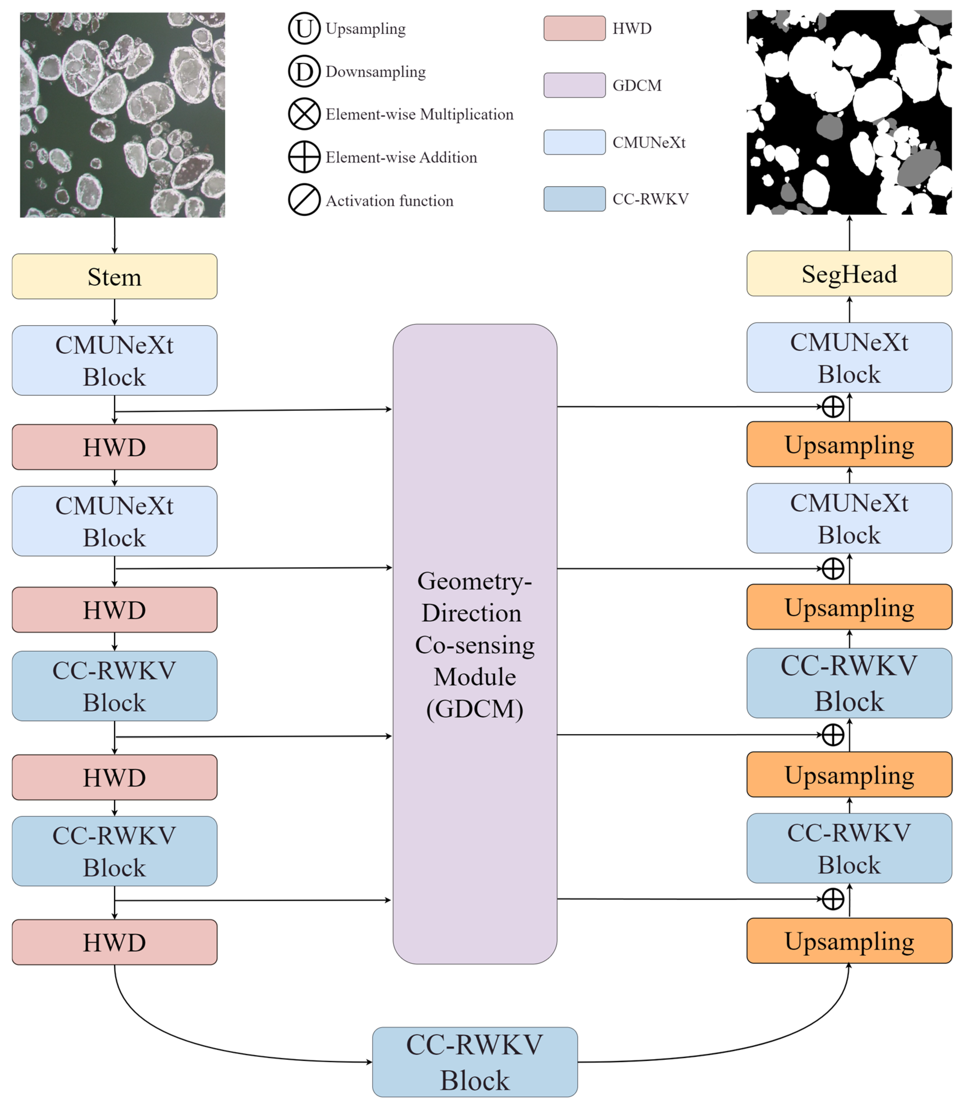
We propose a U-shaped encoder–decoder architecture based on RWKV for river ice segmentation. As illustrated in Figure 1, the shallow network of the encoder embeds CMUNeXt [39] convolutional blocks to accurately capture high-resolution texture details within a limited receptive field. The deep network innovatively introduces the CC-RWKV block, which aims to establish long-range semantic dependencies and enhance the feature representation of river ice through linear sequence modeling and a global-context clustering mechanism. Furthermore, the model employs HWD [40] to replace traditional pooling strategies, effectively mitigating detail loss and feature aliasing. The decoder structure is strictly symmetrical to the encoder, achieving precise feature restoration. To overcome the limitations of conventional convolutions in representing irregularly shaped river ice targets, we design the GDCM. By aggregating multi-scale features and combining adaptive geometric correction with directional polarization enhancement, this module achieves comprehensive geometry-direction co-awareness.

2.2. Context Clustering RWKV

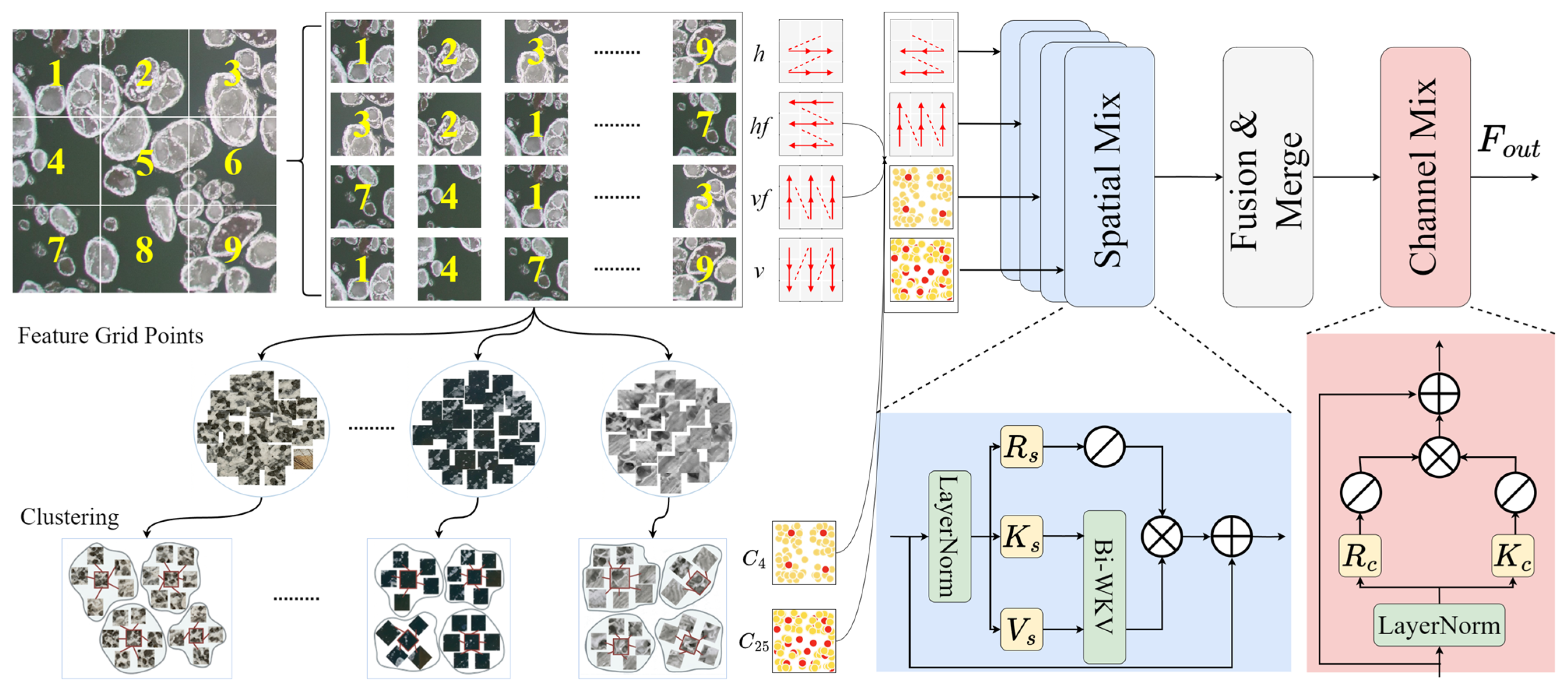
Due to the highly complex and non-directional spatial distribution of river ice, conventional RWKV models tend to destroy local 2D spatial neighborhood relationships when flattening 2D images into 1D sequences. Moreover, fixed scanning paths can easily introduce directional biases, leading to insufficient extraction accuracy for small, irregularly edged obstacles or broken ice. To address this, we propose the CC-RWKV Block. This module utilizes multidirectional visual scanning to obtain a global receptive field, thereby eliminating directional bias. Simultaneously, it introduces a dual-scale context clustering mechanism that treats pixels as an unordered point set for semantic aggregation. Consequently, it achieves adaptive feature extraction and refined reconstruction of complex terrain morphologies while maintaining linear computational complexity.

As shown in Figure 2, for the input features $X\in {\mathbb{R}}^{C\times H\times W}$, we first divide them along the channel dimension into four symmetrical sub-branches $X_{scan}=\{x_h,x_{hf},x_v,x_{vf}\}$, corresponding to horizontal (H), horizontal flip (HF), vertical (V), and vertical flip (VF) scanning paths, respectively. To break the isolation of the local receptive field caused by purely linear sequences, an adaptive pixel shift operator $q_{shift}$ is applied to each branch prior to serialization, forcing adjacent pixels to interact in the sequence dimension. The four multidirectional intersecting scanning paths ensure that the model possesses directional unbiasedness when capturing long-range dependencies. The aforementioned process can be expressed formally:

$$x_i=Serialize(Shift(X_i,q_{shift})),i\in \{h,hf,v,vf\}$$

(1)

Next, to compensate for the inadequate perception of local non-rigid deformations by linear scanning, the pixel-wise average features $X_{avg}$ of the four scanning branches are first extracted as a spatial prior. Subsequently, the features $X_{avg}$ are flattened into an unordered data point set $P\in {\mathbb{R}}^{C^{\prime }\times H\times W}$, and coarse-grained ($k=4$) and fine-grained ($k=25$) context clustering are executed in parallel within the feature space. For the clustering process at any granularity, the model calculates the cosine similarity between local pixel points and $k$ center points, performing dynamic allocation. Within the same cluster including $m$ points, the features of all points $p_i$ are dynamically weighted and aggregated to the center feature $g$ based on similarity $s_i$; then, they are redistributed to each point in the cluster according to similarity for feature updating. This process can be formulated as follows:

$$X_{scan}=Mean(X_{scan})$$

(2)

$$g={\displaystyle \frac{1}{T}}\left(v_c+{\displaystyle \sum _{i=1}^m\sigma }(\alpha s_i+\beta )\ast p_i\right)$$

(3)

$$p_i^{\prime }=p_i+FC(\sigma (\alpha s_i+\beta )\ast g)$$

(4)

where $v_c$ denotes the center of the value space, $\alpha$ and $\beta$ are learnable parameters, $\sigma$ is the Sigmoid activation function used to rescale the weights, and $T=1+{\displaystyle \sum _{i=1}^m\sigma }(\alpha s_i+\beta )$ is a normalization factor.

This process transcends the limitations of fixed grid receptive fields, accomplishing global interaction through semantic consistency. Restoring all updated point sets $P_k^{\prime }=\{p_1^{\prime },p_2^{\prime },\dots ,p_N^{\prime }\}$ at a specific granularity back into a spatial sequence forms a highly adaptive clustered feature branch $F_{ck}$. For both coarse-grained ($k=4$) and fine-grained ($k=25$) clustering, the above aggregation process can be uniformly expressed as:

$$F_{ck}=Reshape(P_k^{\prime }),k\in \{4,25\}$$

(5)

Subsequently, the model constructs a unified candidate pool $\Omega =\{x_h,x_{hf},x_v,x_{vf},F_{c4},F_{c25}\}$ containing four directional scanning branches and two clustering branches. Through a branch selection mechanism, the four core branches with the highest spatial diversity and global vision are filtered from the pool $\Omega$ to form the optimal set $\mathcal{Z}\subset \Omega$. The selected sequences $z_j\in \mathcal{Z}$ then independently enter the linear RWKV spatial mix block (Spatial Mix) for global-context modeling. Following this, the outputs of the four branches that have undergone long-range modeling are restored to the 2D space and concatenated along the channel dimension to obtain $Y_{cat}$. To promote the interweaving of information between scanning directions and clustering granularities, the model applies channel shuffling and spatial attention to $Y_{cat}$ to generate fused features $Y_{fuse}$ with global awareness. The above process is expressed as follows:

$$Y_j=z_j+Spatial-Mix(z_j)$$

(6)

$$Y_{cat}=Concat(Y_1,Y_2,Y_3,Y_4)$$

(7)

$$Y_{fuse}=SpatialAttention(ChanneShuffle(Y_{cat}))$$

(8)

Finally, the fused features $Y_{fuse}$ are reduced in dimensionality and input into the RWKV channel mix block (Channel Mix) to perform feature fusion in the channel dimension. Combined with residual connections, the process of obtaining the final output features $F_{out}$ is expressed as follows:

$$F_{out}=Conv(Y_{fuse})+Channel-Mix(Conv(Y_{fuse}))$$

(9)

The overall procedure of the proposed CC-RWKV is summarized in Algorithm 1.

Algorithm 1 Procedure of the CC-RWKV Block
Require: Feature map $x\in {\mathbb{R}}^{B\times C\times H\times W};$ pixel shift $q_{\mathrm{shift}};$ clustering operators ${\mathrm{CC}}_4$ and ${\mathrm{CC}}_{25};$ spatial-mix operators ${\mathrm{SM}}^{(k)};$ spatial attention $\varphi$ channel mix $\mathrm{CM}$
Ensure: Output feature map $F_{\mathrm{out}}\in {\mathbb{R}}^{B\times C\times H\times W}$
1 Let $C_b\leftarrow C/4,\mathcal{D}\leftarrow \{\mathrm{h},\mathrm{hf},\mathrm{v},\mathrm{vf}\};$
2 $(X^{(\mathrm{h})},X^{(\mathrm{hf})},X^{(\mathrm{v})},X^{(\mathrm{vf})})\leftarrow {\mathrm{Split}}_C(x);$
3 For each $i\in \mathcal{D}$ do
4    $t_i\leftarrow {\mathrm{Orient}}_i(X^{(i)})$	//reverse scan alignment
5    $s_i\leftarrow {\mathrm{Serialize}}_i(\mathrm{Shift}(t_i,q_{\mathrm{shift}}))$
6    ${\tilde{x}}^{(i)}\leftarrow {\mathrm{Orient}}_i^{-1}({\mathrm{Unvec}}_i(s_i))$
7 End for
8 $X_{\mathrm{avg}}\leftarrow {\displaystyle \frac{1}{4}}{\displaystyle \sum _{i\in \mathcal{D}}{\tilde{x}}^{(i)}};$
9 $F_{c4}\leftarrow {\mathrm{CC}}_4(X_{\mathrm{avg}});F_{c25}\leftarrow {\mathrm{CC}}_{25}(X_{\mathrm{avg}});$
10 $\Omega \leftarrow \{{\tilde{x}}^{(\mathrm{h})},{\tilde{x}}^{(\mathrm{hf})},{\tilde{x}}^{(\mathrm{v})},{\tilde{x}}^{(\mathrm{vf})},F_{c4},F_{c25}\};$
11 $\mathcal{Z}\leftarrow \mathrm{SelectBranches}(\Omega ,4);\mathcal{Y}\leftarrow [];$
12 For each branch $z_j\in \mathcal{Z}$ with key $k_j$ do
13    $S_j\leftarrow {\mathrm{Vec}}_{k_j}(z_j)$	//RWKV spatial mix
14    $Y_j\leftarrow {\mathrm{Unvec}}_{k_j} \left(S_j+{\mathrm{SM}}^{(k_j)}(S_j)\right)$
15    Append $Y_j$ to $\mathcal{Y}$
16 End for
17 $Y_{\mathrm{cat}}\leftarrow {\mathrm{Concat}}_C(\mathcal{Y});$
18 $Y_{\mathrm{fuse}}\leftarrow \varphi \left(\mathrm{ChannelShuffle}(Y_{\mathrm{cat}},4)\right);$
19 $U\leftarrow {\mathrm{Conv}}_{1\times 1}(Y_{\mathrm{fuse}})$	//RWKV channel mix
20 $F_{\mathrm{out}}\leftarrow U+\mathrm{CM}(U);$
21 Return $F_{\mathrm{out}}$

2.3. Geometry-Direction Co-Sensing Module

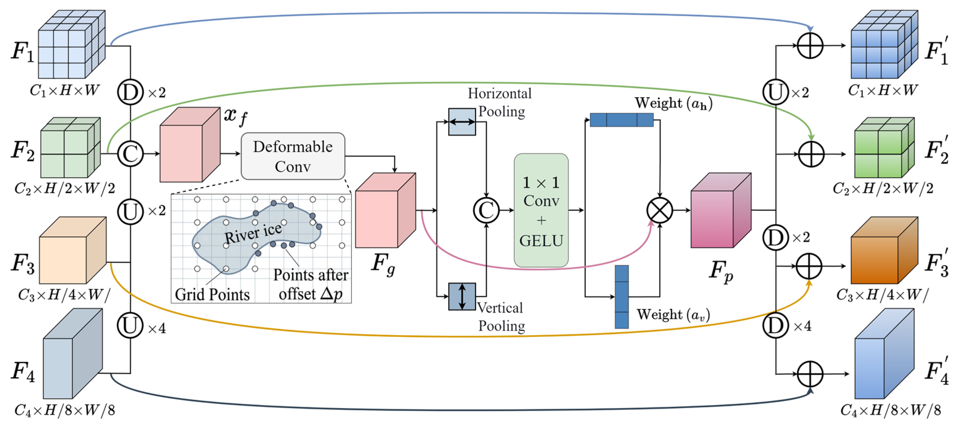
To overcome the shortcomings of conventional convolutions in representing irregularly shaped river ice targets, we designed the GDCM. As illustrated in Figure 3, multi-scale features $F_i(i=1,2,3,4)$ are first mapped to a unified spatial scale through resampling and channel adjustment, and are then aggregated to form fused features $F_f$. Next, deformable convolutions are utilized to learn offsets $\Delta p_k$, enabling the sampling points to conform to the geometric contours of the river ice. For a given position $p_0$ on the output feature map, the corresponding geometric output feature $F_g$ is calculated using the following formula:

$$F_g(p_0)={\displaystyle \sum _{k=1}^K{w}_k}\cdot F_f(p_0+p_k+\Delta p_k)\cdot \Delta m_k$$

(10)

where $p_k$ denotes the standard sampling offset, $\Delta p_k$ represents the adaptive geometric offset, and $\Delta m_k$ signifies the modulation factor for adjusting sampling weights.

Building upon this, we introduce a polarized feature-refinement mechanism to deeply reconstruct the output geometric features. It first compresses spatial contexts along the width and height dimensions via Axial Pooling to generate vector features with directional awareness. Subsequently, operations such as dimensional concatenation and convolutional transformation are utilized to enhance cross-dimensional nonlinear correlations. Finally, the attention weights of height $a_h$ and width $a_w$ are calculated through a weight redistribution branch, and the original features are weighted and modulated using element-wise broadcast multiplication to obtain the polarization-superimposed features $F_p$. Through this polarization processing, background noise in non-river regions is significantly suppressed, while the linear feature signals conforming to the river’s flow direction achieve precise spatial reconstruction. The above process can be expressed as:

$$F_p=F_g\otimes \sigma (Con{v}_h(a_h))\otimes \sigma (Con{v}_w(a_w))$$

(11)

where $\sigma$ denotes the GELU activation function, and $\otimes$ represents the element-wise product. Ultimately, the final enhanced multi-scale features $F_i^{\prime }(i=1,2,3,4)$ are obtained through operations such as resampling and residual connections.

2.4. Haar Wavelet Downsampling

Traditional downsampling operations typically reduce the size of feature maps by discarding pixels or through local aggregation. This easily leads to feature aliasing between different ice categories and results in the loss of detailed features. Therefore, we introduce HWD into the river ice segmentation task.

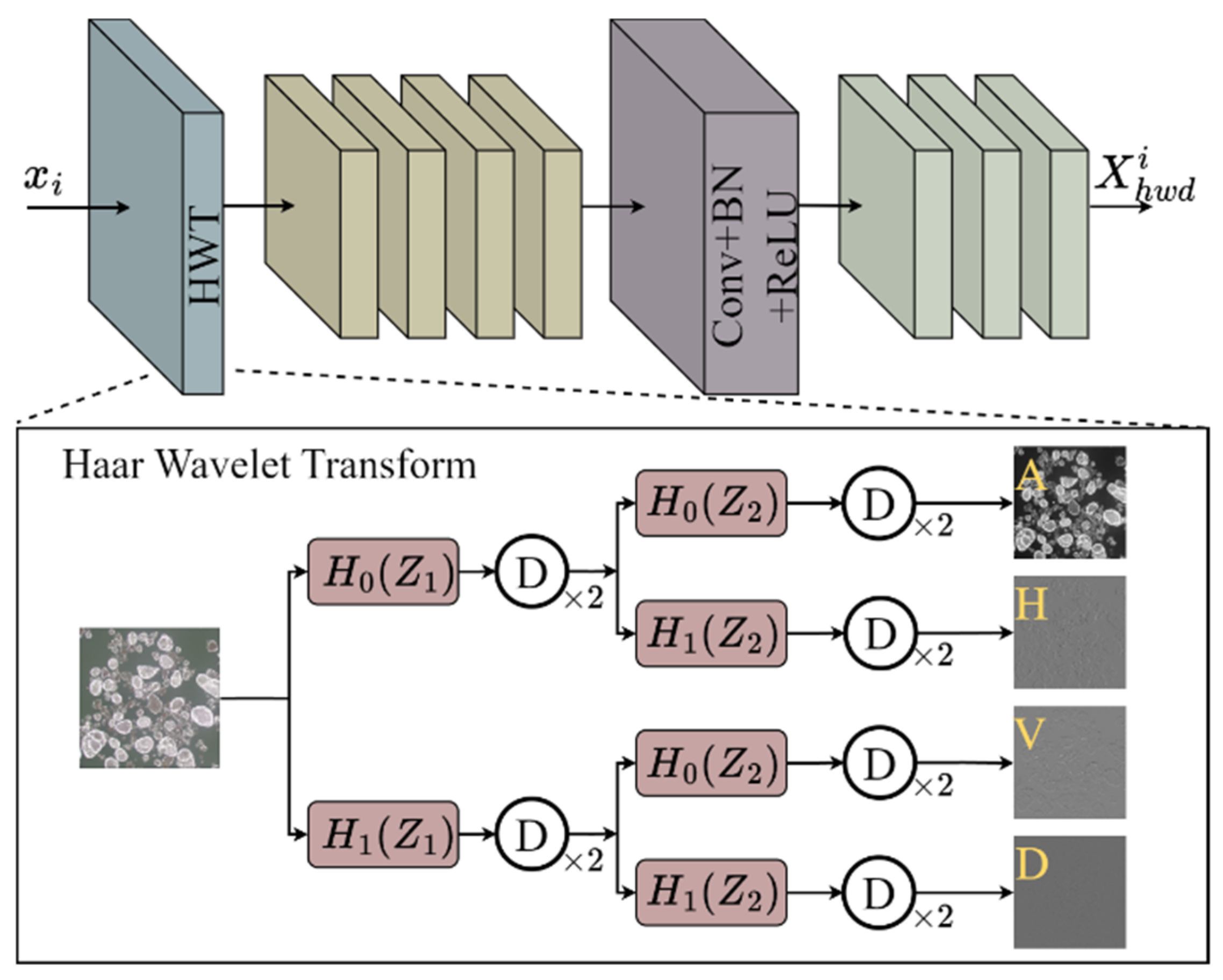
Specifically, we integrate the Haar wavelet transform into the downsampling stage of the model, replacing traditional convolutional downsampling (Figure 4). Regarding the input feature representation $F_i(i=1,2,3,4)$, the HWD module utilizes four Haar wavelet operators to perform convolutions with the input features, decomposing them into four frequency sub-bands: one low-frequency approximation map and three high-frequency detail maps corresponding to the horizontal, vertical, and diagonal directions. Finally, the HWD module concatenates the features of these four branches along the channel dimension and applies a $1\times 1$ convolutional layer to adjust the number of channels. The aforementioned process can be expressed as follows:

$$X_{LL}=F_i\otimes f_{LL},X_{LH}=F_i\otimes f_{LH},X_{HL}=F_i\otimes f_{HL},X_{HH}=F_i\otimes f_{HH}$$

(12)

$$F_i^{hwd}=\sigma (BN(Con{v}_{1\times 1}(Concat(X_{LL},X_{LH},X_{HL},X_{HH}))))$$

(13)

where $f_{LL}=\left[\begin{array}{cc}1& 1\\ 1& 1\end{array}\right],f_{LH}=\left[\begin{array}{cc}-1& -1\\ 1& 1\end{array}\right],f_{HL}=\left[\begin{array}{cc}-1& 1\\ -1& 1\end{array}\right],f_{HH}=\left[\begin{array}{cc}1& -1\\ -1& 1\end{array}\right]$ represent Haar wavelet operators, and $\otimes$ denotes the convolution operation.

2.5. Loss Function

To overcome the class imbalance problem in river ice segmentation tasks and accurately extract the geometric edge details of ice blocks, this study constructed a composite loss function ${\mathcal{L}}_{total}$. This function is a weighted combination of Binary Cross-Entropy (BCE) loss ${\mathcal{L}}_{BCE}$ and Dice loss ${\mathcal{L}}_{Dice}$. The BCE loss ${\mathcal{L}}_{BCE}$ evaluates the pixel-wise difference between the predicted probabilities and the ground-truth (GT) labels, ensuring smoothness at the pixel level. Simultaneously, the Dice loss ${\mathcal{L}}_{Dice}$ measures the degree of overlap between the predicted and GT regions, enhancing the model’s ability to perceive small targets. The final overall loss function is defined as the linear weighted sum of the two. The aforementioned process is expressed as follows:

$${\mathcal{L}}_{BCE}=-{\displaystyle \frac{1}{N}}{\displaystyle \sum _{i=1}^N[y_i}\log ({\widehat{y}}_i)+(1-y_i)\log (1-{\widehat{y}}_i)]$$

(14)

$${\mathcal{L}}_{Dice}=1-{\displaystyle \frac{2{\displaystyle \sum _{i=1}^N{y}_i}{\widehat{y}}_i+ϵ}{{\displaystyle {\displaystyle \sum _{i=1}^N}{y}_i}+{\displaystyle {\displaystyle \sum _{i=1}^N}{\widehat{y}}_i}+ϵ}}$$

(15)

$${\mathcal{L}}_{total}={\lambda }_1{\mathcal{L}}_{BCE}+{\lambda }_2{\mathcal{L}}_{Dice}$$

(16)

where $N$ denotes the total number of pixels, $y_i\in \{0,1\}$ represents the ground-truth label of the $i$-th pixel, and ${\widehat{y}}_i$ is the model’s predicted probability that the pixel belongs to an ice body; $ϵ$ is a smoothing factor.

3. Experimental Results and Analysis

3.1. Dataset

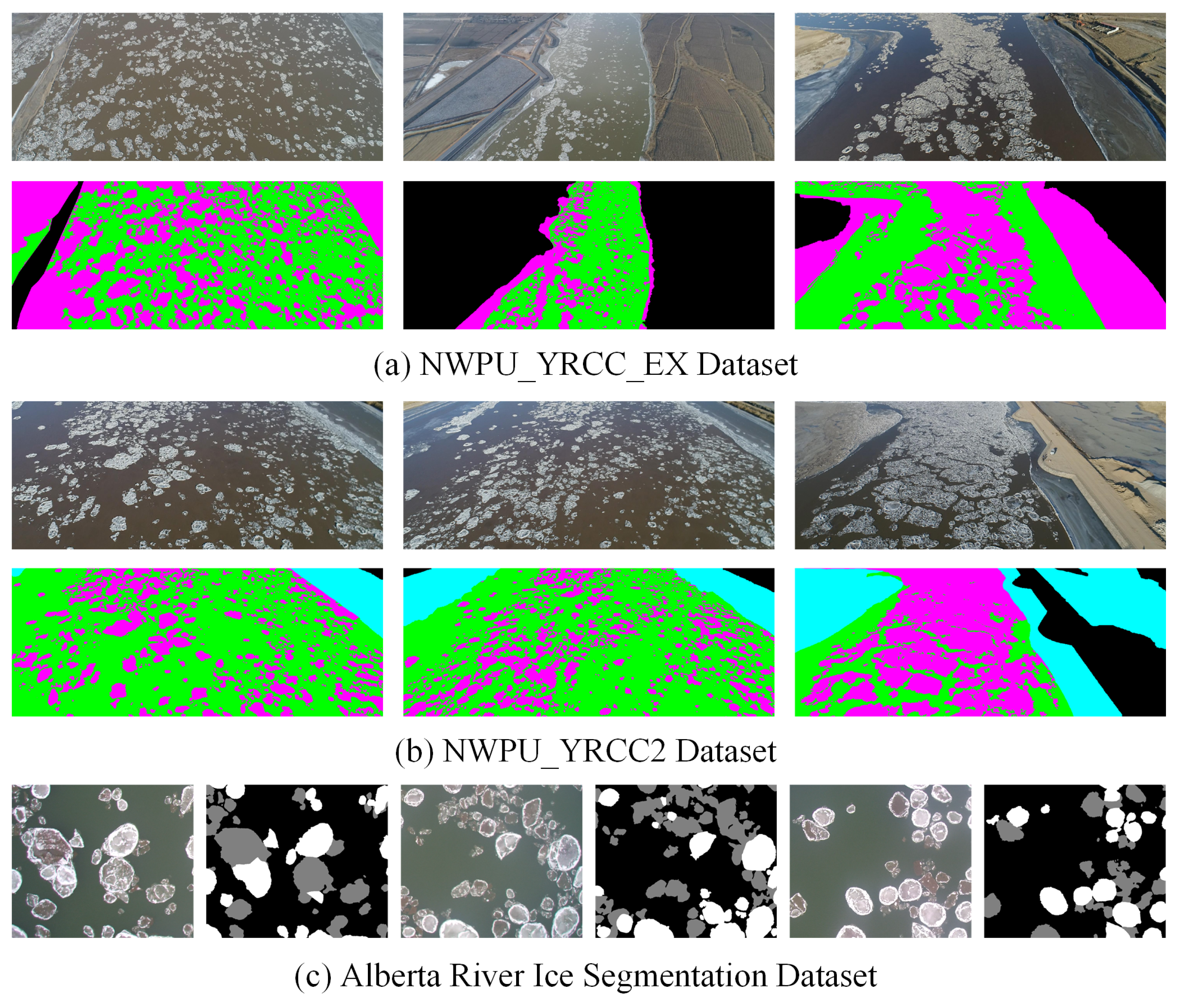
This subsection introduces three challenging public datasets used for river ice semantic segmentation, with representative samples from each dataset shown in Figure 5.

3.1.1. NWPU_YRCC_EX Dataset

The NWPU_YRCC_EX dataset contains 887 images of 1600 × 840 pixels, which are derived from UAV imagery captured in the Ningxia-Inner Mongolia section of the Yellow River from November 2015 to March 2019. It includes ice, water, and shore. Specifically, the dataset is partitioned into 524 training, 180 validation, and 183 testing images.

3.1.2. NWPU_YRCC2 Dataset

The NWPU_YRCC2 dataset comprises 1525 annotated 1600 × 640-pixel images. These samples were derived from drone-acquired footage over the Ningxia-Inner Mongolia reach of the Yellow River between November 2015 and March 2019. This dataset contains four categories: shore, water, shore ice, and drift ice; ultimately, 915 images were utilized for training, 305 for validation, and 305 for testing.

3.1.3. Alberta River Ice Segmentation Dataset

The Alberta River Ice Segmentation Dataset was collected by UAVs and bridge-mounted cameras on two rivers in Alberta, Canada, during the winters of 2016 and 2017. This dataset contains three categories: drift ice, anchor ice, and water. The vast majority of images have a dimension of 1281 × 1081 pixels, and it contains only 50 manually annotated original images. To strictly prevent spatial data leakage between training and evaluation phases, these 50 original images were first partitioned at the image level into independent training, validation, and testing sets according to a 6:2:2 ratio. Following the strategy of Zhang et al. [26], random cropping to a size of 800 × 320 pixels was subsequently performed independently within each subset, ultimately yielding 198 fully labeled sub-image samples.

3.2. Experimental Setup

3.2.1. Implementation Details

All experiments were implemented based on the PyTorch 1.9.1, and the experimental platform was a server equipped with dual Intel Xeon Gold 5320 processors and a NVIDIA A800 GPU (80GB VRAM). To ensure the fairness of the experimental comparison, all networks adopted the AdamW optimizer for model training, with the initial learning rate set to 5 × 10⁴ and the weight decay coefficient set to 0.01. A polynomial decay strategy was chosen for the learning rate scheduling strategy; the total training epochs for the model were 200, and the batch size was set to 16.

3.2.2. Evaluation Metrics

In this study, we adopted Intersection over Union (IoU) and mIoU as quantitative evaluation accuracy metrics. The formulas are as follows:

$$IoU={\displaystyle \frac{TP}{TP+FP+FN}}$$

(17)

$$mIoU={\displaystyle \frac{1}{k}}{\displaystyle \sum _{i=1}^{k}I}o{U}_i$$

(18)

where $TP$, $FP$, and $FN$ denote the numbers of true-positive, false-positive, and false-negative predictions, respectively; $k$ and $i$ denote the total number of semantic classes and the class index, respectively.

In addition, we incorporated computational efficiency metrics, including inference speed and model parameters. Inference speed is quantified by FPS, which reflects the model’s throughput during real-time inference. Model size is evaluated by the total number of learnable parameters, which indicates architectural complexity.

3.3. Algorithms for the Comparative Evaluation

To comprehensively verify the performance advantages of the proposed model in the river ice semantic segmentation task, this study selected 10 representative methods from CNN architectures, Transformer architectures, RWKV architectures and dedicated river ice extraction models, to conduct qualitative and quantitative comparative experiments.

Among them, PIDNet-L [41] simultaneously retains details and context information through a parallel branch design, performing excellently in real-time semantic segmentation tasks, and serving as a reliable baseline for general segmentation tasks. BiseNet [42] adopts a dual-branch structure to balance accuracy and speed, possessing good generalization ability in complex scene segmentation. ContextNet [43] expands the receptive field through dilated convolutions, which can effectively capture long-range contextual dependencies and is suitable for large-scale remote sensing image segmentation tasks. UNetFormer [44] integrates a U-shaped structure and the Transformer attention mechanism, balancing local details and global-context modeling, and demonstrating powerful performance in remote sensing image segmentation. BuildFormer [45] is optimized for building extraction tasks, possesses outstanding global perception capabilities, and can be effectively transferred to complex terrain recognition tasks such as ice condition segmentation. DA_ViT [46] adaptively focuses on key regions through a dynamic attention mechanism, which can significantly improve segmentation accuracy under complex ice condition scenarios. ICENet [47] is a dedicated network designed for the river ice segmentation task; through an ice condition specific feature extraction module, it possesses a natural advantage in ice condition recognition. ICENet v2 [37] optimized and designed a multi-level feature fusion framework, dual attention modules, and a learnable upsampling strategy based on ICENet, focusing on resolving core difficulties such as the large-scale differences, intra-class heterogeneity, and inter-class homogeneity of river ice. FastICENet [26] optimized the network structure based on ICENet, achieving a balance between accuracy and inference speed, making it suitable for real-time ice condition monitoring scenarios. FastICENet (acc) [26] enhances segmentation accuracy through optimized feature fusion while maintaining computational efficiency. Vision-RWKV [48] employs the RWKV sequence modeling mechanism to capture long-range spatial dependencies with linear complexity, enabling efficient global-context modeling for semantic segmentation. U-RWKV [49] integrates RWKV blocks into a U-shaped architecture, combining global contextual information with multi-scale feature representations for semantic segmentation.

3.4. Results and Analysis

3.4.1. Results on the NWPU_YRCC_EX Dataset

As shown in

Table 1. Comparison with SOTA methods on the NWPU_YRCC_EX dataset.

Methods	IoU (%)			mIoU (%)	Speed	Parameters (k)
	Ice	Water	Other
PIDNet-L	92.69	88.64	92.05	91.25	53.75	37,306
BiseNet	91.22	87.61	90.34	89.72	44.75	14,090
ContextNet	92.63	87.12	85.01	87.16	101.11	874
UNetFormer	90.43	84.88	71.63	82.31	80.90	11,725
BuildFormer	92.61	89.18	78.46	86.75	66.84	40,519
DA_ViT	93.26	89.02	84.78	89.02	76.44	19,301
ICENet	91.58	84.89	88.25	88.11	-	-
ICENetv2	90.91	86.10	90.37	88.51	-	-
FastICENet	92.10	88.12	92.08	90.77	94.84	969
FastICENet (acc)	92.90	89.65	93.02	91.86	44.50	14,090
Vision-RWKV	91.34	88.42	90.69	90.15	21.36	6213
U-RWKV	92.05	86.11	90.28	89.48	13.58	2972
IceRWKV (ours)	94.65	90.27	95.31	93.41	37.19	2919

, the proposed IceRWKV model achieves SOTA performance on all evaluation metrics. When compared with the second-best baseline FastICENet, IceRWKV improves the mIoU from 91.86% to 93.41% and attains a segmentation accuracy of 94.65% for the ice class. Other competitive architectures, including Vision-RWKV and U-RWKV, obtain mIoUs of 90.15% and 89.48%, respectively, both of which are surpassed by our approach. Furthermore, against lightweight real-time CNN models such as ContextNet, IceRWKV retains a very compact parameter size of only 2.919 M, while boosting the mIoU substantially from 87.16% to 93.41%.

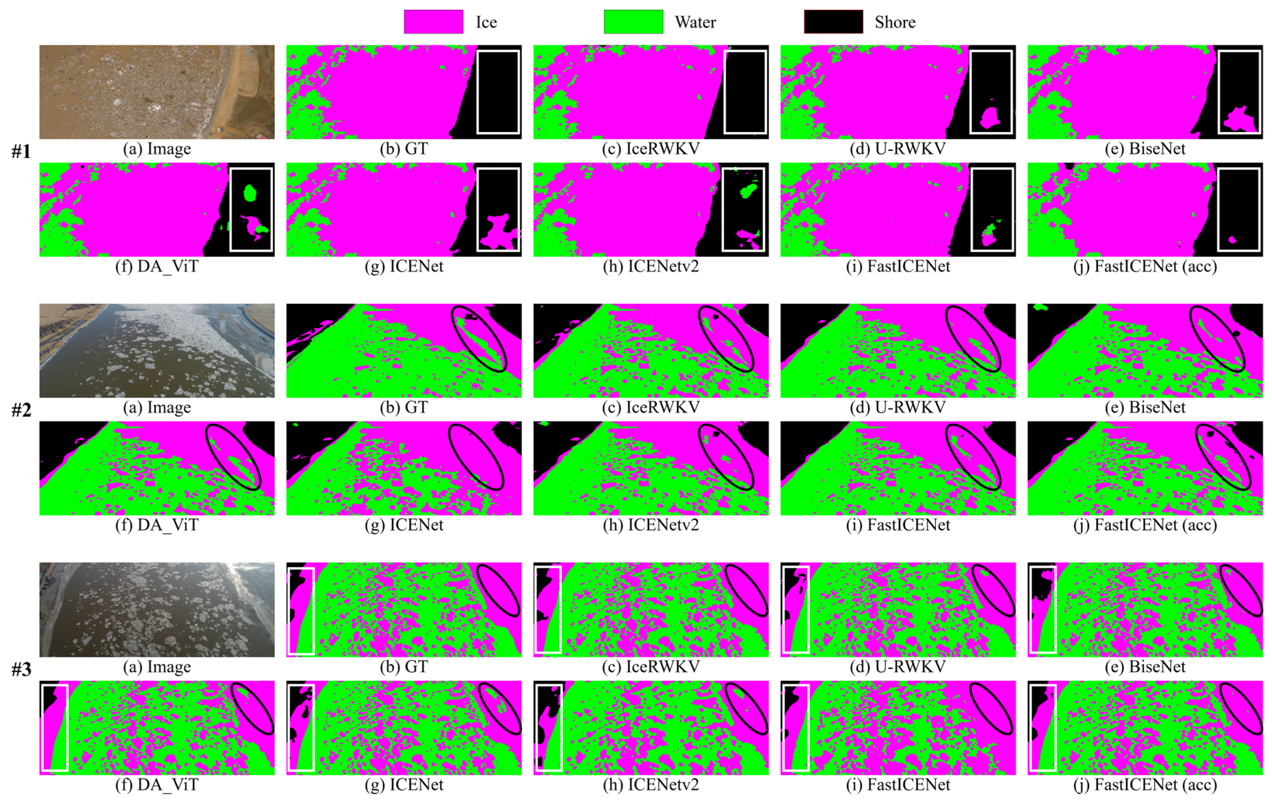
We also visualized the segmentation results of representative comparison networks and our proposed method on the NWPU_YRCC_EX dataset. As shown in Figure 6, regarding the complex background in scene #1 (white solid-line box), the polarized feature-refinement mechanism embedded in the GDCM effectively filters out noise interference from non-river regions, significantly reducing the false detection rate. Meanwhile, addressing the disadvantage of the FastICENet series, which is prone to generating prediction cavities in dense broken ice areas, the CC-RWKV block substantially enhances the network’s ability to efficiently identify and reconstruct minute, dense features, thereby enabling it to clearly and completely segment the small water bodies and shores interspersed within the river ice (the solid black elliptical regions in scenes #2 and #3). In addition, observing the solid white box in scene #3 reveals that, compared to the inadequate edge segmentation sharpness of Transformer architectures like DA_ViT, IceRWKV demonstrates the best morphological fidelity in near-shore areas. This is primarily attributed to the adaptive geometric correction strategy of the GDCM, which realizes precise adaptive fitting for irregular shorelines and ice body contours.

3.4.2. Results on the NWPU_YRCC2 Dataset

As shown in

Table 2. Comparison with SOTA methods on the NWPU_YRCC2 dataset.

Methods	IoU (%)				mIoU (%)	Speed	Parameters (k)
	Drift Ice	Shore Ice	Water	Other
PIDNet-L	79.78	81.26	87.71	76.15	81.22	60.35	37,306
BiseNet	72.62	84.03	87.28	76.44	80.09	59.85	14,090
ContextNet	74.35	74.93	83.89	78.15	77.83	116.63	874
UNetFormer	80.41	74.16	86.76	77.52	79.71	84.46	11,725
BuildFormer	82.59	78.57	90.02	74.86	81.51	67.58	40,519
DA_ViT	84.28	82.29	90.67	79.55	84.20	76.36	19,301
ICENet	74.45	82.80	87.87	77.05	80.54	-	-
ICENetv2	81.13	81.58	90.48	80.55	83.44	-	-
FastICENet	79.34	80.83	87.25	75.75	80.79	108.78	969
FastICENet (acc)	81.97	80.40	89.71	79.80	81.87	51.13	14,090
Vision-RWKV	81.14	80.65	89.26	79.47	82.63	32.76	6213
U-RWKV	79.83	78.49	88.61	77.23	81.04	46.82	2972
IceRWKV (ours)	86.21	85.37	92.11	83.47	86.79	42.34	2919

, IceRWKV further demonstrates exceptional generalization capability on the NWPU_YRCC2 dataset, lifting the mIoU from 84.20% (achieved by the second-best DA_ViT) to 86.79%. In comparison, other RWKV-based models, Vision-RWKV and U-RWKV, yield lower mIoU scores of 82.63% and 81.04%, respectively. Particularly in the shore ice class, IceRWKV’s IoU rises substantially from 82.29% (DA_ViT) to 85.37%, outperforming all other networks by a notable margin.

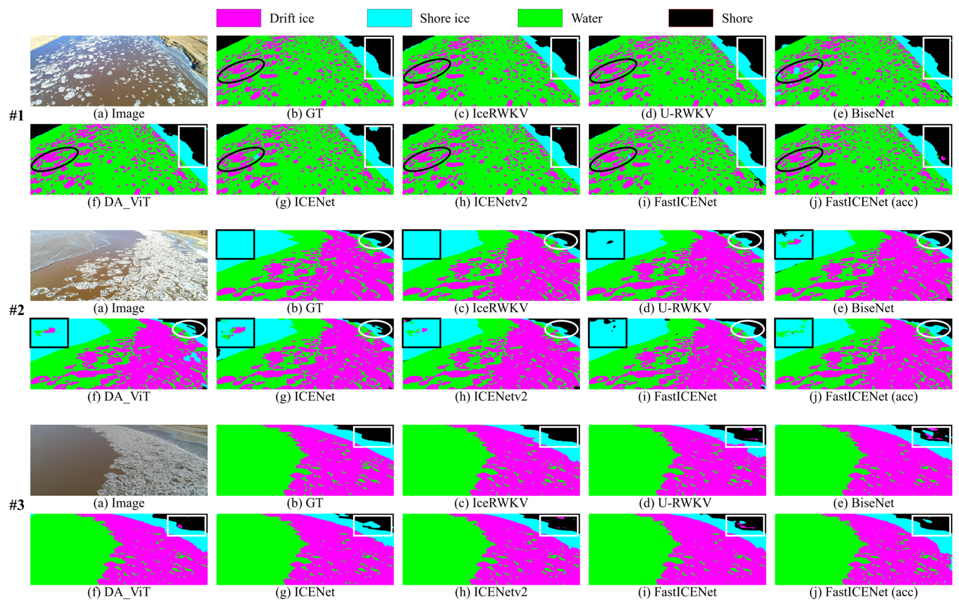
To further explore the effectiveness of the proposed modules, visual comparison results of related networks are presented in Figure 7. As shown in the solid black circle regions of scenes #1 and #2, when facing the easily confused boundaries among ice, water, and shore, the GDCM endows the network with powerful adaptive geometric deformation modeling capabilities, enabling it to precisely conform to highly irregular natural shorelines, thereby substantially reducing category misclassifications and feature omissions commonly found in other networks. On the other hand, the solid white circles in scenes #2 and #3 further confirm the GDCM’s enhanced perception of the river’s longitudinal flow characteristics. Traditional convolutional or self-attention networks are prone to context information loss and prediction fractures at such narrow and complex geographical edges. Benefiting from the module’s “geometry-direction” dual collaborative sensing mechanism, IceRWKV not only effectively extracts flow prior information with strong directionality, but also finely captures the elongated shore ice edges tightly distributed along the coastline.

3.4.3. Results on the Alberta River Ice Segmentation Dataset

As shown in

Table 3. Comparison with SOTA methods on the Alberta River Ice Segmentation dataset.

Methods	IoU (%)			mIoU (%)	Speed	Parameters (k)
	Water	Anchor Ice	Drift Ice
PIDNet-L	95.87	72.66	77.86	82.10	90.58	37,306
BiseNet	95.09	72.03	77.81	81.24	74.81	14,090
ContextNet	94.90	68.60	72.44	78.64	172.83	874
UNetFormer	92.80	69.06	51.82	71.23	130.64	11,725
BuildFormer	94.31	75.35	57.45	75.70	39.24	40,519
DA_ViT	93.78	70.46	55.87	73.37	52.18	19,301
FastICENet	95.57	72.28	77.46	81.77	159.82	969
FastICENet (acc)	95.96	73.88	78.33	82.34	73.50	14,090
Vision-RWKV	94.61	71.85	76.33	80.93	39.42	6213
U-RWKV	93.92	70.16	74.24	79.44	57.36	2972
IceRWKV (ours)	96.57	77.01	78.59	84.06	50.47	2919

, IceRWKV similarly exhibits the best overall segmentation performance on the cross-regional Alberta River Ice Segmentation Dataset. Compared to the strong baseline network FastICENet (acc), the mIoU of our model improves from 82.34% to 84.06%. Meanwhile, other RWKV-based baselines, Vision-RWKV and U-RWKV, achieve lower mIoU scores of 80.93% and 79.44%, respectively. Particularly in the anchor ice category, which is easily confused with the background and other ice types, the IoU of IceRWKV increases significantly from 73.88% (FastICENet (acc)) to 77.01%, further validating the model’s fine-grained feature mining capability in complex scenes.

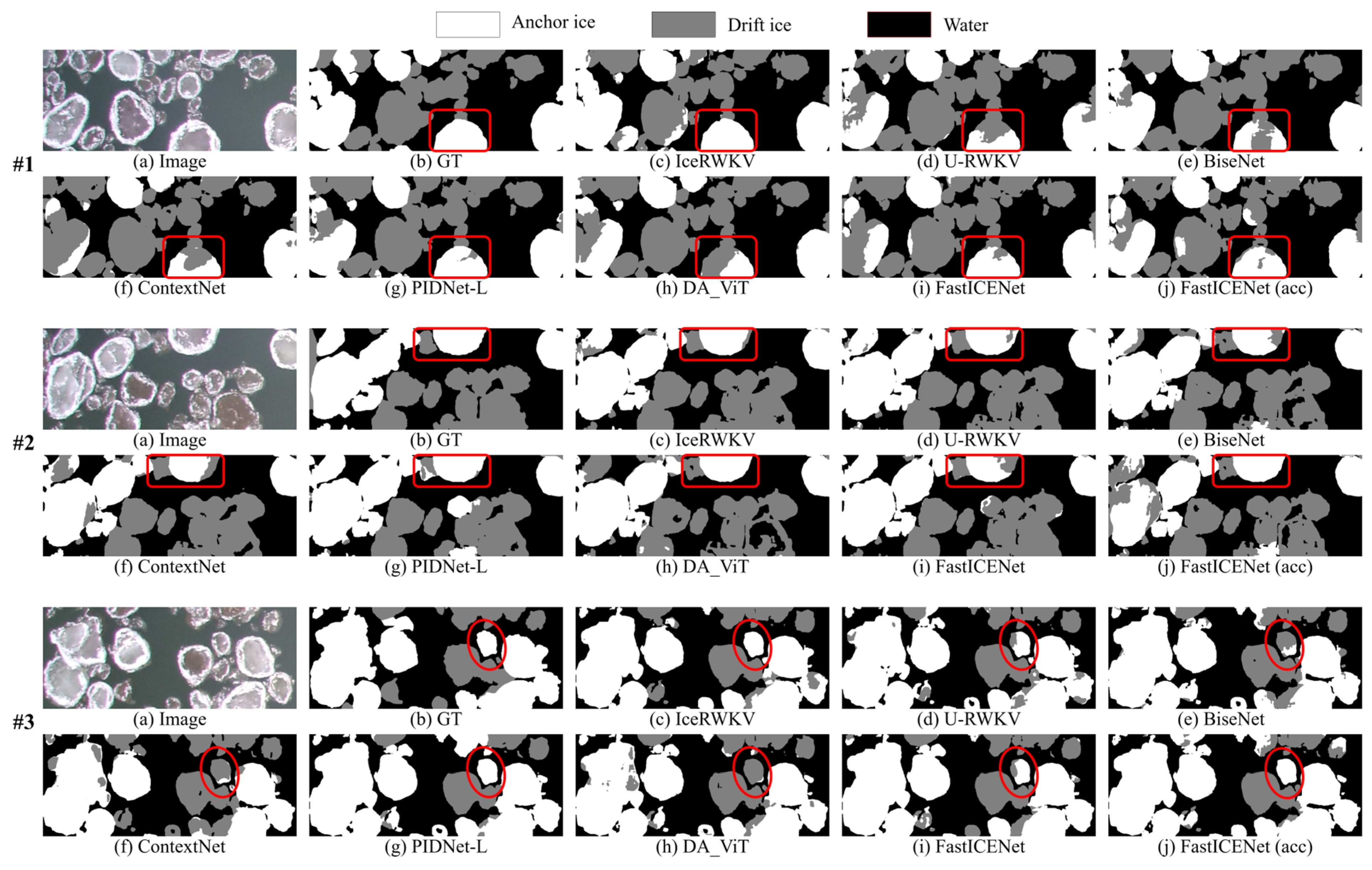
To intuitively demonstrate the detail reconstruction advantages of the proposed method, Figure 8 compares the qualitative visualization results of IceRWKV with networks such as PIDNet-L, BiseNet, and ContextNet. Focusing on the solid red boxes in scenes #1 and #2, it can be observed that conventional networks (e.g., PIDNet-L and ContextNet) easily lose minute target information during spatial feature dimensionality reduction. In contrast, our model, benefiting from the introduced HWD strategy, successfully retains more complete small-scale ice body details through efficient information transfer in the frequency domain, effectively overcoming the feature attenuation and disappearance of fragmented ice blocks. Moreover, observing the solid red elliptical region in scene #3, densely distributed drift ice and anchor ice often lead to severe boundary blurring and color block adhesion phenomena. Faced with this challenge, under the strong synergy of the global linear sequence context modeling and local detail reconstruction mechanisms, IceRWKV significantly suppresses such visual defects, allowing the contours of broken ice of different types and scales to be presented more clearly, independently, and with high fidelity.

3.5. Ablation Study

To verify the effectiveness of each key module in IceRWKV, this study utilized CMUNeXt as the baseline network to conduct comprehensive ablation experiments on the NWPU_YRCC_EX dataset.

3.5.1. Overall Analysis

As shown in

Table 4. Overall ablation study of the proposed IceRWKV on the NWPU_YRCC_EX dataset.

Models	Baseline	CC-RWKV	GDCM	HWD	IoU (%)			mIoU (%)
					Ice	Water	Other
(a)	√				87.06	85.58	88.72	87.12
(b)	√	√			92.51	88.63	91.41	90.85
(c)	√		√		89.38	87.89	89.01	88.76
(d)	√			√	88.52	86.85	89.53	88.30
(e)	√	√	√		94.08	89.78	92.95	92.27
(f)	√	√		√	93.64	88.35	93.41	91.80
(g)	√		√	√	90.41	87.11	91.43	89.65
(h)	√	√	√	√	94.65	90.27	95.31	93.41

Note: “√” indicates the corresponding module is included in the model.

, after adding the CC-RWKV block alone, the model accuracy improves to 90.85%, indicating that RWKV linear sequence modeling combined with context clustering can effectively establish large-scale spatial dependencies for river ice, substantially enhancing global feature expression capabilities. When only the GDCM is introduced, the model obtains a mIoU of 88.76%, a 1.64 percentage point improvement over the baseline. When only the HWD strategy is applied, the mIoU reaches 88.30%, a 1.18 percentage point improvement over the baseline. This indicates that both geometric direction perception and frequency-domain downsampling can improve river ice detail expression to a certain extent, but the improvement magnitude is limited when used individually. Furthermore, combining CC-RWKV with GDCM or HWD increases the model accuracy to 92.27% and 91.80%, respectively, demonstrating a good complementarity among global-context modeling, local geometric modeling, and frequency-domain information retention. Ultimately, when all three modules act synergistically, the overall mIoU of IceRWKV reaches 93.41%, a cumulative improvement of 6.29 percentage points over the baseline, proving that the three modules can work collaboratively to achieve optimal segmentation performance.

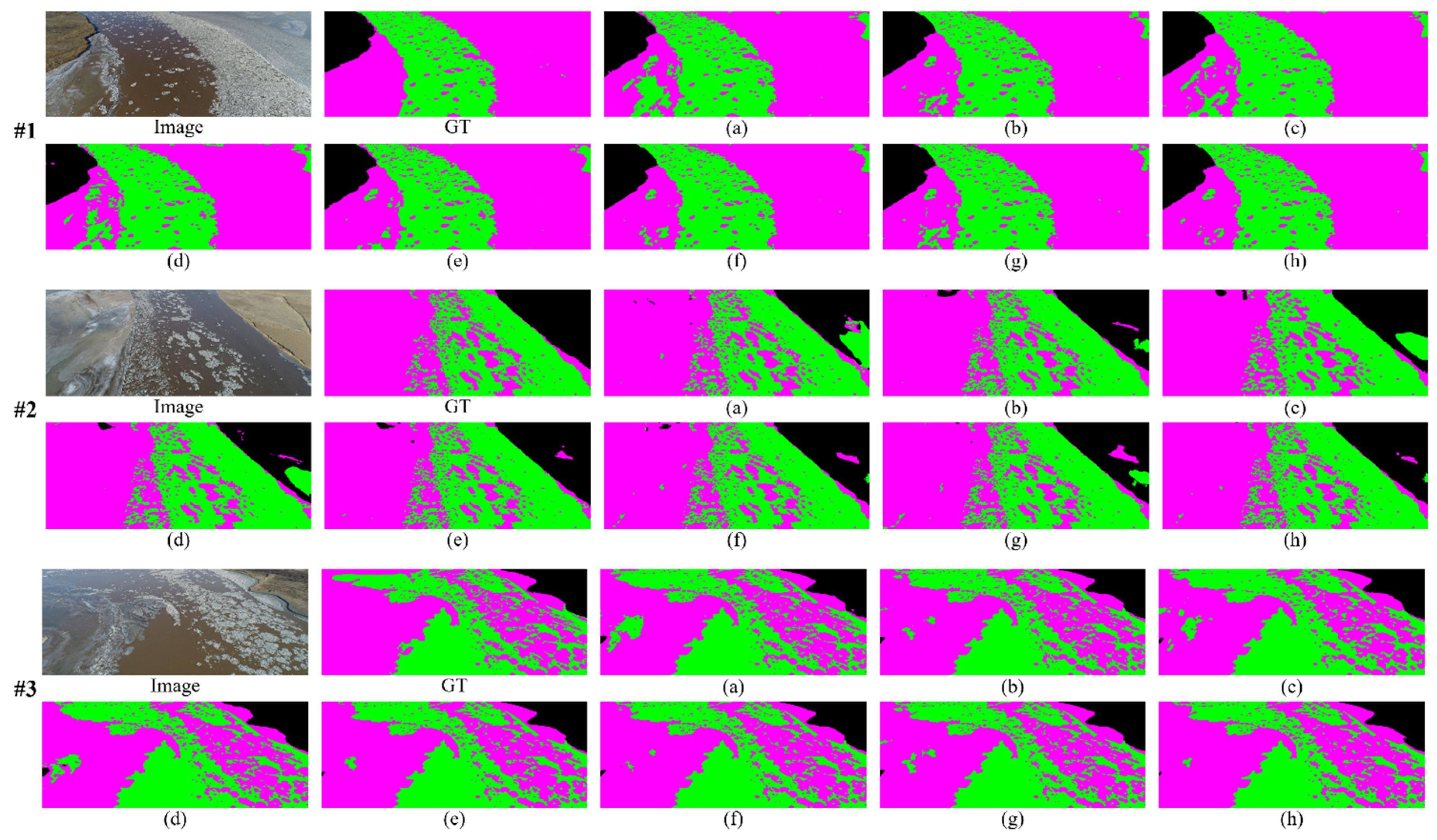
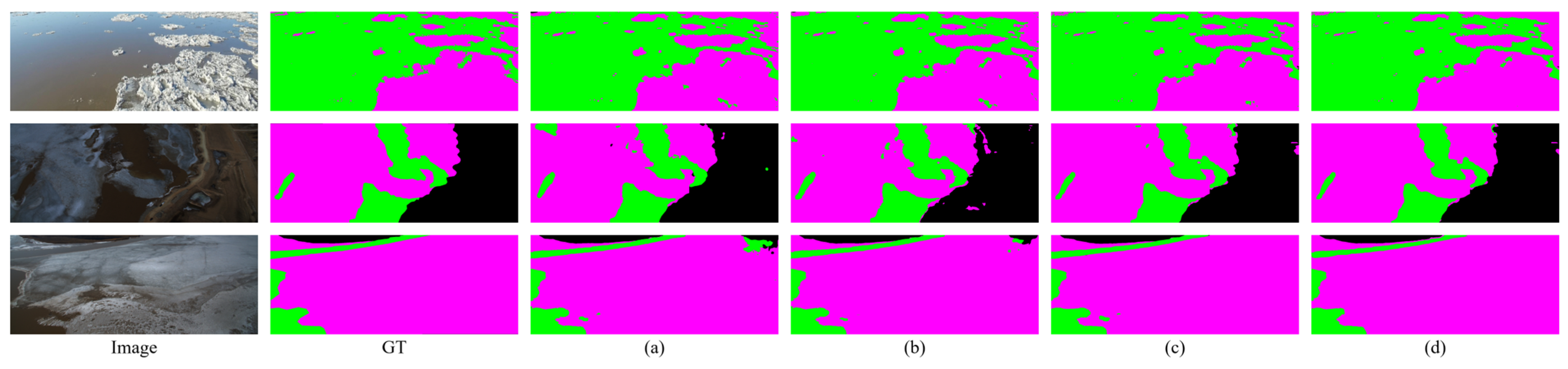
From Figure 9, it can be found that with the gradual addition of the modules, the ice–water boundaries in the prediction results become more continuous, missed detections in broken ice areas are significantly reduced, and the irregular boundaries near the riverbanks can be more accurately restored. In particular, after incorporating CC-RWKV, the prediction fractures appearing within large areas of continuous ice layers essentially disappear. With the further introduction of GDCM, the complex boundaries near the riverbanks fit the true contours more closely. Finally, after adding HWD, small-scale broken ice and elongated ice bands are well preserved, and the overall prediction results exhibit higher consistency with the GT labels.

3.5.2. Effectiveness Analysis of CC-RWKV

As shown in

Table 5. Performance comparison of different RWKV modeling strategies.

Models	Setting	IoU (%)			mIoU (%)
		Ice	Water	Other
(a)	CMUNeXt Block	90.41	87.11	91.43	89.65
(b)	Unidirectional RWKV	92.15	88.24	92.31	90.90
(c)	Quad-WKV	93.05	89.62	94.14	92.27
(d)	CC-RWKV (ours)	94.65	90.27	95.31	93.41

, because conventional convolutions are limited by local receptive fields, the baseline model (a) struggles to fully capture the long-range spatial topological relationships of river ice in vast water bodies, with its mIoU being only 89.65%. Model (b) introduces unidirectional RWKV for 1D sequential modeling, utilizing linear complexity to acquire a global vision, which improves the mIoU to 90.90%, and the critical Ice category IoU increases by 1.74%. However, forcibly flattening a 2D image into a unidirectional 1D sequence disrupts spatial symmetry and introduces directional bias; for targets like river ice that exhibit highly complex spatial orientations, its performance improvement remains limited. To resolve this problem, model (c) adopts a four-directional modeling mechanism, effectively eliminating directional bias by combining forward and backward scans in both horizontal and vertical directions, making feature extraction more balanced and further raising the mIoU to 92.27%. Building on this, the final proposed model (d), CC-RWKV, innovatively introduces a dual-scale context clustering mechanism, completely breaking free from fixed grid constraints. This mechanism treats pixels as an unordered point set for adaptive semantic aggregation, greatly enhancing the anti-tearing extraction capability for discrete broken ice. Ultimately, CC-RWKV achieves the optimal performance leap, with its mIoU reaching 93.41%, and the most challenging Ice category IoU achieving the best performance at 94.65%, fully proving the advancement of this architectural design.

Furthermore, Figure 10 presents a visual segmentation comparison of the ablation models in complex ice–water transition regions. Observing local details reveals that the baseline model (a), which relies solely on local receptive fields, is prone to obvious missed detections within continuous ice layers and exhibits severe boundary adhesion in discrete broken ice areas. After introducing sequential modeling, the model’s continuity in identifying large ice bodies improves somewhat, but models (b) and (c) are still limited by fixed grid scanning paths, resulting in fragmented edges for some irregular broken ice. In contrast, the proposed CC-RWKV, relying on the context clustering mechanism, achieves global interaction of intra-class features across spatial locations. Its segmentation results not only show continuous responses without obvious noise points within large ice areas, but also demonstrate precise boundary fitting capabilities that are highly consistent with the GT labels at strongly non-rigidly deformed broken ice clusters and minute ice cracks.

3.5.3. Effectiveness Analysis of GDCM

To verify the effectiveness of the GDCM proposed in this paper, we compared it with three skip connection methods: Concatenation [50], SDI [51], and SAFM [52], with the experimental results shown in

Table 6. Comparison of different skip connection strategies on the NWPU_YRCC_EX dataset.

Models	Setting	IoU (%)			mIoU (%)
		Ice	Water	Other
(a)	Concatenation	93.64	88.35	93.41	91.80
(b)	SDI	93.88	88.95	94.01	92.28
(c)	SAFM	94.17	89.62	94.85	92.88
(d)	GDCM	94.65	90.27	95.31	93.41

. It can be seen that traditional concatenation fusion obtains a mIoU of 91.80%, adopting SDI improves it to 92.28%, and further adopting SAFM reaches 92.88%. Although these methods can all improve information fusion between the encoder and decoder to some extent, they still easily produce prediction errors in complex boundary regions due to the lack of explicit modeling of river ice geometric morphology and directional information. In contrast, the proposed GDCM achieves the highest mIoU of 93.41%, while the Ice category IoU reaches 94.65% and the Water category reaches 90.27%, all outperforming other fusion strategies. This demonstrates that the GDCM utilizes deformable convolutions to achieve adaptive geometric modeling for irregular ice contours, and combines directional polarized features to further enhance continuous structural expression along the river flow direction; therefore, it can more accurately distinguish between ice bodies, water bodies, and shore areas.

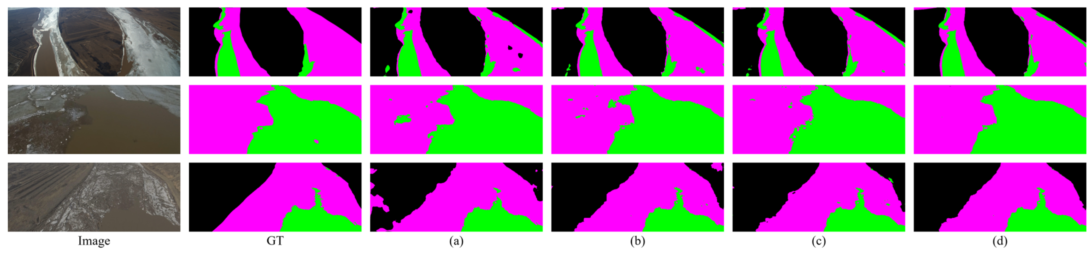
Furthermore, from the visualization results in Figure 11, the differences between different skip connection strategies can be observed more intuitively. Traditional concatenation fusion and SDI tend to produce boundary blurring and local misclassifications near the riverbanks. While SAFM improves some edge quality, prediction fractures still exist for narrow shore ice. In comparison, GDCM can more accurately restore the irregular ice margins near the riverbanks, making the ice–water boundaries smoother and more continuous, while significantly reducing false positives and false negatives in the riverbank areas, verifying the critical role of joint geometric-directional modeling for river ice segmentation.

3.5.4. Effectiveness Analysis of HWD

To analyze the impact of different downsampling strategies on river ice segmentation performance, this study compares Convolution, Average Pooling, Max Pooling, and HWD, with the experimental results presented in

Table 7. Comparison of different downsampling strategies on the NWPU_YRCC_EX dataset.

Models	Setting	IoU (%)			mIoU (%)
		Ice	Water	Other
(a)	Convolution	94.08	89.78	92.95	92.27
(b)	Average Pooling	94.25	89.87	93.68	92.60
(c)	Max Pooling	94.47	90.06	94.53	93.02
(d)	HWD	94.65	90.27	95.31	93.41

.

As shown in Table 7, convolution-based downsampling, average pooling, and max pooling achieve mIoU values of 92.27%, 92.60%, and 93.02%, respectively. Although these traditional downsampling methods can effectively reduce computational complexity, they inevitably cause the loss of high-frequency detail information, performing inadequately on small-scale, complex-boundary broken ice targets. In contrast, after employing HWD in this study, the overall mIoU of the model increases to 93.41%, an improvement of 1.14 percentage points over traditional convolution. Simultaneously, the Ice category IoU reaches 94.65% and the Water category reaches 90.27%, both achieving optimal results. This indicates that the Haar wavelet can simultaneously retain low-frequency structural information and high-frequency edge details during the downsampling process, alleviating the information aliasing problem caused by traditional pooling.

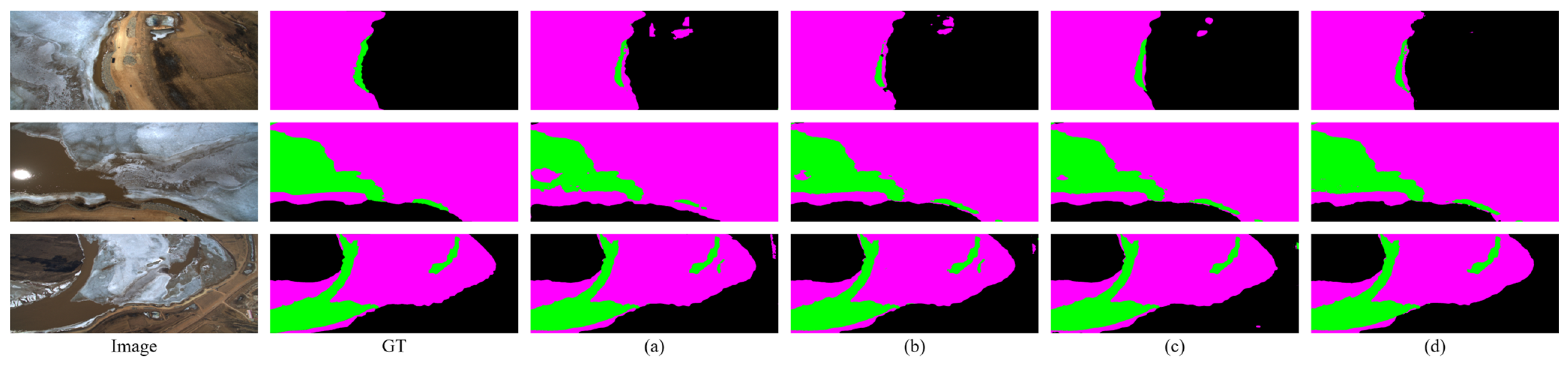
As shown in Figure 12, when traditional convolution is used, dense broken ice areas are prone to target omission and edge blurring. Although average pooling and max pooling can retain some regional information, problems of fragmented ice block adhesion and incomplete boundaries remain. However, after adopting HWD, a large number of minute broken ice pieces are completely preserved, the intervals between ice blocks are clearer, and the ice–water boundaries are more accurate, proving that frequency-domain downsampling can effectively enhance the model’s retention capability for small-scale targets and complex texture regions.

4. Conclusions

In this study, we proposed an efficient and accurate network for river ice semantic segmentation-IceRWKV. To address the inherent trade-off between long-range dependency modeling and computational efficiency, IceRWKV introduces a linear sequence-modeling architecture and develops a novel CC-RWKV block. By integrating multidirectional spatial scanning with context clustering, the proposed module efficiently captures complementary global and local features with linear computational complexity. In addition, a GDCM is designed to accommodate the highly irregular morphology of river ice and suppress background interference. This module enables accurate spatial reconstruction through adaptive geometric correction and polarized feature refinement. HWD is further introduced to preserve the high-frequency boundary information of small ice fragments. Comprehensive experiments on three datasets demonstrate that IceRWKV achieves a favorable balance between segmentation accuracy and inference efficiency, establishing a new state of the art for automated river ice mapping.

Despite its strong segmentation performance, the proposed method remains constrained by the limited sample sizes and scene diversity of existing river ice remote sensing datasets. The robustness of its feature representations under pronounced seasonal variations and extreme illumination conditions therefore requires further investigation. Future work will focus on constructing large-scale river ice datasets with broader spatial and temporal coverage to further improve the generalization capability of the model.

References

1. Ansari, S.; Rennie, C.D.; Clark, S.P.; Seidou, O. IceMaskNet: River Ice Detection and Characterization Using Deep Learning Algorithms Applied to Aerial Photography. Cold Reg. Sci. Technol. 2021, 189, 103324. [Google Scholar] [CrossRef]
2. Kempema, E.W.; Ettema, R. Anchor Ice Rafting: Observations from the Laramie River. River Res. Appl. 2011, 27, 1051–1061. [Google Scholar] [CrossRef]
3. Tang, G.; Zhu, Y.; Wu, G.; Li, J.; Li, Z.-L.; Sun, J. Modelling and Analysis of Hydrodynamics and Water Quality for Rivers in the Northern Cold Region of China. Int. J. Environ. Res. Public Health 2016, 13, 408. [Google Scholar] [CrossRef] [PubMed]
4. Zhang, F.; Elshamy, M.; Lindenschmidt, K.-E. Climate Change Impacts on Ice Jam Behavior in an Inland Delta: A New Ice Jam Projection Framework. Clim. Change 2022, 171, 13. [Google Scholar] [CrossRef]
5. Beltaos, S. Resistance of River Ice Covers to Mobilization and Implications for Breakup Progression in Peace River, Canada. Hydrol. Processes 2023, 37, e14850. [Google Scholar] [CrossRef]
6. Burrell, B.C.; Beltaos, S.; Turcotte, B. Effects of Climate Change on River-Ice Processes and Ice Jams. Int. J. River Basin Manag. 2023, 21, 421–441. [Google Scholar]
7. Yang, X.; Pavelsky, T.M.; Allen, G.H. The Past and Future of Global River Ice. Nature 2020, 577, 69–73. [Google Scholar] [CrossRef] [PubMed]
8. Engram, M.; Arp, C.D.; Jones, B.M.; Ajadi, O.A.; Meyer, F.J. Analyzing Floating and Bedfast Lake Ice Regimes across Arctic Alaska Using 25 Years of Space-Borne SAR Imagery. Remote Sens. Environ. 2018, 209, 660–676. [Google Scholar] [CrossRef]
9. Beaton, A.; Whaley, R.; Corston, K.; Kenny, F. Identifying Historic River Ice Breakup Timing Using MODIS and Google Earth Engine in Support of Operational Flood Monitoring in Northern Ontario. Remote Sens. Environ. 2019, 224, 352–364. [Google Scholar] [CrossRef]
10. Ijitona, T.B.; Ren, J.; Hwang, P.B. SAR Sea Ice Image Segmentation Using Watershed with Intensity-Based Region Merging. In Proceedings of the 2014 IEEE International Conference on Computer and Information Technology; IEEE: Xi’an, China, 2014; pp. 168–172. [Google Scholar]
11. Liu, J.; Scott, K.A.; Gawish, A.; Fieguth, P. Automatic Detection of the Ice Edge in SAR Imagery Using Curvelet Transform and Active Contour. Remote Sens. 2016, 8, 480. [Google Scholar] [CrossRef]
12. Zhang, Q.; Skjetne, R.; Metrikin, I.; Løset, S. Image Processing for Ice Floe Analyses in Broken-Ice Model Testing. Cold Reg. Sci. Technol. 2015, 111, 27–38. [Google Scholar] [CrossRef]
13. Chu, T.; Lindenschmidt, K.-E. Integration of Space-Borne and Air-Borne Data in Monitoring River Ice Processes in the Slave River, Canada. Remote Sens. Environ. 2016, 181, 65–81. [Google Scholar] [CrossRef]
14. Park, J.-W.; Korosov, A.A.; Babiker, M.; Won, J.-S.; Hansen, M.W.; Kim, H.-C. Classification of Sea Ice Types in Sentinel-1 Synthetic Aperture Radar Images. Cryosphere 2020, 14, 2629–2645. [Google Scholar] [CrossRef]
15. Ren, J.; Hwang, B.; Murray, P.; Sakhalkar, S.; McCormack, S. Effective SAR Sea Ice Image Segmentation and Touch Floe Separation Using a Combined Multi-Stage Approach. In Proceedings of the 2015 IEEE International Geoscience and Remote Sensing Symposium (IGARSS); IEEE: Milan, Italy, 2015; pp. 1040–1043. [Google Scholar]
16. Kalke, H.; Loewen, M.R. Support Vector Machine Learning Applied to Digital Images of River Ice Conditions. Cold Reg. Sci. Technol. 2018, 155, 225–236. [Google Scholar] [CrossRef]
17. Liu, H.; Guo, H.; Zhang, L. SVM-Based Sea Ice Classification Using Textural Features and Concentration from RADARSAT-2 Dual-Pol ScanSAR Data. IEEE J. Sel. Top. Appl. Earth Obs. Remote Sens. 2014, 8, 1601–1613. [Google Scholar]
18. Shu, S.; Zhou, X.; Shen, X.; Liu, Z.; Tang, Q.; Li, H.; Ke, C.; Li, J. Discrimination of Different Sea Ice Types from CryoSat-2 Satellite Data Using an Object-Based Random Forest (ORF). Mar. Geod. 2020, 43, 213–233. [Google Scholar]
19. Wang, J.; Cao, Z.; Fu, S.; Kang, Z.; Wang, J. A Novel Flexible Architecture Based on SAM for Automatic Exraction of Rampart Craters From Martian High Resolution Images. IEEE J. Sel. Top. Appl. Earth Obs. Remote Sens. 2025, 18, 21129–21143. [Google Scholar] [CrossRef]
20. Fu, S.; Gu, Z.; Wang, Y.; Zhang, L.; Gu, H.; Wu, J.; Liao, G. D2Mamba: A Mamba-Based Method for Floodway Obstructions Segmentation from Multispectral Satellite Imagery. J. Hydrol. 2026, 669, 135069. [Google Scholar] [CrossRef]
21. Qiao, X.; Roy, S.K.; Huang, W. 3-D Sharpened Cosine Similarity Operation for Hyperspectral Image Classification. IEEE J. Sel. Top. Appl. Earth Obs. Remote Sens. 2023, 17, 1114–1125. [Google Scholar]
22. Qiao, X.; Roy, S.K.; Huang, W. Multiscale Neighborhood Attention Transformer with Optimized Spatial Pattern for Hyperspectral Image Classification. IEEE Trans. Geosci. Remote Sens. 2023, 61, 5523815. [Google Scholar] [CrossRef]
23. Qiao, X.; Huang, W. A Dual Frequency Transformer Network for Hyperspectral Image Classification. IEEE J. Sel. Top. Appl. Earth Obs. Remote Sens. 2023, 16, 10344–10358. [Google Scholar] [CrossRef]
24. Zhou, D.; Wu, K.; Hu, J.; Sun, Q. Enhancing DeepLabv3+ with Multi-Scale Sparse-Aware Dilated Convolution and Boundary-Interactive ASPP for River Ice Segmentation. IEEE Geosci. Remote Sens. Lett. 2026, 23, 15. [Google Scholar] [CrossRef]
25. Wu, K.; Zhou, D.; Du, J.; Wu, Y.; Zhang, L. IceSegNet: A Stage-Aware Dynamic Kernel Network for River Ice Segmentation in Remote Sensing Imagery. Appl. Soft Comput. 2025, 186, 114120. [Google Scholar] [CrossRef]
26. Zhang, X.; Zhao, Z.; Ran, L.; Xing, Y.; Wang, W.; Lan, Z.; Yin, H.; He, H.; Liu, Q.; Zhang, B. FastICENet: A Real-Time and Accurate Semantic Segmentation Model for Aerial Remote Sensing River Ice Image. Signal Process. 2023, 212, 109150. [Google Scholar] [CrossRef]
27. Wang, Z.; Li, Y.; Wang, Y.; Gu, H.; Zhang, L. Patch-Based Transformer Network Construction with Adaptive Feature-Interaction for Hyperspectral Image Classification. IEEE Trans. Geosci. Remote Sens. 2024, 62, 5533013. [Google Scholar] [CrossRef]
28. Shamshad, F.; Khan, S.; Zamir, S.W.; Khan, M.H.; Hayat, M.; Khan, F.S.; Fu, H. Transformers in Medical Imaging: A Survey. Med. Image Anal. 2023, 88, 102802. [Google Scholar] [CrossRef] [PubMed]
29. Hu, Y.; Wang, Z.; Huang, Z.; Liu, Y. PolyBuilding: Polygon Transformer for Building Extraction. ISPRS J. Photogramm. Remote Sens. 2023, 199, 15–27. [Google Scholar] [CrossRef]
30. Pinheiro, M.M.F.; de Oliveira, L.Y.D.; Venancio, T.E.B.; Nogueira, K.; Júnior, J.M.; Gonçalves, W.N.; Pereira, D.R.; Osco, L.P.; Ramos, A.P.M. Deep Learning on Segmenting Large and Narrow Rivers with Aerial RGB imagery: A Comparison of Convolutional and Vision-Transformer Networks. Remote Sens. Appl. Soc. Environ. 2026, 42, 101970. [Google Scholar] [CrossRef]
31. Wei, C.; Li, H.; Chen, L.; Zhou, H.; Taukebayev, O.; Wu, W.; Temirbayev, A.; Han, L.; Ran, L.; Yin, H. River Ice Fine-Grained Segmentation: A GF-2 Satellite Image Dataset and Deep Learning Benchmark. IEEE Trans. Geosci. Remote Sens. 2025, 63, 5407115. [Google Scholar] [CrossRef]
32. Zhu, Z.; Qi, Y.; Li, H.; Chen, L.; Wei, C.; Zhang, X. MixFormer: A Unified Vision Transformer for River Ice Semantic Segmentation of Multisource Remote Sensing Imagery. In Proceedings of the 2025 5th International Conference on Computer Systems (ICCS); IEEE: Xi’an, China, 2025; pp. 70–76. [Google Scholar]
33. Wang, Q.; Zhong, H.; Xu, C.; Shen, T. RS 3-RWKV: Leveraging RWKV for Efficient Remote Sensing Semantic Segmentation. IEEE J. Sel. Top. Appl. Earth Obs. Remote Sens. 2025, 18, 27372–27383. [Google Scholar] [CrossRef]
34. He, Q.; Zhang, J.; Peng, J.; He, H.; Li, X.; Wang, Y.; Wang, C. Pointrwkv: Efficient Rwkv-like Model for Hierarchical Point Cloud Learning. In Proceedings of the AAAI Conference on Artificial Intelligence; AAAI Press: Washington, DC, USA, 2025; Volume 39, pp. 3410–3418. [Google Scholar]
35. Hou, H.; Huang, Z.; Tan, K.; Lu, R.; Yu, F.R. Rwkv-x: A Linear Complexity Hybrid Language Model. arXiv 2025, arXiv:2504.21463. [Google Scholar]
36. Liu, H.; Man, H.; Wang, X.; Li, W.; Zhao, D. MRT: Learning Compact Representations with Mixed RWKV-Transformer for Extreme Image Compression. In Proceedings of the Proceedings of the AAAI Conference on Artificial Intelligence; AAAI Press: Washington, DC, USA, 2026; Volume 40, pp. 7141–7149. [Google Scholar]
37. Zhang, X.; Zhou, Y.; Jin, J.; Wang, Y.; Fan, M.; Wang, N.; Zhang, Y. ICENETv2: A Fine-Grained River Ice Semantic Segmentation Network Based on UAV Images. Remote Sens. 2021, 13, 633. [Google Scholar] [CrossRef]
38. Singh, A.; Kalke, H.; Loewen, M.; Ray, N. River Ice Segmentation with Deep Learning. IEEE Trans. Geosci. Remote Sens. 2020, 58, 7570–7579. [Google Scholar] [CrossRef]
39. Tang, F.; Ding, J.; Quan, Q.; Wang, L.; Ning, C.; Zhou, S.K. Cmunext: An Efficient Medical Image Segmentation Network Based on Large Kernel and Skip Fusion. In Proceedings of the 2024 IEEE International Symposium on Biomedical Imaging (ISBI); IEEE: Athens, Greece, 2024; pp. 1–5. [Google Scholar]
40. Xu, G.; Liao, W.; Zhang, X.; Li, C.; He, X.; Wu, X. Haar Wavelet Downsampling: A Simple but Effective Downsampling Module for Semantic Segmentation. Pattern Recognit. 2023, 143, 109819. [Google Scholar] [CrossRef]
41. Xu, J.; Xiong, Z.; Bhattacharyya, S.P. PIDNet: A Real-Time Semantic Segmentation Network Inspired from PID Controller. arXiv 2022, arXiv:2206.02066. [Google Scholar]
42. Yu, C.; Wang, J.; Peng, C.; Gao, C.; Yu, G.; Sang, N. Bisenet: Bilateral Segmentation Network for Real-Time Semantic Segmentation. In Proceedings of the Proceedings of the European Conference on Computer Vision (ECCV); Springer: Berlin/Heidelberg, Germany, 2018; pp. 325–341. [Google Scholar]
43. Poudel, R.P.; Bonde, U.; Liwicki, S.; Zach, C. Contextnet: Exploring Context and Detail for Semantic Segmentation in Real-Time. arXiv 2018, arXiv:1805.04554. [Google Scholar]
44. Wang, L.; Li, R.; Zhang, C.; Fang, S.; Duan, C.; Meng, X.; Atkinson, P.M. UNetFormer: A UNet-like Transformer for Efficient Semantic Segmentation of Remote Sensing Urban Scene Imagery. ISPRS J. Photogramm. Remote Sens. 2022, 190, 196–214. [Google Scholar] [CrossRef]
45. Wang, L.; Fang, S.; Meng, X.; Li, R. Building Extraction with Vision Transformer. IEEE Trans. Geosci. Remote Sens. 2022, 60, 5625711. [Google Scholar] [CrossRef]
46. Ding, M.; Xiao, B.; Codella, N.; Luo, P.; Wang, J.; Yuan, L. Davit: Dual Attention Vision Transformers. In Proceedings of the European Conference on Computer Vision; Springer: Berlin/Heidelberg, Germany, 2022; pp. 74–92. [Google Scholar]
47. Zhang, X.; Jin, J.; Lan, Z.; Li, C.; Fan, M.; Wang, Y.; Yu, X.; Zhang, Y. ICENET: A Semantic Segmentation Deep Network for River Ice by Fusing Positional and Channel-Wise Attentive Features. Remote Sens. 2020, 12, 221. [Google Scholar] [CrossRef]
48. Duan, Y.; Wang, W.; Chen, Z.; Zhu, X.; Lu, L.; Lu, T.; Qiao, Y.; Li, H.; Dai, J.; Wang, W. Vision-Rwkv: Efficient and Scalable Visual Perception with Rwkv-Like Architectures. In Proceedings of the International Conference on Learning Representations, Singapore, 24–28 April 2025; Volume 2025, pp. 83166–83182. [Google Scholar]
49. Ye, H.; Tang, F.; Zhao, P.; Huang, Z.; Zhao, D.; Bian, M.; Zhou, S.K. U-Rwkv: Lightweight Medical Image Segmentation with Direction-Adaptive Rwkv. In Proceedings of the International Conference on Medical Image Computing and Computer-Assisted Intervention; Springer: Berlin/Heidelberg, Germany, 2025; pp. 613–623. [Google Scholar]
50. Ronneberger, O.; Fischer, P.; Brox, T. U-Net: Convolutional Networks for Biomedical Image Segmentation. In Proceedings of the International Conference on Medical Image Computing and Computer-Assisted Intervention; Springer: Berlin/Heidelberg, Germany, 2015; pp. 234–241. [Google Scholar]
51. Peng, Y.; Chen, D.Z.; Sonka, M. U-Net v2: Rethinking the Skip Connections of u-Net for Medical Image Segmentation. In Proceedings of the 2025 IEEE 22nd International Symposium on Biomedical Imaging (ISBI); IEEE: Houston, TX, USA, 2025; pp. 1–5. [Google Scholar]
52. Yao, M.; Hu, G.; Zhang, Y. CG-Fclnet: Category-Guided Feature Collaborative Learning Network for Semantic Segmentation of Remote Sensing Images. Comput. Mater. Contin. 2025, 83, 2751–2771. [Google Scholar] [CrossRef]
Figure 1. Overall structure of the proposed RWKV.
Remotesensing 18 02683 g001
Figure 2. Structure of the CC-RWKV block.
Remotesensing 18 02683 g002
Figure 3. Structure of the GDCM.
Remotesensing 18 02683 g003
Figure 4. Architectural schematic of the HWD.
Remotesensing 18 02683 g004
Figure 5. Representative samples from the three datasets. (a) Images and corresponding annotations from NWPU_YRCC_EX, where black, green, and purple denote shore, water, and ice, respectively; (b) samples from NWPU_YRCC2, where black, green, blue, and purple denote shore, water, shore ice, and drift ice, respectively; and (c) samples from the Alberta River Ice Segmentation Dataset, where white, gray, and black denote drift ice, anchor ice, and water, respectively.
Remotesensing 18 02683 g005
Figure 6. Visual comparison of images on the NWPU_YRCC_EX Dataset using the 10 selected methods. The protruding parts are indicated by solid-line boxes.
Remotesensing 18 02683 g006
Figure 7. Visual comparison of images on the NWPU_YRCC2 Dataset using the 10 selected methods. The protruding parts are indicated by solid-line boxes.
Remotesensing 18 02683 g007
Figure 8. Visual comparison of images on the Alberta River Ice Segmentation Dataset using the 10 selected methods.
Remotesensing 18 02683 g008
Figure 9. Visual comparison of different configurations in the overall ablation study. (a) Baseline; (b) Baseline + CC-RWKV; (c) Baseline + GDCM; (d) Baseline + HWD; (e) Baseline + CC-RWKV + GDCM; (f) Baseline + CC-RWKV + HWD; (g) Baseline + GDCM + HWD; (h) Baseline + CC-RWKV + GDCM + HWD.
Remotesensing 18 02683 g009
Figure 10. Visual comparison of different RWKV modeling strategies. (a) CMUNeXt Block; (b) Unidirectional RWKV; (c) Quad-WKV; (d) CC-RWKV (ours).
Remotesensing 18 02683 g010
Figure 11. Visual comparison of different skip connection strategies. (a) Concatenation; (b) SDI; (c) SAFM; (d) GDCM.
Remotesensing 18 02683 g011
Figure 12. Visual comparison of different downsampling strategies. (a) Convolution; (b) Average Pooling; (c) Max Pooling; (d) HWD.
Remotesensing 18 02683 g012