High-Resolution Aboveground Biomass Estimates of Tropical Peatland Forest Based on Planet NICFI Imagery and Airborne LiDAR

Highlights

What are the main findings?

• DL-PowerReg approach achieved higher accuracy in aboveground biomass (AGB) estimation (MAE = 52.24 t/ha) than the StepwiseReg-DL approach (MAE = 62.08 t/ha).
• High-resolution Planet imagery effectively complemented spatially limited LiDAR observations, enabling wall-to-wall forest AGB mapping in the study area.

What are the implications of the main findings?

• In addition to improving AGB estimation accuracy, DL-PowerReg generates a canopy height model (CHM) as an intermediate product, providing valuable information for a more comprehensive assessment of forest structure and condition.
• The methodological frameworks offer approaches for high-resolution forest biomass estimation in regions where LiDAR coverage is limited but satellite imagery is readily available.

Abstract

Peat swamp forests play a critical role in maintaining the ecological integrity of tropical peatlands. The conservation and restoration efforts on these ecosystems have gained considerable attention considering their vulnerability. Accurate spatial mapping of aboveground biomass (AGB) is important to support such measures, and it can be accurately implemented using airborne LiDAR. However, the high operational cost of LiDAR surveys typically restricts their spatial coverage. This study estimated AGB of peat swamp forests by combining two remote sensing datasets, i.e., Planet NICFI imagery (2023–2024) and partially covered airborne LiDAR (10.56% of the total area), in the Katingan–Mentaya peat swamp forest, Central Kalimantan, Indonesia. Two workflows were proposed and compared. The first, DL-PowerReg, estimated canopy height model (CHM) using a U-Net deep learning model trained on Planet imagery, followed by AGB mapping through power regression. The second, StepwiseReg-DL, derived LiDAR-based AGB through stepwise regression of LiDAR metrics, then upscaled it to the full study area using U-Net with Planet imagery as input. DL-PowerReg (MAE = 52.24 t/ha) outperformed StepwiseReg-DL (MAE = 62.08 t/ha) and additionally produced an intermediate CHM map, providing complementary information on forest structure. The two approaches estimated total AGB storage in the study area at 47.75 Mt (mean = 239.91 t/ha) and 40.07 Mt (mean = 201.30 t/ha), respectively. This study demonstrates a methodological framework for leveraging spatially incomplete LiDAR data in high-resolution wall-to-wall forest biomass mapping.

1. Introduction

Tropical forests are one of the most important terrestrial ecosystems in the global carbon cycle [1]. As the largest forest biomes, covering about 12% of the Earth’s land surface, they store the highest aboveground living biomass of any biome, accounting for 371.5 Gt C [2]. Lying elongated around the equatorial line, Indonesian tropical forests store about 15 Gt C [3]. In addition, about 11% (20.4 million ha) of the country’s land area is categorized as peatlands, one of the largest in the tropics, storing 55 ± 10 Gt of soil carbon [4,5]. The pressure from anthropogenic activities has led to a massive peatland degradation alongside a land use conversion into plantations and agriculture [6]. The unfavorable land conversions are incompatible with the natural condition of waterlogged peatlands; thus, peat soils are decomposed and oxidized, and they become susceptible to recurrent fires [7,8]. Therefore, the peat swamp forest coverage in tropical peatlands is essential not only to store its own aboveground standing biomass but also to preserve the peat soils from degradation in their natural conditions in order to minimize carbon emissions.

In response to the Paris Agreement, Indonesia has launched the FOLU Net Sink 2030 initiative, aiming for the Forestry and Other Land Use (FOLU) sector to become a net carbon sink by 2030 [9]. This strategy includes measures like reducing deforestation, restoring degraded land and peatlands, and improving sustainable forest management and complements climate action tools such as REDD+ (Reducing Emissions from Deforestation and Forest Degradation). One worthy action is by way of ecosystem restoration concession regulations, which grant private sectors the ability to carry out restoration through multiuse forest management instead of timber harvesting [10]. Being leased a working area in a degraded peatland area of Katingan–Mentaya Peat Hydrological Unit, PT Rimba Makmur Utama (PT RMU) implements restoration programs, including reforestation, rewetting, and supporting sustainable livelihoods in the surrounding area [11]. To support achieving the targets, an accurate spatial assessment of the forest state is necessary, particularly on aboveground biomass and forest structure.

By leveraging spatial and temporal dimensions, remote sensing technology coupled with the advancement of machine learning answers the needs of efficient and actual information about the state of forests and their carbon balance [12,13]. Among remote sensing modes, airborne LiDAR (light detection and ranging) offers highly precise three-dimensional point cloud data to observe vegetation structure [14], and it is often integrated with forest inventory to estimate high-accuracy forest biomass at the tree as well as the stand level [15,16]. Despite its eminence, there exists an expensive operational cost of the LiDAR survey, thus restraining the data acquisition from being implemented in a larger spatial extent. Another source of LiDAR data to measure forest structure is from a space-based mission such as GEDI and ICESat/ICESat-2. Nevertheless, these datasets are sparse and have a limited number of valid observations in Indonesian tropical forests.

To describe beyond the coverage area, LiDAR data is often integrated with satellite-based images in order to extrapolate the information obtained by the LiDAR sensor. For instance, using the reference data of GEDI-based canopy height, previous studies have demonstrated regional- and global-scale forest height mapping based on multispectral medium-resolution imageries such as Landsat and Sentinel-2 images [17,18,19] as well as combinations of radar and multispectral images [20,21,22]. For more detailed canopy height mapping, some studies employed the upscaling methods using airborne LiDAR (or combined with spaceborne LiDAR) and higher resolution images, e.g., Planet [23], Maxar [24], and aerial images [25,26]. Among high-resolution datasets, Planet NICFI Basemaps offer a promising data source for LiDAR upscaling because they provide freely accessible monthly mosaics at 4.77 m spatial resolution across tropical regions, enabling detailed wall-to-wall mapping beyond the LiDAR coverage [23,27,28].

Considering the relationship between tree height and its biomass, the modeled canopy height can subsequently predict aboveground biomass and carbon stock with a regression model [29,30]. Another approach is multi-level AGB mapping: estimating AGB using LiDAR data, then using it as a reference for prediction using satellite imagery. The initial step commonly entails point cloud metrics that describe vertical and horizontal vegetation structure for LiDAR-based AGB prediction [31,32]. Similar to the extrapolation of LiDAR-based information, the AGB estimate in the second step of multi-level mapping can also be achieved by means of machine learning [32]. Although deep learning-based AGB has been widely used, the implementation in this multi-stage method is still scarce. Nevertheless, deep learning is more capable of capturing spatial context compared to regressions and traditional machine learning algorithms when working with images with uncertain radiometric accuracy like the Planet NICFI mosaic [23]. While previous studies have presented two different frameworks—the CHM approach and the multi-level method—in assessing AGB from incomplete LiDAR data coverage, the comparison has not been investigated, particularly for high-resolution mapping. Furthermore, high-resolution imagery is advantageous for AGB mapping because it captures fine-scale canopy heterogeneity, reduces mixed-pixel effects, and provides spatial information that can improve biomass estimation accuracy [33].

Having been proven in its capability in remote sensing-based modeling, the deep learning method of Convolutional Neural Networks (CNNs) is capable of learning spatial patterns for mapping vegetation properties through the extraction of spatial and texture features [34]. U-Net, one of CNN architectures, is specialized in image analysis by employing encoder–decoder and skip connections to capture context and give strong localization while preserving the resolution, making it well suited for dense pixel-level regression tasks such as CHM and forest biomass estimation [35]. In addition, U-Net can be trained effectively with relatively limited datasets and has demonstrated robust performance in remote sensing applications [36,37]. This U-Net framework has shown accurate predictions of canopy height [21,26] and biomass [38].

Existing approaches for estimating AGB from incomplete LiDAR coverage have not been comparatively evaluated for high-resolution mapping, motivating this study’s assessment of CHM- and multi-level-based frameworks. This present study aims to scrutinize the different approaches in estimating AGB using three available datasets: (1) partially covered airborne LiDAR, (2) Planet NICFI images, and (3) field inventory data in the Katingan–Mentaya peat swamp forest. The first approach consists of canopy height modeling in the entire study area using the U-Net deep learning model followed by AGB mapping through power regression. The second approach begins with LiDAR-based biomass mapping in the partial area and then applies a deep learning model to the whole study area.

2. Study Area

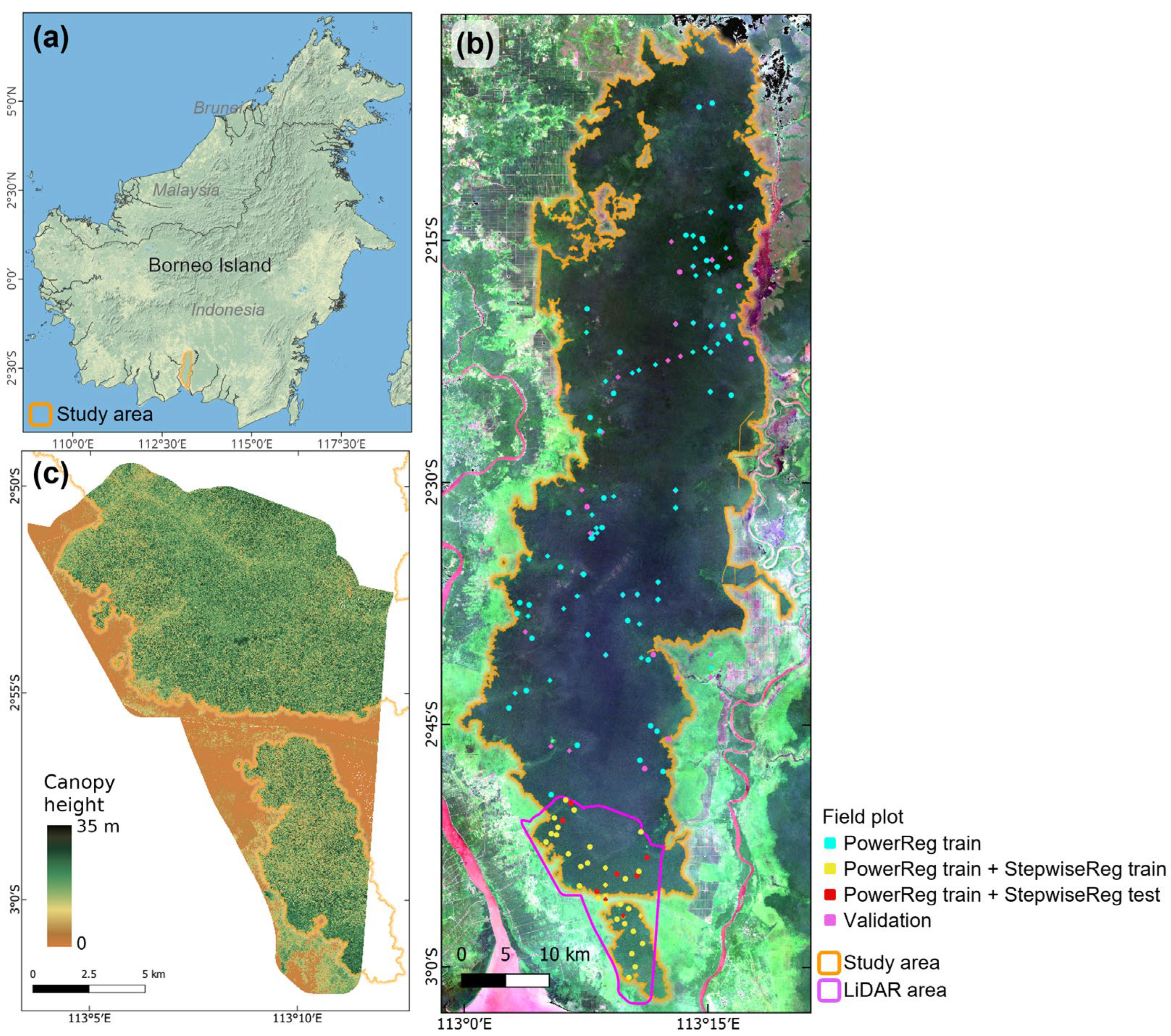
The study area is located in the peat swamp forest of the Katingan River and Mentaya River Peat Hydrological Unit, Central Kalimantan, Indonesia, named after two rivers sandwiching the peatland area (2°29′20″S, 113°10′31″E) (Figure 1). The Indonesian government has granted this area to be managed by PT Rimba Makmur Utama (PT RMU) under the ecosystem restoration concession scheme. This project aims to restore the peatland ecosystem in 60 years until 2073 [11]. Prior to the restoration measures, most of the forested areas had been exposed to logging operations for decades, with some areas further degraded by fire events. The cleared land was then converted into cultivation and plantation areas, such as rice fields, rubber plantations, and oil palm plantations. Although some areas remained forested, they had already been disturbed, as large, healthy trees had been harvested and removed, resulting in a significant loss of biomass. Nevertheless, undisturbed forest patches still persist, particularly in the middle of the peatland area.

The peat layers are estimated to reach up to 12 m thickness in the middle part, whereas two-thirds of the area has a depth between 4 and 8 m [11]. A survey by Harrison et al. [39] reported the richness of vegetation composition in this area with a total of 204 confirmed floral species, showing the relatively high diversity and comparability to the neighboring Sebangau National Park on the east side. The extent of the PT RMU concession area is 157,875 ha, yet it does not fully cover the hydrological unit area. Therefore, instead of limiting the study area based on the restoration area, we extended our study area to cover all forest areas within the peat hydrological unit of Katingan–Mentaya with a total area of 198,919 ha.

3. Materials and Methods

3.1. LiDAR Dataset

LiDAR data were collected from an airborne survey in August 2022 covering 210 km² in the southern part, representing 10.56% of the total study area. The data acquisition used a Leica DragonEye (Leica Geosystems AG, Heerbrugg, Switzerland) working at near-infrared light (1064 nm) with an ability to capture up to 1 MHz of data (1 million points per second). After post-processing and classification, the LiDAR density became 7.3 points/m² with a vertical accuracy of 0.15 m. We first generated a Digital Terrain Model (DTM) and Digital Surface Model (DSM) from ground points and non-ground points, respectively, at 1 m resolution. The Canopy height model (CHM) was derived from the subtraction between the DSM and DTM.

3.2. Planet Imagery

Norway’s International Climate and Forest Initiative (NICFI) enabled the public access of the visual basemap product of Planet imagery in the tropics between 30°N and 30°S [40]. The monthly Planet mosaic is available from September 2020 onwards at a spatial resolution of 4.77 m and contains 4 bands, i.e., blue, green, red, and near-infrared. We obtained Planet imagery using the Google Earth Engine geospatial cloud computing platform. We selected 5 monthly mosaics consisting of April 2023, October 2023, July 2024, September 2024, and December 2024, considering the least presence of clouds, haze, and cloud shadows. However, clouds are still inevitable in the selected images; therefore, first we masked atmospheric disturbances by applying a reflectance value threshold of 400 (scale = 0.0001) in the blue band and then performed a median temporal mosaic. We clipped the digital values of RGB bands in the range of 0–50%, while leaving the near-infrared band values unclipped. This method was intended to enhance the spectral values of vegetation in visible bands, which are typically low, adopting the data pre-processing in Dalagnol et al. [27]. All bands were then converted to 8-bit (0–255) and resampled into 5 m resolution to straightforwardly match the LiDAR-based CHM. This conversion optimized computational efficiency while maintaining the number of levels necessary for deep learning [27].

3.3. Forest Inventory

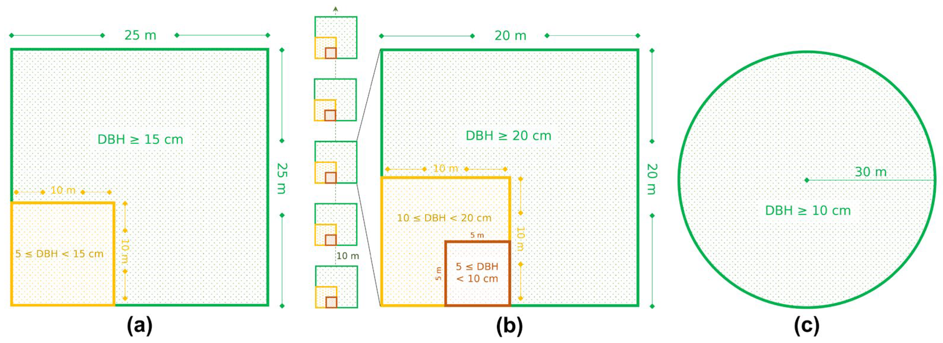
Field surveys were carried out in two different timeframes: the first one in 2022 and the latter in 2023–2024. The first inventory campaign adopted three plot types, yet one plot type was shaped as a long rectangle, which is not appropriate to be used for image analysis. The other two types are basically square, designed with a shape of 25 × 25 m, and a multi-plot design consisting of 5 plots, each having a shape of 20 × 20 m (Figure 2a,b). The second forest inventory used a circular shape with a radius of 30 m (Figure 2c). Several data points were recorded, including diameter at breast height (DBH), tree height, species, and other relevant information. However, tree height was only measured in the second inventory, and even then, only a few trees for each plot. Therefore, here we relied on the DBH to calculate tree AGB using an allometric equation developed by Manuri et al. [41] as follows:

$$AGB=0.136\times {DBH}^{2.513}$$

(1)

where AGB and DBH, respectively, denote tree aboveground biomass in kg and diameter at breast height in cm. This equation was developed for tropical peat swamp forests by taking samples in Sumatra and Kalimantan, Indonesia [41]. To obtain AGB value per plot with a unit in t/ha, we summed the tree AGB of each nested plot, multiplied it by the area factor, and summed all values within the plot.

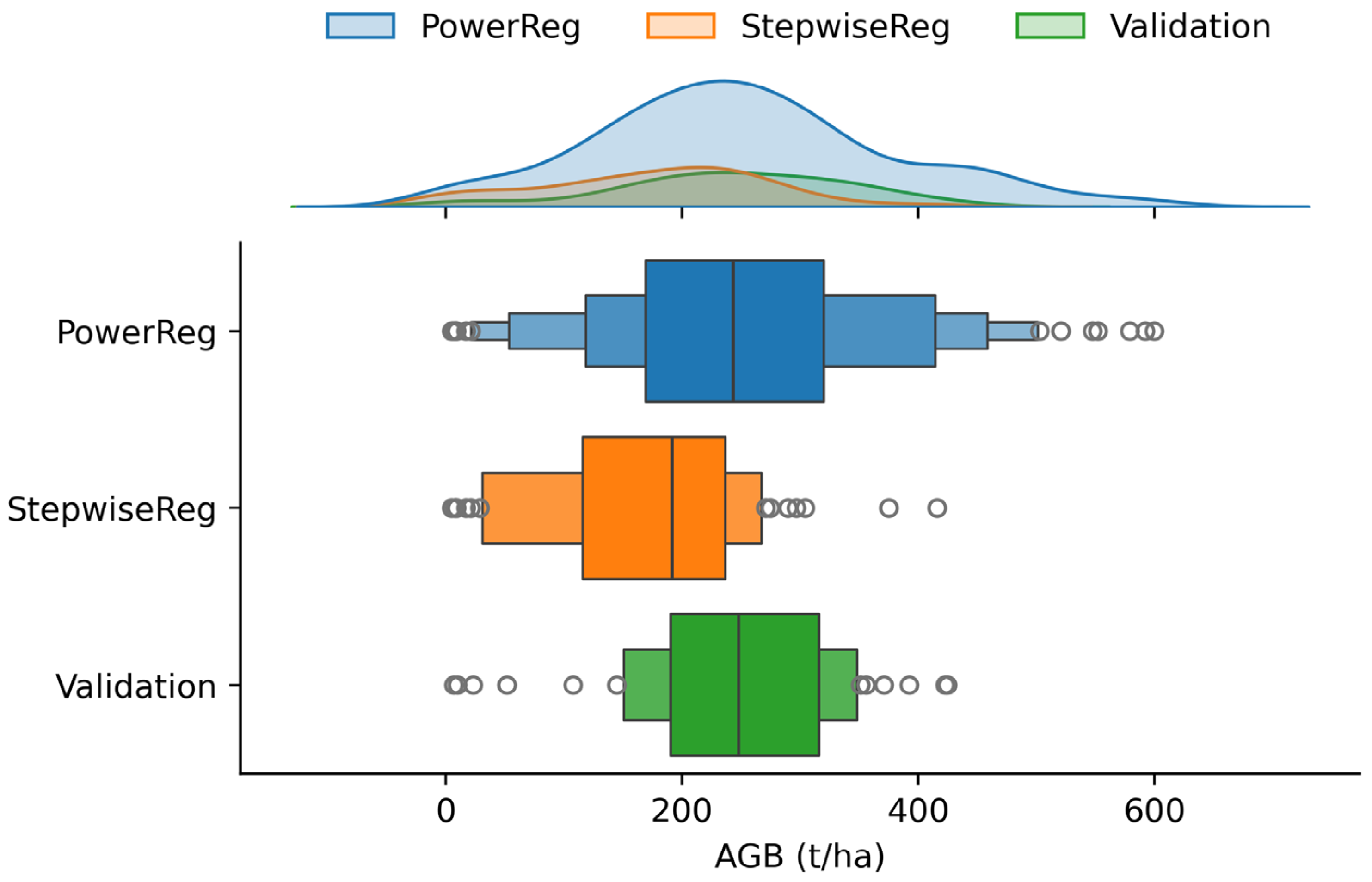
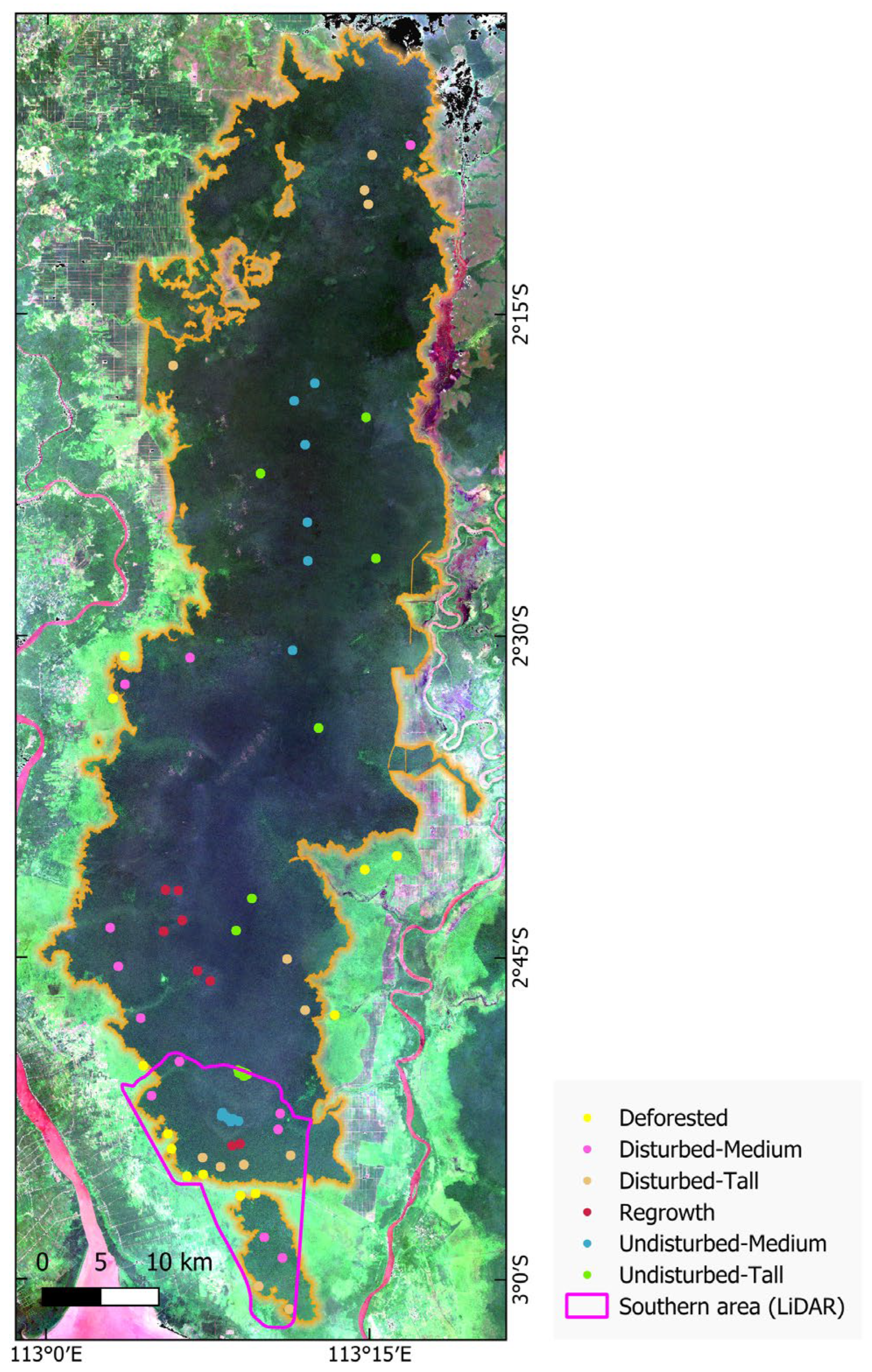
A total of 246 valid field observations were available for analysis. Of these, 49 plots (20%) were reserved as an independent validation dataset to assess the final AGB maps produced by both DL-PowerReg and StepwiseReg-DL models. The remaining 197 plots were used to develop the power regression model for DL-PowerReg. Among these 197 training samples, only 52 were located in the LiDAR-covered area and were therefore used for the stepwise regression analysis in StepwiseReg-DL. These 52 samples were further divided into training and testing subsets, comprising 41 and 11 samples, respectively. The spatial distribution and data distribution of these field plots are presented in Figure 1 and Figure A1.

3.4. Methodology

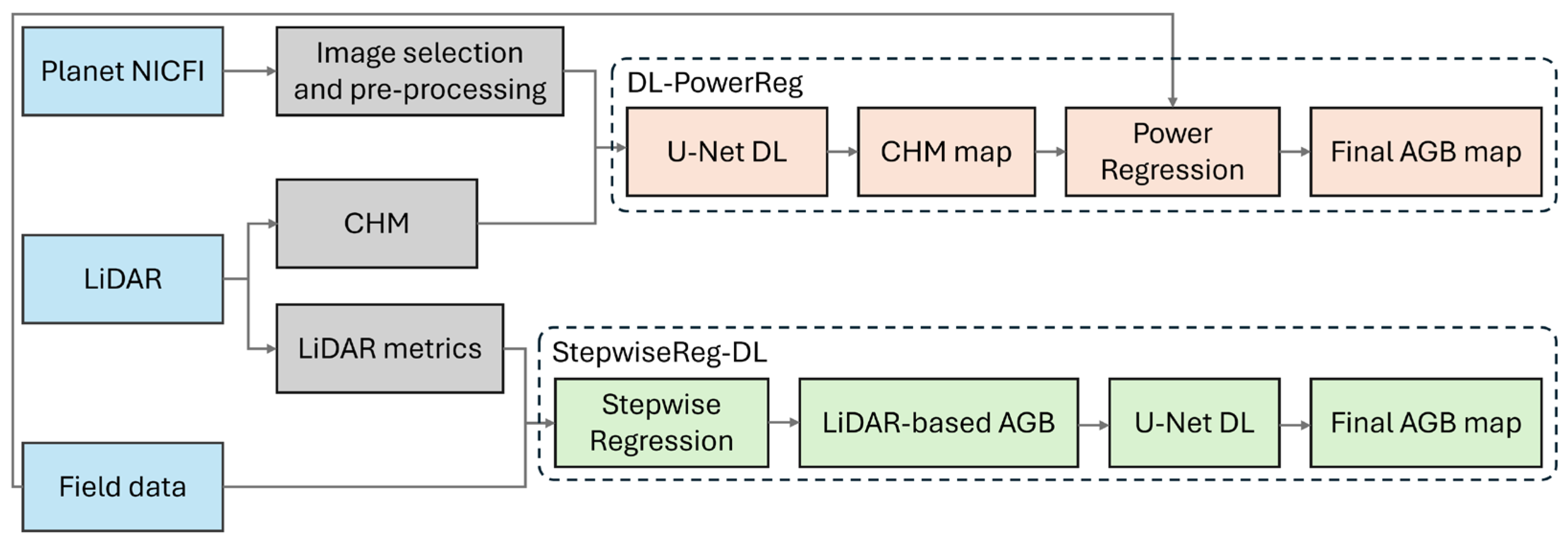
This study investigated two methods in wall-to-wall mapping of AGB based on the workflow using the integration of LiDAR and satellite imagery, namely DL-PowerReg and StepwiseReg-DL (Figure 3).

3.4.1. DL-PowerReg Model

The first approach consists of two steps: (1) estimating the canopy height model (CHM) in the entire study area using deep learning algorithms and (2) employing power regression-based AGB mapping using the estimated CHM and field data.

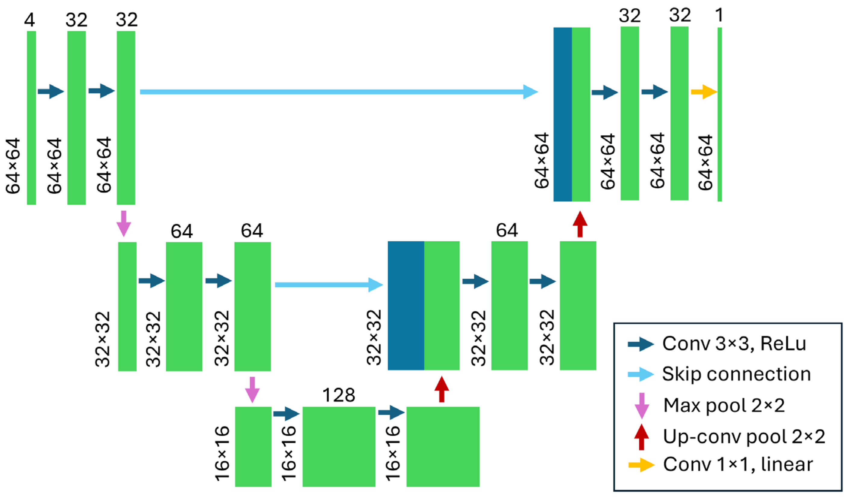
In the first stage, a pixel-wise regression based on U-Net deep learning architecture was adopted to estimate CHM [35]. The model input comprised 4-band Planet imagery, while the label image was a LiDAR-based CHM, all together having a patch size of 64 × 64 pixels. During model development, several deep learning configurations were evaluated, including U-Net and Xception architectures with both their original and shallower network depths. Different input feature combinations were also investigated, i.e., four bands only and their combination with vegetation indices. The shallower U-Net using only the spectral bands achieved the best overall performance. Consequently, a simplified U-Net architecture comprising three encoder blocks and two decoder blocks was adopted (Figure 4 and

Table A1. Summary of U-Net model with a total number of trainable parameters of 466,817.

Layer	Type	Output Size	Parameters
input_layer	InputLayer	64 × 64 × 4	0
conv2d	Conv2D	64 × 64 × 32	1184
conv2d_1	Conv2D	64 × 64 × 32	9248
max_pooling2d	MaxPooling2D	32 × 32 × 32	0
conv2d_2	Conv2D	32 × 32 × 64	18,496
conv2d_3	Conv2D	32 × 32 × 64	36,928
max_pooling2d_1	MaxPooling2D	16 × 16 × 64	0
conv2d_4	Conv2D	16 × 16 × 128	73,856
conv2d_5	Conv2D	16 × 16 × 128	147,584
conv2d_transpose	Conv2DTranspose	32 × 32 × 64	32,832
concatenate	Concatenate	32 × 32 × 128	0
conv2d_6	Conv2D	32 × 32 × 64	73,792
conv2d_7	Conv2D	32 × 32 × 64	36,928
conv2d_transpose_1	Conv2DTranspose	64 × 64 × 32	8224
concatenate_1	Concatenate	64 × 64 × 64	0
conv2d_8	Conv2D	64 × 64 × 32	18,464
conv2d_9	Conv2D	64 × 64 × 32	9248
conv2d_10	Conv2D	64 × 64 × 1	33

). This lighter U-Net architecture decreases the number of parameters to optimize; also, it can reduce overfitting issues [42].

On each level of encoder or contracting path level, the process includes two 3 × 3 two-dimensional convolutions with a rectified linear unit (ReLU) activation function followed by a 2 × 2 max-pooling operation. In the expanding path or decoder, each stage involves a 2 × 2 two-dimensional convolution transpose feature map concatenation with the contracting path, followed by two 3 × 3 two-dimensional convolutions with ReLU activation functions. To deal with a regression task, we used a linear activation in the final layer to produce a single-channel output of continuous data with a dimension of 64 × 64. The model was optimized using the Adam algorithm with a learning rate of 0.0001 and trained for 1000 epochs with a batch size of 32. A custom weighted mean absolute error (MAE) loss function was employed, defined as follows:

$$L={\displaystyle \frac{1}{N}}{\displaystyle \sum _{i=1}^N}\sqrt{yi+1}|yi-\hat{y}i|$$

(2)

where N, yi, and $\hat{y}i$ denote the number of samples, true value, and predicted value, respectively. This weighting scheme assigns greater importance to prediction errors associated with larger target values while preventing the weights from increasing excessively. It is intended to reduce the tendency of underestimation in high values by penalizing them.

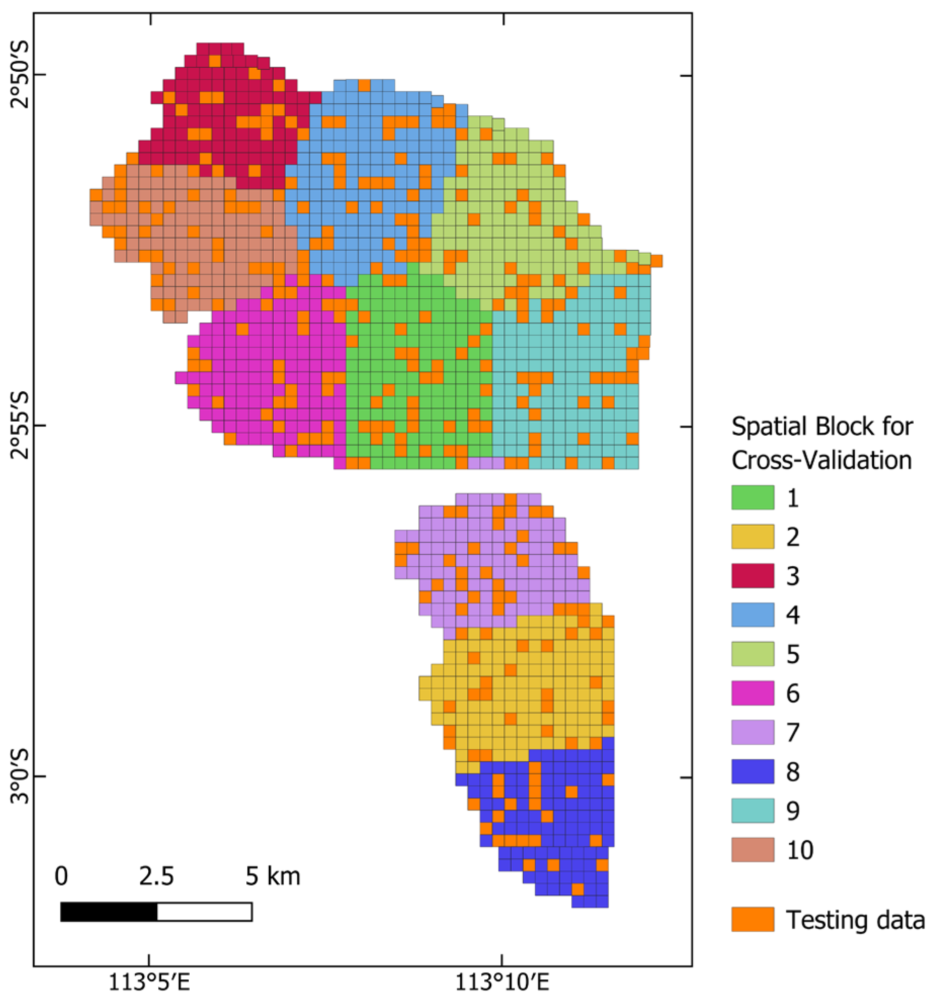
The training entails 1266 patches, or 80% of the total datasets. The accuracy was then assessed by calculating the errors on the remaining 20% of the datasets. In addition, we evaluated the model training by performing spatial block cross-validation (CV) using k-means clustering based on the centroid of training patch datasets. The training patches were clustered into 10 spatial folds (see Figure A2). After training, the model inference was carried out on the entire study area, which was split into patches of size 2048 × 2048 pixels with some overlapped areas. To avoid edge artifacts, we trimmed 16 pixels in the image boundaries and filled them with overlapped patches.

In the next stage, we employed power-law regression to produce a wall-to-wall AGB map. Several studies have reported that a single variable of CHM can predict AGB through regression analysis [30,43]. Here, we used DL-based CHM as the independent variable and plot-based field AGB data as the dependent variable. Considering the larger extent of forest inventory plots than the pixel size of the CHM map, mean values were calculated on pixels that fall into each corresponding field plot.

3.4.2. StepwiseReg-DL Model

This second approach involves (1) LiDAR-based AGB mapping in the partial area and (2) a DL-based upscaling method to the whole study area. The stepwise regression was applied on the LiDAR metrics using the dependent variable of ground truth AGB data to derive an AGB map in the area covered by LiDAR.

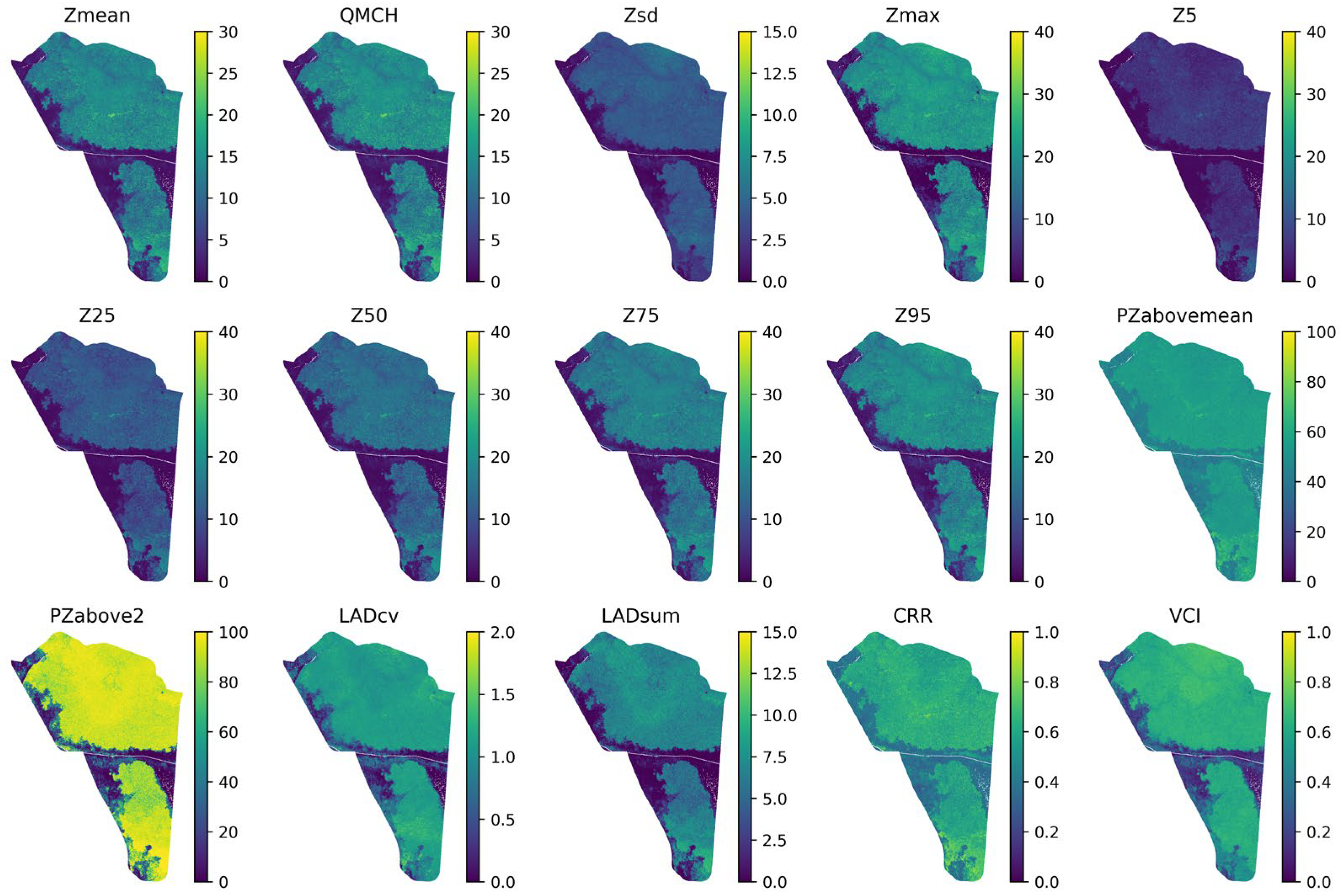
First, LiDAR metrics were obtained using the lidR package on R studio [44]. The non-ground points were normalized based on the elevation values of DTM. We calculated 15 LiDAR-derived metrics as shown in Figure A3 describing canopy height, canopy arrangement, leaf area density, and canopy cover [45]. Height metrics included the mean (Zmean), quadratic mean canopy height (QMCH), standard deviation (Zsd), maximum (Zmax), and height percentiles (Z5, Z25, Z50, Z75, Z95). Canopy arrangement was characterized using the canopy relief ratio (CRR) and vertical complexity index (VCI). Leaf area density was represented by the total leaf area density (LADsum) and the coefficient of variation of leaf area density (LADcv) [46]. Finally, canopy cover was quantified using the proportion of returns above mean height (PZabovemean) and above 2 m (PZabove2).

In the second step, we applied a stepwise AIC (Akaike information criterion) method for variable selection in linear regression, meaning that the variables are iteratively added or removed to find the best-suited model with the lowest AIC [47]. Once the variables were selected, the OLS (ordinary least squares) algorithm was employed to estimate the relationship between AGB and selected LiDAR metrics. The regression equation was then used to predict AGB in this southern part of the study area.

The wall-to-wall AGB map in this workflow was conducted by the DL method, adopting the same architecture to predict CHM in the previous section. The difference was the input data, which used log-transformed LiDAR-based AGB patches generated from stepwise regression. In addition, an early stop strategy was also implemented due to indications of overfitting during training. This early stopping strategy based on the validation loss was employed to terminate training when no further improvement was observed. The accuracy of the final AGB map was assessed using the same validation set in the DL-PowerReg model.

4. Results

4.1. DL-PowerReg: CHM

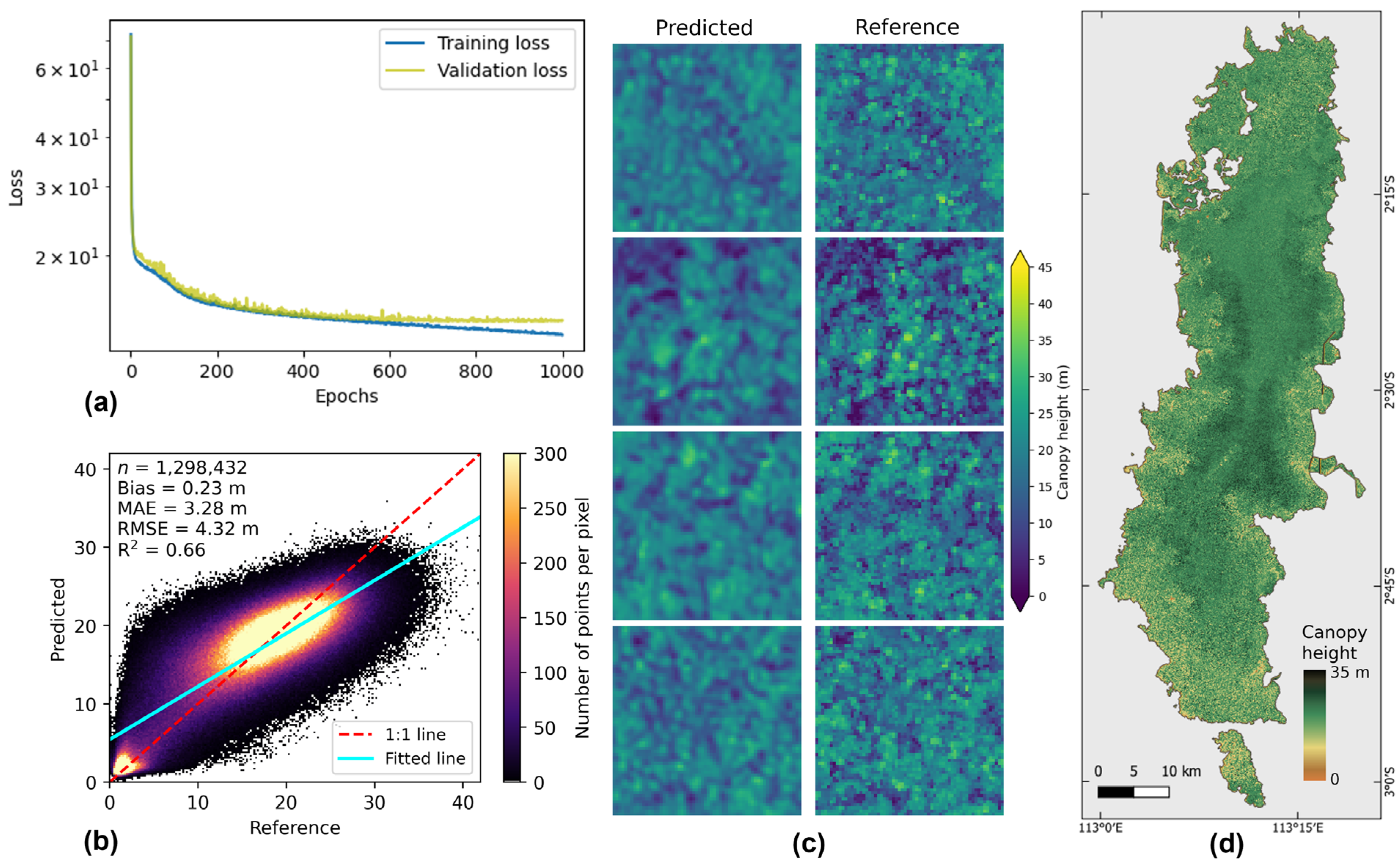
CHM of the entire study area was predicted using a U-Net-based deep learning model trained on four-band Planet imagery. The model was trained over 1000 epochs across the complete dataset. This epoch count was determined by referring to the similar study in Wagner et al. [23] and through preliminary experiments to minimize overfitting, as validation loss showed no further improvement beyond this point (Figure 5a). Based on the testing datasets, the model achieved a prediction MAE of 3.23 m, while the spatial block CV reported a mean MAE of 3.54 ± 0.32 m. Although the predictions did not perfectly follow the 1:1 line, they remained comparable to the reference CHM data (Figure 5b). As shown in Figure 5c, the model broadly captured the spatial patterns of CHM across the study area. However, the predicted canopy texture appeared smoother than that of the very-high-resolution LiDAR reference data, which resulted in a loss of fine-scale tree structural detail, particularly at extreme height values, although crown shapes remained discernible owing to the 5 m spatial resolution of the output. The CHM map indicated that the peat swamp forest had a mean canopy height of 20.22 m, with the 25th and 75th percentiles at 18.42 m and 22.63 m, respectively.

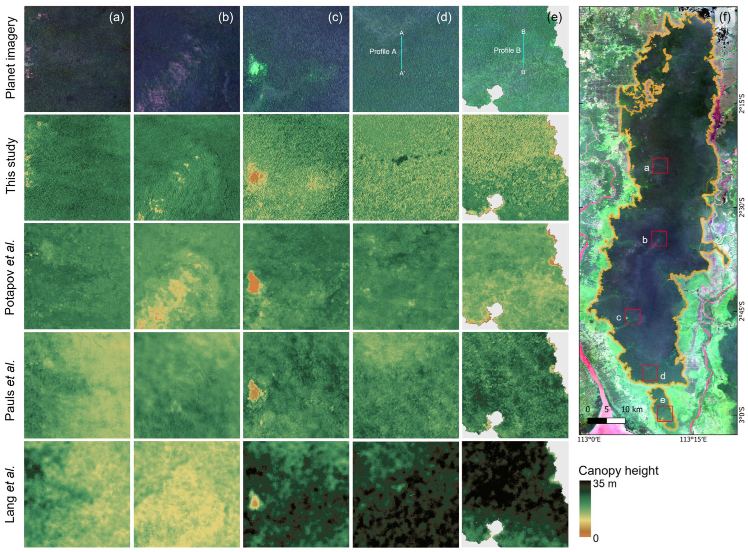
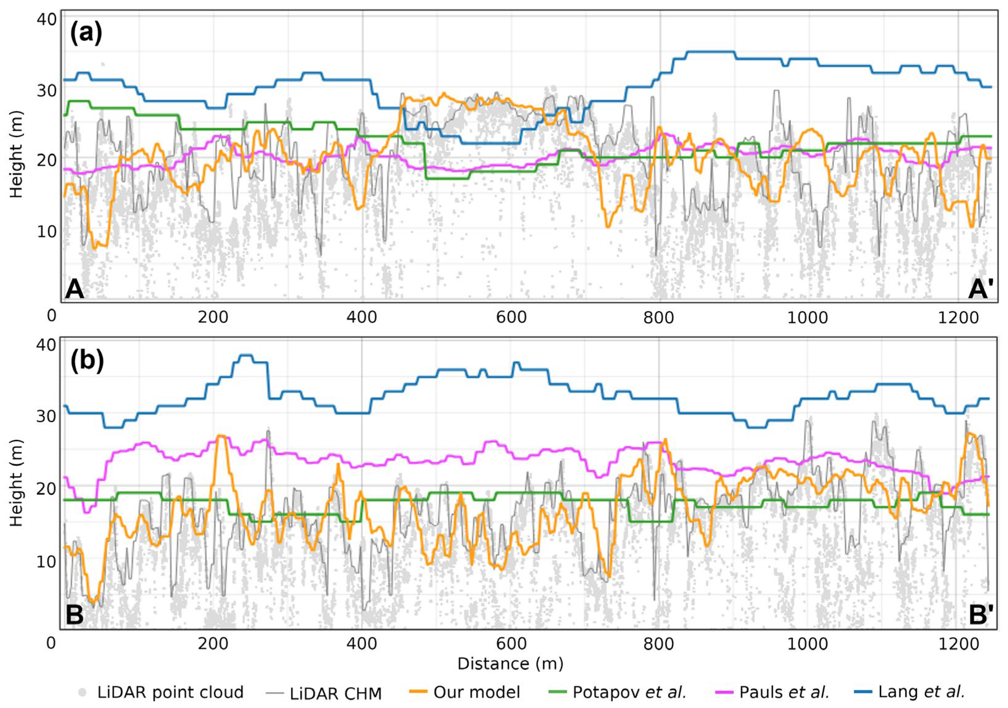
As global datasets of CHM are publicly available, our CHM estimates were evaluated against three models from Potapov et al. [19], Pauls et al. [48], and Lang et al. [18]. Figure 6 presents side-by-side comparisons of these CHM models alongside Planet imagery across five subset areas. As shown in Figure 6c, all models were capable of detecting deforestation patches; however, canopy height distributions varied considerably within the forested areas. The models by Pauls et al. [48] and Lang et al. [18] underestimated the height of tall, undisturbed forest (Figure 6a) and failed to clearly distinguish the low-stature pole peat swamp forest (Figure 6b). Among the global datasets, Potapov et al. [19] showed the most similar spatial patterns to our estimates, with the exception of subset (e), where their model mapped shorter trees in the southern area, which is contrary to our results. Overall, the dataset from Potapov et al. [19] was the closest to both the LiDAR reference and our model, whereas the remaining datasets showed a general tendency toward overestimation (Figure 6e and Figure 7b).

The regrowth area in Figure 6d (also shown in Figure 7a) was accurately estimated only by our model. The global datasets, which were predominantly derived from optical sensors, predicted this area to have shorter trees, likely because the low canopy reflectance captured by Planet imagery was misinterpreted as low vegetation. In this study, the combination of high-resolution Planet imagery and the U-Net architecture enabled the model to learn the textural characteristics of the regrowth area effectively, resulting in more accurate height estimates.

4.2. DL-PowerReg: Final AGB Map

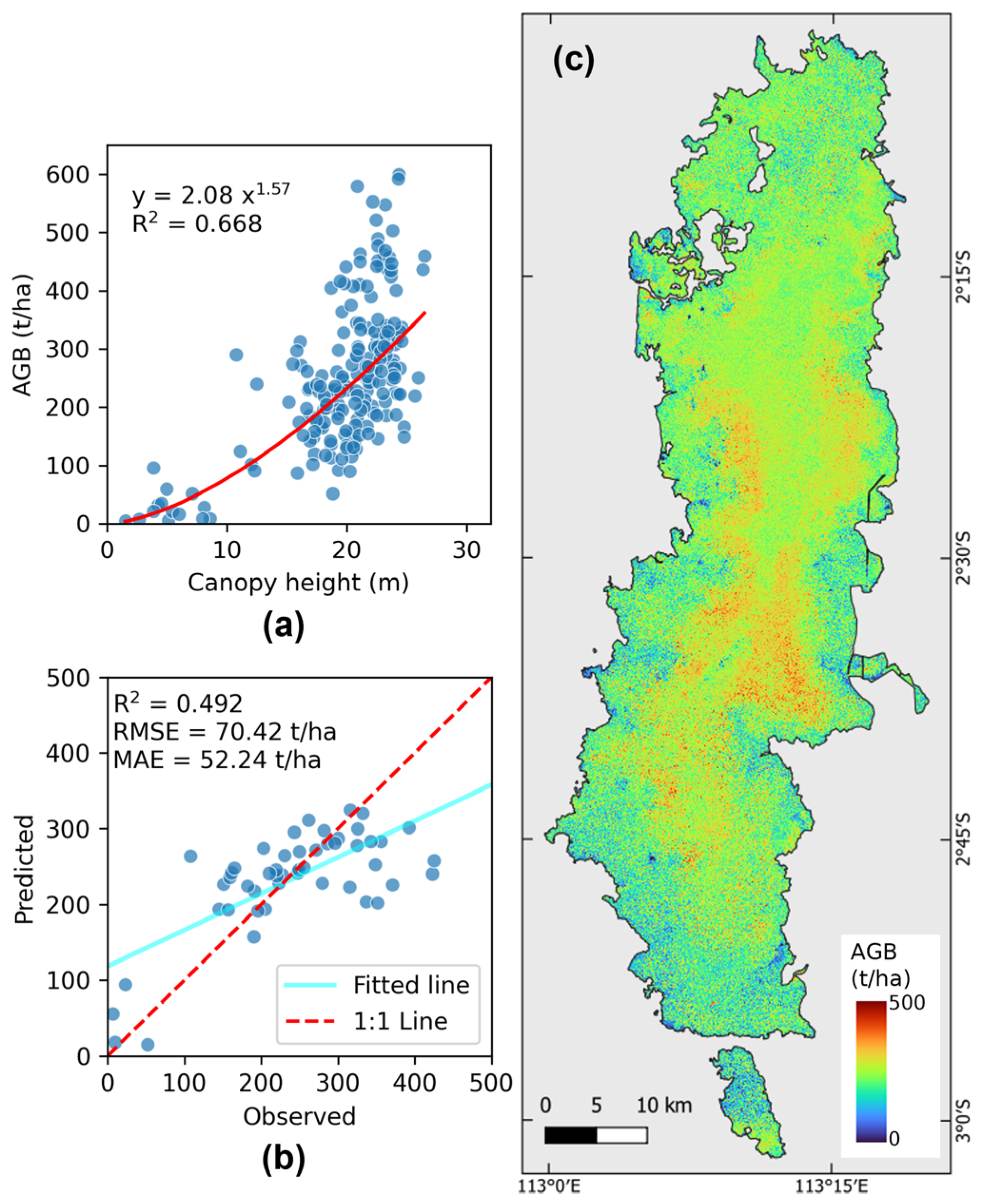
To generate an AGB map of the study area, power regression was applied with ground truth data as the dependent variable and DL-based CHM as the independent variable. The regression achieved an R² of 0.67, indicating that 67% of the variance in AGB can be explained by the CHM product. Figure 8a revealed the predictive relationship between canopy height and AGB weakened at canopy heights above approximately 22 m. Although the fitted power function continued to increase with CHM, the variability in AGB became substantially larger for stands with similar canopy heights. This indicates that CHM alone was insufficient to discriminate among high-biomass stands, where biomass accumulation is increasingly governed by stem diameter, basal area, wood density, and canopy structural complexity rather than further increases in dominant canopy height. Consequently, some high biomass values were underestimated, as reflected in the accuracy assessment. Overall, the model yielded an MAE of 52.24 t/ha, an RMSE of 70.42 t/ha, and an R² of 0.49. The final AGB map produced by this approach estimated a total AGB of 47.75 Mt across the study area, with a mean value of 239.91 t/ha.

4.3. StepwiseReg-DL: LiDAR-Based AGB

The AIC stepwise method selected two input variables for the multiple linear regression: QMCH and PZabovemean. The regression equation is as follows:

$$AGB=14.682+(QMCH\times 24.428)+(PZabovemean\times -3.694)$$

(3)

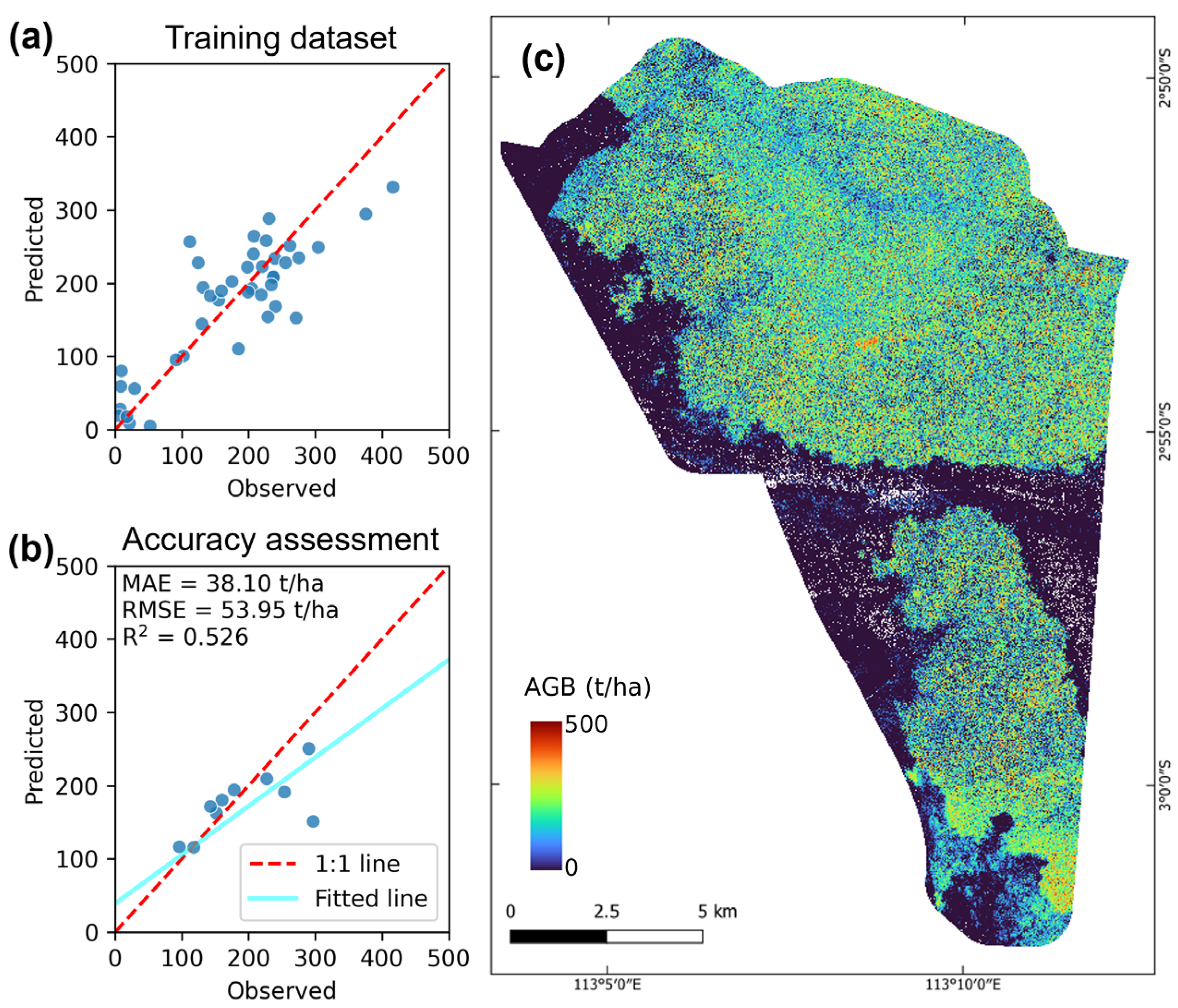
where AGB, QMCH, and PZabovemean denote aboveground biomass at 5 m pixel size, quadratic mean canopy height, and proportion of returns above mean, respectively. The regression model achieved an R² of 0.72 (Figure 9). Accuracy assessment on independent samples reported an MAE of 38.10 t/ha and an R² of 0.53. The derived regression equation was subsequently applied to the selected LiDAR metrics to generate an AGB map for the southern area covered by LiDAR data.

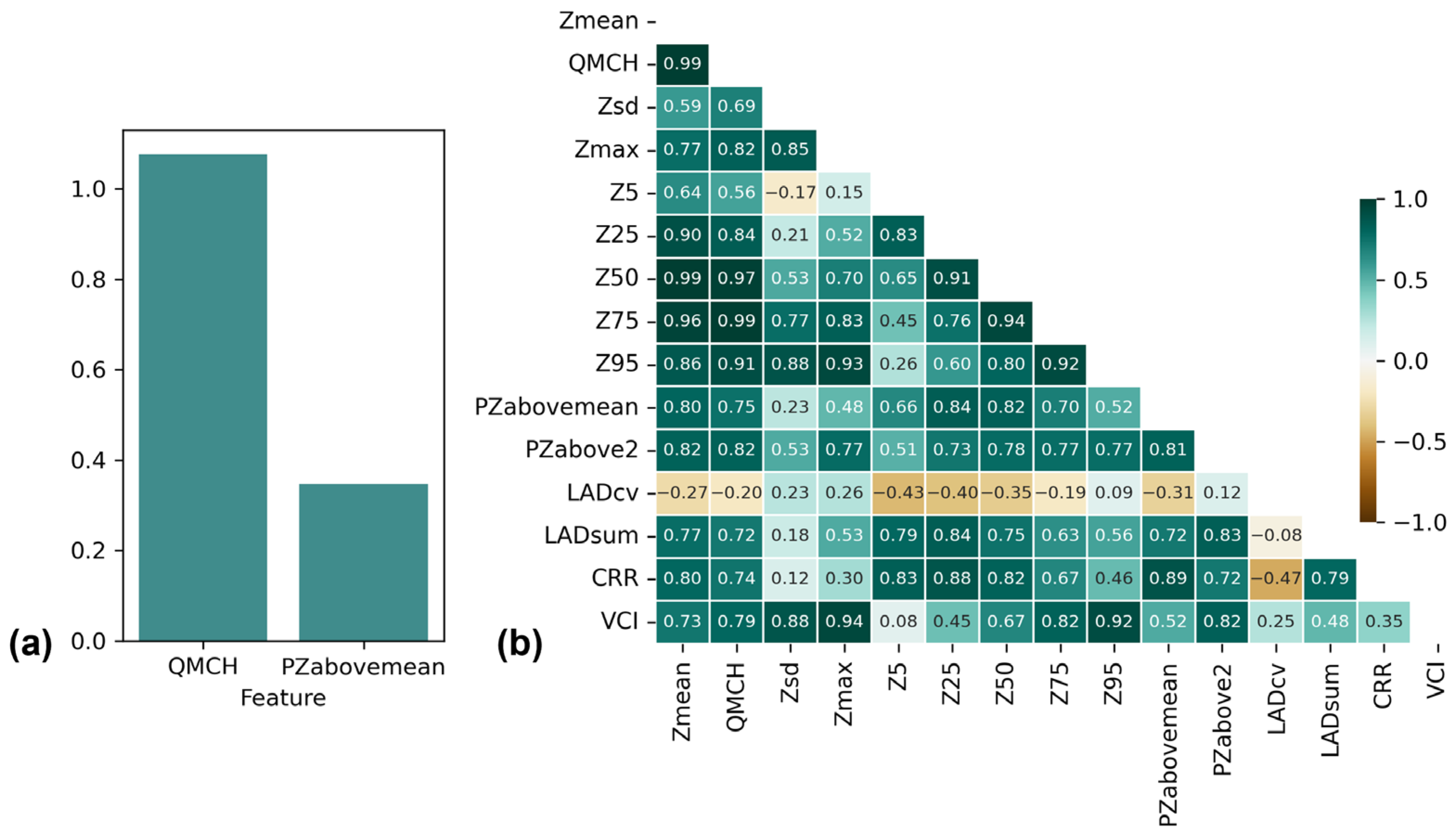
The stepwise regression retained two variables while excluding the remaining 13 point cloud metrics. Figure 10 illustrated the pairwise correlations among the LiDAR metrics considered as candidate inputs. Height metrics were generally strongly correlated with one another, with the exception of height variation and the lower quantile, represented by Zsd and Z5. QMCH emerged as the most important predictor, capturing the vertical structure of the canopy through its strong associations with Zmean and height quantiles from Z25 upward. QMCH also showed strong correlations (r > 0.7) with metrics related to canopy arrangement, leaf area density, and canopy cover, except for LADcv. The second selected variable, PZabovemean, characterized horizontal canopy cover. Together, the two variables incorporated both the vertical and horizontal structural dimensions of the forest as derived from LiDAR point clouds. In addition, QMCH and PZabovemean exhibited a moderate positive correlation (r = 0.75). To assess potential multicollinearity in the regression model, variance inflation factors (VIFs) were calculated. Both predictors had a VIF of 2.28 (VIF < 5), indicating that multicollinearity is not significant in the final model [49].

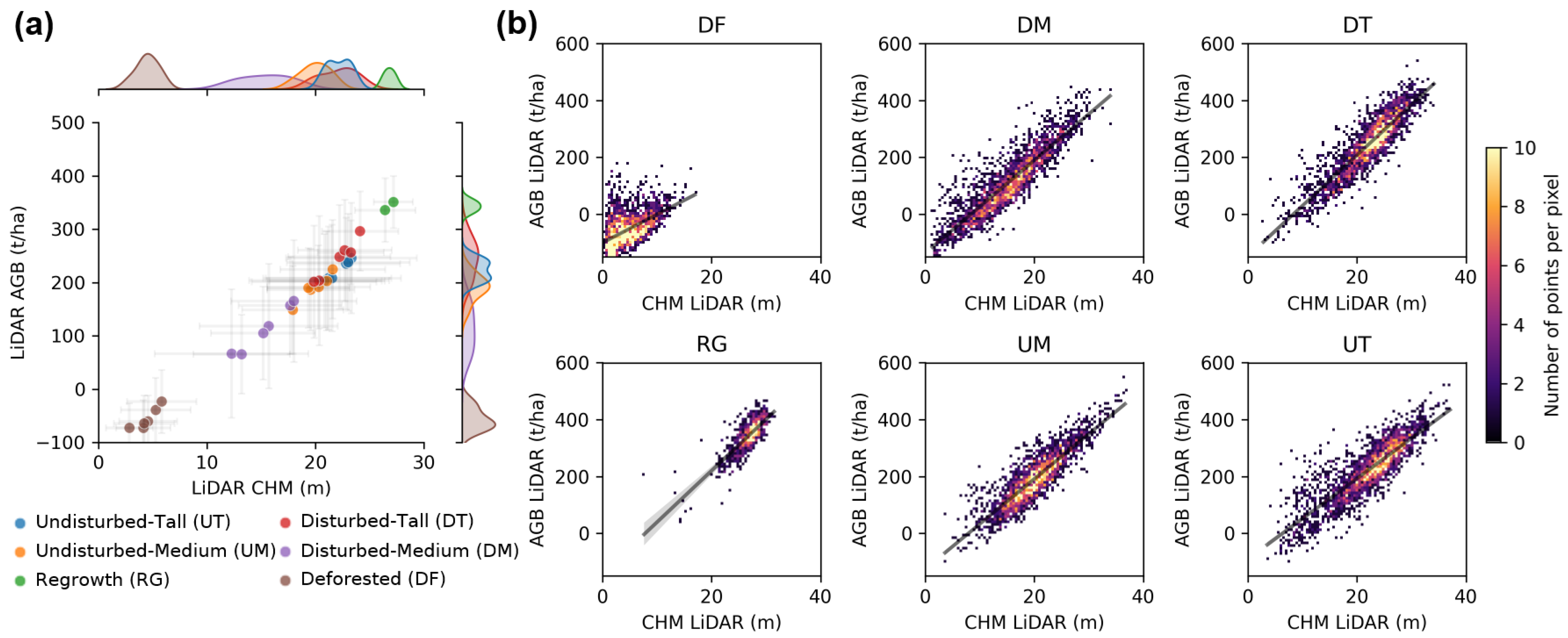
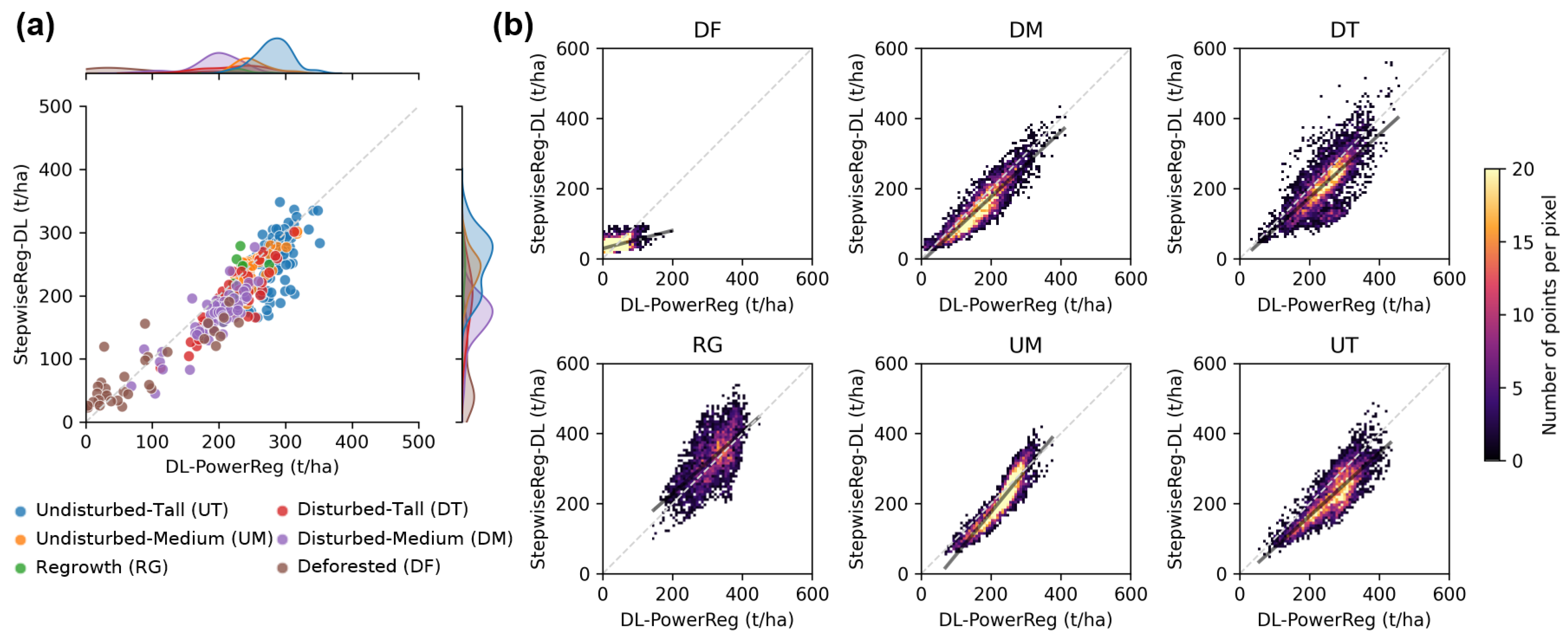
The AGB estimates from the stepwise regression with LiDAR CHM were compared across six forest condition and height categories: deforested (DF), regrowth (RG), disturbed-medium (DM), disturbed-tall (DT), undisturbed-medium (UM), and undisturbed-tall (UT). Raster values were extracted from 1 ha random plots within each class (Figure A4). Figure 11 showed a consistent linear relationship between AGB and tree height across all classes, with similar gradients, except in the deforested class. Negative AGB values were found in low-CHM areas, predominantly in deforested and disturbed-medium zones, due to the exclusion of non-forest plots from the regression analysis. Since the analysis focused on standing AGB, values below zero were masked in the subsequent step as they corresponded to non-tree objects; thus, the negative values did not affect the model training.

4.4. StepwiseReg-DL: Final AGB Map

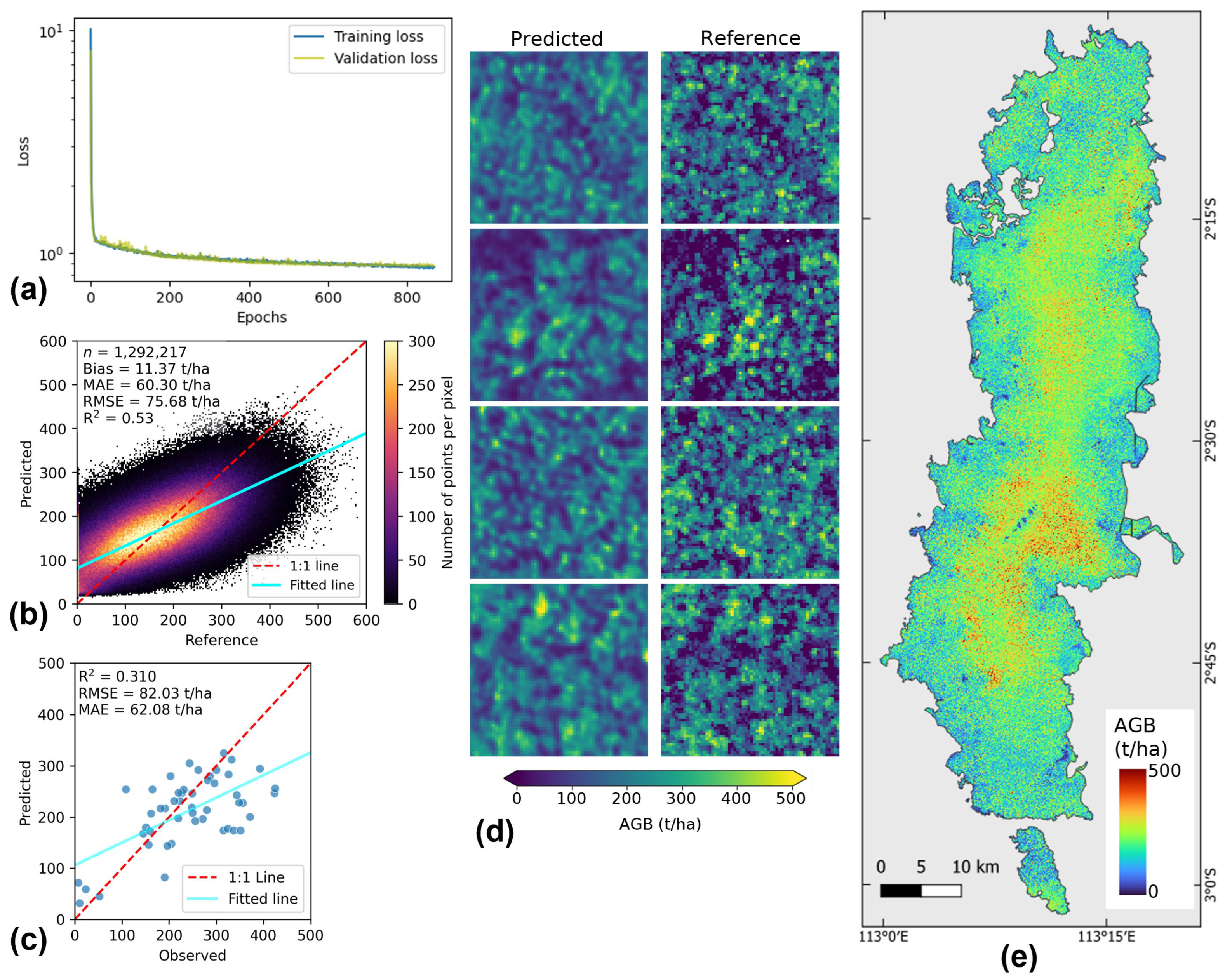
The U-Net deep learning model in this approach used LiDAR-derived AGB from the stepwise regression as a reference and four-band Planet imagery as input. The architecture followed the same design as in the CHM modeling of DL-PowerReg; however, early stopping was applied to limit the number of training epochs and mitigate overfitting. The model converged after 868 epochs (Figure 12a). The evaluation using separate image patches from training datasets revealed a tendency toward underestimation at high biomass values and overestimation at very low biomass values. While the model testing exhibited an MAE of 60.30 t/ha, the spatial block CV showed a lower accuracy with a mean MAE of 64.92 ± 8.79 t/ha. As shown in Figure 12d, the spatial predictions were smoother than the reference images, consistent with the pattern observed in the CHM model evaluation of DL-PowerReg. Accuracy was assessed using the same validation dataset as in the DL-PowerReg approach. The final AGB map of the StepwiseReg-DL method yielded an MAE of 62.08 t/ha, an RMSE of 82.03 t/ha, and an R² of 0.31. The lower R² reflected greater dispersion around the 1:1 line and compression of the predicted biomass range, and it showed a lower ability of the model to capture the variability of high-biomass stands. This approach estimated a total AGB of 40.07 Mt with an average of 201.30 t/ha.

4.5. Approach Comparison

We compared the validation samples of DL-PowerReg and StepwiseReg-DL methods. Additionally, several random 1 ha plots were also extracted to see the differences across forest classes (Figure A4). Overall, both methods produced moderately similar results (Figure 13). At the forest class level, both approaches yielded comparable AGB estimates for disturbed-medium, disturbed-tall, undisturbed-medium, and undisturbed-tall peat swamp forests. StepwiseReg-DL tended to underestimate AGB in the deforested class while producing higher estimates in regrowth forests relative to DL-PowerReg.

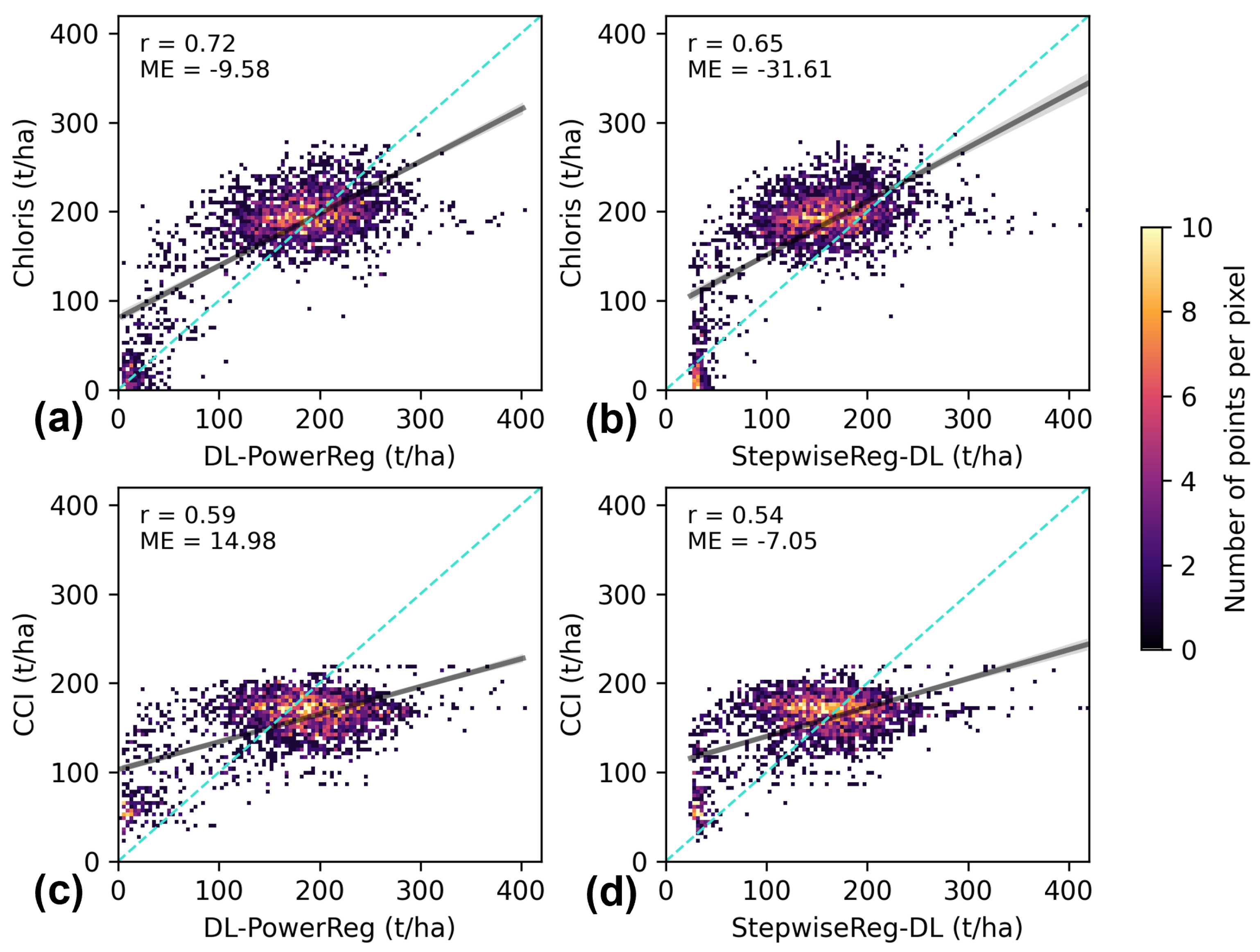
A comparison was also conducted with two global AGB products: ESA’s CCI Biomass [50] and Chloris [51]. CCI Biomass 2022 was used at its native spatial resolution of 100 m and is freely accessible. Chloris AGB (30 m resolution), while not publicly available, was included in the comparison as it is derived from regional-based models. Due to the limited spatial coverage of the Chloris product, only 211 ha was analyzed. Both our AGB maps and the Chloris product were resampled to 100 m to match the resolution of ESA CCI Biomass. Figure 14 showed that both global datasets exhibited saturation relative to our AGB maps. Chloris showed obvious saturation at high biomass values, while CCI Biomass struggled to capture high biomass, as indicated by its narrow value range. Our AGB maps showed moderate correlations with the Chloris dataset (r = 0.72 and 0.65) yet demonstrated a greater capacity to detect higher biomass values.

5. Discussion

The DL-PowerReg approach produced an intermediate result in the form of a CHM map covering the entire study area through a U-Net deep learning model trained on Planet NICFI imagery. This CHM product achieved an MAE of 3.23 m (MAE of spatial block CV = 3.54 ± 0.32 m) at 5 m spatial resolution, capturing canopy height variation down to the crown level. The accuracy of our CHM model surpassed that of the global datasets, such as Potapov et al. [19], Pauls et al. [48], and Lang et al. [18] which reported an MAE of 4.45, 4.45 (trees > 5 m), and 4.00 m, respectively. Our model also outperformed Wagner et al. [23], which reported an MAE of 3.68 m for CHM prediction in the Amazon forest using a comparable workflow. The present study additionally addressed a gap left by Pickstone et al. [52], who applied the same LiDAR reference data in Katingan–Mentaya but adopted a different modeling strategy. They used eight-band Planet imagery incorporated with topographic and vegetation indices. Their best results were achieved with a random forest model at 3 m and 10 m resolutions, yielding MAEs of 4.27 m and 3.01 m, respectively. By only using four spectral bands (RGB-NIR) from Planet NICFI imagery, our model exhibited better accuracy than their very-high-resolution Planet-based CHM product, yet it showed slightly poorer accuracy than their 10 m model. This confirmed the advantages of CNN-based architectures such as U-Net in learning vegetation structural properties through iterative spatial feature extraction, even when spectral input is limited [34].

Based on the final biomass accuracy assessment, the DL-PowerReg model (MAE = 52.24 t/ha) outperformed the StepwiseReg-DL model (MAE = 62.08 t/ha) by a margin of 9.84 t/ha. The lower coefficient of determination of the StepwiseReg-DL (R² = 0.31) also indicates that it explained substantially less of the observed biomass variability than the DL-PowerReg model (R² = 0.49). Despite this difference, scatterplots of predicted versus observed AGB showed that both models performed reasonably well at low-to-medium biomass values but struggled at the higher end of the distribution, where a systematic underestimation was observed. First, the underestimation of high AGB values is partly attributable to the imbalanced distribution of the reference data used for U-Net training [36]. Although a weighted loss function was adopted to mitigate this imbalance, underprediction of the relatively few high-biomass samples remained unavoidable. Second, canopy height became a less effective predictor of AGB above approximately 22 m (Figure 8a). While AGB generally increased with CHM, the dispersion of AGB values increased markedly at taller canopies, indicating that forests with similar canopy heights could possess substantially different biomass. As a result, the power regression based solely on CHM was unable to adequately distinguish high-biomass stands.

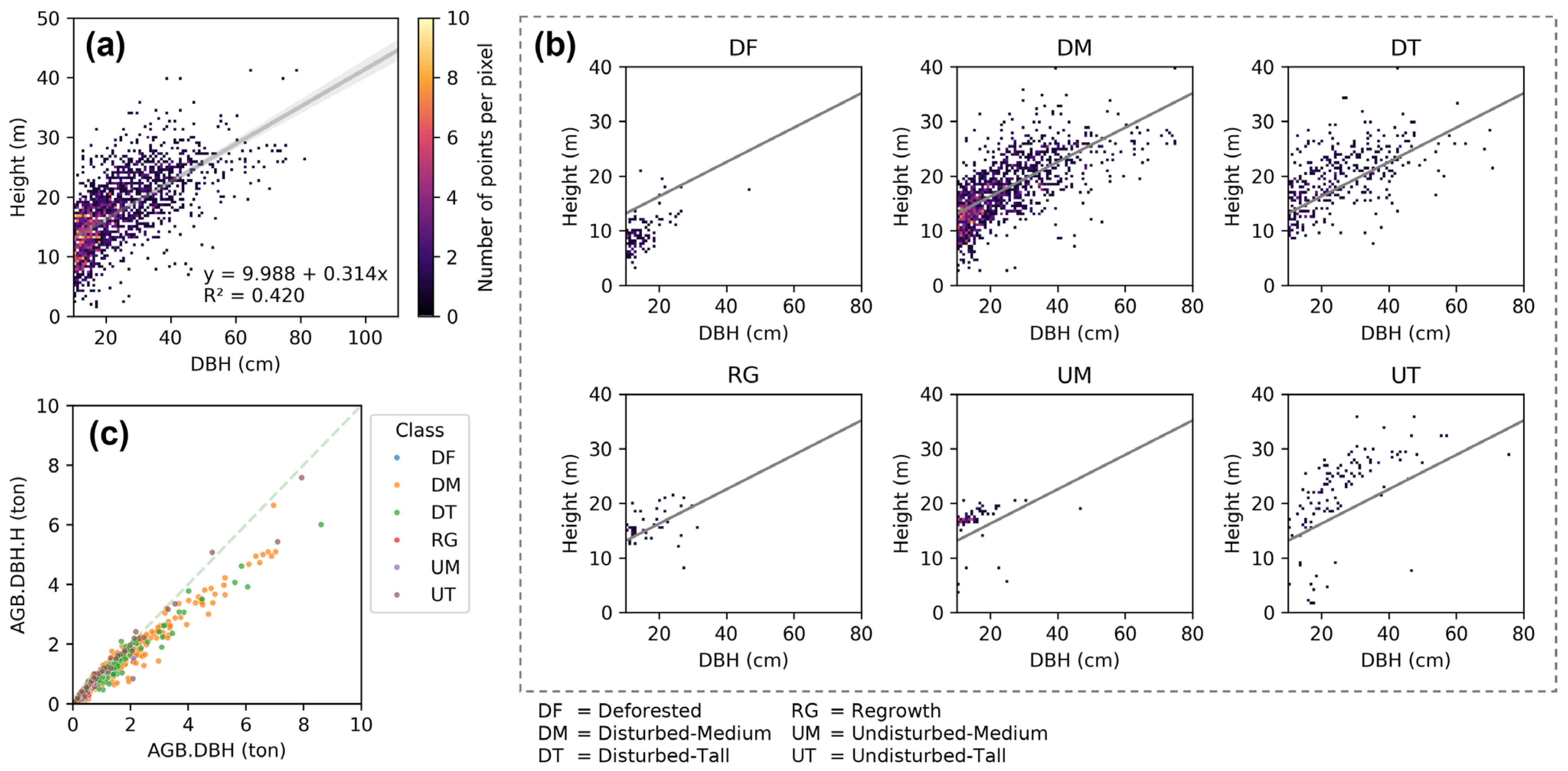
This limitation was further compounded by uncertainties in the forest inventory data used as a reference. Due to the very limited number of plots with tree height measurements, the in situ AGB data were derived from an allometric equation considering only DBH. As shown in Figure A5, tree height exhibited saturation in inventory plots with complete measurements once trees exceeded approximately 50 cm in DBH, indicating that height increased only marginally despite continued stem growth. Consequently, allometric equations relying solely on DBH produced higher AGB estimates than equations incorporating both DBH and tree height. Although many forest inventories rely exclusively on DBH measurements, DBH-only allometric models have been reported to overestimate biomass in mature forests [53]. The uncertainty in the reference AGB therefore further constrained the model’s ability to resolve high-biomass conditions.

To improve predictions, future studies could explore a broader set of variables that better represent complex canopy structures. The LiDAR-based AGB estimates in this study suggested that horizontal canopy structure, alongside vertical metrics, contributed meaningfully to AGB variation. For instance, canopy density could be incorporated as an additional predictor in the DL-PowerReg workflow, rather than relying on CHM alone. In addition, enriching the candidate variable pool in LiDAR-based AGB modeling with plot-level basal area and basal-area-weighted wood density could further improve predictions [54], although implementation at landscape scale remains challenging due to the requirement for spatially continuous wood density data.

Despite the underestimation at high biomass values reported in this study, both Chloris and CCI Biomass global datasets exhibited even greater saturation relative to our AGB maps (Figure 14). These global products were generated using models trained across broad geographic extents. Although region- or biome-specific implementations were applied, such as in Chloris, potential biases remained for ecosystems with high structural diversity. In contrast, our model was built specifically for the peatland ecosystem of the study area, which likely contributed to more precise local predictions but inherently limited its transferability to broader regions.

The DL-PowerReg model produced higher AGB estimates than StepwiseReg-DL. The lower estimates from StepwiseReg-DL were attributed to the limited spatial distribution of the reference data used for AGB upscaling through U-Net. The LiDAR-based AGB derived from stepwise regression covered only the southern part of the study area, which, as shown in Figure 12, had relatively lower AGB than the rest of the study area. Similarly, the ground truth data used for model training were also lower compared to those of DL-PowerReg and validation (Figure A1). This introduced a geographic bias into the training data. Moreover, the U-Net model consequently learned from a sample space dominated by low-to-medium biomass values, which limited its ability to generalize to higher-biomass conditions. On the other hand, the power regression step in DL-PowerReg used more spatially distributed samples across the Katingan–Mentaya area, despite a smaller total sample size (n = 197). The broader spatial coverage allowed the model to better represent the full range of AGB variation across the study area. StepwiseReg-DL benefited from richer structural information provided by LiDAR metrics and a larger number of U-Net training samples, yet its reference data suffered from spatial imbalance. This limited its ability to outperform DL-PowerReg, particularly at higher biomass values. These findings highlight the importance of sample spatial distribution in AGB modeling. In cases where LiDAR data is available only for a limited portion of the mapping area, as in this study, we recommend the DL-PowerReg approach, because it is less sensitive to spatial imbalance in the reference data and additionally provides a CHM product that supports broader forest condition assessments.

Based on the final AGB maps and by incorporating bootstrap uncertainty analysis (Appendix B), the DL-PowerReg model estimated a total AGB of 47.75 Mt (mean = 239.91 t/ha; 95% bootstrap CI: 44.01–52.13 Mt), whereas the StepwiseReg-DL model estimated 40.07 Mt (mean = 201.30 t/ha; 95% bootstrap CI: 35.95–44.40 Mt). The bootstrap distribution of the difference between the two estimates had a mean of 7.71 Mt (95% CI: 5.99–9.19 Mt), which did not include zero, indicating that the difference between the two methods was statistically significant under the bootstrap framework. Our estimates based on both approaches exceeded those reported by PT RMU (unpublished), which recorded an average AGB of 149.7 ± 61.27 t/ha based on 30 m mapping using the integration of GEDI, Sentinel-1, Sentinel-2, and Chloris biomass. The discrepancies likely reflect differences in estimation approaches and the spatial extent of the assessed areas (i.e., the project area versus the peat hydrological unit).

The forest class samples presented in Figure 13 showed mean AGB values of 249.31 t/ha and 219.72 t/ha in undisturbed peat swamp forests and 207.92 t/ha and 181.78 t/ha in disturbed forests for DL-PowerReg and StepwiseReg-DL, respectively. These values are consistent with the ranges reported by Verwer and van der Meer [55], who summarized that undisturbed peat swamp forest stored 147–645 t/ha (noting that the upper bound of 645 t/ha was recorded from a single tall interior forest plot by Waldes and Page [56]), while logged and degraded peat swamp forest ranged from 130 to 334 t/ha. Notably, natural regrowth forests within the disturbed peat swamp forest class showed high mean AGB values of 316.50 t/ha (DL-PowerReg) and 331.64 t/ha (StepwiseReg-DL). These high values indicate the positive impact of conservation measures in the area. Katingan–Mentaya was formerly a forest concession area subject to selective logging, where most extensive disturbances were in the southern part. The permit was withdrawn in 2000, and since then, illegal logging by local communities has been reported, although it has shown a declining trend in recent years.

Given the importance of high-resolution AGB mapping for monitoring conservation and restoration progress in peat swamp forests, continued mapping efforts are strongly recommended. To replicate this study in the same area, model inference for both workflows would require Planet imagery with the same sensor specifications and pre-processing steps. Temporal transferability of such models has been demonstrated by previous studies; however, consistent input data characteristics are a prerequisite to avoid introducing systematic bias into predictions [57]. Nevertheless, validation data would still be required, particularly at the same inventory plots, to confirm monitoring assessments. In addition, new LiDAR surveys, although costly, could further improve model performance by retraining the existing models with updated datasets.

The spatial transferability of the developed models to other forest types should be considered with caution. Since both models were developed specifically for the Katingan–Mentaya peat swamp forest, their predictive relationships are likely influenced by the structural characteristics, species composition, and biomass distribution of this ecosystem. Applying the models directly to forests with different characteristics may reduce prediction accuracy, and recalibration or retraining using representative local reference data would likely be required. Furthermore, although the U-Net architecture itself can be adapted to higher-resolution multispectral satellite data from other sensors, model performance would depend on differences in spatial resolution, spectral band configuration, radiometric characteristics, and pre-processing procedures. Consequently, transferring a trained model directly across sensors is unlikely to achieve optimal performance without data harmonization and subsequent retraining or fine-tuning. Future studies should evaluate the robustness of both modeling approaches across a wider range of forest types and satellite platforms to improve their operational applicability.

6. Conclusions

This study demonstrated two workflows, i.e., DL-PowerReg and StepwiseReg-DL, for estimating forest biomass using high-resolution Planet imagery combined with spatially incomplete airborne LiDAR data. DL-PowerReg (MAE = 52.24 t/ha) outperformed StepwiseReg-DL (MAE = 62.08 t/ha), primarily due to the more spatially distributed ground truth data used for the final AGB estimation. The reference data used for upscaling in StepwiseReg-DL was limited only in the southern portion of the study area, which introduced geographic bias despite the larger sample size. By leveraging an accurate intermediate CHM product (MAE = 3.23 m), DL-PowerReg provided information on both forest structure and biomass storage, offering a more comprehensive characterization of forest conditions. The final AGB maps estimated total standing biomass in the Katingan–Mentaya peat swamp forest at 47.75 Mt (mean = 239.91 t/ha) for DL-PowerReg and 40.07 Mt (mean = 201.30 t/ha) for StepwiseReg-DL. These findings demonstrate that Planet imagery can effectively complement spatially limited LiDAR data for wall-to-wall forest biomass assessments. Continued high-resolution mapping is recommended to monitor conservation and restoration progress in tropical peat swamp forests.

References

1. Mitchard, E.T.A. The Tropical Forest Carbon Cycle and Climate Change. Nature 2018, 559, 527–534. [Google Scholar] [CrossRef] [Scilit] [PubMed]
2. Pan, Y.; Birdsey, R.A.; Phillips, O.L.; Houghton, R.A.; Fang, J.; Kauppi, P.E.; Keith, H.; Kurz, W.A.; Ito, A.; Lewis, S.L.; et al. The Enduring World Forest Carbon Sink. Nature 2024, 631, 563–569. [Google Scholar] [CrossRef] [Scilit] [PubMed]
3. Santoro, M.; Cartus, O.; Carvalhais, N.; Rozendaal, D.M.A.; Avitabile, V.; Araza, A.; De Bruin, S.; Herold, M.; Quegan, S.; Rodríguez-Veiga, P.; et al. The Global Forest Above-Ground Biomass Pool for 2010 Estimated from High-Resolution Satellite Observations. Earth Syst. Sci. Data 2021, 13, 3927–3950. [Google Scholar] [CrossRef] [Scilit]
4. Jaenicke, J.; Rieley, J.O.; Mott, C.; Kimman, P.; Siegert, F. Determination of the Amount of Carbon Stored in Indonesian Peatlands. Geoderma 2008, 147, 151–158. [Google Scholar] [CrossRef] [Scilit]
5. Page, S.E.; Rieley, J.O.; Banks, C.J. Global and Regional Importance of the Tropical Peatland Carbon Pool. Glob. Change Biol. 2011, 17, 798–818. [Google Scholar] [CrossRef] [Scilit]
6. Miettinen, J.; Shi, C.; Liew, S.C. Land Cover Distribution in the Peatlands of Peninsular Malaysia, Sumatra and Borneo in 2015 with Changes since 1990. Glob. Ecol. Conserv. 2016, 6, 67–78. [Google Scholar] [CrossRef] [Scilit]
7. Konecny, K.; Ballhorn, U.; Navratil, P.; Jubanski, J.; Page, S.E.; Tansey, K.; Hooijer, A.; Vernimmen, R.; Siegert, F. Variable Carbon Losses from Recurrent Fires in Drained Tropical Peatlands. Glob. Change Biol. 2016, 22, 1469–1480. [Google Scholar] [CrossRef] [Scilit] [PubMed]
8. Osaki, M.; Kato, T.; Kohyama, T.; Takahashi, H.; Haraguchi, A.; Yabe, K.; Tsuji, N.; Shiodera, S.; Rahajoe, J.S.; Atikah, T.D.; et al. Basic Information About Tropical Peatland Ecosystems. In Tropical Peatland Eco-Management; Osaki, M., Tsuji, N., Foead, N., Rieley, J., Eds.; Springer: Singapore, 2021; pp. 3–62. [Google Scholar]
9. Nurbaya, S. FOLU NET SINK: Indonesia’s Climate Actions Towards 2030; The Ministry of Environment and Forestry of the Republic of Indonesia: Jakarta, Indonesia, 2023.
10. Harrison, R.D.; Swinfield, T.; Ayat, A.; Dewi, S.; Silalahi, M.; Heriansyah, I. Restoration Concessions: A Second Lease on Life for Beleaguered Tropical Forests? Front. Ecol. Environ. 2020, 18, 567–575. [Google Scholar] [CrossRef] [Scilit]
11. Darusman, T.; Lestari, D.P.; Arriyadi, D. Management Practice and Restoration of the Peat Swamp Forest in Katingan-Mentaya, Indonesia. In Tropical Peatland Eco-Management; Osaki, M., Tsuji, N., Foead, N., Rieley, J., Eds.; Springer: Singapore, 2021; pp. 381–409. [Google Scholar]
12. Barbosa, J.M.; Broadbent, E.N.; Bitencourt, M.D. Remote Sensing of Aboveground Biomass in Tropical Secondary Forests: A Review. Int. J. For. Res. 2014, 2014, 715796. [Google Scholar] [CrossRef] [Scilit]
13. Camarretta, N.; Harrison, P.A.; Bailey, T.; Potts, B.; Lucieer, A.; Davidson, N.; Hunt, M. Monitoring Forest Structure to Guide Adaptive Management of Forest Restoration: A Review of Remote Sensing Approaches. New For. 2020, 51, 573–596. [Google Scholar] [CrossRef] [Scilit]
14. Mazlan, S.M.; Wan Mohd Jaafar, W.S.; Muhmad Kamarulzaman, A.M.; Saad, S.N.M.; Mohd Ghazali, N.; Adrah, E.; Abdul Maulud, K.N.; Omar, H.; Teh, Y.A.; Dzulkifli, D.; et al. A Review on the Use of LiDAR Remote Sensing for Forest Landscape Restoration. In Concepts and Applications of Remote Sensing in Forestry; Suratman, M.N., Ed.; Springer Nature: Singapore, 2022; pp. 49–74. [Google Scholar]
15. Alvites, C.; Marchetti, M.; Lasserre, B.; Santopuoli, G. LiDAR as a Tool for Assessing Timber Assortments: A Systematic Literature Review. Remote Sens. 2022, 14, 4466. [Google Scholar] [CrossRef] [Scilit]
16. Xu, D.; Wang, H.; Xu, W.; Luan, Z.; Xu, X. LiDAR Applications to Estimate Forest Biomass at Individual Tree Scale: Opportunities, Challenges and Future Perspectives. Forests 2021, 12, 550. [Google Scholar] [CrossRef] [Scilit]
17. Lang, N.; Schindler, K.; Wegner, J.D. Country-Wide High-Resolution Vegetation Height Mapping with Sentinel-2. Remote Sens. Environ. 2019, 233, 111347. [Google Scholar] [CrossRef] [Scilit]
18. Lang, N.; Jetz, W.; Schindler, K.; Wegner, J.D. A High-Resolution Canopy Height Model of the Earth. Nat. Ecol. Evol. 2023, 7, 1778–1789. [Google Scholar] [CrossRef] [Scilit] [PubMed]
19. Potapov, P.; Li, X.; Hernandez-Serna, A.; Tyukavina, A.; Hansen, M.C.; Kommareddy, A.; Pickens, A.; Turubanova, S.; Tang, H.; Silva, C.E.; et al. Mapping Global Forest Canopy Height through Integration of GEDI and Landsat Data. Remote Sens. Environ. 2021, 253, 112165. [Google Scholar] [CrossRef] [Scilit]
20. Deng, X.; Zhu, X.; Tang, Z.; You, Y. A Novel Canopy Height Mapping Method Based on UNet++ Deep Neural Network and GEDI, Sentinel-1, Sentinel-2 Data. Forests 2025, 16, 1663. [Google Scholar] [CrossRef] [Scilit]
21. Lahssini, K.; Baghdadi, N.; Le Maire, G.; Fayad, I.; Villard, L. Canopy Height Mapping in French Guiana Using Multi-Source Satellite Data and Environmental Information in a U-Net Architecture. Front. Remote Sens. 2024, 5, 1484900. [Google Scholar] [CrossRef] [Scilit]
22. Tamiminia, H.; Salehi, B.; Mahdianpari, M.; Goulden, T. State-Wide Forest Canopy Height and Aboveground Biomass Map for New York with 10 m Resolution, Integrating GEDI, Sentinel-1, and Sentinel-2 Data. Ecol. Inform. 2024, 79, 102404. [Google Scholar] [CrossRef] [Scilit]
23. Wagner, F.H.; Dalagnol, R.; Carter, G.; Hirye, M.C.M.; Gill, S.; Takougoum, L.B.S.; Favrichon, S.; Keller, M.; Ometto, J.P.H.B.; Alves, L.; et al. Wall-to-wall Amazon Forest Height Mapping with Planet NICFI, Aerial LiDAR, and a U-Net Regression Model. Remote Sens. Ecol. Conserv. 2026, 12, 323–348. [Google Scholar] [CrossRef] [Scilit]
24. Tolan, J.; Yang, H.-I.; Nosarzewski, B.; Couairon, G.; Vo, H.V.; Brandt, J.; Spore, J.; Majumdar, S.; Haziza, D.; Vamaraju, J.; et al. Very High Resolution Canopy Height Maps from RGB Imagery Using Self-Supervised Vision Transformer and Convolutional Decoder Trained on Aerial Lidar. Remote Sens. Environ. 2024, 300, 113888. [Google Scholar] [CrossRef] [Scilit]
25. Li, S.; Brandt, M.; Fensholt, R.; Kariryaa, A.; Igel, C.; Gieseke, F.; Nord-Larsen, T.; Oehmcke, S.; Carlsen, A.H.; Junttila, S.; et al. Deep Learning Enables Image-Based Tree Counting, Crown Segmentation, and Height Prediction at National Scale. PNAS Nexus 2023, 2, pgad076. [Google Scholar] [CrossRef] [Scilit] [PubMed]
26. Wagner, F.H.; Roberts, S.; Ritz, A.L.; Carter, G.; Dalagnol, R.; Favrichon, S.; Hirye, M.C.M.; Brandt, M.; Ciais, P.; Saatchi, S. Sub-Meter Tree Height Mapping of California Using Aerial Images and LiDAR-Informed U-Net Model. Remote Sens. Environ. 2024, 305, 114099. [Google Scholar] [CrossRef] [Scilit]
27. Dalagnol, R.; Wagner, F.H.; Galvão, L.S.; Braga, D.; Osborn, F.; Sagang, L.B.; Da Conceição Bispo, P.; Payne, M.; Silva, C., Jr.; Favrichon, S.; et al. Mapping Tropical Forest Degradation with Deep Learning and Planet NICFI Data. Remote Sens. Environ. 2023, 298, 113798. [Google Scholar] [CrossRef] [Scilit]
28. Wagner, F.H.; Dalagnol, R.; Silva-Junior, C.H.L.; Carter, G.; Ritz, A.L.; Hirye, M.C.M.; Ometto, J.P.H.B.; Saatchi, S. Mapping Tropical Forest Cover and Deforestation with Planet NICFI Satellite Images and Deep Learning in Mato Grosso State (Brazil) from 2015 to 2021. Remote Sens. 2023, 15, 521. [Google Scholar] [CrossRef] [Scilit]
29. Asner, G.P.; Knapp, D.E.; Martin, R.E.; Tupayachi, R.; Anderson, C.B.; Mascaro, J.; Sinca, F.; Chadwick, K.D.; Higgins, M.; Farfan, W.; et al. Targeted Carbon Conservation at National Scales with High-Resolution Monitoring. Proc. Natl. Acad. Sci. USA 2014, 111, E5016–E5022. [Google Scholar] [CrossRef] [Scilit] [PubMed]
30. Köhler, P.; Huth, A. Towards Ground-Truthing of Spaceborne Estimates of above-Ground Life Biomass and Leaf Area Index in Tropical Rain Forests. Biogeosciences 2010, 7, 2531–2543. [Google Scholar] [CrossRef] [Scilit]
31. Berninger, A.; Lohberger, S.; Stängel, M.; Siegert, F. SAR-Based Estimation of Above-Ground Biomass and Its Changes in Tropical Forests of Kalimantan Using L- and C-Band. Remote Sens. 2018, 10, 831. [Google Scholar] [CrossRef] [Scilit]
32. Campbell, M.J.; Dennison, P.E.; Kerr, K.L.; Brewer, S.C.; Anderegg, W.R.L. Scaled Biomass Estimation in Woodland Ecosystems: Testing the Individual and Combined Capacities of Satellite Multispectral and Lidar Data. Remote Sens. Environ. 2021, 262, 112511. [Google Scholar] [CrossRef] [Scilit]
33. Ahmad, A.; Gilani, H.; Ahmad, S.R. Forest Aboveground Biomass Estimation and Mapping through High-Resolution Optical Satellite Imagery—A Literature Review. Forests 2021, 12, 914. [Google Scholar] [CrossRef] [Scilit]
34. Kattenborn, T.; Leitloff, J.; Schiefer, F.; Hinz, S. Review on Convolutional Neural Networks (CNN) in Vegetation Remote Sensing. ISPRS J. Photogramm. Remote Sens. 2021, 173, 24–49. [Google Scholar] [CrossRef] [Scilit]
35. Ronneberger, O.; Fischer, P.; Brox, T. U-Net: Convolutional Networks for Biomedical Image Segmentation. In Medical Image Computing and Computer-Assisted Intervention—MICCAI 2015; Navab, N., Hornegger, J., Wells, W.M., Frangi, A.F., Eds.; Lecture Notes in Computer Science; Springer International Publishing: Cham, Switzerland, 2015; Volume 9351, pp. 234–241. [Google Scholar]
36. Schwartz, M.; Ciais, P.; Ottlé, C.; De Truchis, A.; Vega, C.; Fayad, I.; Brandt, M.; Fensholt, R.; Baghdadi, N.; Morneau, F.; et al. High-Resolution Canopy Height Map in the Landes Forest (France) Based on GEDI, Sentinel-1, and Sentinel-2 Data with a Deep Learning Approach. Int. J. Appl. Earth Obs. Geoinf. 2024, 128, 103711. [Google Scholar] [CrossRef] [Scilit]
37. Amin, Y.; Trivedi, N.S.; Bhattad, R. A Comparative Study of U-Net Architectures for Change Detection in Satellite Images. IET Conf. Proc. 2025, 2025, 917–924. [Google Scholar] [CrossRef] [Scilit]
38. Arumai Shiney, S.; Geetha, R. AGBUNet: An Enhanced CNN-UNET Architecture for the Prediction of above Ground Biomass Using Deep Learning. Neural Comput. Appl. 2025, 37, 3809–3826. [Google Scholar] [CrossRef] [Scilit]
39. Harrison, M.E.; Kursani, S.; Hendri, P.A.; Husson, S.J. Baseline Flora Assessment and Preliminary Monitoring Protocol in the Katingan Peat Swamp, Central Kalimantan, Indonesia; Orangutan Tropical Peatland Project (OuTrop): Palangka Raya, Indonesia, 2011. [Google Scholar]
40. Pandey, P.; Kington, J.; Kanwar, A.; Simmon, R.; Abraham, L. Planet Basemaps for NICFI Data Program; Planet Labs: San Francisco, CA, USA, 2023. [Google Scholar]
41. Manuri, S.; Brack, C.; Nugroho, N.P.; Hergoualc’h, K.; Novita, N.; Dotzauer, H.; Verchot, L.; Putra, C.A.S.; Widyasari, E. Tree Biomass Equations for Tropical Peat Swamp Forest Ecosystems in Indonesia. For. Ecol. Manag. 2014, 334, 241–253. [Google Scholar] [CrossRef] [Scilit]
42. Le Bris, A.; Giordano, S.; Mallet, C. CNN Semantic Segmentation to Retrieve Past Land Cover out of Historical Orthoimages and DSM: First Experiments. ISPRS Ann. Photogramm. Remote Sens. Spat. Inf. Sci. 2020, V-2-2020, 1013–1019. [Google Scholar] [CrossRef] [Scilit]
43. Wang, M.; Sun, R.; Xiao, Z. Estimation of Forest Canopy Height and Aboveground Biomass from Spaceborne LiDAR and Landsat Imageries in Maryland. Remote Sens. 2018, 10, 344. [Google Scholar] [CrossRef] [Scilit]
44. Roussel, J.-R.; Auty, D.; Coops, N.C.; Tompalski, P.; Goodbody, T.R.H.; Meador, A.S.; Bourdon, J.-F.; De Boissieu, F.; Achim, A. lidR: An R Package for Analysis of Airborne Laser Scanning (ALS) Data. Remote Sens. Environ. 2020, 251, 112061. [Google Scholar] [CrossRef] [Scilit]
45. Atkins, J.W.; Costanza, J.; Dahlin, K.M.; Dannenberg, M.P.; Elmore, A.J.; Fitzpatrick, M.C.; Hakkenberg, C.R.; Hardiman, B.S.; Kamoske, A.; LaRue, E.A.; et al. Scale Dependency of Lidar-derived Forest Structural Diversity. Methods Ecol. Evol. 2023, 14, 708–723. [Google Scholar] [CrossRef] [Scilit]
46. Bouvier, M.; Durrieu, S.; Fournier, R.A.; Renaud, J.-P. Generalizing Predictive Models of Forest Inventory Attributes Using an Area-Based Approach with Airborne LiDAR Data. Remote Sens. Environ. 2015, 156, 322–334. [Google Scholar] [CrossRef] [Scilit]
47. Yamashita, T.; Yamashita, K.; Kamimura, R. A Stepwise AIC Method for Variable Selection in Linear Regression. Commun. Stat. -Theory Methods 2007, 36, 2395–2403. [Google Scholar] [CrossRef] [Scilit]
48. Pauls, J.; Zimmer, M.; Kelly, U.M.; Schwartz, M.; Saatchi, S.; Ciais, P.; Pokutta, S.; Brandt, M.; Gieseke, F. Estimating Canopy Height at Scale. In Proceedings of the 41st International Conference on Machine Learning; Association for Computing Machinery: New York, NY, USA, 2024; Volume 235, pp. 39972–39988. [Google Scholar]
49. Kim, J.H. Multicollinearity and Misleading Statistical Results. Korean J. Anesthesiol. 2019, 72, 558–569. [Google Scholar] [CrossRef] [Scilit] [PubMed]
50. Santoro, M.; Cartus, O. ESA Biomass Climate Change Initiative (Biomass_cci): Global Datasets of Forest Above-Ground Biomass for the Years 2007, 2010, 2015, 2016, 2017, 2018, 2019, 2020, 2021 and 2022, v6.0. NERC EDS Centre for Environmental Data Analysis. 2025. Available online: https://cmr.earthdata.nasa.gov/search/concepts/C3571511243-FEDEO.html (accessed on 6 August 2026).
51. Chloris Geospatial Inc. Chloris Above-Ground Biomass Stock Dataset; Chloris Geospatial Inc.: Boston, MA, USA, 2024. [Google Scholar]
52. Pickstone, B.J.; Graham, H.A.; Cunliffe, A.M. Estimating Canopy Height in Tropical Forests: Integrating Airborne LiDAR and Multi-Spectral Optical Data with Machine Learning. Sustain. Environ. 2025, 11, 2469406. [Google Scholar] [CrossRef] [Scilit]
53. Rutishauser, E.; Noor’an, F.; Laumonier, Y.; Halperin, J.; Rufi’ie; Hergoualc’h, K.; Verchot, L. Generic Allometric Models Including Height Best Estimate Forest Biomass and Carbon Stocks in Indonesia. For. Ecol. Manag. 2013, 307, 219–225. [Google Scholar] [CrossRef] [Scilit]
54. Asner, G.P.; Mascaro, J. Mapping Tropical Forest Carbon: Calibrating Plot Estimates to a Simple LiDAR Metric. Remote Sens. Environ. 2014, 140, 614–624. [Google Scholar] [CrossRef] [Scilit]
55. Verwer, C.C.; van der Meer, P.J. Carbon Pools in Tropical Peat Forests—Towards a Reference Value for Forest Biomass Carbon in Relatively Undisturbed Peat Swamp Forests in Southeast Asia; Alterra: Wageningen, The Netherlands, 2010. [Google Scholar]
56. Waldes, N.; Page, S.E. Forest Structure and Tree Diversity of a Peat Swamp Forest in Central Kalimantan, Indonesia. In Proceedings of the International Symposium on Tropical Peatland, 22–23 August 2001; BPPT and Indonesian Peat Association: Jakarta, Indonesia, 2002. [Google Scholar]
57. Filippelli, S.K.; Schleeweis, K.; Nelson, M.D.; Fekety, P.A.; Vogeler, J.C. Testing Temporal Transferability of Remote Sensing Models for Large Area Monitoring. Sci. Remote Sens. 2024, 9, 100119. [Google Scholar] [CrossRef] [Scilit]
Figure 1. (a) Location of the study area; (b) true color composite of Planet image; and (c) canopy height model derived from airborne LiDAR data. The forest inventory plots are color-coded according to their respective use in modeling.
Remotesensing 18 02722 g001
Figure 2. Design of forest inventory plots in (a,b) 2022 and (c) 2023–2024 with the diameter (DBH) of trees measured in the corresponding subplots. For harmonization, only trees with DBH over 10 cm are included in this study.
Remotesensing 18 02722 g002
Figure 3. Research flowchart of this study.
Remotesensing 18 02722 g003
Figure 4. Illustration of the U-Net architecture used for canopy height modeling in the DL-PowerReg method and for AGB upscaling in the StepwiseReg-DL method.
Remotesensing 18 02722 g004
Figure 5. CHM modeling results using U-Net: (a) learning curve; (b) scatterplot of testing data; (c) representative comparisons between predicted and reference CHM; and (d) CHM map of the study area.
Remotesensing 18 02722 g005
Figure 6. Visual comparison of canopy height models across five subset areas (ae): this study; Potapov et al. [19]; Pauls et al. [48]; and Lang et al. [18]. Panel (f) shows the Planet image with the locations of the image subsets (red rectangles). All datasets are presented in the same UTM projection. The spatial resolutions of the datasets from this study, Potapov et al., Pauls et al., and Lang et al. are 5, 30, 10, and 10 m, respectively.
Remotesensing 18 02722 g006
Figure 7. Canopy height profiles along transects (a,b), comparing CHM estimates from this study, Potapov et al. [19], Pauls et al. [48], and Lang et al. [18] against LiDAR data. A tolerance of 1 m along each transect was used to extract and display the LiDAR point clouds. Note that some neighboring pixels in the CHM of Lang et al. have identical values, resulting in generalized values in the profile plot.
Remotesensing 18 02722 g007
Figure 8. (a) Power regression plot to predict AGB using a variable of CHM; (b) model evaluation validation set; and (c) AGB map using the DL-PowerReg approach.
Remotesensing 18 02722 g008
Figure 9. Scatterplots between estimated above-ground biomass and reference data for (a) training and (b) testing. (c) Distribution of AGB in the area covered by LiDAR data derived from the stepwise regression.
Remotesensing 18 02722 g009
Figure 10. (a) Absolute standardized regression coefficients of the selected variables in the stepwise regression and (b) correlation matrix between lidar metrics of sample plots.
Remotesensing 18 02722 g010
Figure 11. (a) Scatterplots of LiDAR-derived AGB and CHM, with each point representing a sample plot and error bars included, and (b) the corresponding scatterplots stratified by forest type.
Remotesensing 18 02722 g011
Figure 12. Results of AGB upscaling using U-Net: (a) learning curve; (b) scatterplots on testing data; (c) accuracy assessment plot; (d) some comparisons between prediction and reference; and (e) the final AGB map.
Remotesensing 18 02722 g012
Figure 13. AGB model comparison between DL-PowerReg and StepwiseReg-DL across (a) inventory plot data and (b) 1 ha random samples stratified by forest class. Deforested areas were excluded from the final AGB maps. Forest type was interpreted visually using multi-temporal imagery.
Remotesensing 18 02722 g013
Figure 14. Comparison of the two AGB models from this study, i.e., DL-PowerReg and StepwiseReg-DL, against the global Chloris and CCI biomass datasets. Extracted values are limited to the vicinity of the 30 (check) field plots due to restricted spatial coverage of the Chloris dataset.
Remotesensing 18 02722 g014
Disclaimer/Publisher’s Note: The statements, opinions and data contained in all publications are solely those of the individual author(s) and contributor(s) and not of MDPI and/or the editor(s). MDPI and/or the editor(s) disclaim responsibility for any injury to people or property resulting from any ideas, methods, instructions or products referred to in the content.