Application of Temporal Satellite Imagery to Assess Ecological Resilience: A Case Study in the Qianshan Region of the Northeast Forest Belt

Highlights

What are the main findings?

• Approximately 21% of pixels in the Qianshan region experienced at least one vegetation breakpoint from 2005 to 2024, while more than 75% of vegetated pixels showed post−disturbance recovery.
• Precipitation was the dominant natural driver of ecological resilience, and its interactions with elevation and slope strongly explained spatial variations in resistance and recovery.

What are the implications of the main findings?

• The results indicate that forest ecological resilience in the Qianshan region is characterized by relatively strong recovery capacity but limited resistance to disturbance.
• Mining activities, especially open−pit mining, substantially weaken ecological resilience, highlighting the need for targeted restoration and long−term remote sensing monitoring in mining−affected forest areas.

Abstract

Ecological resilience is a critical indicator of forest ecosystem stability and the capacity to respond to disturbance. Under intensifying climate change and human activities, accurately evaluating forest ecological resilience is important for ecosystem restoration and sustainable management. This study developed a satellite time−series−based framework for assessing ecological resilience from the complementary perspectives of resistance and recovery. Taking the Qianshan region, a typical forest area in the northeastern forest belt, as a case study, MODIS Normalized Difference Vegetation Index (NDVI) time−series data from 2005 to 2024 were analyzed. The Breaks For Additive Season and Trend (BFAST) algorithm was used to detect vegetation breakpoints, after which ecological resistance and recovery were quantified using breakpoint magnitude and post−disturbance NDVI growth rate. The optimal−parameter−based geographical detector (OPGD) was further applied to identify the spatial drivers of resistance and recovery and their interaction effects. Approximately 21% of the pixels in the Qianshan region experienced at least one breakpoint during the study period, and more than 80% of the disturbed pixels contained only one detected breakpoint. More than 70% of the disturbed pixels subsequently exhibited vegetation recovery, and most recovered pixels had normalized recovery values between 0.40 and 1.00. In contrast, ecological resistance was generally low and varied substantially among land−cover types. Forests exhibited higher resistance but lower recovery, whereas grasslands and croplands showed lower resistance but stronger post−disturbance recovery. Among the individual factors, precipitation and slope had relatively high explanatory power for the spatial differentiation of recovery. Factor interactions substantially enhanced explanatory power, with the interaction between precipitation and elevation exerting the strongest influence on resistance and the interaction between precipitation and slope exerting the strongest influence on recovery. Although mining density had relatively limited explanatory power at the regional scale, mining activities caused non−negligible localized impacts, particularly in open−pit mining areas. The proposed framework provides a practical basis for long−term monitoring, ecological restoration, and differentiated forest management in disturbance−prone regions.

1. Introduction

Forest ecosystems constitute a central component of terrestrial ecosystems, playing a crucial role in maintaining global ecological balance, regulating climate, conserving soil and water, and mitigating natural disasters such as floods [1]. Despite their irreplaceable status in the global ecosystem, forest ecosystems are increasingly threatened by degradation and the loss of ecological functions. These threats stem from climate change factors—including global warming, altered precipitation patterns, and extreme weather events—as well as persistent human activities, such as deforestation and pollutant emissions [2]. Both climate change and anthropogenic disturbances compromise the stability and sustainable use capacity of ecosystems through diverse mechanisms. Therefore, the scientific assessment of forest ecosystem resistance and recovery in response to external disturbances has emerged as a critical scientific challenge for maintaining forest health and achieving sustainable management. This urgency is particularly pronounced in areas heavily impacted by human activities like mining [3,4,5,6], urban expansion, and agricultural development, where the structure and function of forest ecosystems have been significantly disrupted, necessitating a quantitative assessment of their stability and restoration potential. Therefore, an in−depth investigation into the ecological recovery and resistance of forest ecosystems, including identifying their spatial heterogeneity and key driving factors, holds significant theoretical value for understanding ecosystem response mechanisms and enhancing adaptive management.

In recent years, the theory of ecological resilience has provided important theoretical support for assessing ecosystem resistance and recovery, progressively becoming a central research focus for scholars both in China and internationally. The concept of ecological resilience was initially proposed by Holling in 1973 [7]. Subsequently, numerous scholars have expanded its connotation and scope, offering diverse definitions and interpretations [8,9]. The currently accepted definition of ecological resilience describes it as an ecosystem’s capacity to return to its original functional state and maintain stability after a disturbance [10,11]. Recent studies have shown that ecological resilience can be characterized by two key components: ecological resistance and ecological recovery. Ecological resistance refers to an ecosystem’s ability to maintain its structure and function without significant change when facing external disturbances. In contrast, ecological recovery denotes the speed at which an ecosystem returns to its functional state within a given time following a disturbance [12,13]. While the theoretical significance of ecological resistance and recovery is clear, directly quantifying these concepts mathematically in practical applications remains challenging [14]. Consequently, current studies typically rely on proxy indicators to quantitatively assess ecological resilience [15,16,17]. However, the selection of these indicators is often subjective and heavily dependent on the ecological and environmental characteristics of the study area. This limits their applicability and generalizability across different regions. As a vital component of ecosystems, vegetation responds rapidly to external disturbances, and its dynamic changes can intuitively reflect the stability and recovery capacity of ecosystems. Thus, vegetation dynamics are considered effective indicators for assessing ecological resilience [18].

Recent advances in remote sensing have enabled large−scale, long−term vegetation monitoring, offering critical data support for ecosystem assessment [19,20,21,22,23,24]. Medium−resolution imagery from Landsat and MODIS is widely used in regional vegetation studies [25,26,27,28,29]. Vegetation indices (VIs), particularly the Normalized Difference Vegetation Index (NDVI), enhance vegetation signals and support effective condition monitoring due to their simplicity and sensitivity [30,31,32,33]. Time−series change detection methods, including BFAST and related algorithms, are widely applied for tracking vegetation health and resilience [34,35,36,37]. Recent studies have used breakpoints in NDVI time series to evaluate ecological resilience. Yang et al. (2024) employed the BFAST algorithm to conduct long−term monitoring and resilience assessment of forest carbon stocks in southeastern China [38]. Dou et al. (2024) assessed vegetation recovery following ecological engineering efforts in the Loess Plateau and southwestern China by analyzing the type and number of NDVI breakpoints [39]. Li et al. (2023) evaluated ecological health in the Loess Plateau by extracting NDVI growth rates based on the BFAST algorithm [40]. These studies demonstrate the value of integrating VIs with time−series analysis. However, several methodological and interpretive limitations remain. First, previous studies have generally focused more strongly on post−disturbance recovery than on resistance during disturbance, resulting in an incomplete representation of ecological resilience. Second, ecological resistance and recovery are often quantified using simple trend slopes, breakpoint counts, or metrics derived from a single breakpoint. Such approaches may oversimplify nonlinear vegetation responses and fail to capture the cumulative effects of repeated disturbances. Third, BFAST breakpoint detection can be influenced by cloud contamination, seasonal fluctuations, atmospheric noise, and parameter settings, but the uncertainty and stability of detected breakpoints are not always adequately evaluated. Finally, existing studies frequently concentrate on identifying spatial patterns of ecological resilience but provide limited analysis of the natural and anthropogenic factors associated with their spatial differentiation. Overall, combining NDVI time series with change detection has considerable potential to jointly characterize disturbance magnitude and post−disturbance recovery. Nevertheless, a more integrated framework is required to quantify both resistance and recovery, evaluate breakpoint uncertainty, consider repeated disturbances and vegetation heterogeneity, and identify the environmental and anthropogenic factors associated with spatial resilience patterns.

To address these issues, this study aims to: (1) Extract breakpoint information: The BFAST algorithm will be employed to derive breakpoint information, including the number and timing of disturbances, from the NDVI time series in the Qianshan region (2005–2024). (2) Quantify resilience: Models that integrate breakpoint magnitude and recovery rate will be developed to quantify ecological resistance and recovery. This will allow us to evaluate resilience from both dimensions and analyze its spatiotemporal patterns. (3) Investigate driving factors: The influence and underlying mechanisms of natural factors and human activities on ecological recovery and resistance will be explored. This research intends to comprehensively understand the ecological resilience of forest ecosystems in the Qianshan region and explore the mechanisms by which natural factors and human activities affect it.

2. Materials and Methods

2.1. Study Area

The Northeast Forest Belt, spanning Inner Mongolia, Heilongjiang, Jilin, and Liaoning, is a key part of China’s “Two Barriers and Three Belts” ecological security strategy [41]. It hosts vital state−owned and virgin forests, rich in biodiversity and crucial for national ecological stability [42,43].

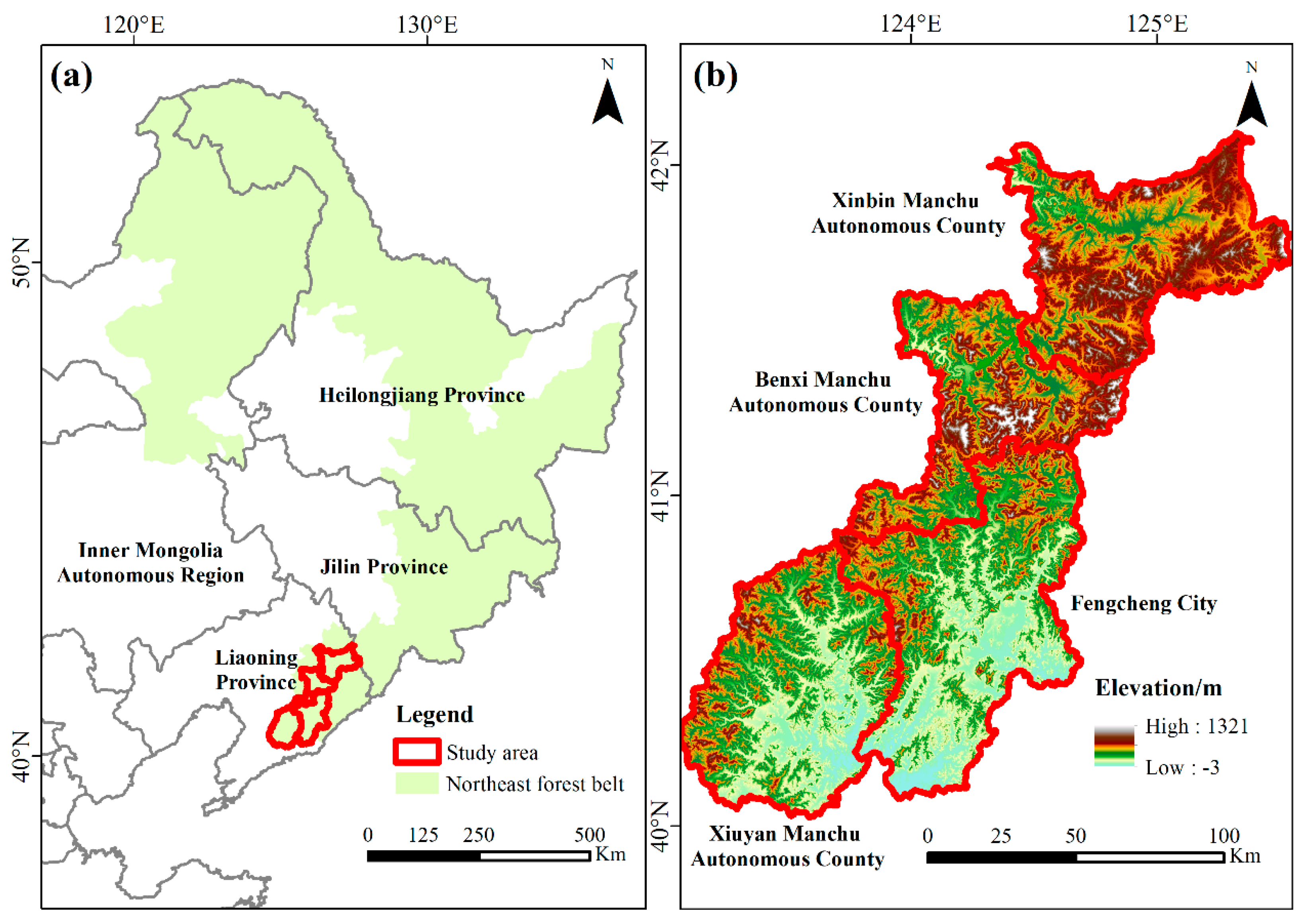
Located at the southern end of the belt in southeastern Liaoning, the Qianshan region includes Benxi, Xiuyan, Xinbin, and Fengcheng (Figure 1). It features a temperate humid monsoon climate, with annual precipitation of 400–900 mm and temperatures ranging from 5.2 °C to 11.7 °C. Despite its ecological value, Qianshan is a major mining area, with over 1000 active sites. Decades of intensive logging and mining have degraded forest quality and structure, weakening ecological functions. Assessing ecological vulnerability here is essential to support future conservation and restoration efforts.

2.2. Data Preparation

2.2.1. NDVI Dataset

The NDVI time series for the study area was constructed using the MOD13Q1 dataset. MODIS is a moderate−resolution imaging spectroradiometer carried by the Terra and Aqua satellites. It is a key instrument in the Earth Observing System (EOS) program for observing global biological and physical processes [44]. The MOD13Q1 product provides vegetation index data with a 16−day temporal resolution and a 250−m spatial resolution. Monthly NDVI time series data (2005–2024) were derived from MOD13Q1 16−day composites using the maximum value compositing method. The data were obtained from the USGS Land Processes Distributed Active Archive Center (LP DAAC) (https://lpdaac.usgs.gov/products/mod13q1v061/, accessed on 1 August 2026). Preprocessing of the data was performed using Google Earth Engine (GEE). Firstly, the MOD13Q1 dataset for the study area and desired timeframe was retrieved from the LP DAAC. Secondly, standard preprocessing steps such as mosaicking and clipping of the remote sensing images were performed. Finally, maximum value compositing was applied to NDVI data for the same month, resulting in the construction of an NDVI time series dataset for the study area spanning from 2005 to 2024.

2.2.2. Supporting Data

To examine the drivers of ecological resilience, this study selected indicators from two dimensions: natural factors and human activities (

Table 1. Data source and description of supporting data.

Data Description	Data Source
DEM	Hole−filled SRTM for the globe, Version 4, available from the CGIAR−CSI SRTM 90m Database (https://srtm.csi.cgiar.org, accessed on 1 August 2026)
Slope	calculated based on DEM data
Mining area	Natural Resources Department of Liaoning Province (https://zrzy.ln.gov.cn/, accessed on 1 August 2026)
Population	WorldPop Global Project Population Data (https://developers.google.com/earth-engine/datasets/catalog/WorldPop_GP_100m_pop, accessed on 1 August 2026)
Precipitation	National Earth System Science Data Center, National Science & Technology Infrastructure of China (https://www.geodata.cn/main/, accessed on 1 August 2026)
Temperature
Sunshine duration, Wind speed, Atmospheric pressure, and Humidity data	National Tibetan Plateau/Third Pole Environment Data Center (https://data.tpdc.ac.cn/, accessed on 1 August 2026)
Land Cover	Esri Land Cover (https://livingatlas.arcgis.com/landcover/, accessed on 1 August 2026)

). Climate, especially temperature and precipitation, plays a key role in vegetation dynamics and exhibits spatial heterogeneity across the Qianshan region due to varied conditions [45,46]. Additionally, the region’s mountainous terrain and intensive resource extraction highlight the need to assess interactions between climate, topography, and human disturbance [47].

Topographic variables (elevation and slope) were derived from the SRTM V4.1 DEM (90 m, resampled to 250 m). Mining site locations were obtained from Liaoning’s Department of Natural Resources, given the proven impact of mining on vegetation [48,49]. Mining density was used to reflect anthropogenic disturbance. Population data came from the WorldPop 100 m dataset, noted for its high resolution and accuracy [50].

Climate data (2005–2024) were sourced from the National Earth System Science Data Center, integrating CRU and WorldClim datasets and downscaled via the Delta method. The data were validated with 496 stations nationwide. Additional meteorological variables (sunshine, wind speed, pressure, humidity) were obtained from the National Tibetan Plateau Data Center. Monthly values were processed in R and averaged annually for analysis. Land use data were obtained from the Sentinel−2 10 m land cover dataset (Esri), providing detailed spatial input for evaluating ecological resilience.

2.3. Methodology

2.3.1. Breakpoint Detection

The BFAST algorithm (Breaks for Additive Seasonal and Trend algorithm) [51] was employed to identify breakpoints within the NDVI time series for the Qianshan region. The BFAST algorithm is a time series decomposition method that separates the original data into seasonal, trend, and remainder components. This enables effective detection of both seasonal and abrupt trend changes within the time series. The theoretical model is as follows:

$$Y_{{\mathrm{t}}^{\prime }}=T_{{\mathrm{t}}^{\prime }}+S_{{\mathrm{t}}^{\prime }}+e_{{\mathrm{t}}^{\prime }}(t^{\prime }=1,2,\dots ,n)$$

(1)

where $Y_{{\mathrm{t}}^{\prime }}$ represents the original data, $T_{{\mathrm{t}}^{\prime }}$ represents the trend component, $S_{{\mathrm{t}}^{\prime }}$ represents the seasonal component, $e_{{\mathrm{t}}^{\prime }}$ represents the residual component, t represents the observation time and n represents the length of the time series data.

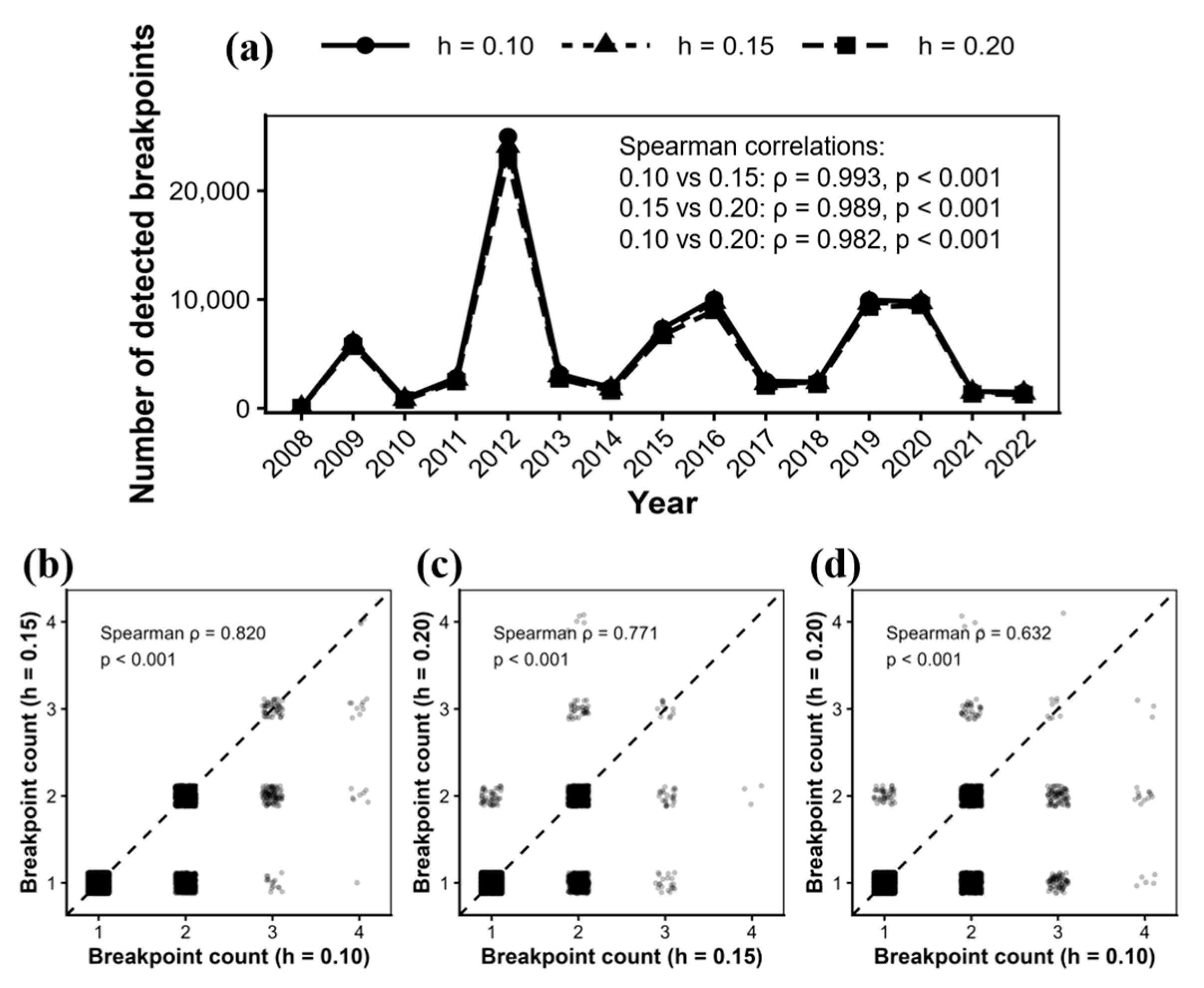
The BFAST algorithm uses Ordinary Least Squares residual−based Moving Sum (OLS−MOSUM) to determine whether breakpoints exist in the seasonal and trend components. The optimal number and timing of breakpoints are identified using the Bayesian Information Criterion (BIC). In this study, the BFAST algorithm was performed using the “bfast” package within R 4.5.0 programming environment (https://cran.r-project.org/web/packages/bfast/index.html, accessed on 10 August 2025). For parameter selection, previous research indicates that a higher number of iterations may lead to overfitting, whereas a lower number may fail to capture all breakpoints adequately. Therefore, the maximum number of iterations was set to 1, as a single iteration can substantially reduce computational costs while still enabling effective breakpoint detection [35]. To evaluate the robustness of breakpoint detection to the selection of h, sensitivity analyses were conducted using h values of 0.10, 0.15, and 0.20, while all other parameters and preprocessing procedures were kept unchanged. Temporal stability was assessed by comparing annual breakpoint counts from 2008 to 2022 and calculating pairwise Spearman rank correlations among the three annual breakpoint−count series (Figure 2a). Spatial stability was further evaluated by comparing the number of detected breakpoints per pixel under the three h settings and calculating pairwise pixel−level Spearman rank correlations (Figure 2b–d). The annual breakpoint−count series showed highly consistent temporal patterns, with pairwise Spearman correlation coefficients ranging from 0.982 to 0.993 (all p < 0.001). Pixel−level breakpoint counts were also significantly correlated, with coefficients ranging from 0.632 to 0.820 (all p < 0.001). Although smaller h values identified more pixels with multiple breakpoints and larger h values produced more conservative results, the principal temporal trends and relative spatial patterns remained stable. Therefore, h = 0.15 was selected for the main analysis because it provided an appropriate balance between breakpoint−detection sensitivity and result stability.

All other parameters were kept at their default values [52]. The detailed parameter settings are summarized in

Table 2. Parameter of BFAST algorithm.

Parameter	Description	Value
Yt	Time series to be analyzed	NDVI Time series
h	minimal segment size between potentially detected breaks in the trend model given as fraction relative to the sample size	0.15
max.iter	maximum amount of iterations allowed for estimation of breakpoints in seasonal and trend component.	1
breaks	integer specifying the maximal number of breaks to be calculated	default
decomp	the function to use for decomposition. stl can handle sparse time series	stlplus
level	threshold value for structured test	0.05
season	the seasonal model used to fit the seasonal component and detect seasonal breaks	harmonic

:

Before breakpoint detection, quality−control procedures were applied to reduce pseudo−breakpoints associated with meteorological noise and poor−quality observations. Observations affected by clouds, cloud shadows, snow cover, or other low−quality conditions were removed according to the quality−control information provided with the MODIS NDVI product. Missing observations generated by this screening were reconstructed using temporal interpolation to maintain the continuity of the NDVI time series and to prevent isolated abnormal observations from being interpreted as structural changes. In addition, anomalous years were identified by jointly examining regional meteorological records and the temporal consistency of NDVI variations across the study area. Years characterized by widespread and synchronous NDVI anomalies that coincided with documented regional meteorological extremes, such as abnormal precipitation, persistent snow cover, or unusually low temperatures, were regarded as meteorologically anomalous years and excluded before BFAST analysis. This procedure was intended to distinguish short−term regional climate anomalies from persistent vegetation structural changes. No additional breakpoint−magnitude threshold was imposed, and all breakpoints detected from the quality−controlled NDVI time series were retained for subsequent analysis.

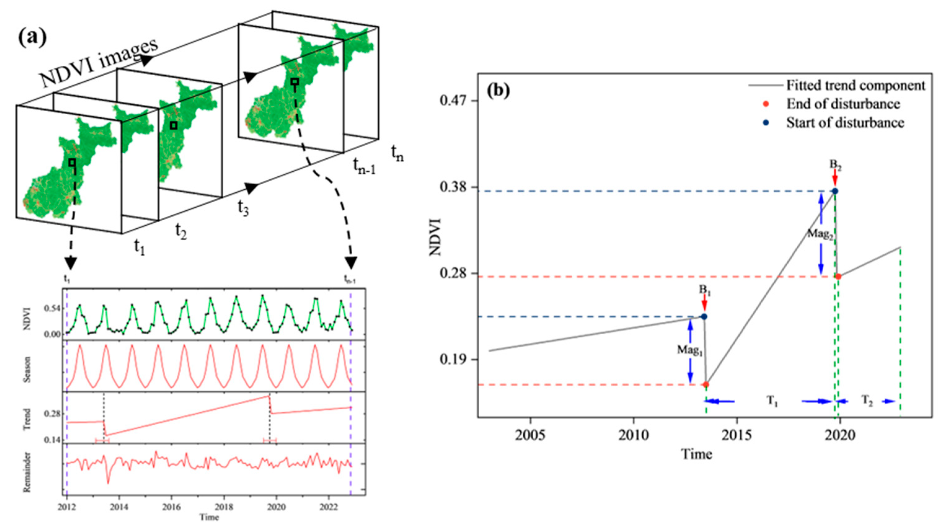
The results of the BFAST algorithm are shown in the figure below. The “NDVI” in Figure 3a represents the original pixel NDVI time series. The “Season” corresponds to the seasonal component; the “Trend” corresponds to the trend component, which contains 2 trend breakpoints marked by vertical dashed black lines. The confidence intervals for the estimated change times are also shown. The “Remainder” corresponds to the remainder component. B₁ and B₂ represent the trend breakpoints, while Mag₁ and Mag₂ are the corresponding magnitudes. The magnitude reflects the magnitude of change in vegetation status between the end of a disturbance and its beginning. A larger magnitude indicates a more significant disturbance to the vegetation. T₁ and T₂ represent the recovery times associated with each trend change. They indicate the duration it took for vegetation to recover after the respective disturbances.

2.3.2. Quantification of Recovery and Resistance

In this study, only vegetated pixels were considered for the quantification of ecological recovery and resistance. Ecological resistance reflects the ability of vegetation to maintain a stable state when subjected to external disturbances, while disturbance magnitude indicates the intensity of the disturbance. Higher resistance implies that vegetation exhibits a smaller response to a given disturbance, indicating greater ecosystem stability; conversely, lower resistance corresponds to stronger vegetation responses and reduced ecosystem stability. The specific calculation formula is provided in Equation (2).

$$Resistanc{e}_i={\displaystyle \frac{1}{n_i}}{\displaystyle \sum _{j=1}^{n_i}\frac{Ma{g}_{\max }-Ma{g}_{ij}}{Ma{g}_{\max }-Ma{g}_{\min }}}$$

(2)

where $Resistanc{e}_{\mathrm{i}}$ represents the ecological resistance of pixel i across all detected disturbance events, $n_i$ is the total number of breakpoints detected for pixel i. $Ma{g}_{i,j}$ denotes the magnitude of the j−th breakpoint detected in pixel i. $Ma{g}_{\max }$ and $Ma{g}_{\min }$ represent the maximum and minimum breakpoint magnitudes among all detected disturbance events in the study area, respectively.

Recovery capability was assessed for vegetated pixels (forest and grassland) following the first identified breakpoint (B₁) in the NDVI time series. This reflects the vegetation’s response to the initial disturbance event. The specific formulas used are presented in Equations (3)–(6). The slope $k$ of the post−breakpoint trend term in the NDVI time series was calculated. A positive value of $k$ ($k\ge 0$) indicates a recovery trend in vegetation after the disturbance. In this case, the definite integral of NDVI for each year ($j$) of the recovery period for pixel $i$, denoted as $NDV{I}_{\text{recovery},i,j}$, was calculated using Equation (3).

$${\mathit{\text{NDVI}}}_{\text{recover},i,j}={\displaystyle {\int }_{t_{1,j}}^{t_{2,j}}f(t,i,j)}d(t)$$

(3)

where $f(t,i,j)$ represents the fitted curve of the NDVI time series for pixel $i$ in year $j$, and ${\mathrm{t}}_{1,j}{,\mathrm{t}}_{2,j}$ denote the starting and ending months of the integration period in year $j$, respectively. $NDV{I}_{\text{recovery},i,j}$ represents the annual integrated NDVI and reflects the cumulative vegetation growth status of pixel i during that year.

Secondly, the difference in NDVI growth $\mathrm{\Delta }NDV{I}_{\text{recovery},i,j}$ between subsequent years ($j$ and $j+1$) was calculated using Equation (4). This represents the annual recovery rate for pixel $i$. The total vegetation recovery (TVR) for the pixel was then obtained by summing the annual recovery rates across the entire recovery period.

$$TV{R}_{\mathrm{i}}={\displaystyle \sum _{\mathrm{j}=1}^{\mathrm{n}}(NDV{I}_{\mathrm{recovery},\mathrm{i},\mathrm{j}+1}}-NDV{I}_{\mathrm{recovery},\mathrm{i},\mathrm{j}})$$

(4)

Subsequently, the average recovery value for each pixel was calculated using Equation (5) to obtain a single metric representing overall recovery capability.

$$Recover{y}_{\mathrm{i}}^{\mathrm{raw}}=TV{R}_{\mathrm{i}}/\mathrm{n}$$

(5)

Finally, recovery was normalized using Equation (6) to obtain the recovery value.

$$Recover{y}_i={\displaystyle \frac{Recover{y}_i^{raw}-Recover{y}_{\min }^{raw}}{Recover{y}_{\max }^{raw}-Recover{y}_{\min }^{raw}}}$$

(6)

where $Recover{y}_i$ represents the normalized ecological recovery capacity of pixel i, $Recover{y}_i^{raw}$ is its mean annual recovery value. $Recover{y}_{\min }^{raw}$ and $Recover{y}_{\max }^{raw}$ are the maximum and minimum raw recovery values among all evaluated pixels, respectively. A value closer to 1 indicates stronger recovery capacity, whereas a value closer to 0 indicates weaker recovery capacity.

2.3.3. Analysis of Ecological Resistance and Recovery Driving Factors

The Optimal Parameters−Based Geographical Detector (OPGD) is a statistical analysis tool engineered to identify spatial heterogeneity and its underlying driving mechanisms [53]. This method is particularly adept at determining spatial consistency between explanatory and dependent variables, effectively revealing if a spatial coupling relationship exists. Unlike traditional methods, the geographical detector doesn’t require assumptions of linear relationships between variables. It excels at handling nonlinearities, non−normal distributions, and other complex data structures. Consequently, the OPGD has seen extensive application in studies identifying spatial driving factors across diverse fields, including ecological environments, land use, and public health [54,55,56,57].

Meteorological and topographic conditions are crucial natural factors that significantly influence vegetation growth and ecosystem dynamics. Therefore, elevation, topographic variation (slope), and precipitation were selected as meteorological and topographic input variables to characterize the influence of natural environmental conditions on vegetation recovery and resistance. Simultaneously, recognizing the Qianshan region’s abundant mineral resources and intensive mining activities, which have caused evident disturbances to local ecosystems, mining density was introduced as a key indicator of human activity intensity to assess its potential impact on ecosystem stability. Considering both natural factors and human−induced disturbances, a total of nine driving factors were selected for OPGD analysis to explore their driving effects on the spatial distribution of vegetation ecological recovery and resistance. Details of the variables and their data sources are provided in

Table 3. The index of natural factors in the study area.

Index	Abbreviation	Unit
Annual precipitation	PRE	mm
Average annual temperature	TEM	°C
Annual sunshine duration	SSD	h
Average annual wind speed	WIN	m/s
Density of mining area	DEN	points/km2
Elevation	ELE	m
Slope	SLO	°
Average air pressure	PRS	hPa
Population density	POP	People/km2
Average annual relative humidity	RHU	%
Landuse	LAN	/

.

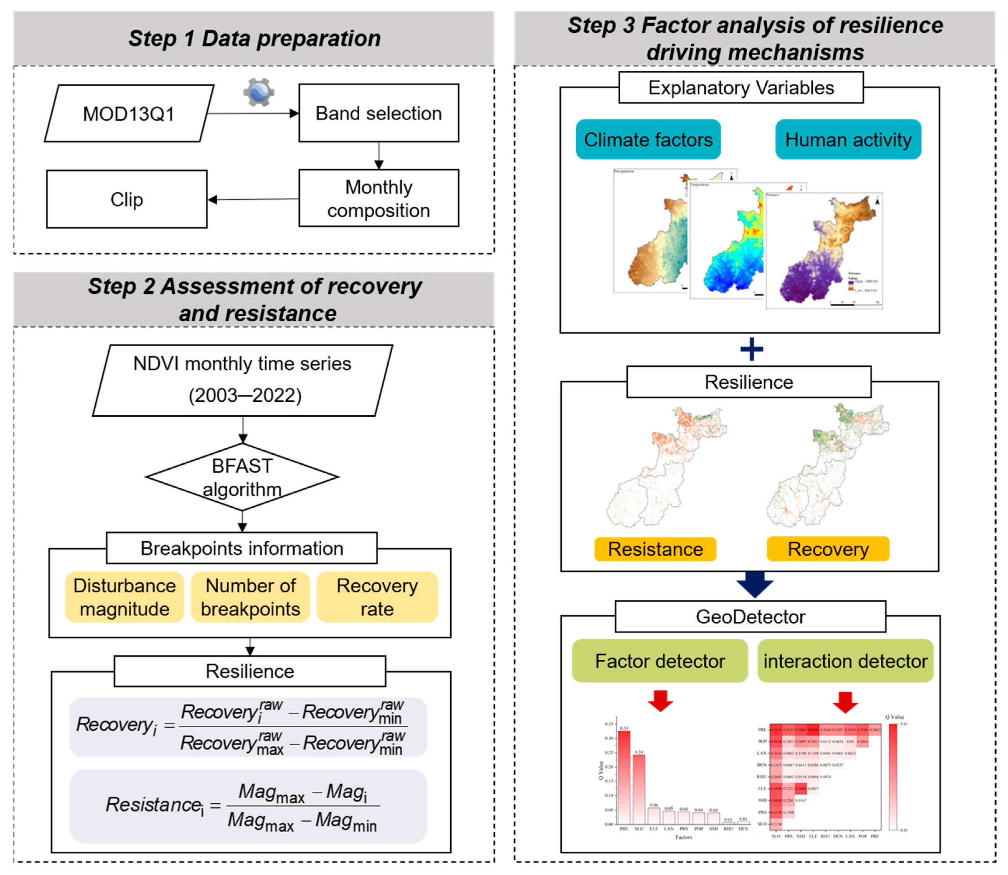
Strong correlations among explanatory variables may lead to biased analysis results, ultimately reducing both the explanatory power and stability of the model. Therefore, this study employed the Variance Inflation Factor (VIF) to test for multicollinearity among variables and to guide the selection of explanatory factors accordingly. The VIF value reflects the degree of linear correlation between a variable and all other explanatory variables; higher VIF values indicate more severe multicollinearity. It is generally accepted that when the VIF value of a variable exceeds 7.5, it indicates strong multicollinearity with other variables, and such a variable should be removed or adjusted [58,59]. The specific procedure is as follows: first, VIF values were calculated for all candidate factors. The variable with the highest VIF was identified and removed. The VIF values were then recalculated for the remaining variables, and this process was repeated until all retained variables had VIF values below 7.5, resulting in a multicollinearity−free set of variables for OPGD analysis. After determining the final set of analysis factors, the optimal discretization method and number of categories were calculated for each variable to enhance the explanatory power of the Geographical Detector model. Subsequently, invalid values were removed to ensure the quality and completeness of the input data. Finally, the processed data were input into the Geographical Detector tool to explore the spatial distribution patterns of ecological recovery and resistance at the pixel scale, as well as their relationships with natural and anthropogenic driving factors. The workflow of this study is showed in Figure 4.

3. Results

3.1. Spatiotemporal Characteristics of Vegetation Disturbances

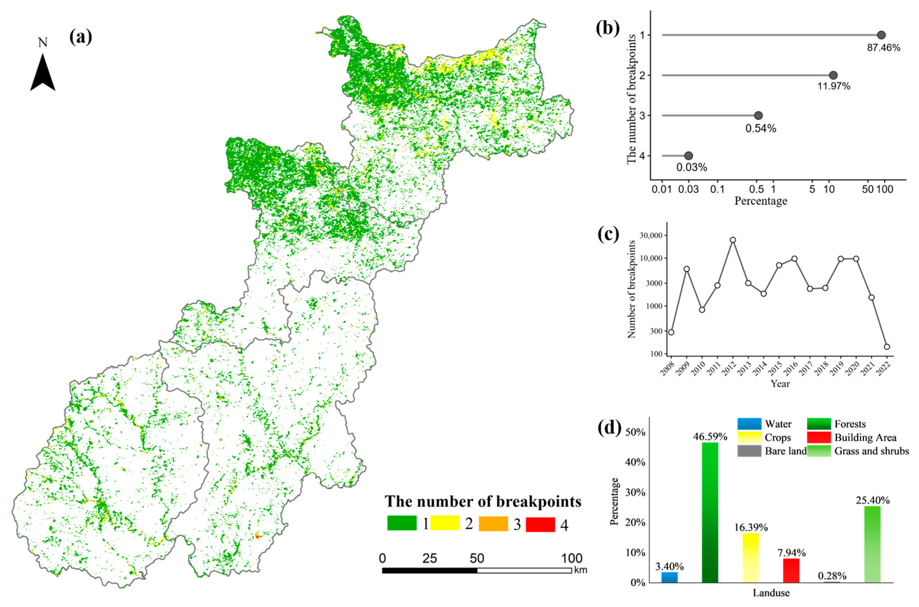
Figure 5 illustrates the spatial, frequency, temporal, and land cover distribution characteristics of NDVI breakpoint pixels. First, regarding spatial distribution (Figure 5a), breakpoint pixels are widely distributed across the study area. There’s a notable concentration in the northern forested region, which indicates this area experienced more significant vegetation disturbances during the study period.

From 2005 to 2024, pixels within the study area experienced between one and five NDVI breakpoints (Figure 5b). The vast majority of pixels—as much as 87.46%—exhibited only one breakpoint. Pixels with two breakpoints made up 11.97%, while those with three and four breakpoints were relatively rare, accounting for 0.54% and 0.03%, respectively.

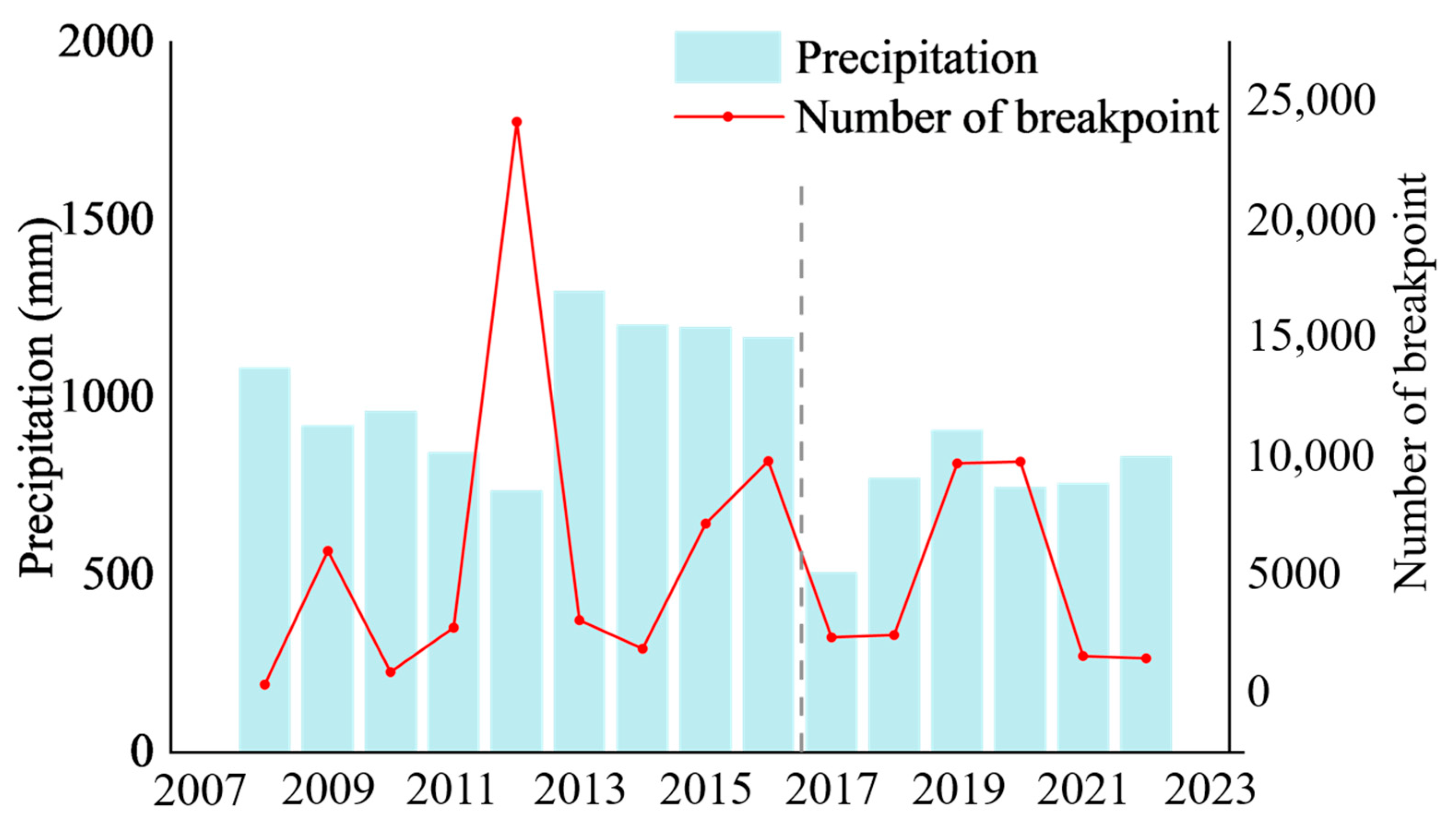
Figure 5c illustrates the temporal distribution of breakpoint events. The year 2012 recorded the highest concentration of breakpoints, with 24,118 events. This was followed by 2016, 2020, and 2019, each experiencing over 9000 breakpoints. Overall, the number of breakpoints showed a marked increasing trend during the periods of 2008–2012, 2014–2016, and 2018–2020, indicating more frequent vegetation disturbance events in those years. Regarding land cover types (Figure 5d), breakpoint pixels were predominantly concentrated in forested areas, accounting for 46.59%. Grasslands and croplands followed, making up 25.40% and 16.39%, respectively.

3.2. Assessment of Recovery and Resistance

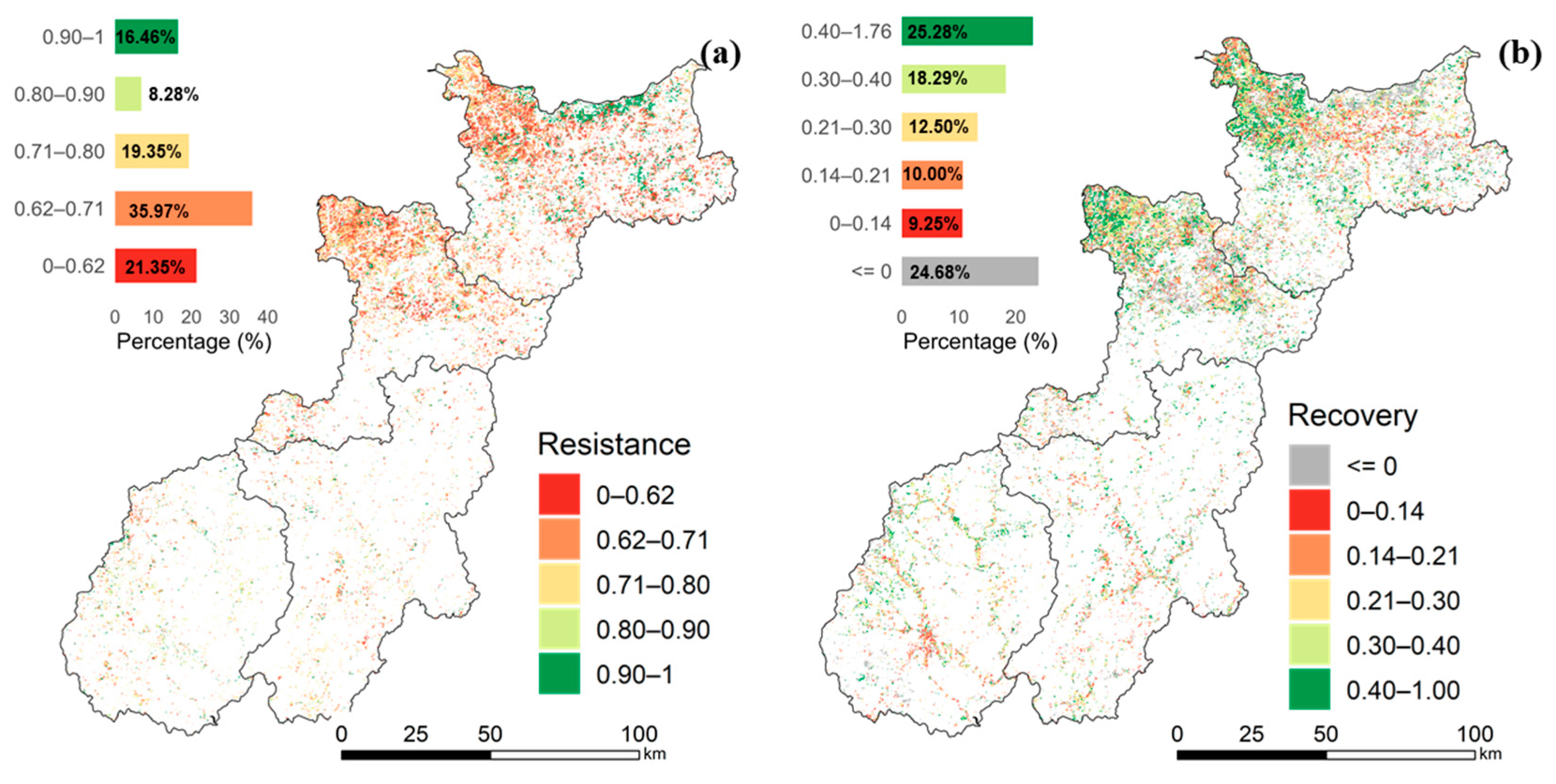
Figure 6a illustrates the spatial distribution of ecological resistance throughout the Qianshan region. Our analysis shows that 35.97% of the area has an ecological resistance between 0.62 and 0.71, which is the highest proportion observed. In contrast, only 8.28% of the region falls within the lowest ecological resistance range, specifically 0.80 to 0.90.

Figure 6b shows the spatial distribution of vegetation recovery in the Qianshan region. This analysis focuses specifically on pixels impacted by external disturbances, as indicated by NDVI changes. Approximately 24.68% of these disturbed pixels exhibited no recovery, signifying a continuous decline in vegetation health after the disturbance. For pixels that did recover, the highest proportion, 25.28%, showed recovery values ranging from 0.40 to 1.00. Recovery values then progressively decreased in the subsequent categories: 0.30–0.40 (18.29%), 0.21–0.30 (12.50%), and 0.14–0.21 (10.0%). Only 9.25% of pixels displayed minimal recovery, falling within the 0–0.14 range.

Ecological resistance and recovery differed markedly among land−cover types (

Table 4. Mean ecological resistance and recovery across different land−cover types.

Land−Cover Type	Mean Resistance	Mean Recovery
Forest	0.641	0.435
Shrubland	0.576	0.514
Grassland	0.497	0.662
Cropland	0.424	0.595

). Forests exhibited the highest mean resistance (0.641), followed by shrublands (0.576) and grasslands (0.497), whereas croplands had the lowest mean resistance (0.424). In contrast, grasslands showed the highest mean recovery (0.662), followed by croplands (0.595), while shrublands and forests had mean recovery values of 0.514 and 0.435, respectively. Overall, woody vegetation types, including forests and shrublands, exhibited relatively high resistance but comparatively low recovery capacity, whereas grasslands and croplands showed lower resistance but greater post−disturbance recovery capacity. These differences may be related to the deeper root systems, more stable community structures, and slower regeneration processes of woody vegetation, whereas the shorter life cycles and faster regeneration rates of herbaceous vegetation may facilitate more rapid recovery following disturbance. The relatively high recovery capacity of croplands may also be influenced by human management practices, including cultivation, irrigation, and vegetation re−establishment [60].

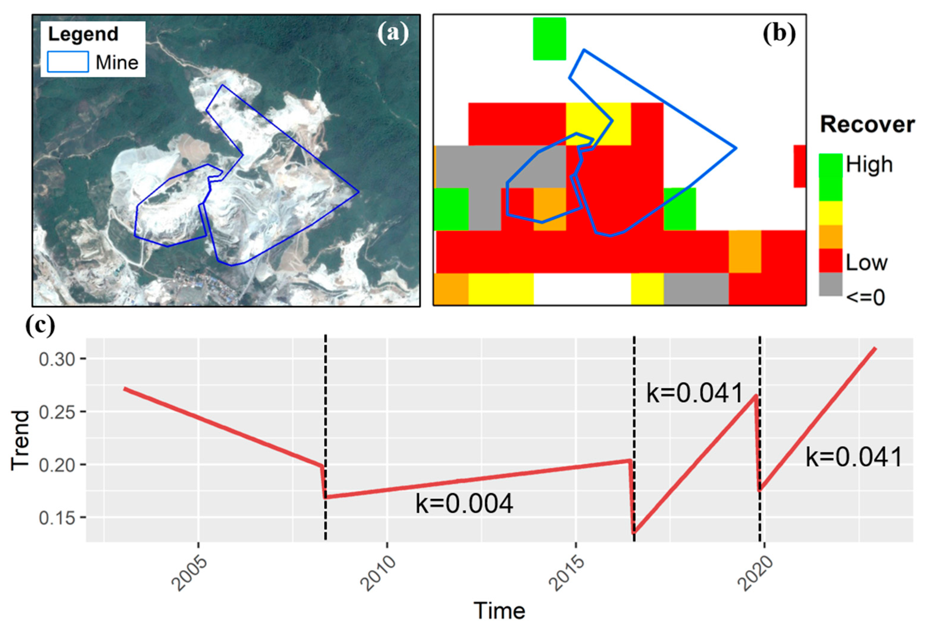
Figure 7 provides an example illustrating the difference between the proposed recovery indicator and a conventional trend−based assessment in an open−pit mining area. Although the segmented NDVI trend showed positive slopes during several periods, the corresponding area remained largely characterized by bare or sparsely vegetated surfaces. The spatial recovery assessment identified extensive pixels with low or non−positive recovery values within and around the mining boundary. This example indicates that a positive long−term or segmental NDVI trend does not necessarily correspond to effective vegetation recovery, particularly in strongly disturbed landscapes.

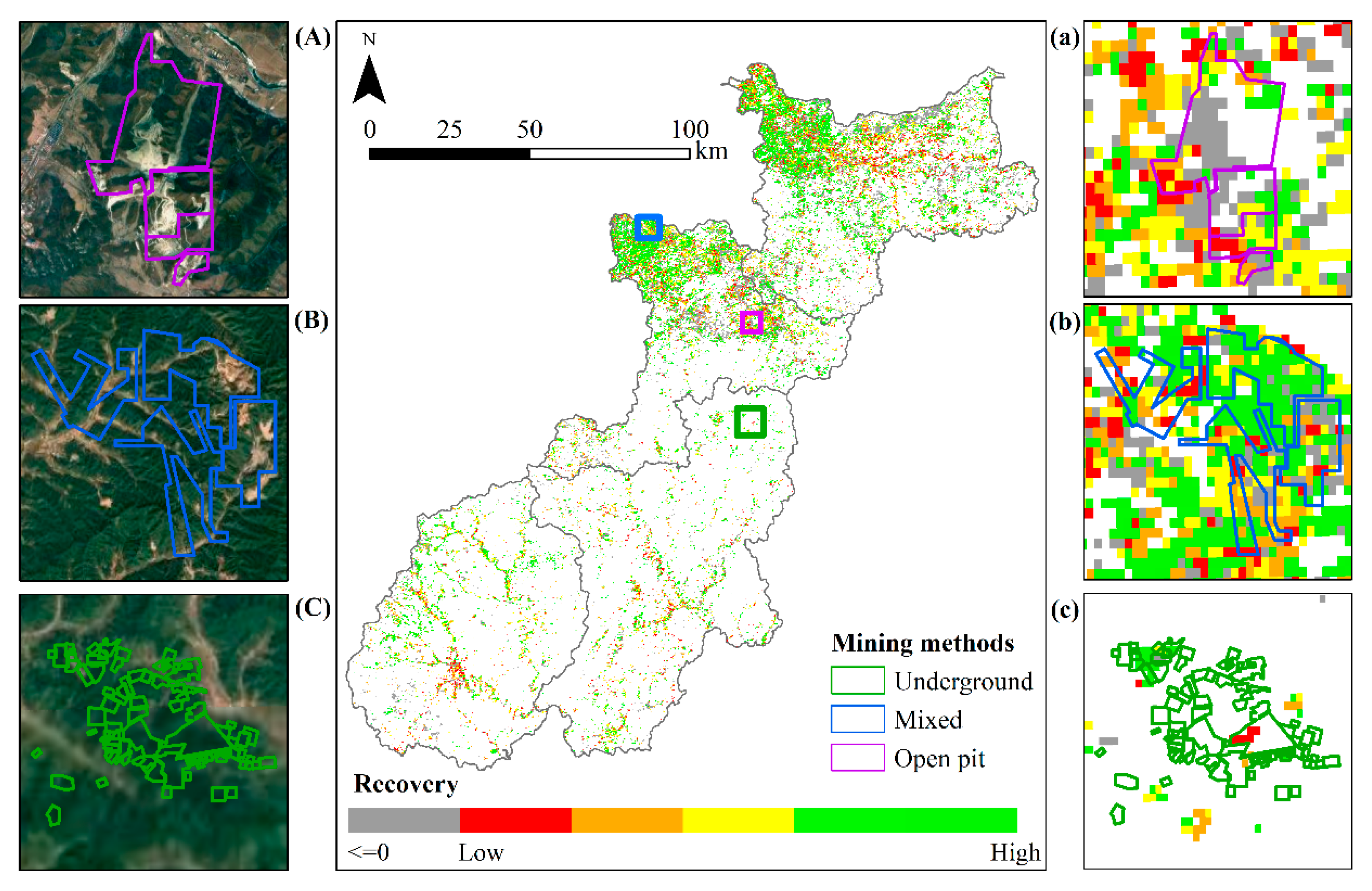
Figure 8 further shows the spatial variation in vegetation recovery among different mining types. Recovery conditions were generally poorer within mining−affected areas than in their surrounding landscapes, but clear differences were observed among mining types. Open−pit mining areas were dominated by low or non−positive recovery values, whereas mixed and underground mining areas showed more heterogeneous recovery patterns. Some underground mining areas also contained localized pixels with low recovery despite relatively limited visible surface disturbance. These spatial differences demonstrate that vegetation recovery varies substantially among mining types and within individual mining−affected areas.

3.3. Contribution of Natural Factors to Recovery and Resistance

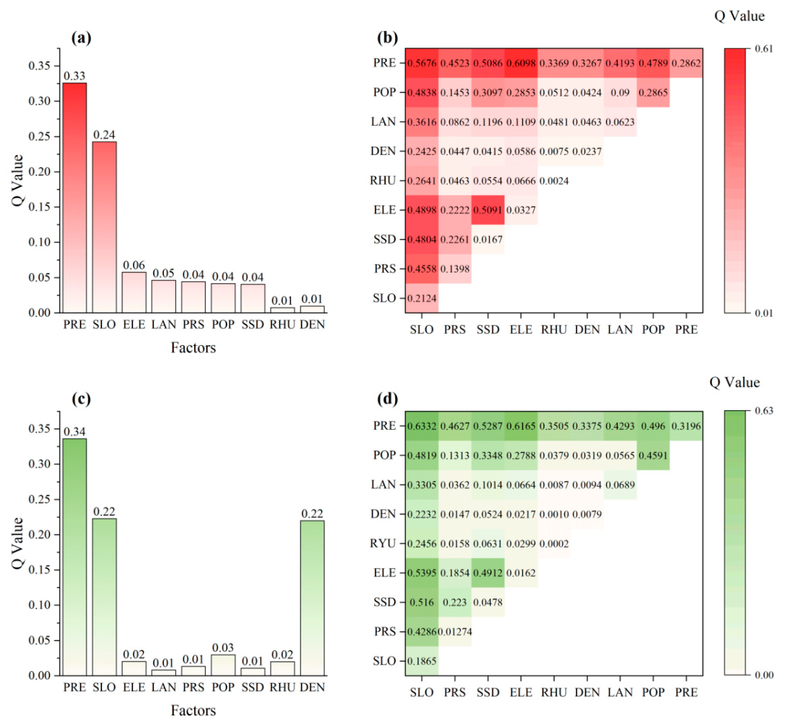
After conducting the VIF analysis to address multicollinearity, two factors were excluded: annual average temperature and annual average wind speed. The final selection of factors for calculation includes PRE, SLO, ELE, LAN, PRS, POP, SSD, RHU, and DEN.

To assess the sensitivity of the OPGD results to the number of discretization classes, the q−values of all explanatory factors were recalculated using 4, 5, 6, 7, and 8 classes while keeping the discretization method and all other analytical settings unchanged. The results showed that changes in the number of classes caused only minor variations in the individual q−values, whereas the rankings of the key factors remained generally stable (

Table 5. Sensitivity of factor q−values for ecological resistance to the number of discretization classes.

Factor	4 Classes	5 Classes	6 Classes	7 Classes	8 Classes
PRE	0.312	0.324	0.330	0.336	0.331
SLO	0.226	0.235	0.240	0.244	0.239
ELE	0.055	0.059	0.060	0.062	0.061
LAN	0.046	0.049	0.050	0.051	0.050
PRS	0.039	0.041	0.040	0.043	0.042
POP	0.036	0.038	0.040	0.041	0.040
SSD	0.034	0.037	0.040	0.039	0.038
RHU	0.012	0.011	0.010	0.011	0.012
DEN	0.010	0.010	0.010	0.01	0.011
Spearman’s $\mathsf{\rho }$ with the 6−class scheme	0.979	0.979	1.000	0.979	0.979

and

Table 6. Sensitivity of factor $\mathrm{q}$−values for ecological recovery to the number of discretization classes.

Factor	4 Classes	5 Classes	6 Classes	7 Classes	8 Classes
PRE	0.321	0.333	0.340	0.346	0.341
SLO	0.207	0.216	0.220	0.224	0.221
ELE	0.019	0.020	0.020	0.021	0.020
LAN	0.012	0.011	0.010	0.011	0.012
PRS	0.011	0.010	0.010	0.010	0.011
POP	0.027	0.029	0.030	0.031	0.030
SSD	0.012	0.011	0.010	0.011	0.010
RHU	0.018	0.019	0.020	0.021	0.020
DEN	0.205	0.214	0.220	0.222	0.219
$\mathrm{Spearman}\text{’}\mathrm{s}\mathsf{\rho }$ with the 6−class scheme	0.979	0.979	1.000	0.983	0.979

). For ecological resistance, precipitation consistently exhibited the highest spatial explanatory power across all classification schemes, with q−values ranging from 0.312 to 0.336, while slope consistently ranked second, with q−values ranging from 0.226 to 0.244. For ecological recovery, precipitation retained the highest explanatory power under all classification schemes, with q−values ranging from 0.321 to 0.346, whereas slope and mining−area density consistently ranked second and third, with q−values ranging from 0.207 to 0.224 and from 0.205 to 0.222, respectively. Using the six−class scheme as the reference, the Spearman rank correlation coefficients for factor rankings under the alternative classification schemes were all no lower than 0.979, indicating that the identification and relative ranking of the key factors were highly stable across different numbers of discretization classes.

The results of the OPGD model analysis are presented in Figure 9. The Q−value indicates an independent variable’s explanatory power over a dependent variable, with a higher Q−value signifying a stronger influence on the dependent variable’s spatial distribution. Figure 9a and Figure 9c display the single−factor analysis results for ecological resistance and recovery, respectively. Precipitation and slope were identified as the primary factors impacting both resistance and recovery throughout the Qianshan region. Furthermore, mining area density significantly influenced recovery, suggesting a potential negative effect of mining activities on vegetation resilience.

Figure 9b,d show the explanatory power of factor interactions for the spatial differentiation of ecological resistance and recovery. The results indicate that the q−values of most two−factor interactions were higher than those of the corresponding individual factors, suggesting that the spatial differentiation of resistance and recovery was better explained by interacting factors than by single factors alone. Interactions involving precipitation or slope generally exhibited relatively high explanatory power. Specifically, the interaction between precipitation and elevation showed nonlinear enhancement and had the strongest explanatory power for the spatial differentiation of resistance (q = 0.6098). In contrast, the interaction between precipitation and slope showed bilinear enhancement and had the strongest explanatory power for the spatial differentiation of recovery (q = 0.6332). These results indicate that the interactions of precipitation with elevation and slope are important for explaining the spatial differentiation of ecological resistance and recovery across the Qianshan region.

The temporal relationship between annual precipitation and breakpoint occurrence is shown in Figure 10. From 2007 to 2009, annual precipitation decreased while the number of breakpoints increased, reaching a peak in 2009. In 2010, precipitation increased markedly and breakpoint numbers declined. From 2010 to 2013, precipitation decreased again, accompanied by a general increase in breakpoint occurrence. After 2016, however, the correspondence between annual precipitation and breakpoint numbers became weaker. Spatially, precipitation generally decreased from northwest to southeast, whereas breakpoint density showed an approximately opposite pattern.

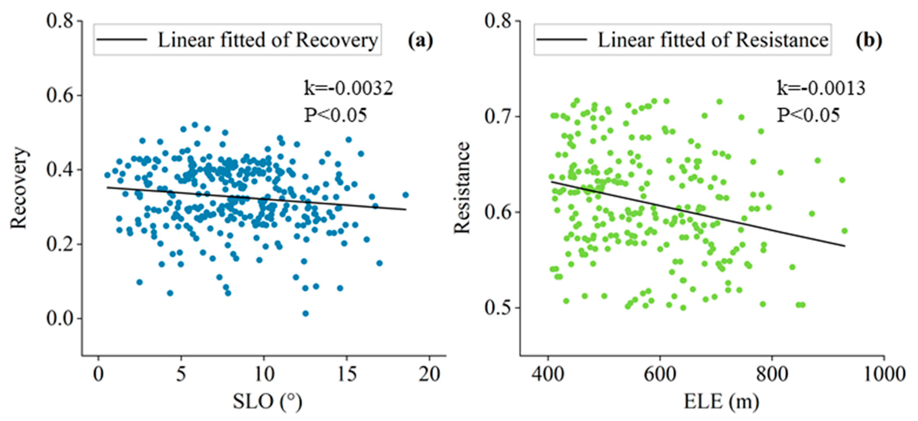
To supplement the OPGD results with information on the direction of statistical associations, precipitation, elevation, and slope were further examined using multiple linear regression (

Table 7. The coefficients of the regression equations.

Regression Coefficients		Independent Variable
		ELE	SLO	PRE
dependent variable	resistance	−0.190	/	0.058
	recovery	/	−0.123	0.024

). Precipitation was positively associated with both ecological resistance and recovery, whereas slope and elevation generally showed negative associations. These results were consistent with the spatial patterns of ecological resilience, particularly in the northern mountainous areas characterized by relatively steep terrain (Figure 11). Mining−related differences in vegetation recovery were also evident in Figure 9. Open−pit mining areas showed the lowest mean recovery value (0.13), and approximately 30% of pixels had recovery values of ≤0. Mixed mining and underground mining areas exhibited slightly higher mean recovery values of 0.20 and 0.23, respectively, but these values remained lower than those observed in non−mining areas. Some underground mining areas also showed very low vegetation recovery values, indicating considerable spatial heterogeneity in recovery among mining−affected areas.

4. Discussion

4.1. Effectiveness of the Proposed Indicators for Vegetation Recovery and Resistance

The contrast between the trend−based assessment and the recovery indicator highlights an important methodological issue in evaluating post−disturbance vegetation dynamics. A positive NDVI slope may reflect a gradual increase from a very low vegetation baseline, short−term greening, or fluctuations associated with mixed land−cover components [61,62], rather than a genuine return toward a stable vegetated state. This limitation becomes particularly relevant in severely disturbed environments such as open−pit mines, where exposed soil, fragmented vegetation, and heterogeneous surface conditions can produce apparent positive trends without substantial ecological recovery. By considering changes in the accumulated NDVI trajectory during the post−disturbance period, the proposed indicator is less dependent on a single fitted trend and is therefore better able to distinguish sustained recovery from temporary or incomplete greening. This distinction is important because overestimating recovery in heavily disturbed areas may lead to an overly optimistic assessment of restoration effectiveness.

4.2. Uncovering Spatial Drivers of Ecological Resilience

The OPGD analysis showed that precipitation was one of the most important fac−tors associated with the spatial differentiation of ecological recovery and resistance. This finding is consistent with previous studies showing that water availability plays a key role in regulating vegetation stability and post−disturbance recovery [14,63]. Reduced precipitation can intensify vegetation water stress and increase susceptibility to disturbance, whereas wetter conditions can improve soil moisture availability and support vegetation recovery. The temporal relationship between precipitation and breakpoint occurrence further suggests that vegetation responses to precipitation variability may involve a time lag, as soil moisture depletion, cumulative physiological stress, and canopy decline often develop gradually rather than instantaneously [14]. The weakening relationship between precipitation and breakpoint occurrence after 2016 suggests that vegetation dynamics may have increasingly reflected the combined influence of climate, vegetation development, ecological restoration, and human disturbance [64,65]. As restored vegetation matured, deeper root systems, greater canopy cover, and improved microclimatic regulation may have enhanced resistance to short−term precipitation fluctuations [66]. Long−term restoration may also have improved soil retention and local water regulation, thereby reducing vegetation sensitivity to annual precipitation variability [67,68]. At the same time, mining, land−use change, forest management, and other anthropogenic disturbances may have generated vegetation changes that were not synchronized with precipitation, further weakening the apparent climate–disturbance relationship.

Topographic factors also contributed to the spatial differentiation of ecological resilience. The negative associations of slope and elevation with recovery and resistance may reflect differences in water retention, soil erosion, root development, temperature, and growing−season conditions. Steeper terrain can reduce soil stability and water availability, while higher elevations may impose additional climatic constraints on vegetation growth. These effects help explain why ecological recovery capacity varies substantially across the mountainous parts of the study area.

Although mining density had relatively limited explanatory power at the regional scale, mining disturbance can still produce strong localized ecological effects. The spatial differences among mining types further suggest that the effects of mining on vegetation recovery depend strongly on disturbance mechanisms rather than on mining presence alone. Open−pit mining causes direct vegetation removal and severe surface disturbance, whereas underground mining may generate slower and less visible impacts through changes in soil structure, moisture conditions, and subsurface processes [69]. Mixed mining areas may combine these disturbance pathways and therefore exhibit more complex recovery patterns. These differences also help explain why a simple mining−density indicator may have limited explanatory power at the regional scale, because it cannot fully represent variations in mining method, disturbance intensity, operational stage, or reclamation history. The relatively weak regional contribution of mining density should therefore not be interpreted as evidence of negligible ecological impact. Instead, it indicates that mining effects are spatially concentrated and may be partly masked when evaluated across a large and environmentally heterogeneous region.

Overall, ecological resistance and recovery in the Qianshan region reflect the combined influence of climatic conditions, topography, vegetation development, restoration history, and human disturbance. These interacting controls highlight the need to interpret ecological resilience within a multi−factor framework rather than attributing spatial patterns to any single driver. Future studies should incorporate longer−term ecological monitoring, more detailed disturbance histories, and temporally explicit mining and restoration data to better identify the mechanisms underlying changes in vegetation resilience.

4.3. Limitations and Future Research

While this study advances the understanding of ecological resistance and recovery, several limitations remain. First, the MOD13Q1 dataset, though valuable, has a coarse resolution that may overlook fine−scale vegetation changes. Future work could integrate higher−resolution imagery for improved accuracy. Second, the analysis emphasized precipitation, slope, and elevation, but other factors like soil type and dominant vegetation may also influence ecological responses. Including these variables could yield a more nuanced understanding. Additionally, although time−series algorithms effectively detected NDVI breakpoints, exploring alternatives such as LandTrendr may enhance result robustness. Comparative analyses could help identify the most suitable methods for specific contexts. Lastly, the current approach shows limited sensitivity to impacts from underground mining. Incorporating indicators like soil moisture may better capture such disturbances. Addressing these limitations can improve future assessments of ecological resilience in complex landscapes.

Another limitation is that the effects of mining activities were not quantitatively differentiated according to mining characteristics or disturbance intensity. The available mining dataset primarily represents the spatial distribution of mining areas and does not provide temporally consistent information on mining−area extent, extraction intensity, mining method, operational stage, or reclamation timing. Consequently, mining−related disturbance was represented using a relatively simplified spatial indicator, which may obscure differences in ecological responses among active mines, abandoned mines, and reclaimed mining areas. Mining operations of different scales and intensities may produce substantially different effects on soil conditions, hydrological processes, vegetation structure, and subsequent ecological recovery. Future research should integrate multi−temporal mining boundaries, production records, extraction intensity, mining methods, and reclamation histories to develop more detailed indicators of mining disturbance. Such information would allow ecological resistance and recovery to be compared quantitatively across different mining intensities, operational stages, and restoration conditions. A further limitation is that resistance was quantified only for pixels with detected negative breakpoints. Pixels without detected breakpoints were not assigned resistance values because the absence of a breakpoint may indicate either high resistance to disturbance or simply a lack of disturbance during the study period. Therefore, the resulting resistance map represents resistance conditional on detected disturbance and should not be interpreted as a complete assessment of resistance across all vegetation pixels. Future studies should integrate independent disturbance records or exposure indicators to distinguish undisturbed areas from highly resistant areas.

Detailed information on dominant tree species and stand−age structure was unavailable across the entire study area. Because these stand characteristics may influence vegetation resistance and recovery, future studies should integrate forest inventory data to examine ecological resilience across different species compositions and stand−age classes.

5. Conclusions

This study employed the BFAST detection algorithm to analyze long−term Normalized Difference Vegetation Index (NDVI) time series in the Qianshan region of the northeastern forest belt and to quantify ecological resistance and recovery using breakpoint count, magnitude, and average NDVI growth rate. The main findings are as follows: (1) Vegetation disturbances were predominantly episodic, with most pixels experiencing only one detected breakpoint during the study period. (2) Vegetation generally showed relatively low resistance but comparatively strong recovery, with more than 70% of disturbed pixels exhibiting subsequent recovery. Resistance and recovery differed among land−cover types. Forests had the highest mean resistance (0.641), whereas grasslands showed the highest mean recovery (0.662). Overall, woody vegetation was more resistant but recovered more slowly, while grasslands and croplands exhibited lower resistance but stronger post−disturbance recovery. (3) The spatial patterns of resistance and recovery were jointly influenced by natural and anthropogenic factors. Precipitation and slope showed relatively high explanatory power, while interactions among environmental factors further strengthened their effects. Mining activities had limited regional explanatory power but caused clear localized constraints on vegetation recovery, particularly in open−pit mining areas.

This study contributes to the advancement of ecological resistance and recovery assessment methodologies. The findings provide valuable information for guiding ecological restoration efforts and environmental management practices within the Qianshan region of the northeastern forest belt. By elucidating the influence of both natural (precipitation, elevation, slope) and anthropogenic (mining activities) factors on ecological resilience, this research offers critical insights that can inform strategies to enhance regional recovery potential and resistance to future disturbances.

References

1. Lin, J.-C.; Chiou, C.-R.; Chan, W.-H.; Wu, M.-S. Valuation of Forest Ecosystem Services in Taiwan. Forests 2021, 12, 1694. [Google Scholar] [CrossRef] [Scilit]
2. Fremout, T.; Cobián-De Vinatea, J.; Thomas, E.; Huaman-Zambrano, W.; Salazar-Villegas, M.; Limache-de la Fuente, D.; Bernardino, P.N.; Atkinson, R.; Csaplovics, E.; Muys, B. Site-Specific Scaling of Remote Sensing-Based Estimates of Woody Cover and Aboveground Biomass for Mapping Long-Term Tropical Dry Forest Degradation Status. Remote Sens. Environ. 2022, 276, 113040. [Google Scholar] [CrossRef] [Scilit]
3. Tang, Y.; Zhao, Y.; Li, Z.; He, M.; Sun, Y.; Hong, Z.; Ren, H. A Comprehensive Evaluation of Land Reclamation Effectiveness in Mining Areas: An Integrated Assessment of Soil, Vegetation, and Ecological Conditions. Remote Sens. 2025, 17, 1744. [Google Scholar] [CrossRef] [Scilit]
4. Ren, H.; Abramowicz, A.; Nádudvari, Á.; Zubíček, V. Multi-Source Remote Sensing for Monitoring Spontaneous Combustion in Coal Waste Dumps: Challenges and Opportunities. Remote Sens. Appl. Soc. Environ. 2026, 43, 102139. [Google Scholar] [CrossRef] [Scilit]
5. Ren, H.; Zhao, Y.; He, T. Remote Sensing in Mining-Related Eco-Environmental Monitoring and Assessment. Remote Sens. 2026, 18, 103. [Google Scholar] [CrossRef] [Scilit]
6. Zhang, L.; Zhao, Y.; Saberioon, M.; Itzerott, S.; Abramowicz, A.K.; He, T.; He, M.; Ren, H. Enhanced Remote Sensing Framework for Early Detection and Quantification of Underground Spontaneous Combustion in Reclaimed Coal Waste Dumps. Int. J. Digit. Earth 2025, 18, 2591515. [Google Scholar] [CrossRef] [Scilit]
7. Holling, C.S. Resilience and Stability of Ecological Systems. Annu. Rev. Ecol. Syst. 1973, 4, 1–23. [Google Scholar] [CrossRef] [Scilit]
8. Gunderson, L.H. Ecological Resilience—In Theory and Application. Annu. Rev. Ecol. Syst. 2000, 31, 425–439. [Google Scholar] [CrossRef] [Scilit]
9. Peterson, G.; Allen, C.R.; Holling, C.S. Ecological Resilience, Biodiversity, and Scale. Ecosystems 1998, 1, 6–18. [Google Scholar] [CrossRef] [Scilit]
10. Hodgson, D.; McDonald, J.L.; Hosken, D.J. What Do You Mean, ‘Resilient’? Trends Ecol. Evol. 2015, 30, 503–506. [Google Scholar] [CrossRef] [Scilit] [PubMed]
11. Van Meerbeek, K.; Jucker, T.; Svenning, J.-C. Unifying the Concepts of Stability and Resilience in Ecology. J. Ecol. 2021, 109, 3114–3132. [Google Scholar] [CrossRef] [Scilit]
12. Allison, G. The Influence of Species Diversity and Stress Intensity on Community Resistance and Resilience. Ecol. Monogr. 2004, 74, 117–134. [Google Scholar] [CrossRef] [Scilit]
13. Grimm, V.; Wissel, C. Babel, or the Ecological Stability Discussions: An Inventory and Analysis of Terminology and a Guide for Avoiding Confusion. Oecologia 1997, 109, 323–334. [Google Scholar] [CrossRef] [Scilit] [PubMed]
14. von Keyserlingk, J.; de Hoop, M.; Mayor, A.G.; Dekker, S.C.; Rietkerk, M.; Foerster, S. Resilience of Vegetation to Drought: Studying the Effect of Grazing in a Mediterranean Rangeland Using Satellite Time Series. Remote Sens. Environ. 2021, 255, 112270. [Google Scholar] [CrossRef] [Scilit]
15. Wang, J.; Wang, J.; Zhang, J. Spatial Distribution Characteristics of Natural Ecological Resilience in China. J. Environ. Manag. 2023, 342, 118133. [Google Scholar] [CrossRef] [Scilit] [PubMed]
16. Zhang, H.; Liang, X.; Chen, H.; Shi, Q. Spatio-Temporal Evolution of the Social-Ecological Landscape Resilience and Management Zoning in the Loess Hill and Gully Region of China. Environ. Dev. 2021, 39, 100616. [Google Scholar] [CrossRef] [Scilit]
17. Zhang, Y.; Yang, Y.; Chen, Z.; Zhang, S. Multi-Criteria Assessment of the Resilience of Ecological Function Areas in China with a Focus on Ecological Restoration. Ecol. Indic. 2020, 119, 106862. [Google Scholar] [CrossRef] [Scilit]
18. Prada, M.; Cabo, C.; Hernández-Clemente, R.; Hornero, A.; Majada, J.; Martínez-Alonso, C. Assessing Canopy Responses to Thinnings for Sweet Chestnut Coppice with Time-Series Vegetation Indices Derived from Landsat-8 and Sentinel-2 Imagery. Remote Sens. 2020, 12, 3068. [Google Scholar] [CrossRef] [Scilit]
19. Blickensdörfer, L.; Schwieder, M.; Pflugmacher, D.; Nendel, C.; Erasmi, S.; Hostert, P. Mapping of Crop Types and Crop Sequences with Combined Time Series of Sentinel-1, Sentinel-2 and Landsat 8 Data for Germany. Remote Sens. Environ. 2022, 269, 112831. [Google Scholar] [CrossRef] [Scilit]
20. Deshpande, M.V.; Pillai, D.; Jain, M. Agricultural Burned Area Detection Using an Integrated Approach Utilizing Multi Spectral Instrument Based Fire and Vegetation Indices from Sentinel-2 Satellite. MethodsX 2022, 9, 101741. [Google Scholar] [CrossRef] [Scilit] [PubMed]
21. Grabska, E.; Hawryło, P.; Socha, J. Continuous Detection of Small-Scale Changes in Scots Pine Dominated Stands Using Dense Sentinel-2 Time Series. Remote Sens. 2020, 12, 1298. [Google Scholar] [CrossRef] [Scilit]
22. Slagter, B.; Reiche, J.; Marcos, D.; Mullissa, A.; Lossou, E.; Peña-Claros, M.; Herold, M. Monitoring Direct Drivers of Small-Scale Tropical Forest Disturbance in near Real-Time with Sentinel-1 and -2 Data. Remote Sens. Environ. 2023, 295, 113655. [Google Scholar] [CrossRef] [Scilit]
23. Yan, J.; He, H.; Wang, L.; Zhang, H.; Liang, D.; Zhang, J. Inter-Comparison of Four Models for Detecting Forest Fire Disturbance from MOD13A2 Time Series. Remote Sens. 2022, 14, 1446. [Google Scholar] [CrossRef] [Scilit]
24. Zhu, S.; Zhao, Y.; Huang, J.; Wang, S. Analysis of Spatial-Temporal Differentiation and Influencing Factors of Ecosystem Services in Resource-Based Cities in Semiarid Regions. Remote Sens. 2023, 15, 871. [Google Scholar] [CrossRef] [Scilit]
25. Firozjaei, M.K.; Sedighi, A.; Firozjaei, H.K.; Kiavarz, M.; Homaee, M.; Arsanjani, J.J.; Makki, M.; Naimi, B.; Alavipanah, S.K. A Historical and Future Impact Assessment of Mining Activities on Surface Biophysical Characteristics Change: A Remote Sensing-Based Approach. Ecol. Indic. 2021, 122, 107264. [Google Scholar] [CrossRef] [Scilit]
26. Mishra, N.B.; Crews, K.A.; Neeti, N.; Meyer, T.; Young, K.R. MODIS Derived Vegetation Greenness Trends in African Savanna: Deconstructing and Localizing the Role of Changing Moisture Availability, Fire Regime and Anthropogenic Impact. Remote Sens. Environ. 2015, 169, 192–204. [Google Scholar] [CrossRef] [Scilit]
27. Schultz, M.; Clevers, J.G.P.W.; Carter, S.; Verbesselt, J.; Avitabile, V.; Quang, H.V.; Herold, M. Performance of Vegetation Indices from Landsat Time Series in Deforestation Monitoring. Int. J. Appl. Earth Obs. Geoinf. 2016, 52, 318–327. [Google Scholar] [CrossRef] [Scilit]
28. Yang, Y.; Erskine, P.D.; Lechner, A.M.; Mulligan, D.; Zhang, S.; Wang, Z. Detecting the Dynamics of Vegetation Disturbance and Recovery in Surface Mining Area via Landsat Imagery and LandTrendr Algorithm. J. Clean. Prod. 2018, 178, 353–362. [Google Scholar] [CrossRef] [Scilit]
29. Yang, Z.; Shen, Y.; Jiang, H.; Feng, F.; Dong, Q. Assessment of the Environmental Changes in Arid and Semiarid Mining Areas Using Long Time-Series Landsat Images. Environ. Sci. Pollut. Res. 2021, 28, 52147–52156. [Google Scholar] [CrossRef] [Scilit] [PubMed]
30. de Araujo Barbosa, C.C.; Atkinson, P.M.; Dearing, J.A. Remote Sensing of Ecosystem Services: A Systematic Review. Ecol. Indic. 2015, 52, 430–443. [Google Scholar] [CrossRef] [Scilit]
31. Murray, N.J.; Keith, D.A.; Bland, L.M.; Ferrari, R.; Lyons, M.B.; Lucas, R.; Pettorelli, N.; Nicholson, E. The Role of Satellite Remote Sensing in Structured Ecosystem Risk Assessments. Sci. Total Environ. 2018, 619–620, 249–257. [Google Scholar] [CrossRef] [Scilit] [PubMed]
32. Xu, H.; Wang, Y.; Guan, H.; Shi, T.; Hu, X. Detecting Ecological Changes with a Remote Sensing Based Ecological Index (RSEI) Produced Time Series and Change Vector Analysis. Remote Sens. 2019, 11, 2345. [Google Scholar] [CrossRef] [Scilit]
33. Xu, H.Q.; Wang, M.Y.; Shi, T.T.; Guan, H.D.; Fang, C.Y.; Lin, Z.L. Prediction of Ecological Effects of Potential Population and Impervious Surface Increases Using a Remote Sensing Based Ecological Index (RSEI). Ecol. Indic. 2018, 93, 730–740. [Google Scholar] [CrossRef] [Scilit]
34. Kennedy, R.E.; Yang, Z.; Cohen, W.B. Detecting Trends in Forest Disturbance and Recovery Using Yearly Landsat Time Series: 1. LandTrendr—Temporal Segmentation Algorithms. Remote Sens. Environ. 2010, 114, 2897–2910. [Google Scholar] [CrossRef] [Scilit]
35. Masiliūnas, D.; Tsendbazar, N.-E.; Herold, M.; Verbesselt, J. BFAST Lite: A Lightweight Break Detection Method for Time Series Analysis. Remote Sens. 2021, 13, 3308. [Google Scholar] [CrossRef] [Scilit]
36. Verbesselt, J.; Zeileis, A.; Herold, M. Near Real-Time Disturbance Detection Using Satellite Image Time Series. Remote Sens. Environ. 2012, 123, 98–108. [Google Scholar] [CrossRef] [Scilit]
37. Zhu, Z. Change Detection Using Landsat Time Series: A Review of Frequencies, Preprocessing, Algorithms, and Applications. ISPRS J. Photogramm. Remote Sens. 2017, 130, 370–384. [Google Scholar] [CrossRef] [Scilit]
38. Yang, Q.; Huang, Z.; Wu, L.; Guo, B.; Liu, M.; Xue, X.; Li, X.; Liu, X. Resilience Changes of Carbon Stocks to Quantify the Long-Term Effects of Ecological Engineering Projects in Subtropical Forests of China Based on Satellite-Derived Net Ecosystem Production Time Series and Inventory Data. Land Degrad. Dev. 2024, 35, 2329–2344. [Google Scholar] [CrossRef] [Scilit]
39. Dou, Y.; Tong, X.; Horion, S.; Feng, L.; Fensholt, R.; Shao, Q.; Tian, F. The Success of Ecological Engineering Projects on Vegetation Restoration in China Strongly Depends on Climatic Conditions. Sci. Total Environ. 2024, 915, 170041. [Google Scholar] [CrossRef] [Scilit] [PubMed]
40. Li, X.; Liu, X.; Hou, B.; Tian, L.; Yang, Q.; Zhu, L.; Meng, Y. Multi-Dimensional Evaluation of Ecosystem Health in China’s Loess Plateau Based on Function-Oriented Metrics and BFAST Algorithm. Remote Sens. 2023, 15, 383. [Google Scholar] [CrossRef] [Scilit]
41. Su, K.; Wang, Y.; Sun, X.; Yue, D. Landscape Pattern Change and Prediction of Northeast Forest Belt Based on GIS and RS. Trans. Chin. Soc. Agric. Mach. 2019, 50, 195–204. [Google Scholar]
42. Zhu, Q.; Yuan, Q.; Yu, D.P.; Zhou, W.M.; Zhou, L.; Han, Y.G.; Qi, L. Construction of Ecological Security Network of Northeast China Forest Belt Based on the Circuit Theory. Chin. J. Ecol. 2021, 40, 3463–3473. [Google Scholar]
43. Zhu, Q.; Tran, L.T.; Wei, W. Understanding Synergistic Ecosystem Services in China’s Northeast Forest Belt: A Blueprint for Spatially Targeted Management. Ecol. Indic. 2024, 166, 112434. [Google Scholar] [CrossRef] [Scilit]
44. Watts, L.M.; Laffan, S.W. Effectiveness of the BFAST Algorithm for Detecting Vegetation Response Patterns in a Semi-Arid Region. Remote Sens. Environ. 2014, 154, 234–245. [Google Scholar] [CrossRef] [Scilit]
45. Bai, Y.; Ochuodho, T.O.; Yang, J. Impact of Land Use and Climate Change on Water-Related Ecosystem Services in Kentucky, USA. Ecol. Indic. 2019, 102, 51–64. [Google Scholar] [CrossRef] [Scilit]
46. Hao, R.; Yu, D.; Liu, Y.; Liu, Y.; Qiao, J.; Wang, X.; Du, J. Impacts of Changes in Climate and Landscape Pattern on Ecosystem Services. Sci. Total Environ. 2017, 579, 718–728. [Google Scholar] [CrossRef] [Scilit] [PubMed]
47. Willis, K.J.; Jeffers, E.S.; Tovar, C. What Makes a Terrestrial Ecosystem Resilient? Science 2018, 359, 988–989. [Google Scholar] [CrossRef] [Scilit] [PubMed]
48. Sun, X.; Yuan, L.; Liu, M.; Liang, S.; Li, D.; Liu, L. Quantitative Estimation for the Impact of Mining Activities on Vegetation Phenology and Identifying Its Controlling Factors from Sentinel-2 Time Series. Int. J. Appl. Earth Obs. Geoinf. 2022, 111, 102814. [Google Scholar] [CrossRef] [Scilit]
49. Liu, Y.; Zhou, W.; Yan, K.; Guan, Y.; Wang, J. Identification of the Disturbed Range of Coal Mining Activities: A New Land Surface Phenology Perspective. Ecol. Indic. 2022, 143, 109375. [Google Scholar] [CrossRef] [Scilit]
50. Tatem, A.J. WorldPop, Open Data for Spatial Demography. Sci. Data 2017, 4, 170004. [Google Scholar] [CrossRef] [Scilit] [PubMed]
51. Verbesselt, J.; Hyndman, R.; Newnham, G.; Culvenor, D. Detecting Trend and Seasonal Changes in Satellite Image Time Series. Remote Sens. Environ. 2010, 114, 106–115. [Google Scholar] [CrossRef] [Scilit]
52. Zhang, L.; Zhao, Y.; Ren, H.; Xiao, W.; Li, Z. Vegetation Resilience Evaluation of Coal Waste Dumps after Reclamation in Arid and Semi-arid Mining Areas Based on Temporal Satellite Imagery. Land Degrad. Dev. 2025, 36, 1724–1735. [Google Scholar] [CrossRef] [Scilit]
53. Wang, J.; Zhang, T.; Fu, B. A Measure of Spatial Stratified Heterogeneity. Ecol. Indic. 2016, 67, 250–256. [Google Scholar] [CrossRef] [Scilit]
54. Wang, J.; Li, X.; Christakos, G.; Liao, Y.; Zhang, T.; Gu, X.; Zheng, X. Geographical Detectors-based Health Risk Assessment and Its Application in the Neural Tube Defects Study of the Heshun Region, China. Int. J. Geogr. Inf. Sci. 2010, 24, 107–127. [Google Scholar] [CrossRef] [Scilit]
55. Song, Y.; Wang, J.; Ge, Y.; Xu, C. An Optimal Parameters-Based Geographical Detector Model Enhances Geographic Characteristics of Explanatory Variables for Spatial Heterogeneity Analysis: Cases with Different Types of Spatial Data. GISci. Remote Sens. 2020, 57, 593–610. [Google Scholar] [CrossRef] [Scilit]
56. Jiang, R.; Wu, P.; Song, Y.; Wu, C.; Wang, P.; Zhong, Y. Factors Influencing the Adoption of Renewable Energy in the U.S. Residential Sector: An Optimal Parameters-Based Geographical Detector Approach. Renew. Energy 2022, 201, 450–461. [Google Scholar] [CrossRef] [Scilit]
57. Gao, F.; Deng, X.; Liao, S.; Liu, Y.; Li, H.; Li, G.; Chen, W. Portraying Business District Vibrancy with Mobile Phone Data and Optimal Parameters-Based Geographical Detector Model. Sustain. Cities Soc. 2023, 96, 104635. [Google Scholar] [CrossRef] [Scilit]
58. Cen, Q.; Zhou, X.; Qiu, H. Exploration of Urban Neighborhood Blue-Green Space Quality Patterns and Influencing Factors in Waterfront Cities Based on MGWR and OPGD Models. Urban Clim. 2024, 55, 101942. [Google Scholar] [CrossRef] [Scilit]
59. Zhu, C.; Zeng, Y. Effects of Urban Lake Wetlands on the Spatial and Temporal Distribution of Air PM10 and PM2.5 in the Spring in Wuhan. Urban For. Urban Gree. 2018, 31, 142–156. [Google Scholar] [CrossRef] [Scilit]
60. Song, S.; Chen, X.; Kurishbayev, A.; Zan, C.; Wang, C.; De Maeyer, P.; Shokirov, S.; Duman, I.; Samiev, L.; Liu, T. Evaluation of Vegetation Drought Resistance and Resilience across Central Asian Drylands under Water Limitation and Heat Extremes. J. Hydrol. Reg. Stud. 2026, 66, 103726. [Google Scholar] [CrossRef] [Scilit]
61. Wei, C.; Xue, X.; Tian, L.; Yang, Q.; Hou, B.; Wang, W.; Ma, D.; Meng, Y.; Liu, X. Identification of Ecological Restoration Approaches and Effects Based on the OO-CCDC Algorithm in an Ecologically Fragile Region. Remote Sens. 2023, 15, 4023. [Google Scholar] [CrossRef] [Scilit]
62. Yang, Q.; Liu, X.; Huang, Z.; Guo, B.; Tian, L.; Wei, C.; Meng, Y.; Zhang, Y. Integrating Satellite-Based Passive Microwave and Optically Sensed Observations to Evaluating the Spatio-Temporal Dynamics of Vegetation Health in the Red Soil Regions of Southern China. GISci. Remote Sens. 2022, 59, 215–233. [Google Scholar] [CrossRef] [Scilit]
63. Berdugo, M.; Gaitán, J.J.; Delgado-Baquerizo, M.; Crowther, T.W.; Dakos, V. Prevalence and Drivers of Abrupt Vegetation Shifts in Global Drylands. Proc. Natl. Acad. Sci. USA 2022, 119, e2123393119. [Google Scholar] [CrossRef] [Scilit] [PubMed]
64. McDowell, N.G.; Allen, C.D.; Anderson-Teixeira, K.; Aukema, B.H.; Bond-Lamberty, B.; Chini, L.; Clark, J.S.; Dietze, M.; Grossiord, C.; Hanbury-Brown, A.; et al. Pervasive Shifts in Forest Dynamics in a Changing World. Science 2020, 368, eaaz9463. [Google Scholar] [CrossRef] [Scilit] [PubMed]
65. Zhang, J.; Huang, S.; He, F. Half-Century Evidence from Western Canada Shows Forest Dynamics Are Primarily Driven by Competition Followed by Climate. Proc. Natl. Acad. Sci. USA 2015, 112, 4009–4014. [Google Scholar] [CrossRef] [Scilit] [PubMed]
66. Bai, Y.-H.; Tang, Z. Enhanced Effects of Species Richness on Resistance and Resilience of Global Tree Growth to Prolonged Drought. Proc. Natl. Acad. Sci. USA 2024, 121, e2410467121. [Google Scholar] [CrossRef] [Scilit] [PubMed]
67. Yao, J.; He, X.; He, H.; Chen, W.; Dai, L.; Lewis, B.J.; Yu, L. The Long-Term Effects of Planting and Harvesting on Secondary Forest Dynamics under Climate Change in Northeastern China. Sci. Rep. 2016, 6, 18490. [Google Scholar] [CrossRef] [Scilit] [PubMed]
68. Wang, B.; Wen, Z.; Que, P.; Zhang, T.; He, X.; Yang, N.; Zhong, X.; Xu, Y. Biodiversity Benefits of China’s 20-Year Efforts in Forest Restoration. Nat. Commun. 2025, 16, 10724. [Google Scholar] [CrossRef] [Scilit] [PubMed]
69. Zhang, K.; Liu, S.; Bai, L.; Cao, Y.; Yan, Z. Effects of Underground Mining on Soil–Vegetation System: A Case Study of Different Subsidence Areas. Ecosyst. Health Sustain. 2023, 9, 0122. [Google Scholar] [CrossRef] [Scilit]
Figure 1. Study area: (a) Northeast forest Belt. (b) Elevation and Administrative regions of Qianshan region.
Remotesensing 18 02743 g001
Figure 2. Temporal and pixel−level sensitivity of BFAST breakpoint detection to different h parameter settings. (a) Annual numbers of detected breakpoints from 2008 to 2022 under h values of 0.10, 0.15, and 0.20. Pairwise Spearman correlation coefficients were calculated to evaluate the consistency of temporal variation. (bd) Pixel−level comparisons of breakpoint counts between different h settings. The dashed lines represent the 1:1 reference line, and the Spearman correlation coefficients indicate the consistency of the relative spatial patterns.
Remotesensing 18 02743 g002
Figure 3. (a) The NDVI time series includes two trend changes. The NDVI time series is represented by a green curve; the seasonal, trend, and residual components are shown in red; vertical dashed lines indicate the occurrence time of the changes. The confidence interval of the estimated change time is also displayed. (b) Trend component. B1 and B2 represent trend breakpoints. Mag1 and Mag2 are the magnitudes of the trend changes, while T1 and T2 represent the recovery time of vegetation after experiencing disturbance.
Remotesensing 18 02743 g003
Figure 4. Workflow of the research method applied in this study.
Remotesensing 18 02743 g004
Figure 5. (a) Spatial distribution of the number of breakpoints in the NDVI. (b) The percentage of different numbers of breakpoints. (c) Number of breakpoints between 2005 and 2024. (d) Number of breakpoint distributions for each landuse category.
Remotesensing 18 02743 g005
Figure 6. Spatial distribution of resistance and recovery and the percentages of different classes. The class intervals were determined using the natural breaks (Jenks) classification method: (a) resistance; (b) recovery.
Remotesensing 18 02743 g006
Figure 7. A comparison example of recovery quantification using trend slope and new methodology (black box). (a) Remote sensing images of pixels. The vegetation has been destroyed. (b) Quantifying recovery results using new method; the results show that the recovery is less than 0. (c) Quantifying recovery results using trend slope: the slope of every segment is greater than 0.
Remotesensing 18 02743 g007
Figure 8. Mines with different mining methods and the ecological recovery within the mining areas: (A,a) Open pit mines. (B,b) Open pit/underground mining mines. (C,c) Underground mines.
Remotesensing 18 02743 g008
Figure 9. Explanatory power distribution of different factors: (a) Factor detection of resistance. (b) Interaction detection of resistance. (c) Factor detection of recovery. (d) Interaction detection of recovery.
Remotesensing 18 02743 g009
Figure 10. Comparison of precipitation and the number of breakpoints from 2005 to 2024. From 2007 to 2016 (before the gray dashed line), there was an inverse relationship between the number of breakpoints and precipitation; After 2016 (after the gray dashed line).
Remotesensing 18 02743 g010
Figure 11. (a) Linear regression between slope and Recovery (k = −0.0032, p < 0.05). (b) Linear regression between elevation and Resistance (k = −0.0013, p < 0.05).
Remotesensing 18 02743 g011