Classification of Urban Land Subsidence Types in Fuzhou from Time-Series InSAR Using FFT-Based Filtering and Ensemble Learning

Highlights

What are the main findings?

• Time-series InSAR and FFT-based Butterworth filtering generated a spatially continuous deformation field and separated regional from local subsidence signals.
• Ensemble learning models classified five dominant subsidence-related types, showing that farmland-related subsidence is the most widespread, whereas older building area-related subsidence exhibits the highest deformation intensity.

What are the implications of the main findings?

• The integrated workflow provides a semi-automated framework for urban subsidence type classification.
• The mapped subsidence types provide a spatial basis for interpreting heterogeneous deformation patterns and associations with different geological, land-use, and infrastructure contexts in Fuzhou.

Abstract

Accurate identification of land subsidence types is essential for effective urban risk management, yet remains challenging due to the superposition of deformation signals at different spatial scales and the complexity of urban environments. In this study, land subsidence types in Fuzhou were identified through an integrated framework combining multi-scale deformation analysis and ensemble learning. Ground deformation time-series measurements were derived from 66 Sentinel-1A synthetic aperture radar (SAR) observations acquired between January 2018 and June 2023 using the time-series interferometric synthetic aperture radar (TS-InSAR). Deformation values in decorrelated areas were subsequently reconstructed using regression models driven by multi-source geological, hydrological, land-use, and urban features, resulting in a spatially continuous deformation field. A Fast Fourier Transform (FFT)-based Butterworth filtering approach was then applied to separate regional-scale and local-scale subsidence signals. Based on the extracted local deformation patterns and discriminative auxiliary features, land subsidence was classified into five categories: farmland-related subsidence, linear infrastructure-related subsidence, low-lying stratum-related subsidence, land-use transition-related subsidence, and older building area-related subsidence. Three ensemble learning models, XGBoost, CatBoost, and LightGBM, were implemented for subsidence type classification. All models achieved satisfactory performance, among which LightGBM exhibited the best overall performance. The classification results reveal pronounced differences in spatial distribution and deformation intensity among subsidence types. Farmland-related subsidence occupies the largest proportion of the affected area but is characterized by relatively moderate deformation rates, whereas older building area-related subsidence, despite its limited spatial extent, exhibits the highest deformation intensity. This study demonstrates the potential of ensemble learning for land subsidence type classification.

1. Introduction

Land subsidence is a widespread geohazard with profound impacts on human society and the natural environment. Its occurrence is driven by a complex interplay of natural processes, such as landslides, volcanic activity, and tectonic movements, as well as anthropogenic factors, including groundwater extraction, mining activities, and infrastructure construction [1,2,3]. Owing to this complexity, the effective classification and interpretation of large-scale deformation monitoring data remain a critical scientific and practical challenge.

The monitoring and analysis of land subsidence have been substantially advanced by satellite-based Interferometric Synthetic Aperture Radar (InSAR) techniques [4,5,6,7]. In particular, time-series InSAR methods, such as Persistent Scatterer Interferometry (PSI) [8,9,10,11,12] and distributed scatterer approaches [13,14,15,16,17], enable millimeter-scale deformation measurements over large spatial extents and long temporal periods. These techniques have become the standard tool for subsidence monitoring applications, for example urban subsidence monitoring [18,19], tunnel subsidence monitoring [20,21], volcanic and earthquake studies [22,23], groundwater exploitation [24,25], slope stability monitoring [26,27], regional land deformation mapping [28], and subsidence induced by mining activities [29,30] and magmatic process monitoring [31], allowing continuous observation of ground deformation patterns that are difficult to capture using conventional ground-based surveys alone. However, while time-series InSAR provides detailed deformation measurements, it does not directly reveal the underlying causes of observed subsidence, especially in complex urban settings where multiple driving mechanisms may coexist and overlap spatially.

In addition to InSAR-based measurements, Global Navigation Satellite System (GNSS) observations provide an important complementary approach for analyzing surface deformation and seasonal displacement changes. Continuous GNSS coordinate time series can provide three-dimensional displacement information with high temporal resolution, which is useful for identifying long-term trends and seasonal signals. Previous studies have analyzed seasonal coordinate variations using weekly European Permanent Network (EPN) solutions [32], characterized seasonal crustal motion by combining Global Positioning System (GPS), Gravity Recovery and Climate Experiment (GRACE), and surface loading models [33], and interpreted GNSS-observed seasonal velocity changes through physical numerical modeling [34]. These studies demonstrate the value of GNSS observations for separating persistent deformation trends from seasonal displacement components. In urban subsidence studies, the interpretation of deformation mechanisms still requires the integration of deformation observations with geological, hydrological, land-use, and infrastructure-related information.

Traditional subsidence interpretation has largely relied on geological investigations, historical records, and expert analysis to infer deformation causes [35]. These methods are often constrained by strong subjectivity, low efficiency, and limited adaptability to rapidly changing urban environments [36,37]. In recent years, with advances in remote sensing technologies, particularly InSAR, and the increasing availability of large-scale geospatial datasets, machine learning techniques have attracted growing attention for improving the automation and efficiency of deformation type identification. Such methods have demonstrated strong performance in related classification tasks, including land-cover mapping [38], hyperspectral image classification [39], and landslide susceptibility assessment [40].

In the context of ground deformation analysis, Festa et al. conducted a nationwide classification of deformation phenomena in Italy by integrating Geographic Information System (GIS)-based datasets with decision tree models, categorizing deformation into eleven classes, including landslides, land subsidence, and volcanic activity [41]. While this work provides valuable large-scale insights, it does not explicitly resolve internal subsidence mechanisms, such as distinctions between natural consolidation, groundwater-induced subsidence, or construction-related loading. More recently, Wu et al. developed a framework that integrates InSAR observations with an oriented Region-Based Convolutional Neural Network (R-CNN) and auxiliary geological, topographic, and climatic factors to achieve fine-scale classification of land subsidence in the Guangdong–Hong Kong–Macao Greater Bay Area, thereby improving the understanding of deltaic subsidence processes [42]. These studies highlight the potential of combining InSAR-derived deformation data with machine learning techniques, while also underscoring the need for refined, mechanism-oriented subsidence type classification strategies.

In recent years, gradient boosting decision tree (GBDT)-based ensemble learning models have been increasingly applied in land subsidence research because they can capture nonlinear relationships and interactions among heterogeneous geological, hydrological, land-use, and urban predictors. XGBoost provides a scalable and regularized tree-boosting framework [43]. LightGBM improves computational efficiency through histogram-based learning, Gradient-based One-Side Sampling, and Exclusive Feature Bundling [44]. CatBoost uses ordered boosting and dedicated strategies for categorical predictors to reduce prediction bias [45]. In practical applications, Shi et al. combined PSI-derived deformation with groundwater level changes, Quaternary-deposit thickness, and the index-based built-up index to estimate land subsidence in the Beijing Plain using XGBoost [46]. Zhang et al. developed CatBoost-based hybrid models for mining-induced land subsidence prediction and showed that optimization with intelligent search algorithms improved prediction performance relative to standalone CatBoost [47]. Chai et al. integrated PS-InSAR and LightGBM to assess subsidence risk along the Shanghai metro network [48]. More recently, Yu et al. combined XGBoost, LightGBM, and CatBoost in an explainable stacking framework for land subsidence susceptibility mapping in Hangzhou and analyzed the contribution of each base learner [49]. These studies demonstrate the applicability of the three algorithms to continuous subsidence prediction, susceptibility mapping, and risk assessment. However, their comparative performance in the multi-class identification of urban local subsidence types after InSAR-based multi-scale deformation decomposition remains insufficiently investigated. Therefore, this study systematically compares XGBoost, LightGBM, and CatBoost for urban subsidence-type classification in Fuzhou.

Against this background, this study focuses on the fine-scale classification of land subsidence types in Fuzhou by developing a classification framework that integrates time-series InSAR-derived deformation with multi-source environmental and urban data and ensemble learning models. Specifically, an FFT-based Butterworth filtering strategy is introduced to decouple regional and local subsidence signals. Geological conditions, hydrological settings, land-use information, and urban construction factors are jointly incorporated to construct training samples tailored to regional characteristics. Ensemble learning techniques are then employed to achieve classification and spatial identification of dominant subsidence-related types. The primary objective of this research is to improve the efficiency and consistency of subsidence type classification in Fuzhou through a sample-labeling strategy and model-assisted spatial mapping. The remainder of this paper is organized as follows: Section 2 details the integrated methodology, including InSAR time-series deformation retrieval, continuous field reconstruction, multi-scale signal decomposition, and ensemble learning classification models. Section 3 presents the results of InSAR measurements, multi-scale deformation characteristics, and subsidence type classification. Section 4 discusses the effectiveness and limitations of the proposed method. Finally, Section 5 provides the conclusions.

2. Methods

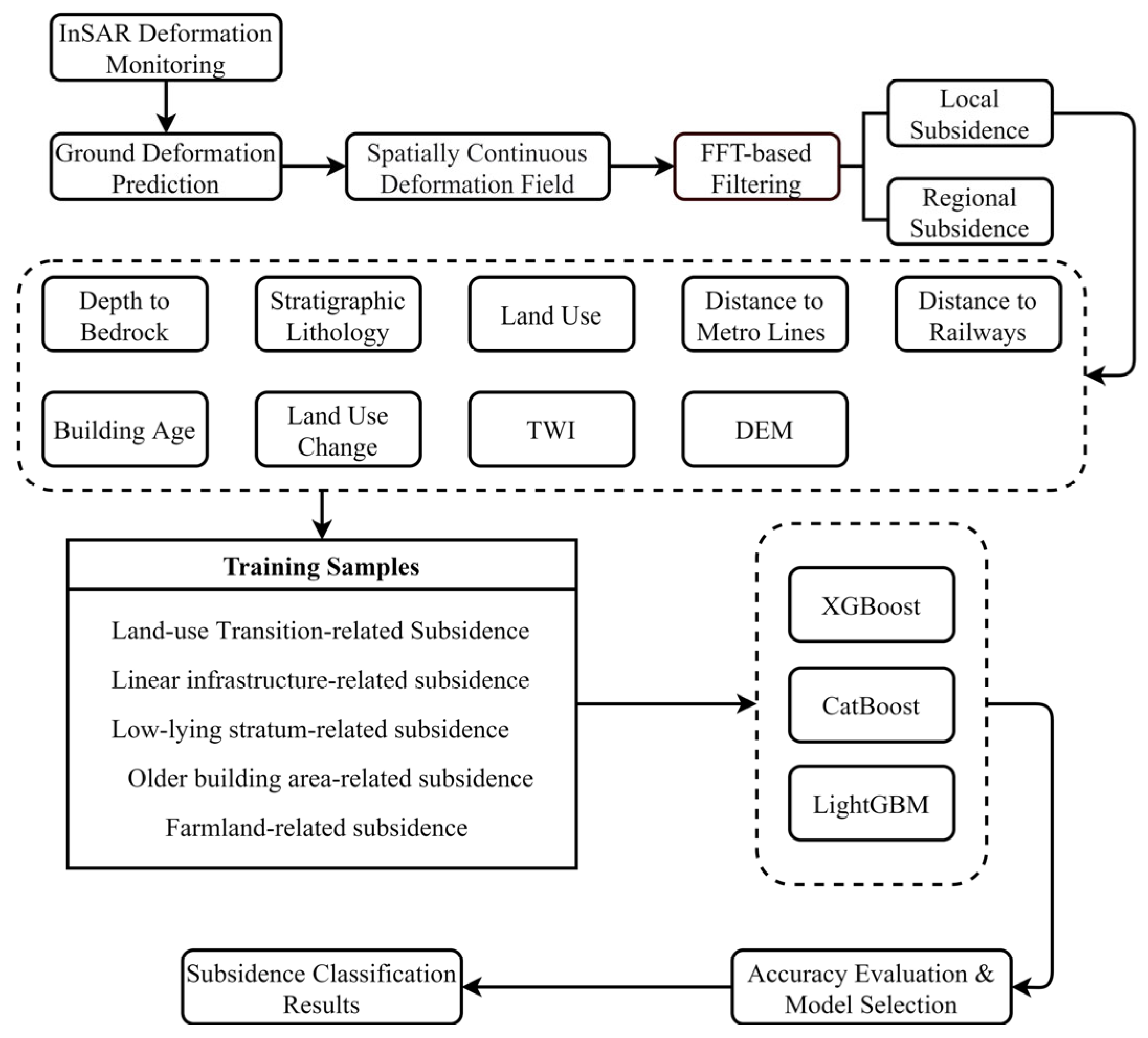
This study adopts a multi-stage methodological framework to achieve urban land subsidence type classification in Fuzhou. The framework consists of four sequential components: (1) retrieval of land subsidence deformation time series using time-series InSAR techniques; (2) generation of a spatially continuous deformation field through regression models to fill data gaps caused by decorrelation; (3) multi-scale decomposition of deformation signals to separate regional and local subsidence patterns; and (4) classification of local subsidence types using ensemble learning models combined with multi-source environmental and urban features. The overall methodological workflow is illustrated in Figure 1. Each methodological component is described in detail in the following subsections.

2.1. Study Area

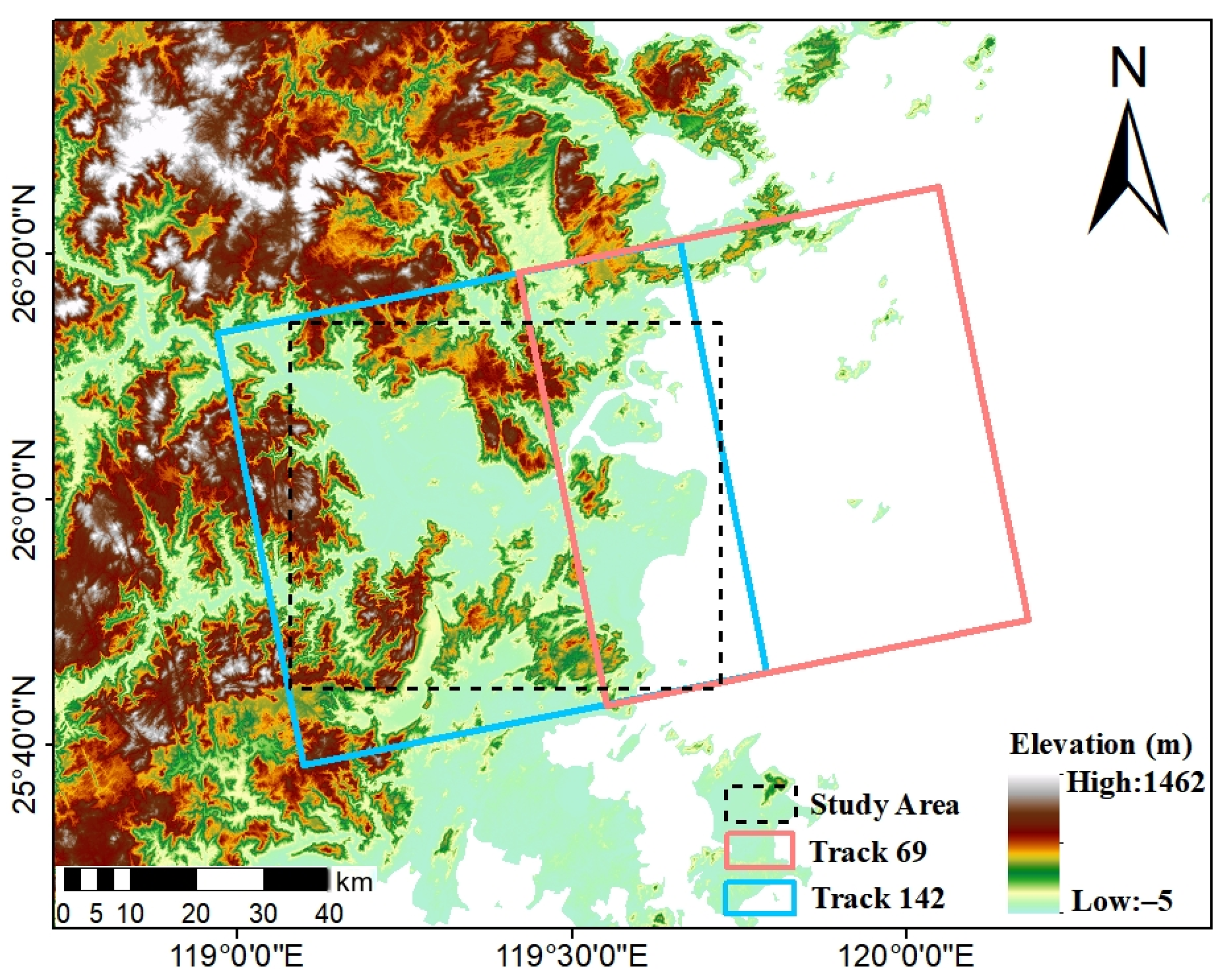
Fuzhou, located in eastern Fujian Province, is a typical coastal city situated within the sedimentary basin of the lower Min River and adjacent to the East China Sea and the Taiwan Strait (Figure 2). The region experiences a maritime subtropical monsoon climate and is characterized by unconsolidated geological formations and abundant groundwater resources. Together with rapid urban expansion and intensive transportation infrastructure development, these conditions render Fuzhou particularly susceptible to land subsidence. Long-term observations indicate that subsidence in Fuzhou has persisted for several decades. Leveling surveys recorded surface settlement in the Wenquan area as early as 1960–1990, followed by observation during 2008–2014, which identified six pronounced subsidence areas in the urban core, exhibiting an average subsidence rate of approximately −15 mm/yr and a maximum rate of −19.2 mm/yr [50]. Early investigations primarily focused on subsidence induced by geothermal water extraction [51,52]. However, similar to other coastal cities [53,54], accelerated urbanization, large-scale construction activities, including metro development and road construction [55], and continued groundwater exploitation [56] have substantially increased the complexity of subsidence drivers. As a result, the spatiotemporal evolution of land subsidence in Fuzhou has exhibited new and increasingly heterogeneous patterns [50].

2.2. InSAR Time-Series Deformation Retrieval

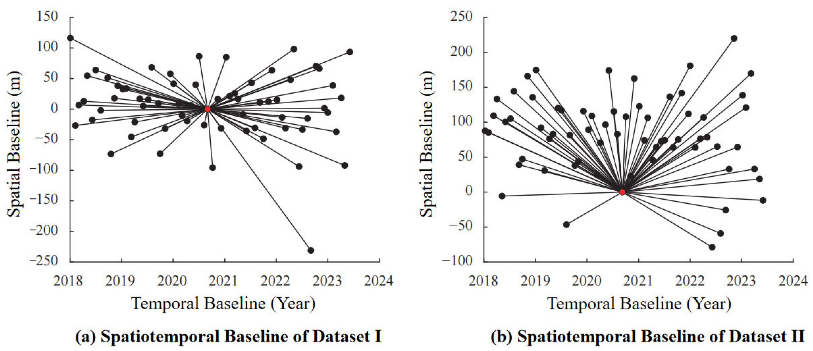
Two adjacent Sentinel-1A ascending tracks (Tracks 142 and 69), each consisting of 66 SAR scenes acquired between January 2018 and June 2023, were used to derive ground deformation information over Fuzhou (Figure 3). The results derived from Dataset I (Track 142) were used for the main deformation analysis, whereas Dataset II (Track 69) was used only for a cross-track consistency assessment within the overlapping area. This comparison evaluates the reproducibility of line-of-sight (LOS) deformation-rate patterns between two independently processed Sentinel-1 tracks.

Time-series InSAR processing was carried out to retrieve land subsidence deformation in the study area. Differential interferometric stacks were first generated using the InSAR Scientific Computing Environment (ISCE) software (version 2.5) [57]. Subsequently, deformation time series were estimated using Global Earth Observation Systems (GEOS)-Persistent Scatterer Interferometry (PSI), an in-house developed PSI processing framework implemented in MATLAB R2016b [12,58], which has been designed to enhance deformation estimation performance in complex urban environments.

The PSI analysis workflow adopted in this study can be summarized as follows. Persistent scatterer (PS) candidates were initially identified based on the amplitude dispersion index (ADI), with pixels satisfying ADI < 0.4 retained as candidates [8]. A high-quality subset of PS candidates (ADI < 0.25) was then selected to construct an initial reference network using a triangulation strategy. For each arc within the reference network, deformation model parameters were estimated using the least-squares ambiguity decorrelation adjustment (LAMBDA) method.

The reliability of the estimated parameters was evaluated using ensemble phase coherence, which provides a robust measure of phase stability across the interferometric stack [8]. Given the availability of a large number of SAR acquisitions, an ensemble coherence threshold of 0.65 was applied to ensure estimation reliability [59]. Spatial integration of the deformation parameters was subsequently performed using a robust fitting strategy (i.e., M-estimation) to derive the linear deformation and Digital Elevation Model (DEM) error of each measurement point. PS candidates not included in the initial reference network were progressively incorporated through an adaptive estimation procedure, allowing deformation information to be extended to a denser set of scatterers [12].

Following the initial linear estimation, orbital errors and atmospheric phase delays were iteratively estimated and removed using spatial–temporal filtering [60]. Subsequently, the remaining unmodeled deformation components were considered as non-linear deformation and were extracted from the unwrapped residual phases using spatial and temporal low-pass filtering. Finally, the linear deformation rates derived from the model and the estimated non-linear deformation were combined to generate complete deformation time series for each PS, while remaining residual signals not captured by these two components were treated as noise and excluded from the final deformation results.

The resulting displacement time series represent ground motion along the LOS direction. Accordingly, no direct LOS-to-vertical conversion was performed, and all subsequent reconstruction, FFT-based Butterworth filtering, and subsidence-type classification were conducted using LOS deformation rates. The broad deformation pattern was interpreted under a vertical-dominated subsidence hypothesis because several major processes considered in this study, particularly soft-soil consolidation, Quaternary sediment compaction, and construction loading, are generally expected to produce predominantly vertical settlement. However, this assumption does not imply that horizontal displacement is absent. Localized areas affected by metro excavation, riverbank deformation, engineered fills, slope instability, groundwater-pressure changes, or intensive construction activities may contain non-negligible horizontal motion. Because these components cannot be independently resolved from the available ascending-only observations, the deformation field should be interpreted as an LOS-based deformation product under a vertical-dominated subsidence hypothesis rather than as strictly decomposed vertical deformation.

2.3. Generation of a Spatially Continuous Deformation Field

Despite its robustness, PSI-based InSAR can suffer from decorrelation in areas with dense vegetation, low building density or pronounced surface changes, resulting in spatial gaps in the deformation field. To generate a spatially continuous deformation estimate for subsequent multi-scale spatial analysis, a regression-based reconstruction strategy [61,62] was adopted. The reconstructed field should be interpreted as a model-assisted estimate rather than a direct InSAR observation in decorrelated areas.

Twelve deformation-driving factors were selected as predictors, including distance to metro lines, distance to railways, digital elevation model (DEM), building height, topographic wetness index (TWI), lithology, land use, groundwater level, air temperature, normalized difference vegetation index (NDVI), depth to bedrock, and curvature.

Groundwater level observations from eight monitoring wells were obtained from the China Institute of Geo-Environment Monitoring. For use in the regression-based reconstruction of the continuous deformation field, the well observations were spatially interpolated using kriging to generate a groundwater level layer. Because the monitoring network was spatially sparse and information on well depth, screened aquifer, and groundwater-pumping volume was unavailable, the interpolated layer was treated as a broad hydrological predictor rather than direct evidence of groundwater-induced subsidence. To independently examine the temporal relationship between groundwater level variation and ground deformation, the original groundwater level observations were resampled to a daily interval. For each monitoring well, the mean LOS displacement time series of PS points located within a 150 m radius was extracted. The groundwater level and LOS-displacement records were aligned to common observation dates and examined using paired time-series comparison. This well-based analysis was conducted separately from the use of the interpolated groundwater level variable in the reconstruction model. The interpolated groundwater level layer was used only in the regression-based reconstruction of the continuous deformation field.

A systematic comparative analysis was conducted on three widely used regression models: XGBoost (version 2.1.3), LightGBM (version 4.5.0), and CatBoost (version 1.2.7). The regression models were constructed by integrating these predictors with InSAR-derived deformation rates, where the deformation rate was treated as the dependent variable and the selected factors as independent variables. The dataset was randomly partitioned into training (70%) and testing (30%) subsets to support model development and validation. The predictive capabilities of these models were evaluated using two primary metrics: coefficient of determination (R²) and root mean square error (RMSE).

The best-performing trained regression model (i.e., XGBoost in this work, see Section 3.1) was then applied on a pixel-by-pixel basis to estimate deformation values in decorrelated areas, producing a spatially continuous ground deformation field for the study area. The coherent-domain regression evaluation and visual comparisons between InSAR-derived and model-predicted deformation are presented in Section 3.1.

2.4. Multi-Scale Deformation Signal Decomposition

Ground deformation fields commonly contain components with different spatial wavelengths. Following previous studies, local subsidence generally refers to deformation features with relatively limited spatial extents, while regional subsidence corresponds to broader deformation areas [42]. In this study, the terms regional and local are used operationally to describe broad, low-spatial-frequency components and relatively localized, high-spatial-frequency components, respectively. These terms refer only to the spatial scale of the filtered signals and do not assign physical causes.

Broad low-frequency variations may mask localized deformation patterns and reduce their separability in subsequent classification. Therefore, the reconstructed deformation field was decomposed in the frequency domain before subsidence-type classification. The candidate classification domain was subsequently delineated from the extracted high-pass local component, as described below.

The input to the FFT procedure was the reconstructed LOS deformation-rate raster projected in WGS 84/UTM zone 50N. The raster contained 1832 rows and 2159 columns with a pixel spacing of 30 m × 30 m, corresponding to north–south and east–west extents of approximately 54.96 and 64.77 km, respectively. Non-finite pixels were assigned a value of zero to construct a complete numerical array, and the original valid-data mask was reapplied after inverse transformation. No additional padding or tapering window was used, and the original raster dimensions were retained throughout the procedure.

The LOS deformation-rate field f(x, y) was first transformed from the spatial domain into the frequency domain using a two-dimensional FFT (2D-FFT). The resulting spectrum was shifted to the center of the frequency domain as follows:

$${\mathrm{F}}_{\mathrm{c}}\left(\mathrm{u},\mathrm{v}\right)=\mathrm{fftshift}\left\{{\mathcal{F}}_2\left[\mathrm{f}\left(\mathrm{x},\mathrm{y}\right)\right]\right\}$$

(1)

A Butterworth high-pass filter was then used to extract high-frequency local deformation components. Its transfer function is expressed as:

$${\mathrm{H}}_{\mathrm{h}\mathrm{p}}\left(\mathrm{u},\mathrm{v}\right)={\displaystyle \frac{1}{1+{\left[\frac{{\mathrm{D}}_0}{\mathrm{D}\left(\mathrm{u},\mathrm{v}\right)}\right]}^{2\mathrm{n}}}}$$

(2)

where D(u, v) is the radial distance from spectral position (u, v) to the center of the shifted spectrum, D₀ is the radial cutoff radius in centered FFT index-coordinate units, and n is the Butterworth filter order. At D(u, v) = 0, the high-pass response was assigned a value of zero. The complementary low-pass filter was defined as:

$${\mathrm{H}}_{\mathrm{l}\mathrm{p}}\left(\mathrm{u},\mathrm{v}\right)=1-{\mathrm{H}}_{\mathrm{h}\mathrm{p}}\left(\mathrm{u},\mathrm{v}\right).$$

(3)

The Butterworth filter was selected because its gradual frequency response avoids the abrupt truncation associated with an ideal frequency-domain filter. Before inverse transformation, the filtered spectra were returned from the centered frequency arrangement to the original FFT ordering using ifftshift. The regional and local deformation components were reconstructed as:

$${\mathrm{V}}_{\mathrm{r}\mathrm{e}\mathrm{g}\mathrm{i}\mathrm{o}\mathrm{n}\mathrm{a}\mathrm{l}}\left(\mathrm{x},\mathrm{y}\right)=\mathrm{R}\mathrm{e}\left\{{\mathcal{F}}^{-1}\left[\mathrm{i}\mathrm{f}\mathrm{f}\mathrm{t}\mathrm{s}\mathrm{h}\mathrm{i}\mathrm{f}\mathrm{t}\left({\mathrm{F}}_{\mathrm{c}}(\mathrm{u},\mathrm{v}){\mathrm{H}}_{\mathrm{l}\mathrm{p}}(\mathrm{u},\mathrm{v})\right)\right]\right\},$$

(4)

$${\mathrm{V}}_{\mathrm{l}\mathrm{o}\mathrm{c}\mathrm{a}\mathrm{l}}\left(\mathrm{x},\mathrm{y}\right)=\mathrm{R}\mathrm{e}\left\{{\mathcal{F}}^{-1}\left[\mathrm{i}\mathrm{f}\mathrm{f}\mathrm{t}\mathrm{s}\mathrm{h}\mathrm{i}\mathrm{f}\mathrm{t}\left({\mathrm{F}}_{\mathrm{c}}(\mathrm{u},\mathrm{v}){\mathrm{H}}_{\mathrm{h}\mathrm{p}}(\mathrm{u},\mathrm{v})\right)\right]\right\}.$$

(5)

Only the real parts of the inverse FFT results were retained, and no additional post-filter smoothing or artifact-removal procedure was applied. Because the high- and low-pass filters were complementary, the sum of the reconstructed components reproduced the filled input field apart from numerical rounding errors.

Because D₀ is defined in centered FFT index-coordinate units, it does not correspond directly to a universal physical-distance, wavelength, or patch-area threshold. Its approximate physical scale depends on the raster dimensions and pixel spacing. The approximate axis-wise characteristic cutoff wavelengths can be expressed as:

$${\lambda }_{\mathrm{x}}\approx {\displaystyle \frac{{\mathrm{N}}_{\mathrm{x}}\Delta \mathrm{x}}{{\mathrm{D}}_0}},{\lambda }_{\mathrm{y}}\approx {\displaystyle \frac{{\mathrm{N}}_{\mathrm{y}}\Delta \mathrm{y}}{{\mathrm{D}}_0}},$$

(6)

where Nx and Ny are the numbers of columns and rows, respectively, and Δx and Δy are the corresponding pixel spacings. The baseline parameters were set to D₀ = 7 and n = 2, corresponding to approximate axis-wise characteristic cutoff wavelengths of 9.25 km in the east–west direction and 7.85 km in the north–south direction. Because the Butterworth response is gradual, D₀ controls the transition between the broad and localized components rather than defining a sharp spatial-scale boundary. A sensitivity analysis of D₀ and n was conducted to evaluate the influence of these parameter settings.

After the high-pass local deformation component was obtained, the local subsidence candidate area used for subsequent classification was defined as pixels with local deformation rates not greater than −2 mm/yr:

$${\mathsf{\Omega }}_{\mathrm{l}\mathrm{o}\mathrm{c}\mathrm{a}\mathrm{l}}=\left\{\left(\mathrm{x},\mathrm{y}\right)\left|{\mathrm{V}}_{\mathrm{l}\mathrm{o}\mathrm{c}\mathrm{a}\mathrm{l}}\left(\mathrm{x},\mathrm{y}\right)\le -2 \mathrm{m}\mathrm{m}/\mathrm{y}\mathrm{r}\right|\right\}$$

(7)

The −2 mm/yr value is a deformation-rate criterion used to define the spatial domain supplied to the classifier and should not be interpreted as a spatial-scale or patch-area threshold. Pixels containing invalid auxiliary variables were further removed before model prediction. Therefore, the final classification domain corresponds to the FFT-derived local subsidence candidate domain after auxiliary-data validity screening.

2.5. Feature Construction and Sample Labeling

In regression-based modeling, the target variable is continuous, and a large number of quantitative predictors are typically required to capture subtle variations in deformation magnitude. In contrast, the objective of the present classification task is to discriminate among different land subsidence types. Accordingly, feature selection in this study emphasizes variables that are diagnostically informative for distinguishing dominant subsidence-related types, rather than for directly predicting deformation rates.

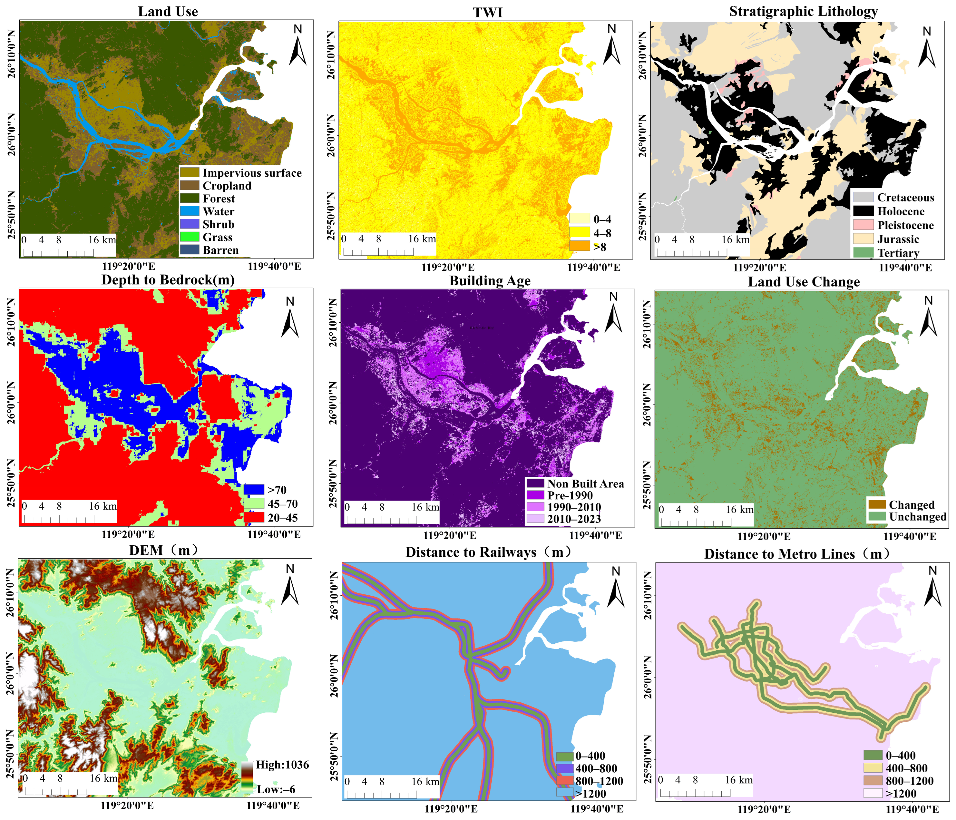
Based on this principle, a set of auxiliary features representing geological conditions, land-use characteristics, topographic attributes, and transportation infrastructure was constructed to support subsidence type classification. The spatial distributions of the selected features are shown in Figure 4.

2.5.1. Feature Construction

• Geological factors:

Stratigraphic lithology and depth to bedrock were used as broad contextual indicators of the geological setting. Lithological data at a scale of 1:200,000 were obtained from the National Geological Archives of China, and the depth-to-bedrock dataset had a native spatial resolution of 100 m [63]. They were used to characterize broad geological associations rather than to verify local stratum-compression or geotechnical mechanisms.

2.

Land use factors:

Land use information reflects both surface cover characteristics and the intensity of human activities. Urban expansion often involves the conversion of farmland, forests, and water bodies into impervious surfaces such as buildings and roads, increasing surface loading and altering soil structure, which may affect ground stability. In this study, a land-use transition matrix was constructed using multi-temporal land-use datasets to capture land-use change information. Building construction periods were further extracted to generate building age features.

The Code for Design of Building Foundations (GBJ 7-89) [64], first issued in 1989, introduced more stringent standards for foundation design and construction. Building construction period was used as a contextual building-age indicator. The year 1990 was retained as an operational temporal boundary for identifying older building areas in the available building-period dataset, rather than as an empirically validated threshold of foundation quality or settlement risk. The publication of a design code does not imply that foundation conditions changed abruptly after 1990. Therefore, the building-age variable was treated only as a contextual proxy for older building areas rather than as direct evidence of foundation-related settlement. Land-use data were obtained from the Zenodo platform at a spatial resolution of 30 m [65]. Land-use transition information was derived from 2010–2023 land-use datasets. The transition layer was used to characterize the broader land-development history and its spatial association with the mapped deformation. It should not be interpreted as direct evidence that a particular transition occurred during, or caused deformation within, the 2018–2023 InSAR observation period. Although delayed deformation following land development is possible, the timing and duration of such a response could not be quantified using the available land-use data.

3.

Topographic factors:

Topographic variables include the digital elevation model (DEM) and the topographic wetness index (TWI), which are used to identify low-lying areas with poor drainage conditions. A 30 m resolution Shuttle Radar Topography Mission (SRTM) DEM was employed, and sink filling was performed in ArcGIS Desktop (version 10.3) to generate a continuous and smooth elevation surface. TWI is a widely used index that quantifies the tendency of water accumulation and reflects the influence of topography on hydrological processes. It was calculated in ArcGIS based on the DEM as follows [66]:

$$\mathrm{T}\mathrm{W}\mathrm{I}=\ln \left({\displaystyle \frac{\mathrm{A}}{\mathrm{b}\tan \beta }}\right)$$

(8)

where A is the upslope contributing area, b is the grid cell width, and β is the local slope angle.

4.

Linear transportation infrastructure:

Distances to railways and metro lines were included as contextual proximity variables describing the spatial relationship between deformation and transportation corridors. The transportation-distance variables were used only as spatial contextual indicators and were not treated as evidence that transportation construction or operational loading caused the observed deformation.

2.5.2. Sample Labeling

To construct labeled samples for model training and validation, representative local subsidence patches were first identified from the local subsidence deformation map derived from the FFT-based Butterworth filtering. Patch boundaries were manually delineated according to the spatial continuity, deformation magnitude, and morphological coherence of local subsidence anomalies. A local subsidence patch was defined as a spatially contiguous deformation unit with relatively consistent deformation characteristics. Adjacent deformation areas were separated into different patches when clear discontinuities in the deformation field, differences in deformation morphology, or changes in dominant land-use, infrastructure, building-age, or geological/topographic conditions were observed. These candidate patches were then visually interpreted and labeled with the support of multi-source auxiliary information. The visual interpretation and initial label assignment were conducted by one interpreter. Historical imagery available in Google Earth Pro (version 7.3.6) was used primarily to examine observable surface-cover changes, construction activity, and infrastructure development, rather than to directly infer subsurface deformation mechanisms.

Only local subsidence patches with clear and consistent category characteristics were retained as labeled samples. Patches with insufficient evidence or ambiguous dominant characteristics were not included in the final labeled dataset. When multiple indicators overlapped within the same patch, the final label was assigned according to the dominant-type decision rule described below and summarized in

Table 1. Defining characteristics of five subsidence types considered in this study.

Subsidence Type	Main Characteristics	Dominant Labeling Criterion
Low-lying stratum-related subsidence	Occurs in Holocene and Pleistocene formations with large bedrock depth, low DEM, and high TWI	Assigned when geological and topographic indicators provide the dominant spatial context.
Linear infrastructure-related subsidence	Located close to railways, metro lines, or major transportation corridors	Assigned when the patch is spatially aligned with transportation corridors and shows belt-like deformation characteristics.
Older building area-related subsidence	Located in older building areas, identified using the pre-1990 construction period indicator	Assigned when older building areas dominate the patch and no stronger infrastructure-related or land-use transition evidence is observed.
Land-use transition-related subsidence	Occurs in areas spatially coinciding with significant land-use transition during urban development	Assigned when the local deformation patch coincides with clear land-use transition.
Farmland-related subsidence	Associated with agricultural land use	Assigned when the patch remains agricultural land and lacks clear evidence of construction or transportation disturbance.

.

It should be noted that the five classes used in this study represent dominant subsidence-related types rather than strictly mutually exclusive physical causes. In complex urban environments, multiple factors may coexist within the same subsidence patch. For example, farmland areas may also be located in low-lying soft strata, land-use transition areas may occur near roads or metro lines, and old building areas may also be underlain by compressible sediments.

When multiple indicators overlapped within the same patch, the dominant class was determined according to the diagnostic specificity, spatial coincidence, and deformation morphology of the available evidence. First, patches showing clear belt-like deformation spatially aligned with metro lines, railways, or major transportation corridors were labeled as linear infrastructure-related subsidence, when both belt-like deformation morphology and spatial alignment with transportation corridors were observed. Second, patches coinciding with evident land-use conversion were labeled as land-use transition-related subsidence when the deformation patch was spatially associated with newly developed or converted land rather than a narrow transportation corridor. Third, patches dominated by older building areas, identified using the pre-1990 construction-period indicator, were labeled as older building area-related subsidence when no stronger infrastructure-related or land-use transition evidence was observed. Fourth, patches that remained agricultural land and lacked clear evidence of construction or transportation disturbance were labeled as farmland-related subsidence. Finally, low-lying stratum-related subsidence was assigned when geological and topographic indicators, including Holocene or Pleistocene sediments, low elevation, high TWI, and large depth to bedrock, provided the dominant spatial context and no stronger anthropogenic evidence was identified. Patches for which no dominant class could be determined were excluded from the labeled dataset.

The final labeled dataset consisted of 467 manually delineated local subsidence patches. After rasterization at a spatial resolution of 30 m × 30 m, these patches collectively contained 6191 labeled grid cells. Each grid cell served as a model-sample unit with its own predictor values, while inheriting the dominant subsidence-related label assigned to the patch in which it was located. Therefore, the 467 patches represent the patch-level labeling units, whereas the 6191 rasterized grid cells represent the model-sample units. At the grid-cell level, the model-sample dataset included 955 land-use transition-related subsidence samples, 1668 farmland-related subsidence samples, 969 low-lying stratum-related subsidence samples, 2001 linear infrastructure-related subsidence samples, and 598 older building area-related subsidence samples.

The minimum mapping unit of the rasterized labeled data was one 30 m × 30 m grid cell, corresponding to 0.0009 km². The patch sizes calculated from the grid cells ranged from 0.0009 to 0.2682 km². To quantitatively describe the spatial distribution and spacing of the labeled patches, the centroid of each patch was calculated in the projected coordinate system. The patch centroids covered an east–west extent of approximately 56.1 km and a north–south extent of approximately 51.7 km within the study area, indicating that the labeled patches were not confined to a single local zone. The nearest-neighbor distance ranged from 0.0618 to 5.1668 km, with a mean value of 0.3848 km. These results indicate that the labeled patches include both spatially clustered local subsidence groups and more isolated patches, which is consistent with the spatially discontinuous nature of urban local subsidence.

2.6. Classification Models and Evaluation Protocol

2.6.1. Classification Models

To classify land subsidence types, three gradient boosting decision tree-based ensemble learning models, XGBoost, LightGBM, and CatBoost, were employed in this study. These models were selected due to their strong performance in handling nonlinear relationships, mixed feature types, and relatively small training datasets.

To reduce the influence of spatial autocorrelation associated with conventional random train-test splitting, a spatially stratified block-validation protocol was adopted for the classification task. The study area was divided into regular 3 km × 3 km spatial blocks, which were treated as indivisible grouping units. All labeled patches and rasterized grid-cell samples located within the same spatial block were assigned to the same fold, and all grid cells derived from the same manually delineated patch were retained in the same fold. Therefore, no spatial block or labeled patch contributed samples to both the training and testing subsets in the same validation iteration. The 3 km block size was adopted as a practical compromise between spatial separation and class-balance preservation. Smaller blocks would provide weaker separation among spatially neighboring samples, whereas larger blocks would reduce the number of available spatial groups and increase the risk of class under-representation in individual folds. The assignment of spatial blocks to folds was optimized to maintain similar class proportions across folds as far as possible. Five-fold spatial block cross-validation was then performed, with one group of spatial blocks held out for testing and the remaining groups used for training in each iteration.

Hyperparameter tuning was performed using the Optuna framework (version 4.1.0), which implements Bayesian optimization in combination with the Tree-structured Parzen Estimator (TPE) sampler [67]. The sampler seed was fixed at 42. Each model was assigned 100 completed trials, including 20 initial random trials. No trial pruning or model-specific timeout was applied. For each trial, model performance was evaluated using the same predefined 5-fold 3 km spatial block validation. All grid cells belonging to the same labeled patch and spatial block were retained in the same fold. The optimization objective was the mean macro-F1 across the five spatial validation folds. Macro-F1 was selected because it assigns equal importance to each class and is appropriate for the moderately imbalanced five-class classification problem.

Model-specific search spaces were defined because XGBoost, LightGBM, and CatBoost differ in their tree-growth strategies, parameter definitions, categorical-feature handling, and regularization mechanisms. Fairness was maintained by using the same labeled samples, input features, spatial folds, TPE settings, number of trials, and optimization objective for all three models. Identical numerical parameter values were not imposed because parameters with similar names may have different effects across the algorithms. Instead, parameters shared in function, including learning rate, tree depth, boosting iterations, row sampling, and feature sampling, were assigned comparable ranges where supported, while parameters unique to each algorithm were optimized within their respective model-specific spaces. Early stopping was not used because the number of boosting iterations was included in the optimization space. Class weights were not applied to any model. Instead, class imbalance was considered through the macro-F1 objective and was further assessed using balanced accuracy, weighted-F1, Cohen’s kappa, and class-wise metrics. The model-specific search spaces and final optimized configurations are summarized in

Table 2. Final selected model-specific hyperparameter settings.

Model	Search Space	Final Optimized Configuration
LightGBM	n_estimators: 100–1500, step 100; learning_rate: 0.01–0.20, log scale; max_depth: 3–10; num_leaves: 15–127; min_child_samples: 10–80; subsample: 0.70–1.00; colsample_bytree: 0.70–1.00; reg_alpha and reg_lambda: 0, 0.001, 0.01, 0.1, 1, or 10.	n_estimators = 500; learning_rate = 0.1; max_depth = 6; num_leaves = 31; min_child_samples = 20; subsample = 1.0; colsample_bytree = 1.0; reg_alpha = 0.0; reg_lambda = 0.0
XGBoost	n_estimators: 100–1500, step 100; learning_rate: 0.01–0.30, log scale; max_depth: 3–10; min_child_weight: 1–20; subsample: 0.70–1.00; colsample_bytree: 0.70–1.00; gamma: 0–1; reg_alpha: 0, 0.001, 0.01, 0.1, 1, or 10; reg_lambda: 0.01–20, log scale	n_estimators = 500; learning_rate = 0.3; max_depth = 6; min_child_weight = 1; subsample = 1.0; colsample_bytree = 1.0; gamma = 0.0; reg_alpha = 0.0; reg_lambda = 1.0;
CatBoost	iterations: 100–1500, step 100; learning_rate: 0.01–0.20; depth: 4–10; l2_leaf_reg: 0.01–20, log scale; random_strength: 0–10; border_count: 32, 64, 128, or 254; rsm: 0.70–1.00	iterations = 500; learning_rate = 0.1; depth = 6; l2_leaf_reg = 3; random_strength = 1; border_count = 254; rsm = 1.0

.

2.6.2. Evaluation Protocol

Model performance was evaluated using accuracy, balanced accuracy, macro-F1, weighted-F1, Cohen’s kappa, class-wise precision, class-wise recall, class-wise F1-score, receiver operating characteristic area under the curve (ROC-AUC) and precision-recall area under the curve (PR-AUC). Mean values and 95% confidence intervals were reported across the five spatial validation folds. The 95% confidence intervals were calculated using the t-distribution based on the 5-fold spatially stratified block validation results.

In addition, a label-permutation test was conducted under the same spatially stratified block validation protocol. The class labels were randomly permuted while the feature matrix and spatial folds were kept unchanged. This procedure was repeated 100 times, and the observed macro-F1 was compared with the permutation-based macro-F1 distribution. The permutation test was used as a diagnostic check to assess whether the observed classification performance was substantially higher than chance-level performance.

3. Results

3.1. InSAR Measurements

3.1.1. InSAR-Derived Deformation and Cross-Track Consistency

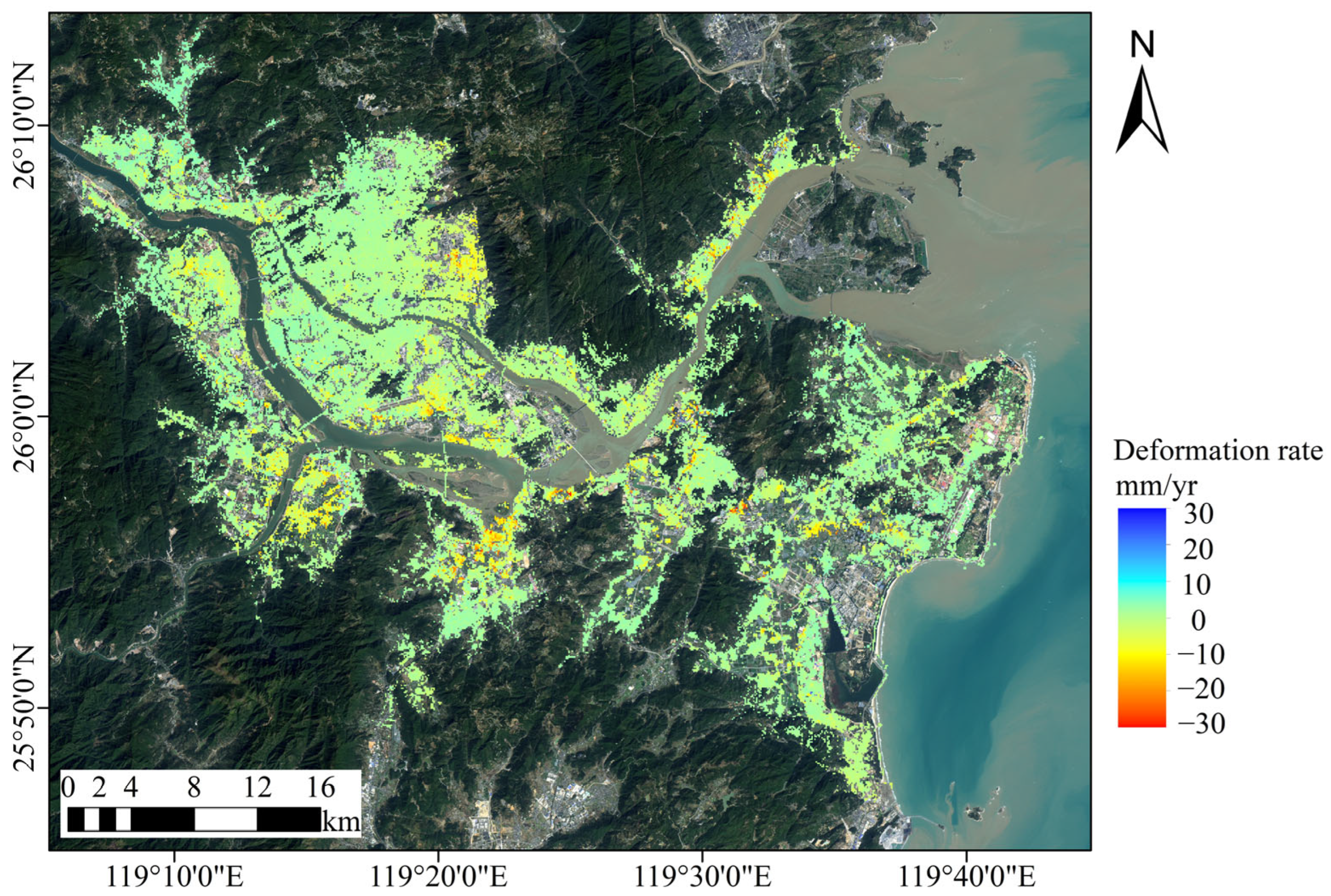
This approach was used to derive ground deformation velocity maps for the study area (Figure 5). A total of 980,078 PS points were identified in this study, with a mean deformation rate of −0.06 mm/yr and a standard deviation of 3.02 mm/yr. The results indicate that ground deformation in most parts of the study area remains stable, with 93.5% of the observation points exhibiting deformation rates lower than 5 mm/yr.

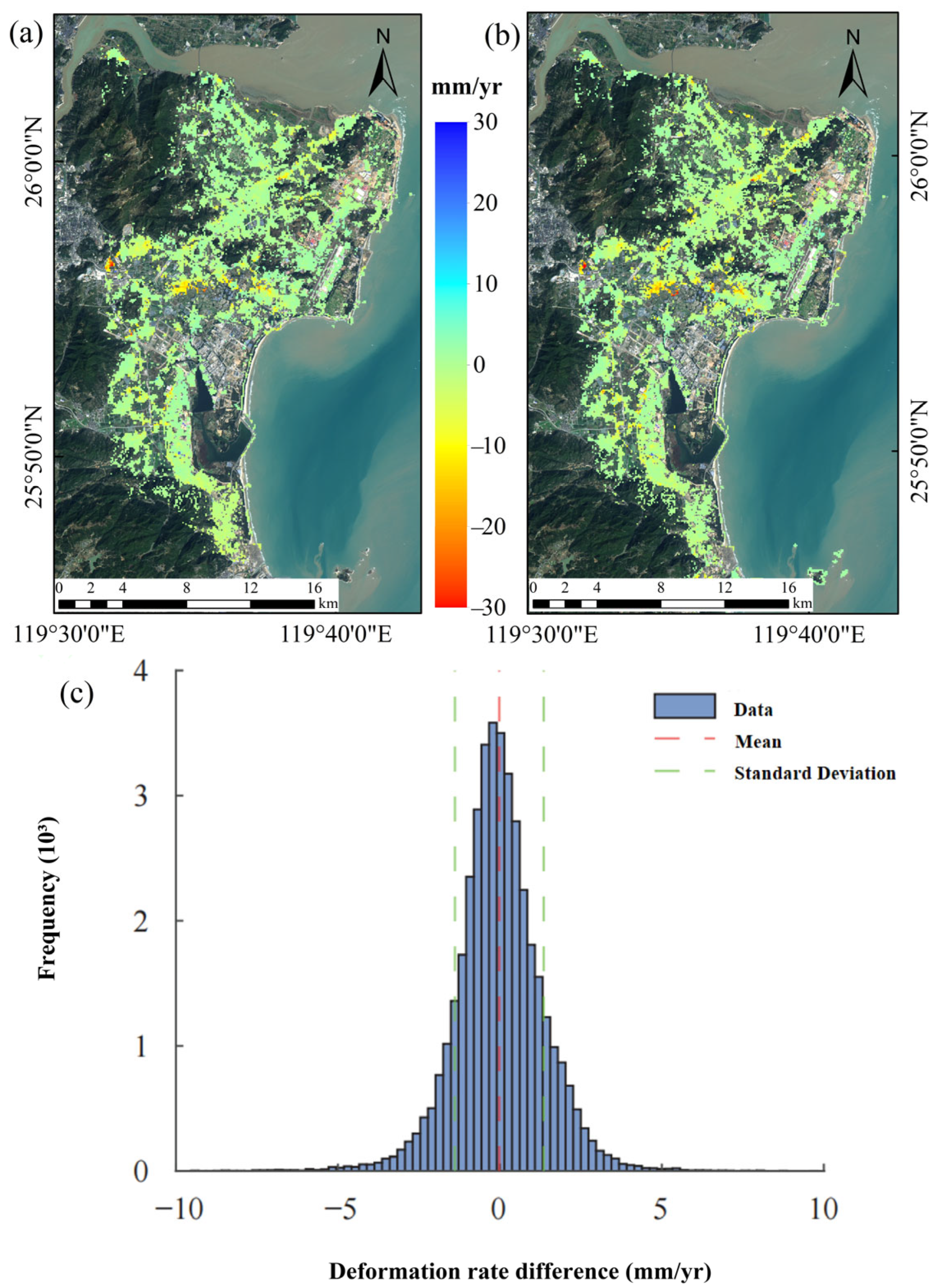
To assess the cross-track consistency of the InSAR-derived deformation results, a consistency analysis was conducted using LOS deformation rates from the overlapping areas of the two adjacent tracks. A total of 39,985 spatially collocated points were identified from Dataset I and Dataset II. Based on the deformation rates and their differences at these points, a histogram of the deformation rate difference distribution was plotted, as shown in Figure 6c. The results indicate that the discrepancies between the deformation rates derived from the two tracks are minor, with a standard deviation (Std) of 1.37 mm/yr. Notably, 88.08% of the points fall within the difference interval of −2 to 2 mm/yr. Furthermore, the Pearson correlation coefficient (R) between the two datasets was calculated to be 0.83. As detailed in

Table 3. Correlation statistics between Dataset I and Dataset II.

Statistics	Value
R	0.83
Std (mm/yr)	1.37
MSE (mm2/yr2)	1.98
RMSE (mm/yr)	1.41
MAD (mm/yr)	1.04

, root mean square error (RMSE) and mean absolute deviation (MAD) were both below 1.5 mm/yr, and mean square error (MSE) was 1.98 mm²/yr². These results demonstrate good cross-track consistency between the LOS deformation rates derived from the two adjacent ascending tracks. The comparison supports the reproducibility of the main spatial deformation pattern within the overlapping area. However, because both datasets were derived from Sentinel-1 observations and processed using the same PSI framework, the cross-track agreement should be interpreted as an internal consistency assessment rather than independent validation of absolute deformation accuracy. Potential common uncertainties associated with the reference point, atmospheric correction, orbital residuals, and LOS observation geometry may remain in both datasets.

3.1.2. Regression Evaluation and Deformation Reconstruction

The regression models were evaluated by comparing predicted deformation rates with withheld InSAR-derived measurements from spatially coherent areas. Therefore, the reported R² and RMSE quantify predictive fitting within the coherent-observation domain and do not directly evaluate reconstruction accuracy in genuinely decorrelated regions, where independent reference observations were unavailable.

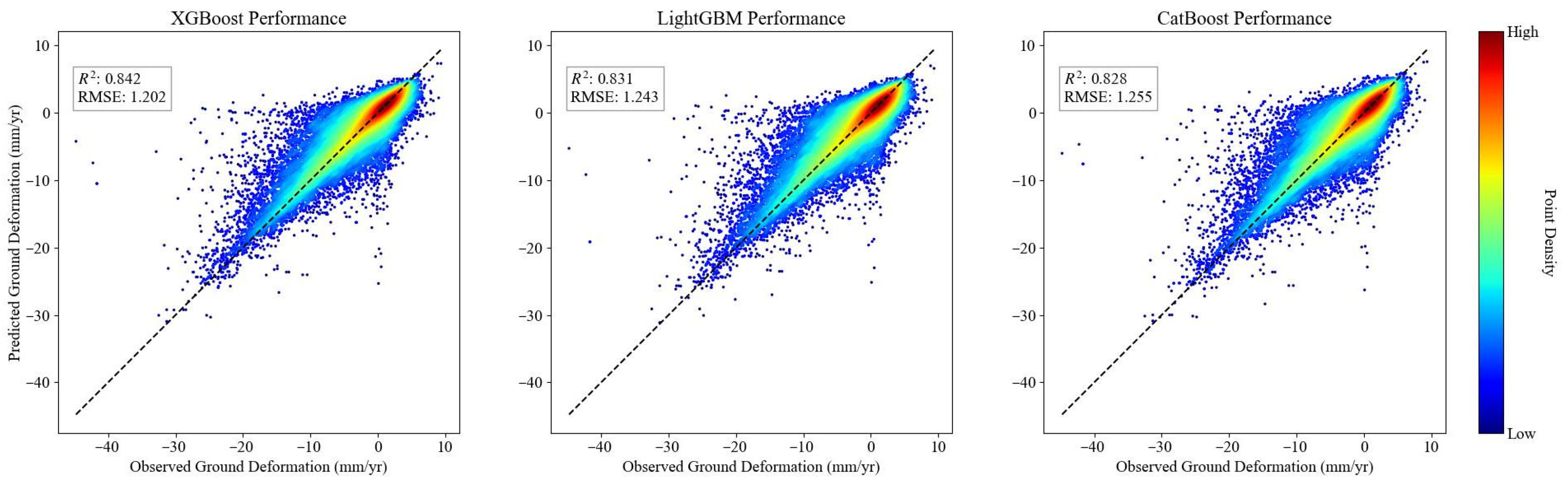
The results indicate that all regression models successfully capture the overall deformation pattern, and the simulated results show high consistency with the spatial distribution of the actual data. In terms of key metrics, all models achieved R² above 0.8 and RMSE below 2 mm/yr. These results indicate that the selected auxiliary predictors contain useful information for reproducing deformation-rate variations within the coherent-observation domain. However, they do not establish that these predictors represent the dominant physical controls on deformation.

However, a comparative analysis reveals that XGBoost achieved the best performance across both key metrics, with an R² of 0.842 and an RMSE of 1.202 mm/yr, outperforming the other two models. LightGBM followed with an R² of 0.831 and an RMSE of 1.243 mm/yr, showing intermediate coherent-domain test performance. CatBoost yielded an R² of 0.828 and an RMSE of 1.255 mm/yr; although slightly inferior to XGBoost, it showed similar but slightly lower coherent-domain test performance.

The distribution of predicted versus observed deformation rates on the 30% testing dataset for these models is further illustrated by scatter plots (Figure 7). In these plots, the color gradient represents the data point density, ranging from blue (low density) to red (high density), which shows a clear linear relationship with limited dispersion. Comprehensively considering all evaluation metrics, XGBoost demonstrates superior advantages in terms of coherent-domain fitting and predictive performance. Consequently, XGBoost was selected to generate the model-assisted continuous deformation estimate.

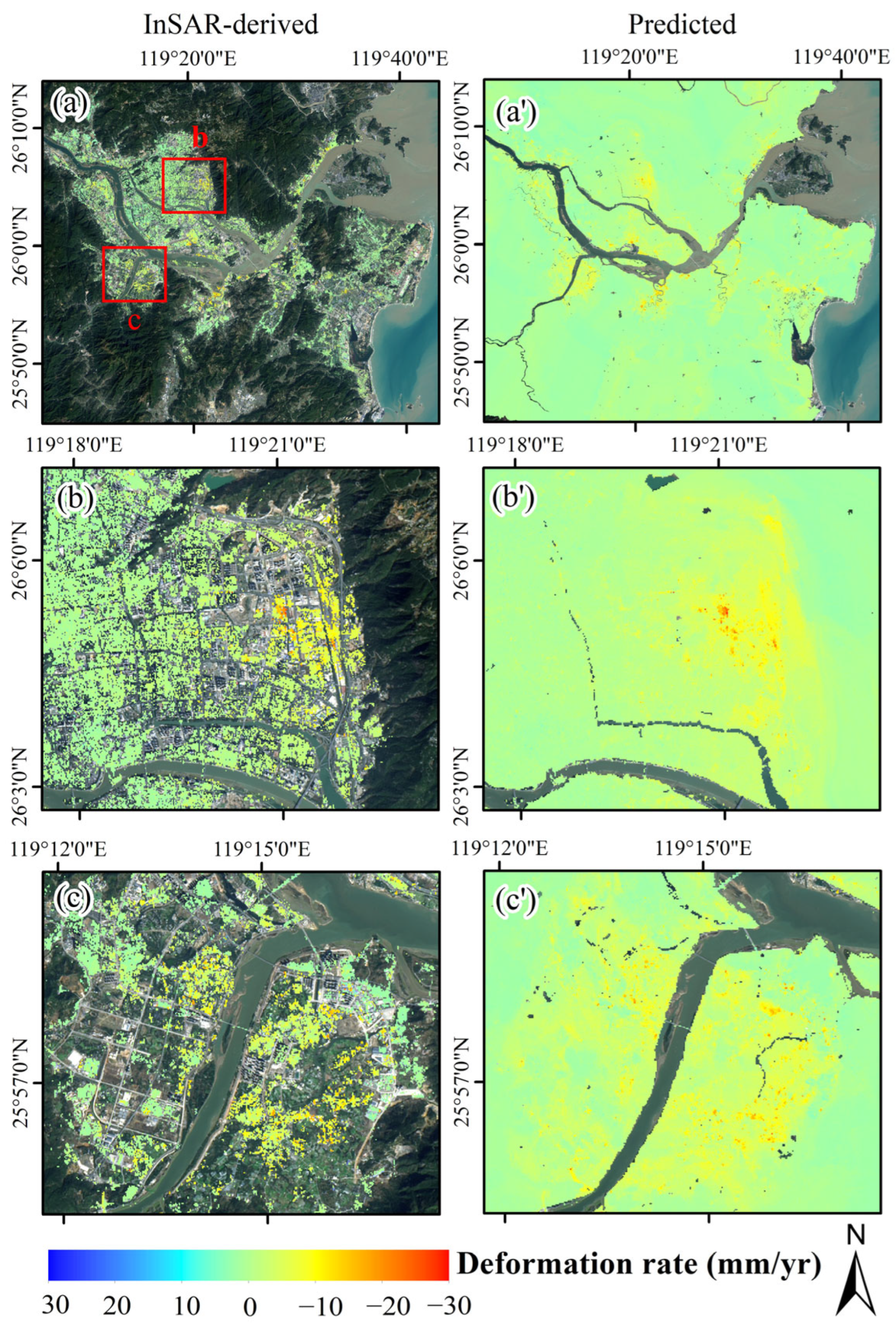
The trained model was subsequently applied on a pixel-by-pixel basis to estimate deformation values in decorrelated regions, producing a spatially continuous ground deformation field across the study area (Figure 8). Visual comparisons in two representative areas show smooth transitions and magnitude trends similar to those of adjacent coherent regions. These comparisons provide a qualitative continuity check.

Overall, the regression-based reconstruction provides a spatially continuous deformation estimate that is broadly consistent with deformation patterns in coherent areas. However, because independent observations are unavailable in truly decorrelated regions, this reconstructed field should be interpreted as a model-assisted estimate rather than a directly validated deformation product.

3.1.3. Groundwater Variations and Relationship with Deformation

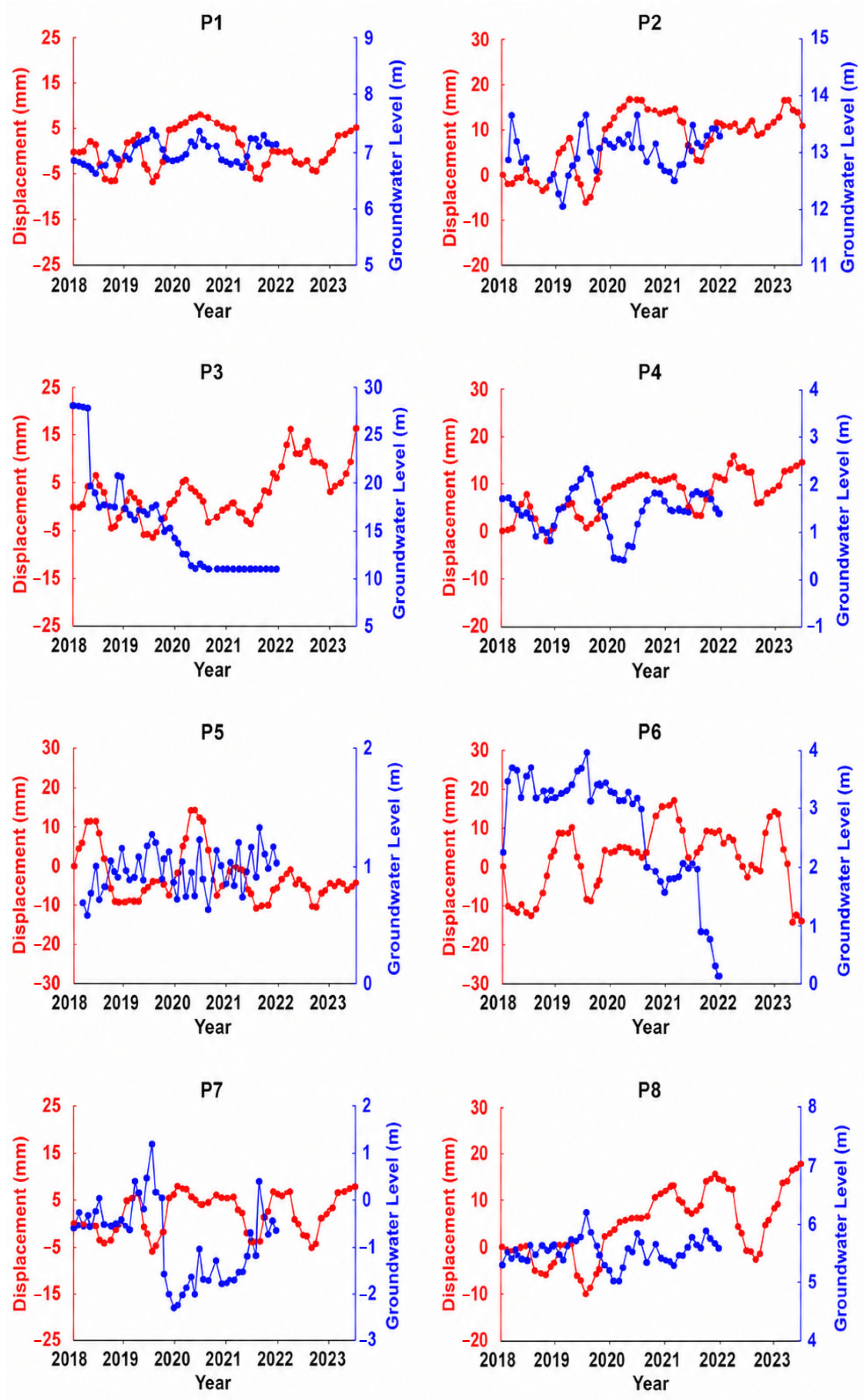
Groundwater level observations from the eight monitoring wells were visually compared with the mean LOS-displacement time series of surrounding PS points. The groundwater level at most wells showed relatively small or oscillatory variations rather than a consistent long-term decline. The paired time-series plots did not reveal a clear and consistently observable temporal correspondence between groundwater level variation and LOS displacement at the monitored locations. However, this qualitative comparison does not constitute a statistical test of correlation and does not account for possible delayed, nonlinear, or aquifer-specific responses. As shown in Figure 9, the groundwater level fluctuation ranges at P1 and P5 were relatively small, at 0.76 and 0.73 m, respectively. Larger but predominantly oscillatory variations were observed at P2, P4, and P8, with ranges of 1.61, 1.93, and 1.18 m, respectively. The differences between their initial and final groundwater levels were only 0.39, 0.30, and 0.28 m. An abrupt decrease of approximately 8 m was recorded at P3 within one month; because this observation could not be independently verified, it was treated as potentially anomalous and was not used as evidence of a regional groundwater trend.

These results did not reveal a clear and consistently strong temporal correspondence between groundwater level variation and LOS displacement at the monitored locations. Overall, the available records did not show a consistent long-term groundwater level decline across the monitored wells corresponding to the observed deformation. This result applies only to the available well locations and should not be generalized to exclude groundwater effects throughout Fuzhou.

3.2. Multi-Scale Deformation Characteristics After Decomposition

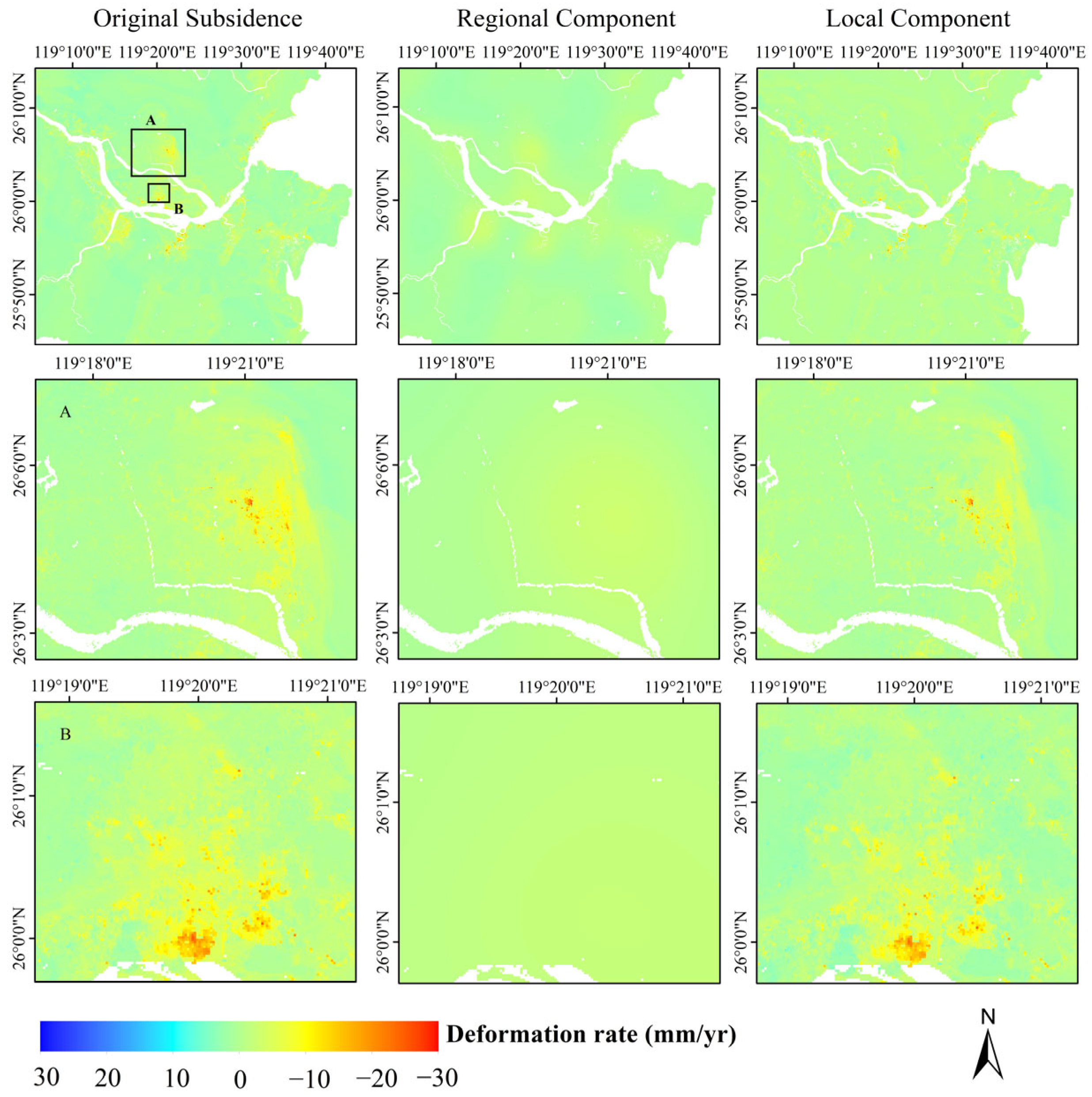
To examine deformation characteristics at different spatial scales, the reconstructed continuous deformation field was decomposed into broad low-spatial-frequency and localized high-spatial-frequency components using the FFT-based Butterworth filtering procedure described in Section 2.4. Figure 10 shows the original deformation field, the low-pass regional component, and the high-pass local component, together with enlarged views of representative areas A and B.

As shown in the first row of Figure 10, the original deformation field contains broad, smoothly varying signals superimposed with localized deformation features. The low-pass regional component preserves the broad spatial trends and smooth deformation gradients while suppressing high-spatial-frequency variations. It is mainly distributed along low-lying coastal areas and major river corridors. Although this distribution is spatially consistent with the geological and hydrogeological context of the study area, such correspondence is contextual and should not be interpreted as assigning a physical cause to the low-frequency component.

The high-pass local component shows spatially localized deformation features with sharper boundaries and greater spatial variability. The enlarged views of areas A and B demonstrate that frequency decomposition enhances localized features that are partly masked by broad background variations in the original deformation field. However, these high-spatial-frequency features should not be interpreted as direct evidence of infrastructure-, building-, or land-use-related physical mechanisms.

To evaluate the robustness of the FFT-based Butterworth filtering parameters, a sensitivity analysis was further conducted by varying the radial cutoff parameter D₀ and the Butterworth filter order n. Radial cutoff values of D₀ = 5, 7, 9, and 11, and filter orders of n = 1, 2, and 3, were tested. The same −2 mm/yr deformation-rate criterion was applied to every parameter combination when delineating the local subsidence candidate domain.

The sensitivity analysis shows that the continuous local deformation component was highly stable across the tested parameter settings. The spatial correlation between each tested local component and the baseline local component ranged from 0.976 to 1.000, and the RMSE remained lower than 0.267 mm/yr. This indicates that the main local deformation intensity field was robust to moderate changes in D₀ and n. In contrast, the thresholded local subsidence candidate area showed moderate sensitivity to parameter settings, with extracted areas ranging from 86.253 to 125.654 km² and intersection over union (IoU) values ranging from 0.789 to 1.000. This sensitivity mainly occurred along marginal pixels and patch boundaries near the −2 mm/yr threshold.

Table 4. Results of the sensitivity analysis for FFT-based Butterworth filtering parameters.

Parameter	Tested Value	Candidate Area (Mean ± SD km2)	Correlation with Baseline	RMSE Relative to Baseline (mm/yr)	IoU with Baseline
Radial cutoff parameter (D0)	5	122.908 ± 3.585	0.986	0.217	0.839
	7	105.986 ± 1.583	0.998	0.062	0.961
	9	95.566 ± 1.469	0.992	0.156	0.871
	11	88.194 ± 1.775	0.981	0.242	0.796
Filter order (n)	1	100.795 ± 14.097	0.990	0.181	0.855
	2	103.918 ± 15.459	0.991	0.146	0.880
	3	104.778 ± 15.620	0.988	0.180	0.865
Baseline setting	D0 = 7, n = 2	106.796	1.000	0.000	1.000

reports parameter-wise averaged results for each radial cutoff parameter and filter order.

Among the tested parameters, the radial cutoff parameter D₀ had a stronger influence than the Butterworth filter order n. A smaller D₀ retained more medium-scale deformation in the high-pass component and produced a larger candidate area, whereas a larger D₀ assigned more medium-scale signals to the regional component and reduced the extracted local subsidence candidate area. The influence of n was relatively weaker. Considering the high stability of the continuous local deformation field and the intermediate candidate-domain extent under the tested parameter range, D₀ = 7 and n = 2 were retained as the baseline configuration.

For each radial cutoff parameter D₀, the values are averaged over filter orders n = 1, 2, 3. For each filter order n, the values are averaged over radial cutoff values D₀ = 5, 7, 9, 11. The candidate area refers to pixels with V_local (x, y) ≤ −2 mm/yr before auxiliary-feature validity screening. The final classified area reported in Figure 11 is 105.596 km² after removing pixels with invalid auxiliary variables.

Overall, the FFT-based Butterworth filtering decomposed the continuous deformation field into a broad regional background component and a local high-frequency component. The local subsidence candidate area derived from the high-pass component was subsequently used as the classification domain, allowing the classifier to focus on spatially localized deformation while reducing the influence of broad background variations. This decomposition is operational and should not be interpreted as evidence that the filtered components correspond to distinct physical mechanisms.

3.3. Classification Results of Land Subsidence Types

Based on the local subsidence component extracted through FFT-based Butterworth filtering (Section 3.2), ensemble learning models were applied to classify dominant subsidence-related types across the study area. The classification was performed using three gradient boosting decision tree models—LightGBM, XGBoost, and CatBoost—trained on the labeled local subsidence samples described in Section 2.5.2. This section presents a comparative evaluation of model performance and the spatial classification results derived from the optimal model.

3.3.1. Model Performance Comparison and Optimal Model Selection

The classification performance of the three ensemble learning models was evaluated using a 5-fold spatially stratified block validation.

Table 5. Comparison of classification performance for land subsidence types using different models. Values are reported as mean ± 95% confidence interval across the five spatial validation folds.

Model	Accuracy	Balanced Accuracy	Macro-F1	Weighted-F1	Cohen’s Kappa
LightGBM	0.816 ± 0.083	0.813 ± 0.076	0.817 ± 0.070	0.815 ± 0.086	0.758 ± 0.112
XGBoost	0.805 ± 0.090	0.809 ± 0.081	0.810 ± 0.075	0.805 ± 0.094	0.744 ± 0.121
CatBoost	0.801 ± 0.078	0.811 ± 0.076	0.807 ± 0.069	0.799 ± 0.084	0.739 ± 0.106

summarizes the overall classification performance of the three models under the 3 km spatially stratified block validation.

Among the three models, LightGBM achieved the best overall classification performance. The best LightGBM setting obtained the highest accuracy, macro-F1, weighted-F1, and Cohen’s kappa, with values of 0.816, 0.817, 0.815, and 0.758, respectively. XGBoost showed comparable performance, with a macro-F1 of 0.810 and a Cohen’s kappa of 0.744. CatBoost achieved slightly lower accuracy and macro-F1 than LightGBM and XGBoost.

At the class level, the three models showed broadly similar performance patterns (

Table 6. Class-wise classification performance of the model configurations.

Model	Metric	Subsidence Category
		Farmland- Related	Low-Lying Stratum- Related	Linear Infrastructure- Related	Older Building Area- Related	Land-Use Transition-Related	Macro Average
LightGBM	Precision	0.845	0.723	0.798	0.947	0.825	0.828
	Recall	0.719	0.672	0.939	0.935	0.801	0.813
	F1-score	0.777	0.696	0.862	0.941	0.813	0.818
	ROC-AUC	0.949	0.940	0.967	0.993	0.976	0.965
	PR-AUC	0.878	0.764	0.923	0.980	0.898	0.889
XGBoost	Precision	0.823	0.691	0.799	0.941	0.820	0.815
	Recall	0.697	0.671	0.914	0.940	0.818	0.808
	F1-score	0.755	0.681	0.853	0.941	0.819	0.809
	ROC-AUC	0.936	0.934	0.962	0.989	0.977	0.960
	PR-AUC	0.851	0.758	0.914	0.972	0.884	0.876
CatBoost	Precision	0.820	0.676	0.795	0.941	0.816	0.809
	Recall	0.683	0.634	0.900	0.963	0.866	0.809
	F1-score	0.745	0.654	0.844	0.952	0.840	0.807
	ROC-AUC	0.947	0.935	0.964	0.995	0.978	0.964
	PR-AUC	0.876	0.752	0.920	0.982	0.899	0.886

). Class-wise precision, recall, and F1-score were calculated from the confusion matrix pooled across all out-of-fold predictions. The macro-average is the unweighted mean across the five classes and may therefore differ slightly from the mean of the fold-wise macro-F1 values reported in Table 5. Older building area-related subsidence was the most reliably identified category for all models, with F1-scores of 0.941, 0.941, and 0.952 for LightGBM, XGBoost, and CatBoost, respectively. Linear infrastructure-related subsidence also showed relatively high F1-scores, ranging from 0.844 to 0.862. These results indicate that older building area-related and infrastructure-related subsidence types have relatively distinct feature characteristics under the adopted multi-source geospatial feature space.

In contrast, low-lying stratum-related subsidence showed the lowest F1-score across all three models, with values of 0.696 for LightGBM, 0.681 for XGBoost, and 0.654 for CatBoost. Farmland-related subsidence also showed relatively lower recall than the other categories, with recall values of 0.719, 0.697, and 0.683 for LightGBM, XGBoost, and CatBoost, respectively. This indicates that a considerable proportion of farmland-related subsidence samples were misclassified into other categories. The main misclassifications occurred among farmland-related subsidence, low-lying stratum-related subsidence, and linear infrastructure-related subsidence. This pattern is reasonable because agricultural land, low-lying compressible strata, and transportation corridors may spatially overlap in urbanizing coastal areas.

The class-wise ROC-AUC and PR-AUC values provide additional information on model probability-ranking ability. All three models achieved high ROC-AUC values across the five classes, suggesting that the predicted probabilities generally separated each class from the remaining classes under the one-versus-rest evaluation. LightGBM achieved the highest ROC-AUC values for farmland-related, low-lying stratum-related, and linear infrastructure-related subsidence, whereas CatBoost achieved the highest values for older building area-related and land-use transition-related subsidence. The differences among the models were generally small. The PR-AUC results showed a pattern consistent with the F1-score results. Older building area-related subsidence achieved the highest PR-AUC values, whereas low-lying stratum-related subsidence had the lowest PR-AUC values across all three models. This further confirms that low-lying stratum-related subsidence was the most difficult category to distinguish. Considering the overall spatial validation performance and model stability, LightGBM was selected as the preferred model for classification of land subsidence types.

For the selected LightGBM configuration, the permutation test further suggested that the observed performance was substantially higher than chance-level performance under the same spatial validation protocol. The observed macro-F1 was 0.8174, whereas the mean macro-F1 from 100 randomly permuted labels was 0.1852, with a permutation p-value of 0.0099. However, this result should be interpreted as diagnostic evidence of non-random classification performance rather than definitive proof that label-rule dependence was completely absent.

The models showing the highest mean performance differed between the two tasks. For deformation reconstruction, which was formulated as a continuous regression problem, XGBoost achieved the highest R² and the lowest RMSE among the evaluated models. For subsidence type classification, LightGBM achieved the highest mean accuracy, macro-F1, weighted-F1, and Cohen’s kappa under the adopted spatial block cross-validation. However, the differences among the three classifiers were relatively small, and their confidence intervals overlapped substantially. Therefore, the results do not demonstrate the general superiority of XGBoost for regression or LightGBM for classification. Instead, they indicate that relative model performance in this study depended on the task formulation, response variable, sample structure, feature representation, hyperparameter optimization, and adopted evaluation procedure. XGBoost was consequently selected for deformation reconstruction, whereas LightGBM was selected to generate the reference subsidence type map, based only on their respective empirical performance in the present datasets.

3.3.2. Spatial Distribution of Land Subsidence Types

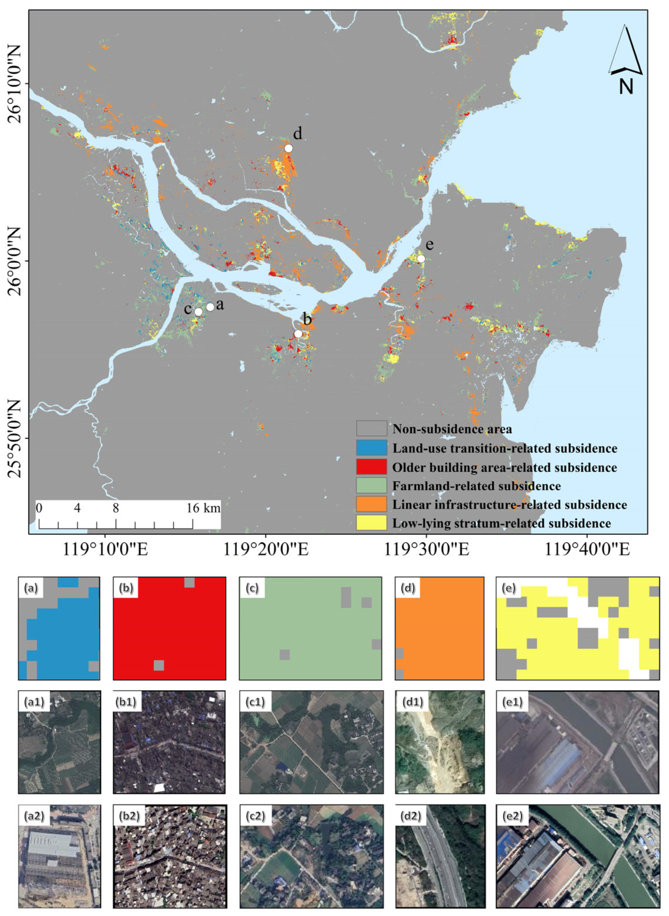
After model comparison using 5-fold spatially stratified block validation, LightGBM was selected as the final classifier and retrained using the complete labeled sample set. The classification results show pronounced spatial heterogeneity in the mapped dominant subsidence types. Figure 11 presents the spatial distribution of the five subsidence types, together with representative local examples showing their typical surface and spatial contexts. Google Earth historical imagery from 2010 and 2023 was used to illustrate observable changes in land use, construction activity, and the surrounding surface environment. At the selected locations, the observable surface characteristics and temporal changes shown in the historical imagery were visually consistent with the characteristics associated with the subsidence types. 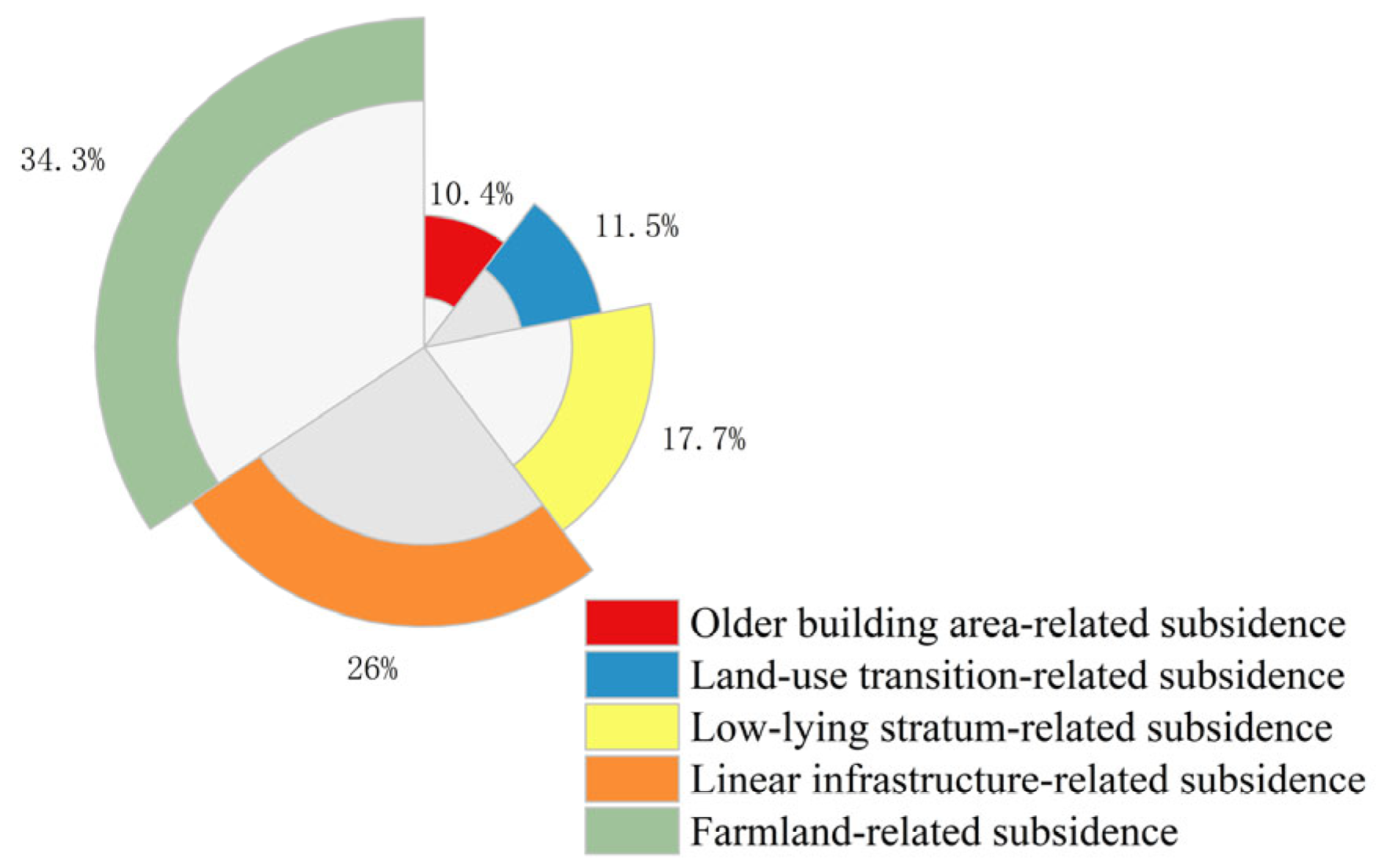The area proportions of the five subsidence types are summarized in Figure 12. These area proportions were calculated from one reference LightGBM classification map under the specific filtering configuration and should be interpreted as conditional summaries.

Farmland-related subsidence occupies the largest proportion of the total subsidence area, accounting for 34.3% (36.26 km²), and is mainly distributed in agricultural land located in suburban and peri-urban areas surrounding the urban core.

Linear infrastructure-related subsidence constitutes a relatively large proportion of the total subsidence area, accounting for 26% (27.41 km²), and exhibits a wide spatial distribution. This type of subsidence is primarily aligned with major urban roads, railways, and metro lines, and is particularly prominent in the urban core and surrounding areas with dense infrastructure. These patterns are spatially associated with areas of rapid urban development and transportation-network expansion. A typical example is located in Gushan Town, Jin’an District, where multiple railway and metro lines intersect. As illustrated in Figure 11(d–d2), the enlarged area is located near the Airport Expressway and Wenfu Railway in Gushan Town. This example illustrates the spatial correspondence between belt-like deformation and transportation corridors.

Low-lying stratum-related subsidence accounts for 17.7% (18.74 km²) of the total subsidence area and is mainly distributed in coastal zones, riverbanks, and low-elevation regions, such as the Min River estuary and its adjacent areas. As shown in Figure 11(e–e2), a representative area is located in Hangcheng Subdistrict, Changle District, on both sides of a Min River distributary, where low elevation and high topographic wetness index values are observed.

Land-use transition-related subsidence represents 11.5% (12.18 km²) of the total subsidence area and exhibits a relatively scattered spatial distribution. This mapped type is spatially associated with areas undergoing urbanization and land-use transition and is particularly evident in newly developed areas such as Nanyu Town, Nantong Town, and Shangjie Town in Minhou County. In these areas, agricultural land or natural surfaces have gradually been converted into impervious built-up land. As illustrated in Figure 11(a–a2), the representative site in Nantong Town transitioned from extensive farmland in 2010 to construction land by 2023.

Older building area-related subsidence occupies the smallest area proportion, accounting for 10.4% (11.01 km²) of the total subsidence area. This type is characterized by a fragmented spatial pattern and is mainly concentrated in locations such as Luozhou Town in Cangshan District and Shanggan Town in Minhou County. This mapped category is concentrated mainly in older building areas. Building construction period was used as a contextual age indicator. The 1990 boundary should not be interpreted as an abrupt change in foundation quality or as an empirically validated settlement-risk threshold. Therefore, this category should be interpreted as an older building area-related spatial type. As shown in Figure 11(b–b2), the enlarged example from Shanggan Town reveals a densely built and historically developed area that remained urban land throughout the 2010–2023 period.

3.4. Subsidence Rate Characteristics of Different Subsidence Types

Following the spatial classification of land subsidence types obtained using the optimal LightGBM model (Section 3.3), the deformation rate characteristics associated with each subsidence type were further examined. To this end, the classified subsidence map was spatially overlaid with the reconstructed continuous LOS deformation-rate field, and subsidence rates were statistically analyzed for each subsidence category. The resulting deformation rate distributions are conditional on the same reference LightGBM classification map and should not be interpreted as uncertainty-bounded estimates. 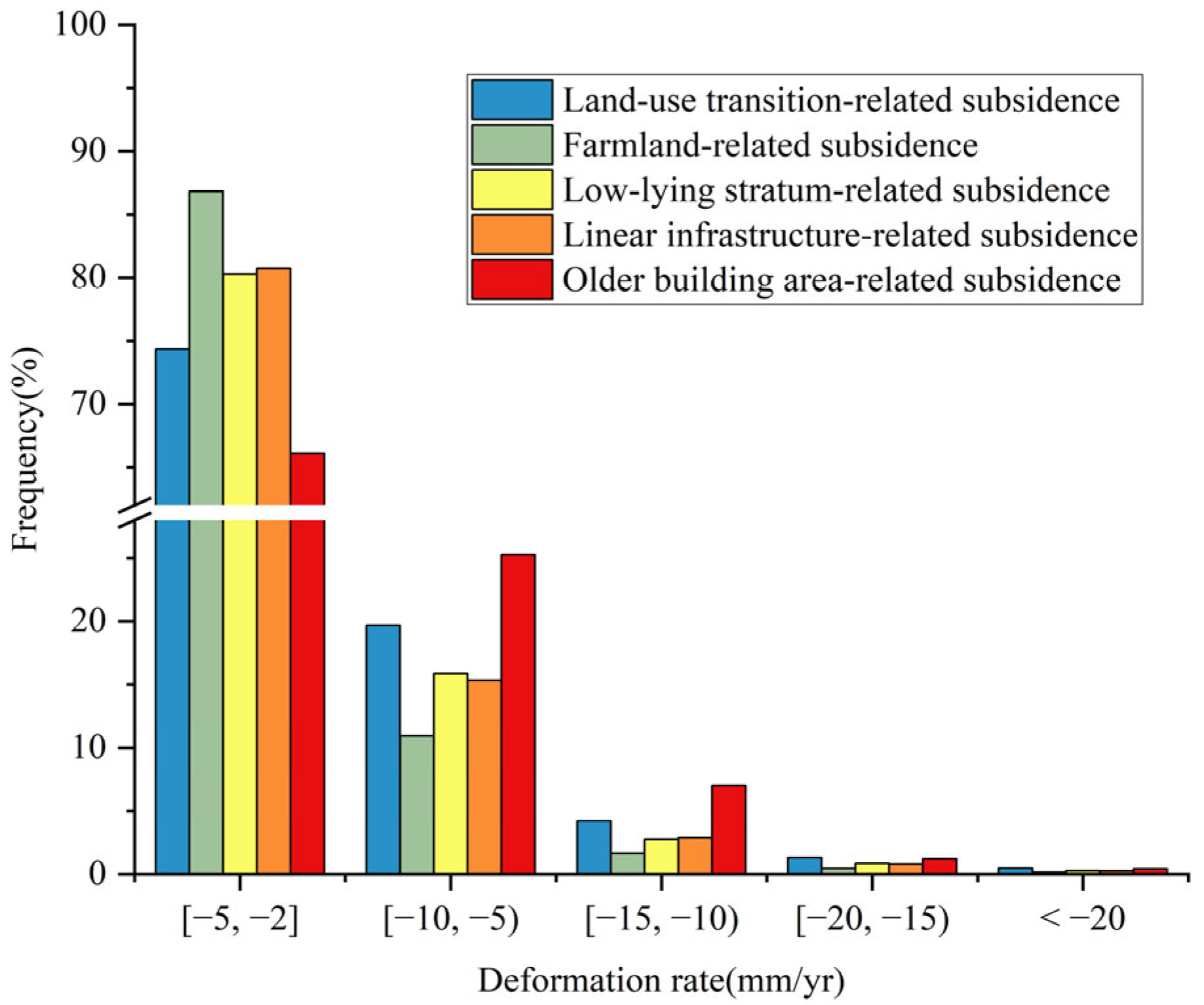Figure 13 illustrates the frequency distributions of subsidence rates for the five identified subsidence types across different deformation rate intervals. The results reveal clear differences in subsidence rate characteristics among the subsidence categories, showing that the five mapped categories exhibit different deformation-rate distributions.

Farmland-related subsidence is predominantly concentrated in lower deformation rate intervals, particularly between −5 and −2 mm/yr. Although this subsidence type occupies the largest spatial extent among all categories, its deformation rates are generally moderate, and the frequency of occurrence decreases substantially in higher subsidence rate intervals. This suggests that farmland-related subsidence is mainly characterized by slow and relatively uniform ground settlement.

In contrast, older building area-related subsidence and land-use transition-related subsidence exhibit a markedly different pattern. Despite their smaller spatial extents, these two subsidence types account for the highest proportions within severe subsidence rate intervals (<−10 mm/yr). Their deformation rate distributions show a pronounced rightward shift toward higher absolute values, indicating a tendency toward rapid and localized ground deformation.

Linear infrastructure-related subsidence displays an intermediate behavior. While its overall spatial extent is second only to farmland-related subsidence, its frequency within higher subsidence rate intervals is notably greater than that of farmland-related subsidence and comparable to that of older building area-related subsidence. This indicates that the mapped areas spatially associated with transportation corridors include both moderate and relatively high deformation rates.

Low-lying stratum-related subsidence exhibits a relatively balanced deformation rate distribution. Its frequency across moderate and higher subsidence rate intervals is comparable to that of linear infrastructure-related subsidence. This distribution indicates a spatial association with low-elevation areas characterized by the available broad-scale geological and geomorphological indicators.

4. Discussion

4.1. Limitations and Future Directions

4.1.1. Interpretation Scope and Independent Validation

The proposed framework supports subsidence-type classification and mechanism-oriented interpretation rather than strict causal attribution. The mapped categories represent dominant subsidence-related types inferred from LOS deformation characteristics and available contextual evidence; they should not be regarded as definitive physical causes. Contemporaneous GNSS, leveling, field-survey, borehole, and infrastructure-settlement observations were unavailable. Consequently, the comparison between the two adjacent ascending tracks assesses only the internal consistency of the separately processed LOS deformation products, not their absolute accuracy. Historical records were used as regional background information, while Google Earth imagery and the auxiliary datasets used for sample construction and modeling were treated as contextual evidence rather than independent validation.

The eight monitoring wells showed no clear and consistently observable temporal correspondence between groundwater level variation and LOS displacement at the monitored locations. However, the wells were sparse and unevenly distributed, did not adequately represent all five mapped categories, and lacked information on monitored aquifers and groundwater extraction. The comparison therefore cannot exclude localized, delayed, or aquifer-specific groundwater effects elsewhere in Fuzhou.

4.1.2. Reconstruction Uncertainty and Label-Rule Dependence

The regression model was evaluated using withheld observations from the coherent InSAR domain and was not independently validated in genuinely decorrelated areas. Moreover, because some auxiliary variables were used in both deformation reconstruction and subsequent classification, the reconstructed field may partly inherit their spatial patterns, introducing a risk of auxiliary-variable imprinting or workflow-level self-confirmation.

Some contextual variables used to construct the training labels were also included as model predictors; therefore, label-rule dependence cannot be fully eliminated. Accordingly, the classification results should be interpreted as a model-assisted generalization of dominant subsidence-related types rather than as independent causal discovery or definitive mechanism identification.

4.1.3. Sample Limitations and Future Directions

The labeled dataset was constructed from 467 manually interpreted patches using conservative inclusion criteria, with ambiguous cases excluded. Although spatial block validation indicated useful discrimination across separated parts of the study area, performance may remain sensitive to sample availability and spatial representativeness.

Future work should expand independently interpreted samples and integrate temporally corresponding GNSS, leveling, borehole, building- and road-settlement, and field-survey observations. Such data are necessary to evaluate absolute deformation accuracy, verify the physical processes associated with individual patches, and assess classification performance beyond the present Fuzhou dataset. Furthermore, the current comparison should be extended to conventional classifiers and image-based deep learning approaches using method-compatible labels and identical spatial validation protocols.

4.2. Clarification of Projection Uncertainty

A limitation of this study is that only ascending Sentinel-1 observations were available. InSAR measures ground displacement projected along the radar line-of-sight (LOS) direction. Therefore, a single LOS viewing geometry cannot independently resolve the vertical and horizontal components of surface motion. This limitation has been widely recognized in InSAR deformation studies, and multi-geometry observations are generally needed to better constrain three-dimensional displacement components [68]. In this study, the cross-track comparison showed good consistency between LOS deformation measurements from adjacent ascending tracks. However, this comparison only evaluates the cross-track consistency of the LOS deformation rates. It does not provide a decomposition of vertical and horizontal motion. Accordingly, all reconstruction, filtering, and classification analyses were conducted using LOS deformation rates, without numerical LOS-to-vertical conversion. The broad subsidence pattern was interpreted under a vertical-dominated hypothesis because soft-soil consolidation, sediment compaction, groundwater level changes, and construction loading commonly produce predominantly vertical settlement [69].

However, this hypothesis does not imply that horizontal displacement is absent. Localized horizontal motion may occur in areas affected by groundwater-pressure changes, metro excavation, riverbank deformation, engineered fills, slope instability, or intensive construction [70]. Depending on its direction relative to the satellite viewing geometry, unresolved horizontal motion may cause LOS deformation rates to underestimate or overestimate the true vertical deformation rates. Because the horizontal component cannot be independently estimated from the available ascending-only observations, and no corresponding horizontal-motion measurements were available, this projection uncertainty could not be quantified at the pixel level.

The classification framework incorporates deformation morphology and geological, topographic, land-use, building, and transportation-related variables rather than relying solely on LOS deformation magnitude. Nevertheless, these predictors neither quantify nor eliminate uncertainty arising from unresolved horizontal motion. Future work should integrate ascending and descending SAR observations with GNSS and leveling measurements to constrain vertical and horizontal deformation components and assess their influence on subsidence type classification.

4.3. Differences in Subsidence Rates Among Subsidence Types

As shown in Section 3.4, the five land subsidence types exhibit different deformation-rate distributions and spatial extent. To further discuss these differences, the classification results obtained using the optimal LightGBM model were spatially overlaid with reconstructed continuous LOS deformation rates. Subsidence rates were subsequently analyzed by deformation interval for each subsidence category (Figure 13).

Farmland-related subsidence is predominantly concentrated within lower deformation rate intervals (−5 to −2 mm/yr) and exhibits a rapid decline in frequency as subsidence severity increases. Although this type occupies the largest spatial extent, its deformation rates are generally moderate and spatially diffuse, indicating relatively low short-term deformation intensity.

In contrast, older building area-related subsidence and land-use transition-related subsidence occupy the smallest total areas but account for the highest proportions in more severe subsidence intervals (<−10 mm/yr). Their distributions indicate that localized high-rate deformation is more frequently observed within these two mapped categories. Older building conditions, land-development history, construction loading, and changes in surface characteristics may provide contextual interpretations for these patterns. Consequently, these two mapped categories warrant priority site-specific risk assessment.

Linear infrastructure-related subsidence occupies the second-largest spatial extent among all subsidence types and exhibits a wide deformation rate spectrum. Its frequency in higher subsidence rate intervals exceeds that of farmland-related subsidence. Because these mapped areas are spatially aligned with railways, metro lines, and major transportation corridors, they warrant further investigation using construction records, track- or road-settlement measurements, and field observations.

Low-lying stratum-related subsidence shows an intermediate deformation rate distribution. Its representation across moderate to higher subsidence intervals is comparable to that of linear infrastructure-related subsidence, spatially associated with low-elevation areas and broad soft-sediment settings. Although its subsidence rates are generally moderate, the long-term persistent deformation requires verification of the local consolidation process, or assessment of its potential impact on the drainage system and infrastructure.

Overall, the observed differences in deformation-rate distributions were clear. The conditional deformation-rate distributions provide additional information on where relatively high-rate deformation occurs within the classification map. These results may help identify areas for subsequent field investigation and risk assessment.

4.4. Comparison with Other Urban Agglomerations

The subsidence-type classification results in Fuzhou show both similarities and differences compared with land subsidence mechanisms reported in other urban agglomerations. The spatial pattern of the five mapped types is associated with multiple geological, land-use, building, agricultural, and transportation-related characteristics. These associations should be interpreted as contextual evidence rather than unique causal attribution. Similar mechanism-oriented classification studies have been conducted in deltaic metropolitan areas by integrating InSAR measurements with multi-source auxiliary data and machine learning or deep learning methods [42]. Compared with these studies, this work further distinguishes multiple local subsidence types within a coastal city and provides a more detailed interpretation of their spatial distribution and deformation rate characteristics.

Several classified subsidence types in Fuzhou show spatial patterns comparable to those reported in other coastal and rapidly urbanizing regions. Low-lying stratum-related subsidence is comparable to soft-sediment-related subsidence in the West Pearl River Delta, where subsidence has been shown to be closely related to soft soil thickness, Quaternary deposits, land use, elevation, lithology, and groundwater-related factors [61]. Land-use transition-related subsidence in Fuzhou also shares similarities with subsidence in rapidly urbanizing deltaic areas, where the conversion of agricultural or natural surfaces into construction land can increase surface loading and modify shallow soil conditions. In addition, linear infrastructure-related subsidence is comparable to metro- and transportation-related deformation in Shanghai, where PS-InSAR and LightGBM have been used to assess subsidence risk along the metro network [48]. These similarities indicate that the mapped spatial associations in Fuzhou resemble patterns previously reported in relation to soft sediments, land development, and transportation infrastructure.

However, the relative prominence of these mapped spatial associations in Fuzhou differs from the patterns reported in some other large cities. In Beijing and Jakarta, groundwater extraction has often been identified as a major driver of regional subsidence [71,72]. In contrast, the available records did not show a consistent long-term groundwater level decline across the monitored wells corresponding to the observed deformation in Fuzhou. The classification results instead reveal a more fragmented pattern of local subsidence. Farmland-related subsidence accounts for the largest area but shows relatively low deformation rates, whereas land-use transition-related subsidence and older building area-related subsidence cover smaller areas but exhibit higher deformation intensity. Building-related settlement has also been reported in urban InSAR studies, where building construction and block-scale development can contribute to spatially uneven subsidence [73]. This comparison provides contextual support for further monitoring of older building areas, which occupy a limited spatial extent in the reference map but exhibit relatively high deformation rates. However, their physical mechanisms and engineering implications require site-specific investigation.

5. Conclusions

This study developed and evaluated an integrated framework for urban land subsidence-type classification in Fuzhou by combining time-series InSAR analysis, multi-scale deformation signal decomposition, and ensemble learning.

Based on the extracted local subsidence component and multi-source environmental features, representative samples were labeled and used to classify land subsidence into five types: low-lying stratum-related subsidence, linear infrastructure-related subsidence, older building area-related subsidence, land-use transition-related subsidence, and farmland-related subsidence. Under the adopted 5-fold spatial block validation, all three models achieved satisfactory classification performance, while LightGBM exhibited comparatively better overall performance. The classification results reveal clear differences in spatial distribution and deformation intensity among subsidence types: farmland-related subsidence is spatially extensive but generally slow, whereas older building area-related subsidence occupies a limited area yet exhibits the highest deformation rates, highlighting the need for further field investigation and site-specific risk assessment in these areas.

Overall, the results demonstrate the potential of integrating TS-InSAR, multi-scale signal decomposition, and ensemble learning for subsidence type classification in Fuzhou. Future work will focus on quantitative subsidence risk assessment by developing dynamic risk zoning models. Site-specific management measures require additional field investigation, engineering feasibility assessment, and cost analysis.