Article

A Balanced Spectral–Spatial Cross-Fusion Network for Hyperspectral Anomaly Detection

1
School of Telecommunication and Information Engineering, Xi’an University of Posts and Telecommunications, Xi’an 710121, China
2
Xi’an Institute of Optics and Precision Mechanics, Chinese Academy of Sciences, Xi’an 710119, China
3
School of Artificial Intelligence, Northwestern Polytechnical University, Xi’an 710072, China
*
Author to whom correspondence should be addressed.
Remote Sens. 2026, 18(16), 2820; https://doi.org/10.3390/rs18162820
Submission received: 13 July 2026 / Revised: 14 August 2026 / Accepted: 18 August 2026 / Published: 20 August 2026
(This article belongs to the Section Earth Observation Data)

Highlights

What are the main findings?
  • A balanced spectral–spatial cross-fusion network is developed for hyperspectral anomaly detection using spectral and multi-scale spatial features.
  • The proposed method achieves effective anomaly detection on five benchmark hyperspectral datasets with different background conditions.
What is the implication of the main finding?
  • Spectral–spatial feature interaction improves feature representation and reduces background interference in hyperspectral anomaly detection.
  • The proposed framework improves anomaly detection results in complex hyperspectral scenes.

Abstract

Hyperspectral anomaly detection aims to find abnormal targets without prior information. However, the high dimensionality of hyperspectral data, complicated spatial structures, and varying object scales make it challenging to jointly utilize spectral and spatial information. Therefore, anomalies may be confused with background regions. A Balanced Spectral–Spatial Cross-Fusion Network (BSCF-Net) is proposed for hyperspectral anomaly detection. The network uses a multi-branch encoder, where spatial branches capture features with different receptive fields and spectral branches extract spectral patterns through one-dimensional convolutions and channel attention. The Bidirectional Spectral–Spatial Cross-Attention (BSCA) mechanism enables information exchange between spectral and spatial features. The Multi-Scale Gated Refiner (MSGR) module is used to refine the fused features. With an autoencoder reconstruction framework, BSCF-Net identifies anomalies according to reconstruction errors and reduces background interference. Experimental results on five public hyperspectral datasets demonstrate the effectiveness of BSCF-Net, achieving competitive AUC performance under diverse background conditions.

1. Introduction

Hyperspectral imaging (HSI) integrates imaging and spectral analysis to capture spatial and spectral information of scenes. The collected hyperspectral data are represented as a three-dimensional cube with two spatial dimensions and one spectral dimension. HSI provides more detailed spectral information than multispectral and RGB images, which improves material identification. With these advantages, HSI has been used in precision agriculture, geological exploration, environmental monitoring, and defense and security.
Hyperspectral anomaly detection focuses on finding pixels or regions that differ from the surrounding background without prior target information. In complex scenes, anomalies usually occupy only a small part of the image and may appear at different scales. Depending on the application, anomalies can be related to various targets, such as diseased vegetation, rare minerals, vehicles, and aircraft.
Due to the high dimensionality of hyperspectral data and strong spectral correlations, accurately modeling the background distribution remains challenging. In addition, mixed pixels and nonlinear spectral responses increase the similarity between anomalies and the background, thereby degrading detection performance. Therefore, effectively suppressing background interference, fully exploiting hyperspectral information, and enhancing anomaly-background discrimination remain key challenges in hyperspectral anomaly detection. Existing methods can generally be categorized into statistical modeling-based methods, representation learning-based methods, and deep learning-based methods, each providing a different perspective for anomaly detection.

1.1. Statistical Modeling-Based Methods

Early hyperspectral anomaly detection methods were mainly based on statistical models. They detected anomalies by measuring the difference between pixels and the estimated background distribution [1]. The Reed–Xiaoli (RX) detector [2] is a representative example. It assumes that the background follows a Gaussian distribution and calculates detection statistics using the global mean and covariance matrix. However, this assumption is not always valid in real scenes, which can affect detection performance. In addition, statistical models have limited capability in describing nonlinear features.
Later studies introduced local information and structural characteristics into anomaly detection. The local RX [3] method estimates background statistics within a sliding window and reduces the influence of anomalies during background estimation. However, its performance is sensitive to the window size. Multi-window anomaly detection methods [4] utilize information from different spatial scales, while weighted RX methods [5] adjust the contribution of neighboring pixels. Although these methods improve detection results, they still depend on statistical assumptions and linear models.
Subspace projection and low-rank representation methods were then explored to reduce background redundancy. Subspace methods project data into a lower-dimensional space to remove redundant information. Low-rank representation [6,7] methods separate anomalies from background components by using the low-rank property of backgrounds and the sparsity of anomalies. Although these methods provide better background modeling, they remain limited when handling nonlinear spectral characteristics, complicated backgrounds, and mixed pixels.

1.2. Representation Learning-Based Methods

Representation learning methods have become an important direction for hyperspectral anomaly detection. They represent the background and detect anomalies through reconstruction residuals. In most cases, the background is assumed to be reconstructed from a linear combination of basis vectors, while anomalies cannot be represented well in this way. Following this idea, researchers have developed sparse representation-based detectors [8], low-rank and sparse decomposition models [9], and tensor decomposition models [10]. These methods are generally classified into sparse representation [11], collaborative representation [12], and low-rank representation methods [13].
Sparse representation methods detect anomalies according to reconstruction errors, and their performance is closely related to the quality of the dictionary. Collaborative representation methods make use of neighboring pixels, but global structural information is not sufficiently utilized. Low-rank representation methods separate background and anomalies by exploiting the low-rank property of the background. Their performance, however, is still limited when backgrounds become complicated or anomaly patterns are diverse.
These methods describe background structures through sparse constraints or low-rank priors, enabling the separation of anomalies from the background. However, the optimization process usually relies on iterative algorithms, resulting in high computational cost and sensitivity to parameter settings. Moreover, since most of these methods are built upon linear representation assumptions, their ability to characterize nonlinear relationships and spectral mixing effects is limited.
To further enhance feature representation capability, research has gradually shifted toward deep learning-based methods.

1.3. Deep Learning-Based Methods

Deep learning-based methods [14] employ a data-driven paradigm to learn features from hyperspectral data. They can extract complex spectral and spatial information through nonlinear mappings. Early studies mainly adopted convolutional autoencoders [15] and variational autoencoders [16] to achieve unsupervised anomaly detection based on reconstruction errors. DAE-HAD employs a deep autoencoder architecture to learn background features, while 3D-CAE [17] performs joint spectral–spatial modeling through 3D convolutions. Subsequently, methods such as BS3Net and DCAE improved background reconstruction capability through residual structures, deformable convolutions, and background-guided mechanisms. Compared with traditional methods, deep models provide stronger feature representation capability. However, insufficient spectral–spatial fusion and overly smooth reconstruction results remain challenging issues.
With the development of deep learning techniques, attention mechanisms have been increasingly explored for modeling spectral–spatial dependencies in hyperspectral image analysis [18]. In hyperspectral anomaly detection, spatial-channel attention [19,20] has also been introduced to selectively emphasize informative spectral–spatial features for anomaly-oriented reconstruction [21]. In addition NL2Net [22] employs multi-scale convolutions to capture anomaly information at different scales. Related studies have also enhanced feature representation through channel attention and spatial attention mechanisms.
Although existing methods have improved feature learning capability, information interaction between spectral and spatial branches remains insufficient [23]. In addition, the lack of further refinement of fused features limits anomaly-background discrimination capability.

1.4. Motivation and Contributions

Traditional anomaly detection methods have played an important role in the development of hyperspectral anomaly detection [24]. However, many of these methods depend on linear models and statistical assumptions, which limits their ability to describe nonlinear patterns in complex scenes. Recently, autoencoder (AE)-based methods have attracted increasing attention because they can learn feature representations without labeled data and perform anomaly detection through background reconstruction. However, most existing approaches mainly learn spectral and spatial features separately, and the interaction between these two types of information is still insufficient. As a result, background interference [25] cannot be fully suppressed in complex scenarios.
Although AE-based hyperspectral anomaly detection methods have achieved promising performance, several problems remain in spatial feature modeling, cross-domain feature interaction, and feature reconstruction refinement. First, many existing methods use fixed-scale spatial feature extraction strategies, making it difficult to capture both local structures of anomalous targets and long-range spatial dependencies in complex backgrounds. This limitation affects the representation of anomalies with different spatial scales [26]. Second, the interaction between spectral and spatial features is relatively limited, which prevents the full utilization of their complementary characteristics. In addition, some AE-based methods [27] mainly rely on reconstruction errors for anomaly detection and do not further refine the reconstructed features. This may retain redundant background information and reduce anomaly responses.
Based on these observations, it is necessary to further improve AE-based anomaly detection methods while maintaining their background reconstruction ability. Specifically, enhancing the joint modeling of spectral features, multi-scale spatial information, and cross-domain feature interaction can help improve the separation between anomalies and complex backgrounds. This provides a potential way to improve hyperspectral anomaly detection performance in challenging scenarios.
A Balanced Spectral–Spatial Cross-Fusion Network (BSCF-Net) is proposed for hyperspectral anomaly detection. The network adopts multi-scale spatial branches to extract structural features at different scales [28]. A bidirectional cross-domain attention mechanism enables information exchange between spectral and spatial features. The Multi-Scale Gated Refiner (MSGR) module is introduced to refine the fused features. These components are incorporated into an autoencoder reconstruction framework, allowing BSCF-Net to improve anomaly-background separation and enhance detection performance.
The main contributions of this study are summarized as follows.
  • A multi-branch collaborative framework is proposed to extract spectral and spatial information from different perspectives. The framework integrates spectral modeling, local spatial representation, and global context perception to enhance feature diversity.
  • A Bidirectional Spectral–Spatial Cross-Attention module is designed to enhance information interaction between spectral and spatial features. The bidirectional interaction mechanism promotes feature fusion and improves cross-domain consistency.
  • A Multi-Scale Gated Refiner is developed to refine fused features through multi-scale aggregation and gated selection. This module suppresses background interference and preserves anomaly-related information during the reconstruction process.

1.5. Paper Organization

The remainder of this paper is organized as follows. Section 1.6 reviews related work. Section 2 presents the proposed method. Section 3 reports the experimental results and analysis, including datasets, comparison methods and experimental settings, overall results, and ablation studies. Section 4 provides a discussion of the proposed method. Finally, Section 5 concludes this paper and outlines future research directions.

1.6. Related Works

LSNet

LSNet [29] combines large-kernel convolution and small-kernel convolution to extract spatial features with different receptive fields. The large-kernel convolution can capture broader contextual information and model global structural patterns. However, directly increasing the kernel size leads to higher computational costs and more parameters. To overcome this limitation, LSNet adopts depthwise separable convolution [30], which decomposes standard convolution into depthwise convolution and pointwise convolution, reducing computational complexity while maintaining a large receptive field. Specifically, depthwise convolution performs spatial feature extraction independently for each channel, while pointwise convolution is used for channel-wise feature integration.
In addition, the small-kernel aggregation module employs a 3 × 3 group convolution structure to enhance local spatial detail extraction. The large-kernel and small-kernel branches provide complementary global and local representations, respectively, enabling multi-scale spatial feature modeling. Compared with LSNet, BSCF-Net further incorporates spectral information and bidirectional spectral–spatial feature interaction, aiming to improve feature representation for hyperspectral anomaly detection.

2. Materials and Methods

The symbols used in this section are summarized in the Table 1.
This study proposes a spectral–spatial encoder consisting of a spectral feature branch, a local spatial feature branch, and a large-kernel spatial guidance branch for hyperspectral anomaly detection in complex background scenarios. The method jointly models spectral and spatial information through cross-domain feature interaction and feature reconstruction, thereby reducing the impact of insufficient coupling and reconstruction noise.
The overall network architecture, as shown in Figure 1, consists of an encoder, a decoder, and a refinement module [31].
In the encoding stage, the network consists of a spectral branch and a spatial branch. The spatial branch is further divided into two sub-branches to separately capture local and global information. This design enables full exploitation of hyperspectral image information.
After the three-branch feature extraction, a Bidirectional Spectral–Spatial Cross-Attention (BSCA) module is introduced. It performs spatial-to-spectral attention and spectral-to-spatial attention in a bidirectional manner. This enables cross-domain interaction and feature enhancement. As a result, spectral and spatial information can be more fully utilized.
In the decoding and reconstruction stage, a Multi-Scale Gated Refiner is introduced. It refines reconstructed features through multi-scale context aggregation and an adaptive gating selection strategy. During this process, key anomaly responses are preserved, while redundant background information and noise are effectively suppressed. This further enhances anomaly-background discrimination.
The overall modeling process can be uniformly formulated as follows:
X ^ = D R ( E ( X ) )
where E ( · ) , R ( · ) , and D ( · ) denote the spectral–spatial fusion encoder, the feature refinement module, and the decoder, respectively.
In the following, the proposed method is described in detail from three aspects: (1) the three-branch autoencoder framework; (2) the Bidirectional Spectral–Spatial Cross-Attention mechanism; and (3) the Multi-Scale Gated Refiner module.

2.1. Spatial–Spectral Joint Network Architecture

In the encoding stage, this study constructs a spectral–spatial encoder consisting of a spectral feature branch, a local spatial feature branch, and a large-kernel spatial guidance branch. The spectral and local spatial branches extract discriminative representations, while the large-kernel spatial guidance branch generates contextual weighting maps to modulate spatial features. These branches extract hyperspectral information from different receptive fields and feature domains.
The local spatial branch and the large-kernel spatial guidance branch jointly model spatial information from complementary scales. A Bidirectional Spectral–Spatial Cross-Attention module is then used for cross-domain feature interaction. This enables the fusion and propagation of spectral and spatial information.
This process forms a joint feature representation, which serves as the basis for subsequent anomaly detection.
In the spatial domain, the input features are first projected through a 1 × 1 convolution to perform channel mapping and shallow spatial embedding:
X s = ϕ BN Conv 1 × 1 ( X )
where Conv 1 × 1 ( · ) denotes the 1 × 1 convolution operation, BN ( · ) represents batch normalization, and ϕ ( · ) denotes the ReLU activation function.
To simultaneously capture local structural information and long-range spatial dependencies, a parallel spatial modeling structure is constructed, consisting of a large-kernel spatial guidance branch and a small-kernel aggregation branch.
In the large-kernel spatial guidance branch, depthwise separable large-kernel convolutions are employed to enlarge the receptive field and capture long-range contextual correlations among distant pixels. Subsequently, an additional 1 × 1 convolution followed by a Sigmoid activation function is utilized to generate a global spatial weighting map:
A s = σ Conv 1 × 1 ReLU DWConv k × k ( X s )
where A s denotes the global spatial response map.
Meanwhile, in the small-kernel aggregation branch, grouped 3 × 3 convolutions are employed to extract fine-grained local structural features:
F l = GConv 3 × 3 ( X s )
To further emphasize potential anomalous regions, a spatial attention mechanism is introduced. Specifically, the spatial attention map is computed as:
M s = σ f 7 × 7 max c ( F l ) , mean c ( F l )
where [ · , · ] denotes the channel-wise concatenation operation.
The refined local spatial representation is first obtained by:
F ^ l = F l M s
The global spatial weighting map from the large-kernel spatial guidance branch is used to recalibrate the refined local spatial features. The final spatial representation is formulated as follows:
F s = F ^ l A s
where ⊙ denotes element-wise multiplication.
Note that the two Sigmoid operations are applied to two independent spatial modulation maps rather than being sequentially applied to the same feature representation. Specifically, M s captures local spatial saliency from the local spatial branch, while A s provides large-range contextual modulation generated by the large-kernel spatial guidance branch.
In the spectral representation branch, to fully exploit pixel-wise spectral response variations, the input hyperspectral image is reshaped into a pixel-wise spectral sequence form:
X p R B × C × L , L = H × W
where B, C, H, and W denote the batch size, spectral channels, height, and width of the hyperspectral image, respectively, and L represents the length of the pixel-wise sequence after spatial flattening. The Conv1D operation is performed along the sequence dimension L, while the spectral channels are treated as input channels.
Subsequently, a one-dimensional convolution is employed on the reshaped pixel-wise spectral sequence to model local dependencies within the sequence while preserving spectral channel information:
F p ( 0 ) = ϕ BN Conv 1 D ( X p )
A channel attention mechanism is introduced to reweight spectral features and emphasize anomaly-related components while reducing redundant information.
M c = σ MLP Pool ( F p ( 0 ) )
The channel-refined spectral representation is then formulated as:
F p ( 1 ) = F p ( 0 ) M c
A pixel-wise multilayer perceptron is used to model nonlinear spectral mappings:
F p ( 1 ) = W 2 ϕ W 1 F p ( 0 ) + b 1 + b 2 ,
where W 1 and W 2 denote the weights of the two linear layers, b 1 and b 2 denote their corresponding biases, and ϕ ( · ) denotes the ReLU activation function. The resulting spectral features are reshaped into the spatial structure for subsequent spectral–spatial feature alignment and fusion.
F p = Reshape F p ( 1 ) R B × C o × H × W
where C o denotes the output feature dimension of the spectral branch.

2.2. Bidirectional Spectral–Spatial Cross-Attention

Unlike classification tasks, hyperspectral anomaly detection focuses on reconstructing normal background patterns without relying on anomaly labels. Therefore, the feature interaction mechanism should improve spectral–spatial representation while also supporting background-oriented feature learning and reducing interference from anomaly-related information. Existing cross-attention mechanisms [19] mainly emphasize feature fusion or semantic enhancement, but the characteristics and requirements of unsupervised reconstruction-based HAD are not fully considered.
Spectral and spatial features describe different characteristics of hyperspectral images. Spectral features mainly reflect the material properties of targets, while spatial features provide structural and contextual information. However, these two types of features are usually extracted independently, which prevents sufficient interaction between them. Therefore, a Bidirectional Spectral–Spatial Cross-Attention mechanism is designed to enhance spectral–spatial feature interaction.
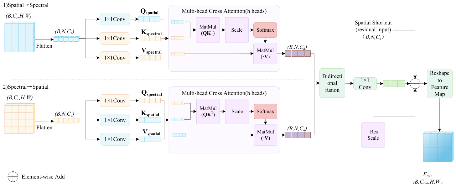
Conventional cross-attention methods usually perform one-way information transfer [32], where one feature domain guides the other domain without reciprocal interaction. Such an asymmetric process limits the exchange of information between spectral and spatial representations. To overcome this limitation, the proposed mechanism adopts two interaction paths, including spatial-to-spectral and spectral-to-spatial paths, so that the two feature domains can provide information for each other.
Furthermore, multi-head attention is employed to model relationships among different feature subspaces. The multiple attention heads allow the module to learn diverse spectral–spatial dependencies. A residual scaling strategy is also adopted to adjust the contribution of cross-domain features and improve the stability of feature fusion during training.
In BSCF-Net, BSCA establishes bidirectional interactions between spectral and spatial representations, enabling spatial structures to refine spectral reconstruction and spectral signatures to guide spatial context modeling.
As illustrated in Figure 2, the bidirectional balanced cross-attention module reshapes the spatial and spectral features into token sequences with H × W spatial positions to facilitate cross-domain interaction. The query, key, and value representations are subsequently obtained through linear projections.
The spatial-guided spectral enhancement process can be formulated as:
F s p = Softmax Q s K p d V p
where Q s is the query projection generated from spatial features, while K p and V p denote the key and value projections derived from spectral features, respectively.
Correspondingly, the spectral-guided spatial compensation process can be formulated as:
F p s = Softmax Q p K s d V s
where Q p is generated from spectral features, and K s and V s are projected from spatial features.
The bidirectional interaction features are subsequently aggregated and used to refine the spatial representation through a learnable residual scaling strategy:
F fusion = F s + α · GELU BN Conv 1 × 1 F s p + F p s
where F s denotes the spatial feature representation used as the residual reference, and α is a learnable residual scaling factor that adjusts the influence of the aggregated bidirectional spectral–spatial interaction features during feature refinement.

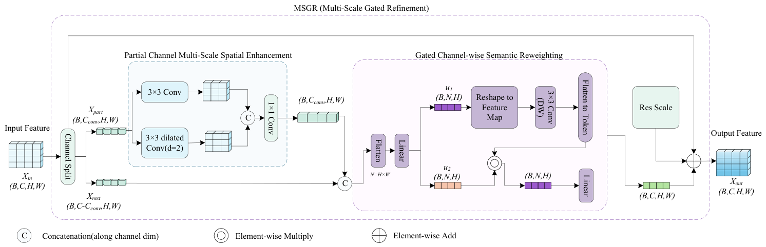
2.3. Multi-Scale Gated Refiner

After obtaining the fused features, a Multi-Scale Gated Refiner is introduced for feature refinement. The module jointly exploits spatial structural information and channel information to perform adaptive feature selection and reconstruction. This process reduces the influence of redundant background information on subsequent reconstruction.
Let the input fused feature generated by the BSCA module be denoted as:
F fusion R B × C × H × W
where B denotes the batch size, C represents the channel dimension, and H and W denote the spatial height and width, respectively.

2.3.1. Partial Channel Multi-Scale Spatial Enhancement Mechanism

Different channels usually contain different levels of spatial information, and not all feature channels require complex spatial modeling operations. Applying spatial modeling to all channels increases computational cost and may introduce redundant information. Therefore, only a portion of the channels is selected for spatial modeling, while the remaining channels retain their original features.
Let the channel partition ratio be denoted as r ( 0 , 1 ] . The fused feature is divided into two parts along the channel dimension:
F fusion = [ F c , F u ] ,
where F c R B × r C × H × W denotes the participating channels for spatial refinement, and F u R B × ( 1 r ) C × H × W represents the channels that retain the original feature information. This channel separation allows the module to perform spatial refinement on selected channels instead of applying additional operations to the entire feature map.
The selected feature channels are further processed by two convolutional branches with different receptive fields. A standard 3 × 3 convolution is used to extract local spatial patterns, while a dilated convolution branch is introduced to enlarge the receptive field and obtain additional contextual information:
F 3 = ϕ Conv 3 × 3 ( F c )
F d i l = ϕ DConv 3 × 3 d = 2 ( F c )
where DConv d = 2 denotes dilated convolution with dilation rate 2.
The multi-scale features are concatenated and fused through a point-wise convolution:
F m = ϕ Conv 1 × 1 ( [ F 3 , F d i l ] )
Finally, the refined channels and untouched channels are concatenated to generate the enhanced spatial representation:
F s r = [ F m , F u ]
The output feature integrates the refined spatial information from selected channels with the original features retained in untouched channels. It provides enhanced spatial representations while introducing only limited computational overhead.

2.3.2. Gated Channel-Wise Semantic Reweighting Mechanism

After spatial enhancement, the extracted features contain spatial information from different receptive fields. However, the contribution of different channels to anomaly representation is not identical, and some channels may still preserve redundant background responses. A gated channel-wise feature re-selection mechanism is designed to adjust channel responses and refine the semantic representation of anomaly-related features.
First, the spatial features are reshaped into a pixel-wise feature sequence:
Z R B × ( H W ) × C
where the spatial dimensions are flattened into a sequence representation while the channel dimension remains unchanged. The reshaped features are further processed by linear projection and channel-wise interaction.
Subsequently, a linear projection is applied to map the features into a higher-dimensional latent space, and the projected features are split along the channel dimension into a feature branch and a gating branch:
[ U 1 , U 2 ] = ϕ ( Z W 1 )
where U 1 , U 2 R B × ( H W ) × C h , C h denotes the hidden feature dimension, and W 1 is a learnable projection matrix.
To introduce local contextual dependencies, a depthwise convolution is applied to U 1 :
U ˜ 1 = DWConv 3 × 3 ( U 1 )
The depthwise convolution is performed separately on each channel to introduce local spatial information with only a small increase in the number of parameters.
Then, an element-wise gating mechanism is employed to perform feature re-selection:
G = U ˜ 1 U 2
where ⊙ denotes element-wise multiplication.
Finally, the refined features are projected back to the original channel dimension via a linear transformation, and a residual connection with learnable scaling is introduced to stabilize training:
F refined = F fusion + β · Reshape ( G W 2 )
where W 2 is a learnable projection matrix, and β denotes a learnable residual scaling factor.
The proposed refiner combines partial-channel spatial enhancement and gated channel-wise reweighting to reduce redundant background information and refine anomaly-related features.

2.3.3. Mechanism Summary

The msGR combines partial-channel spatial enhancement with gated channel selection to refine the fused features and suppress redundant background information.
Figure 3 illustrates the structure of the proposed refinement module. The refined features are subsequently fed into the decoder for progressive reconstruction.

3. Results

3.1. Experimental Datasets

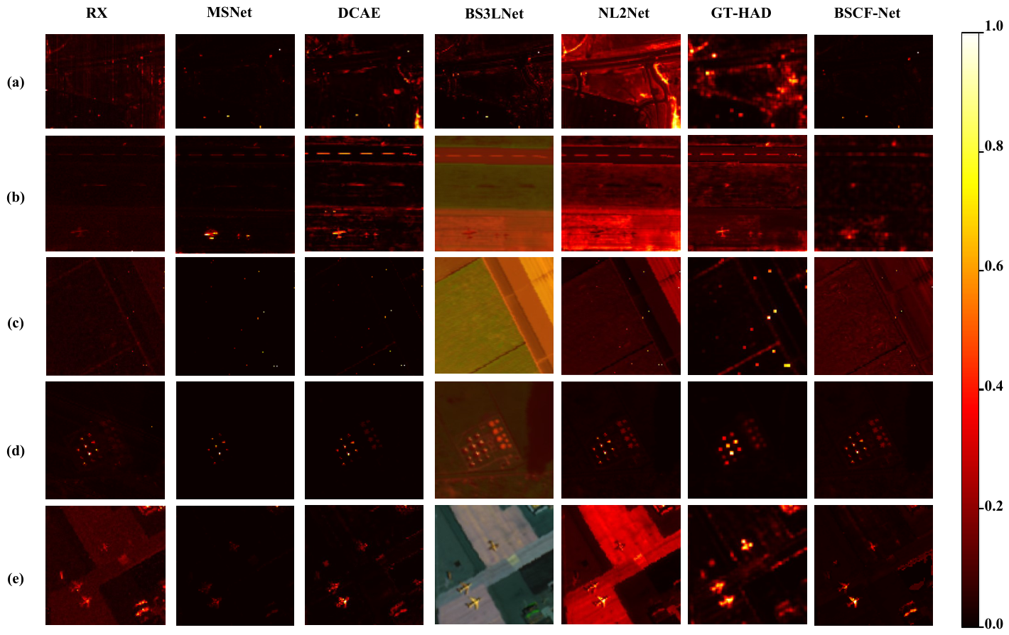
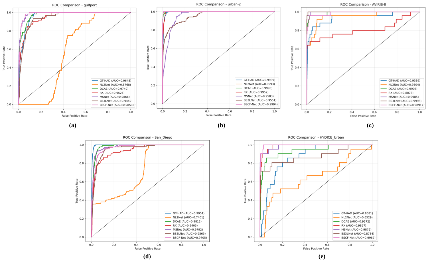
This section presents the anomaly detection results on five datasets. Qualitative evaluation is provided through the anomaly maps in Figure 4, while quantitative evaluation is conducted using ROC curves and AUC values shown in Figure 5 and Table 2. The results for each dataset are discussed below.
HYDICE Urban: This dataset was acquired by the HYDICE sensor and consists of 80 × 100 pixels with 175 spectral bands. It depicts a complex urban scene characterized by diverse background materials and significant spectral variations. The anomalies mainly consist of small artificial objects distributed within cluttered urban areas.
Urban-2: Urban-2 is a widely used hyperspectral anomaly detection dataset with a spatial size of 100 × 100 pixels and 198 spectral bands [33]. The scene contains buildings, roads, vegetation, and shadows, resulting in significant spectral and spatial heterogeneity. The anomalous regions are relatively small and sparsely distributed within the background.
AVIRIS: This dataset was acquired by the AVIRIS sensor and has a spatial resolution of 120 × 120 pixels with 204 spectral bands. It contains relatively regular urban structures and a more homogeneous background. The spectral differences between anomalous regions and their surrounding areas are relatively subtle.
San Diego: The San Diego dataset [34] was collected by the AVIRIS sensor over an airport area in California. It consists of 100 × 100 pixels and contains 189 valid spectral bands after noisy bands were removed. The scene includes runways, aprons, and vegetation. The anomalies are three small aircraft occupying approximately 58 pixels in total.
Gulfport: The Gulfport dataset [35] was acquired by the AVIRIS sensor and consists of 100 × 100 pixels with 191 spectral bands. The scene covers airport facilities and surrounding urban infrastructure. The anomalous targets are relatively large aircraft with clear spatial structures.

3.2. Compared Methods and Experimental Settings

Both traditional and deep learning-based methods [24,36,37] are selected as comparison algorithms. Specifically, the traditional method includes RX, while the deep learning-based methods consist of msNet, DCAE [38], NL2Net [39], GT-HAD [40], and BS3LNet [41]. These methods represent different technical paradigms, including statistical modeling, autoencoder-based reconstruction, Transformer-based feature learning, and self-supervised learning.
Following the common setting of unsupervised hyperspectral anomaly detection, the proposed model is trained separately for each hyperspectral scene without using anomaly labels.
All experiments were implemented using the PyTorch framework with CUDA acceleration. A random seed of 42 was fixed to ensure reproducibility. The proposed model was optimized using the Adam optimizer with an initial learning rate of 1 × 10 2 . The training process was conducted for 500 epochs with a batch size of 1, considering the limited size of hyperspectral datasets. The mean squared error (MSE) between the input image and reconstructed image was adopted as the reconstruction loss.
The input hyperspectral data were projected into a 64-dimensional latent space for subsequent feature extraction. In the spectral branch, a one-dimensional convolution with a kernel size of 3 was employed to extract spectral representations. In the spatial branches, a 7 × 7 depthwise separable convolution and a 3 × 3 convolution were utilized to capture large-scale and local spatial patterns, respectively. The BSCA module employed four attention heads, and the residual scaling factor was initialized to 0.1. For the msGR module, the partial ratio, dilation rate, and hidden dimension were set to 0.5, 2, and 128, respectively.
During inference, the anomaly score of each pixel was calculated based on the spectral reconstruction residual between the input hyperspectral image X and the reconstructed image X ^ . Specifically, the anomaly score is defined as:
S ( i , j ) = 1 B b = 1 B ( X b ( i , j ) X ^ b ( i , j ) ) 2 ,
where B denotes the number of spectral bands. A larger value of S ( i , j ) indicates a larger reconstruction discrepancy and a higher probability of being an anomaly. The generated anomaly score maps were evaluated using the receiver operating characteristic (ROC) curve and the area under the curve (AUC).
The experiments were conducted using PyTorch 2.4.1 on a Linux server equipped with an NVIDIA RTX 4090 GPU. The traditional RX method was executed on the same platform using PyCharm for fair comparison. The implementation details of DCAE, NL2Net, BS3LNet, GT-HAD, and msNet followed their original papers.

3.3. Experimental Results

The anomaly detection results of different methods on the five datasets are presented in this section. Figure 4 displays the anomaly maps produced by different methods, and Figure 6 shows the response distributions of background and anomaly pixels using box plots. The ROC curves and AUC values are given in Figure 5 and Table 2, respectively [42]. The results obtained on each dataset are discussed in the following parts.
Anomaly Maps: Figure 4 presents the anomaly detection maps produced by different methods on the five datasets. Overall, BSCF-Net effectively suppresses background responses while highlighting anomalous regions.
Specifically, RX, msNet, and DCAE can suppress background responses to a certain extent. However, in complex urban scenes such as HYDICE Urban and Gulfport, their responses to some anomalous targets are relatively weak, resulting in unclear target boundaries. BS3LNet and NL2Net are more susceptible to background interference on datasets such as AVIRIS and San Diego, producing a considerable number of high-response regions in the detection maps. GT-HAD can effectively highlight anomalous targets, but its detection results exhibit noticeable block-like artifacts.In contrast, BSCF-Net maintains low background responses across all five datasets while effectively highlighting anomalous regions. In complex scenes such as Urban-2 and San Diego, the proposed method still produces clear anomaly responses. These results demonstrate that BSCF-Net achieves superior performance in both background suppression and anomaly detection.
To further analyze the performance differences among various methods, a detailed comparison on each dataset is discussed as follows.
Table 2 reports the AUC results of different methods on five hyperspectral datasets. BSCF-Net achieves superior performance on most datasets and shows stable results under different background conditions.
The results in the table show that BSCF-Net obtained the highest AUC values on the Gulfport, HYDICE Urban, and Urban-2 datasets, with values of 0.9866, 0.9962, and 0.9994, respectively.
The performance of several comparison methods was lower on the Gulfport dataset. For example, NL2Net achieved an AUC of 0.5768, whereas BSCF-Net reached 0.9866. On the HYDICE Urban dataset, BSCF-Net also achieved the best result among all compared methods. Although most methods obtained high AUC values on the Urban-2 dataset, BSCF-Net still showed better performance. On the AVIRIS and San Diego datasets, BSCF-Net did not rank first, but the difference from the best-performing method was relatively small.
Overall, BSCF-Net showed consistent detection performance across the evaluated datasets.
To evaluate the training stability, multiple independent runs were conducted for deep-learning methods with similar network architectures and compositions, including DCAE, NL2Net, BS3LNet, and BSCF-Net.
To further evaluate the training stability of the compared deep-learning methods, five independent runs were conducted on each dataset. The mean and standard deviation of the AUC are reported in Table 3. BSCF-Net obtains the highest mean AUC on all five datasets, with values of 0.9883, 0.9842, 0.9952, 0.9994, and 0.9692 on AVIRIS, Gulfport, HYDICE Urban, Urban-2, and San Diego, respectively. These results show that BSCF-Net performs well under different background conditions.
BSCF-Net also shows relatively small standard deviations on AVIRIS (0.0064), HYDICE Urban (0.0016), Urban-2 (0.0001), and San Diego (0.0073). The standard deviation on Urban-2 is only 0.0001, indicating highly consistent results across the five runs. A larger variation is observed on Gulfport, where the standard deviation reaches 0.0223. This indicates that the results on this dataset are more sensitive to the training process. The complex background and the difficulty of distinguishing anomalous targets from background pixels may contribute to this variation. On the Gulfport dataset, the mean AUC of BSCF-Net is still 0.9842, which is higher than those of DCAE (0.9792), NL2Net (0.5775), and BS3LNet (0.9462). Overall, BSCF-Net provides competitive detection accuracy and shows relatively stable performance across the independent training runs.
Anomaly Detection Accuracy: Figure 5 presents the ROC curves and corresponding AUC values of different methods on the five datasets. A ROC curve closer to the upper-left corner indicates better detection performance and corresponds to a higher AUC value, suggesting that the detection result is closer to the ideal case.
As shown in Figure 5, RX relies on the assumption that background information can be described by a global statistical model. Therefore, its detection performance may decrease when the background distribution becomes more complex. For example, on datasets such as HYDICE Urban, the ROC curve of RX deviates noticeably from the upper-left corner, resulting in relatively limited detection performance.
Some deep learning-based methods, such as NL2Net and DCAE, achieve relatively good results on certain datasets. However, their performance varies under different background conditions. For instance, NL2Net suffers from a clear performance degradation on the San Diego dataset, indicating that its feature representation is affected by complex spatial structures and background variations.
In comparison, BSCF-Net maintains stable ROC performance across all evaluated datasets, with the curves generally remaining closer to the upper-left corner. The spectral–spatial feature interaction and refinement process help the network obtain more consistent anomaly representations under different scene conditions. In the low false positive rate region, BSCF-Net shows a faster increase in the true positive rate, allowing more anomalous pixels to be detected while keeping false alarms at a relatively low level.
From the perspective of AUC, BSCF-Net achieves the best or near-best performance on multiple datasets. In particular, it obtains an AUC value of 0.9962 on the HYDICE Urban dataset, which indicates that the proposed method can better handle scenes with complex background distributions. These results demonstrate that BSCF-Net provides stable detection performance across different hyperspectral datasets.
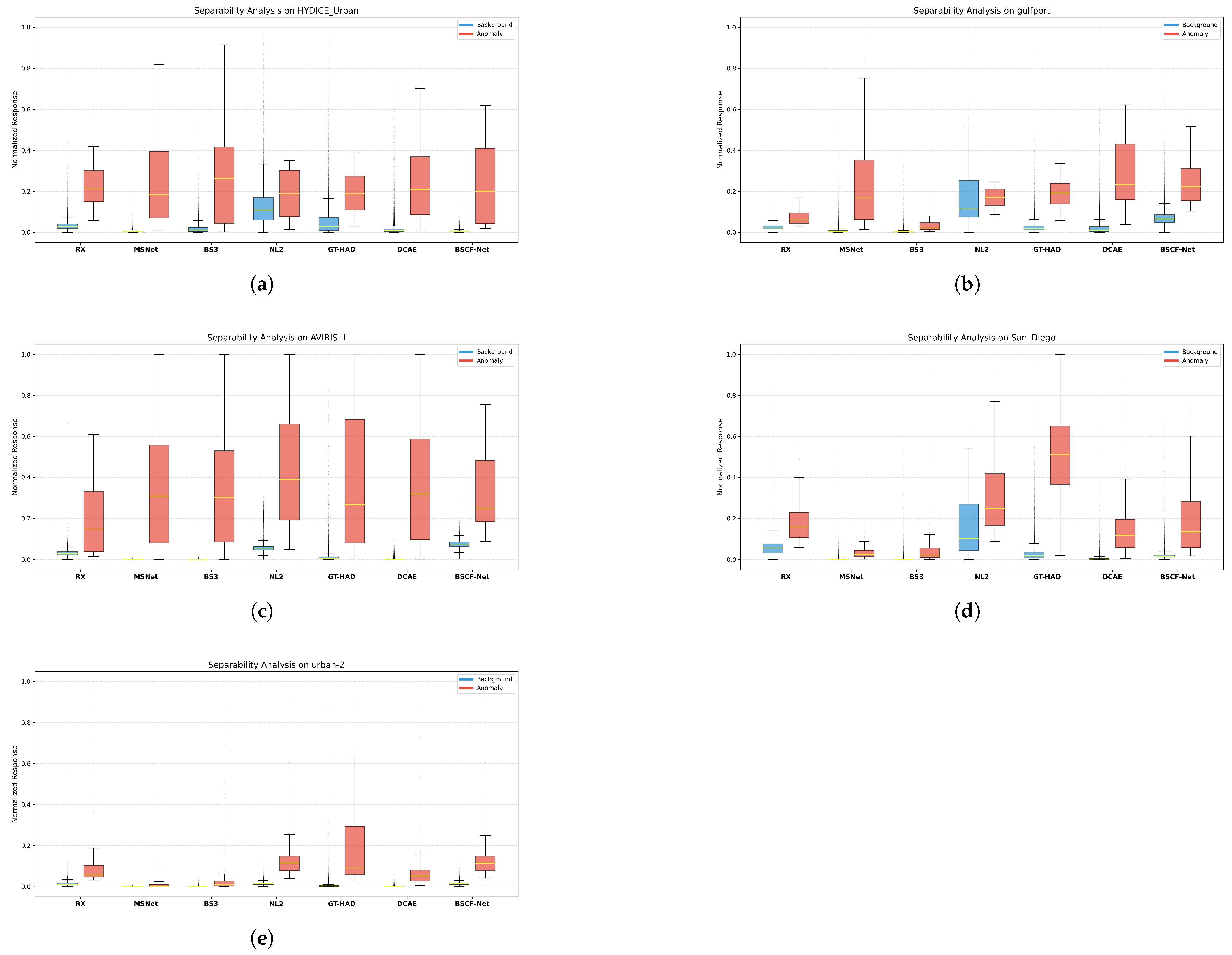
Separation of Background and Anomalies: Figure 6 shows box plots of detection response distributions for different methods on the five datasets. The separability between background and anomaly responses reflects the discriminative capability of each method. Background responses (blue boxes) are typically concentrated in lower value ranges, while anomaly responses (orange boxes) are distributed in higher value regions. A smaller overlap between the two distributions indicates better separation.
Across the five datasets, different methods exhibit distinct distributions of background and anomaly responses. RX, msNet, and BS3 produce relatively low anomaly responses in most datasets, with noticeable overlap between background and anomaly distributions. NL2Net achieves higher anomaly responses on some datasets, but its performance varies across different scenarios. GT-HAD and DCAE generally yield higher anomaly responses, although their background responses still show certain variations.
In contrast, BSCF-Net exhibits stable distribution characteristics across all datasets. The background responses are consistently lower and more concentrated, while the anomaly responses are higher, resulting in a clear separation between the two distributions. This separation is more pronounced in the Urban-2 and HYDICE Urban datasets. In the Gulfport and San Diego datasets, the overlap between background and anomaly distributions is relatively small.
From the results, it can be observed that different methods show varying separability across datasets, whereas BSCF-Net maintains a consistent distribution structure across multiple scenarios.

3.4. Ablation Study

To evaluate the effectiveness of each component in BSCF-Net, ablation studies are conducted by separately removing the refinement module and the bidirectional fusion module, while keeping all other network structures and training settings unchanged. The results are reported in Table 4.
As shown in the observations, both modules contribute to the overall detection performance, with the bidirectional fusion module having a more pronounced effect. The refinement module primarily improves detection performance by suppressing residual background noise and enhancing anomaly responses. On datasets with relatively clear structures, such as HYDICE Urban and Urban-2, removing this module results in only a slight performance drop; however, on datasets with more complex background distributions, such as Gulfport and San Diego, the performance degradation becomes more pronounced.After removing the bidirectional fusion module, the detection performance drops significantly across most datasets, particularly on the Gulfport and HYDICE Urban datasets, where the AUC decreases to 0.5511 and 0.6679, respectively, indicating a substantial decline.
The results indicate that the bidirectional fusion module plays a primary role in cross-domain feature interaction, while the refinement module is mainly responsible for improving feature quality. The combination of both modules enables the model to maintain relatively stable detection performance across different datasets.

3.5. Computational Complexity Analysis

As shown in Table 5, the computational cost of BSCF-Net varies slightly among the five hyperspectral datasets, mainly due to the differences in input spatial and spectral dimensions. The number of parameters ranges from 0.3499 M to 0.3611 M, with an average value of 0.3562 M. Although BSCF-Net introduces additional parameters compared with some lightweight anomaly detection networks, the overall model size remains relatively compact. This increase mainly results from the incorporation of multiscale convolution operations and bidirectional spectral–spatial cross-attention, which are designed to enhance the representation capability of complex spectral–spatial patterns.
In terms of computational operations, BSCF-Net requires 5.5230–10.2622 G FLOPs across the five datasets, with an average computational cost of 7.3807 G FLOPs. Compared with conventional reconstruction-based methods, the proposed network has a higher computational burden due to the additional feature interaction and refinement processes. Specifically, the bidirectional spectral–spatial cross-attention module introduces extra computational overhead for spectral–spatial feature alignment, while the multiscale spatial branches increase the receptive field modeling capability through multiple convolution operations. However, these additional computations enable BSCF-Net to capture complementary information from different spectral and spatial scales, which contributes to improved anomaly detection performance in complex hyperspectral scenes.
The AVIRIS dataset requires the highest computational cost, reaching 10.2622 G FLOPs and 48.1710 ms/image inference time, mainly because of its larger spatial and spectral dimensions. In contrast, the Urban-2 dataset requires only 5.5230 G FLOPs and 15.4207 ms/image due to its relatively smaller input size. The average inference time of BSCF-Net is 26.8914 ms per hyperspectral image on the NVIDIA RTX 4090 GPU. Although the proposed model introduces higher computational complexity than some existing methods, the additional cost remains acceptable considering the significant improvement in spectral–spatial feature representation. These results demonstrate that BSCF-Net achieves a favorable trade-off between detection accuracy and computational efficiency.

4. Discussion

Experimental results show that Spectral–Spatial interaction plays an important role in hyperspectral anomaly detection, especially in scenes containing small targets and complex backgrounds. Spectral information mainly reflects the material characteristics of targets, whereas spatial information describes their structural and contextual properties. Combining these two types of information helps improve anomaly representation under complex background conditions. The bidirectional interaction mechanism enhances information exchange between spectral and spatial domains and produces more consistent and discriminative feature representations. Different from one-way feature interaction, this strategy allows both domains to contribute to feature enhancement and alleviates the limitation of separately modeling spectral and spatial features.
The multiscale refinement module further enhances local anomaly responses by refining the fused features from different spatial scales. At the same time, it removes part of the redundant background information in the feature representation. Therefore, anomaly regions can be represented more clearly, while false alarms caused by background interference can be reduced. The ablation results indicate that the refinement module benefits from the features generated by the fusion module, and the two modules show a complementary relationship in anomaly detection. The fusion features provide a basis for subsequent refinement, and the refinement process further adjusts the feature responses related to anomalies.
Although BSCF-Net performs well on several public datasets, the use of multiscale convolutions and bidirectional attention mechanisms introduces additional computational cost. BSCF-Net achieves improved detection performance at the cost of additional computational complexity. This complexity mainly results from multi-scale feature extraction and cross-domain feature interaction. Future work will focus on lightweight network designs to reduce computational requirements while preserving detection accuracy. Improving model robustness under low signal-to-noise ratio conditions will also be considered in future studies.
BSCF-Net does not achieve the highest AUC on every dataset, indicating that the performance of anomaly detection methods may vary under different scene characteristics. Different datasets contain different background distributions and anomaly patterns, which may affect the effectiveness of feature extraction and reconstruction. Therefore, the performance differences among methods are related to the specific characteristics of each scene.
Although several recent HAD methods have been included for comparison, some methods such as DeCNN-AD [43] were not evaluated due to the lack of a complete reproducible implementation. The publicly available code requires additional MATLAB R2023b dependencies and missing configuration files, making it difficult to establish a fair comparison under our experimental environment.

5. Conclusions

This paper presents BSCF-Net for hyperspectral anomaly detection, aiming to improve the interaction between spectral and spatial features and enhance multi-scale feature representation. The proposed network integrates bidirectional cross-domain fusion with multi-scale refinement to extract more discriminative feature representations and reduce the interference caused by complex backgrounds. By enabling information exchange between spectral and spatial domains, the network better utilizes the complementary characteristics of different feature types.
Experiments conducted on several public hyperspectral datasets demonstrate that BSCF-Net achieves competitive detection performance compared with existing methods. The proposed method maintains stable detection results under different background conditions and shows advantages in scenes containing small targets and complex spatial structures. These results indicate that the combination of spectral–spatial interaction and feature refinement is beneficial for improving hyperspectral anomaly detection performance.

Author Contributions

Conceptualization, Y.G. and M.W.; methodology, M.W. and Y.G.; software, M.W.; validation, M.W.; data curation, M.W.; investigation, M.W.; formal analysis, M.W. and Y.G.; writing—original draft preparation, M.W.; writing—review and editing, Y.G., L.Z., T.Y., H.W. and W.Z.; supervision, Y.G.; project administration, Y.G., T.Y., H.W. and W.Z. All authors have read and agreed to the published version of the manuscript.

Funding

This research was funded by the National Natural Science Foundation of China under Grant No. 62106195.

Institutional Review Board Statement

Not applicable.

Informed Consent Statement

Not applicable.

Data Availability Statement

The datasets used in this study are publicly available and can be obtained from publicly accessible repositories and related publications.

Acknowledgments

During the preparation of this manuscript, the authors used [GPT-5.5-mini] for the purposes of grammar correction, language polishing, and translating a portion of the text. The authors have reviewed and edited the output and take full responsibility for the content of this publication.

Conflicts of Interest

The authors declare no conflicts of interest.

References

  1. Yu, L.; Liu, Y.; Gao, H. Blind-Spot KAN-Based Background Reconstruction Network with Prior Purification for Hyperspectral Anomaly Detection. Remote Sens. 2026, 18, 1628. [Google Scholar] [CrossRef] [Scilit]
  2. Reed, I.S.; Yu, X. Adaptive multiple-band CFAR detection of an optical pattern with unknown spectral distribution. IEEE Trans. Acoust. Speech Signal Process. 1990, 38, 1760–1770. [Google Scholar] [CrossRef] [Scilit]
  3. Garske, S.; Evans, B.; Artlett, C.; Wong, K.C. ERX: A fast real-time anomaly detection algorithm for hyperspectral line scanning. IEEE Trans. Geosci. Remote Sens. 2025, 63, 5503617. [Google Scholar] [CrossRef] [Scilit]
  4. Liu, W.-M.; Chang, C.-I. Multiple-window anomaly detection. IEEE J. Sel. Top. Appl. Earth Obs. Remote Sens. 2013, 6, 644–658. [Google Scholar] [CrossRef] [Scilit]
  5. Guo, Q.; Zhang, B.; Ran, Q.; Gao, L.; Li, J.; Plaza, A. Weighted-RXD anomaly detection. IEEE J. Sel. Top. Appl. Earth Obs. Remote Sens. 2014, 7, 2351–2366. [Google Scholar] [CrossRef] [Scilit]
  6. Ma, X.; Zhang, X.; Tang, X.; Zhou, H.; Jiao, L. Hyperspectral Anomaly Detection Based on Low-Rank Representation With Data-Driven Projection and Dictionary Construction. IEEE J. Sel. Top. Appl. Earth Obs. Remote Sens. 2020, 13, 2226–2239. [Google Scholar] [CrossRef] [Scilit]
  7. Chang, C.-I.; Cao, H.; Chen, S.; Shang, X.; Yu, C.; Song, M. Orthogonal subspace projection-based Go-decomposition approach for hyperspectral anomaly detection. IEEE Trans. Geosci. Remote Sens. 2021, 59, 2403–2429. [Google Scholar] [CrossRef] [Scilit]
  8. Li, F.; Zhang, Y.; Zhang, L.; Zhang, X.; Jiang, D. Hyperspectral anomaly detection using background learning and structured sparse representation. In Proceedings of the 2016 IEEE International Geoscience and Remote Sensing Symposium (IGARSS), Beijing, China, 10–15 July 2016; pp. 1618–1621. [Google Scholar]
  9. Xu, Y.; Du, B.; Zhang, L.; Chang, S. Low-rank and sparse matrix decomposition-based anomaly detection. IEEE Geosci. Remote Sens. Lett. 2020, 17, 1248–1252. [Google Scholar] [CrossRef] [Scilit]
  10. Li, S.; Wang, W.; Qi, H.; Ayhan, B.; Kwan, C.; Vance, S. Low-rank tensor decomposition-based anomaly detection. In Proceedings of the 2015 IEEE International Conference on Image Processing (ICIP), Quebec City, QC, Canada, 27–30 September 2015; pp. 4525–4529. [Google Scholar]
  11. Lin, S.; Cheng, X.; Zeng, Y.; Huo, Y.; Zhang, M.; Wang, H. Low-rank and sparse representation inspired interpretable network for hyperspectral anomaly detection. IEEE Trans. Instrum. Meas. 2024, 73, 5033116. [Google Scholar] [CrossRef] [Scilit]
  12. Li, W.; Du, Q. Collaborative representation for anomaly detection. IEEE Trans. Geosci. Remote Sens. 2015, 53, 1463–1474. [Google Scholar] [CrossRef] [Scilit]
  13. Wang, M.; Wang, Q.; Hong, D.; Roy, S.K.; Chanussot, J. Tensor low-rank representation. IEEE Trans. Cybern. 2023, 53, 679–691. [Google Scholar] [CrossRef] [Scilit] [PubMed]
  14. Yang, X.; Wei, Y.; Tan, J.; Li, S.; Tang, H.; Liu, W. LMamba: Local-Guided Mamba with Multi-Scale Filtering for Hyperspectral Image Classification. Remote Sens. 2026, 18, 1629. [Google Scholar] [CrossRef] [Scilit]
  15. Li, Y.-X.; Yeh, H.-Y. A semi-supervised learning model based on convolutional autoencoder and convolutional neural network for image classification. In Proceedings of the 2019 International Symposium on Intelligent Signal Processing and Communication Systems (ISPACS), Taipei, Taiwan, 3–6 December 2019. [Google Scholar]
  16. Chen, Y.; Zhang, H.; Wang, Y.; Wu, Q.M.J.; Yang, Y. Projected sliced Wasserstein autoencoder for hyperspectral anomaly detection. arXiv 2021, arXiv:2112.11243. [Google Scholar]
  17. Lv, S.; Zhao, S.; Li, D.; Pang, B.; Lian, X.; Liu, Y. Spatial–spectral joint hyperspectral anomaly detection. Remote Sens. 2023, 15, 2542. [Google Scholar] [CrossRef] [Scilit]
  18. Yu, D.; Gao, Z. VolFormer: Explore more comprehensive cube interaction for hyperspectral image restoration and beyond. In Proceedings of the 2025 IEEE/CVF Conference on Computer Vision and Pattern Recognition (CVPR), Nashville, TN, USA, 10–17 June 2025; pp. 28091–28101. [Google Scholar]
  19. Park, J.; Woo, S.; Lee, J.-Y.; Kweon, I.S. BAM: Bottleneck attention module. arXiv 2018, arXiv:1807.06514. [Google Scholar]
  20. Woo, S.; Park, J.; Lee, J.-Y.; Kweon, I.S. CBAM: Convolutional block attention module. In Computer Vision—ECCV 2018; Springer: Berlin/Heidelberg, Germany, 2018; pp. 3–19. [Google Scholar]
  21. Chong, D.; Hu, B.; Gao, H.; Gao, X. Hyperspectral anomaly detection via super-resolution reconstruction. Appl. Opt. 2021, 60, 8109–8119. [Google Scholar] [CrossRef] [Scilit] [PubMed]
  22. Wang, D.; Ren, L.; Sun, X.; Gao, L.; Chanussot, J. Nonlocal and local feature-coupled self-supervised network for hyperspectral anomaly detection. IEEE J. Sel. Top. Appl. Earth Obs. Remote Sens. 2025, 18, 6981–6993. [Google Scholar] [CrossRef] [Scilit]
  23. Zhang, G.; Sun, T.; Lu, F.; Zhang, S.; Yin, J.; Wu, Y.; Xiong, Z. FS2CCTrans: Frequency–spatial–spectral joint analysis with criss-cross transformer for hyperspectral anomaly detection. IEEE Trans. Geosci. Remote Sens. 2025, 63, 5508218. [Google Scholar] [CrossRef] [Scilit]
  24. Gan, Y.; Li, X.; Wu, S.; Wang, M. MACNet: A multiscale attention guided contextual network for hyperspectral anomaly detection. IEEE Geosci. Remote Sens. Lett. 2025, 22, 5508905. [Google Scholar] [CrossRef] [Scilit]
  25. Ren, X.; Wang, J.; Ma, T.; Yue, C.; Bai, K. Adaptive background suppression method for IR small target detection. IEEE Access 2020, 8, 36930–36947. [Google Scholar] [CrossRef] [Scilit]
  26. Wang, Y.; Mu, Z.; Zhang, H.; Song, C.; Wang, X. Robust Hyperspectral Anomaly Detection via Unsupervised Multiscale Feature Fusion. Remote Sens. 2026, 18, 1554. [Google Scholar] [CrossRef] [Scilit]
  27. Wang, M.; Yang, K.; Lu, J.; Liu, W.; Zeng, T. A Spectral Variability and Class-Constrained Diffusion Model for Unsupervised Hyperspectral Unmixing. Remote Sens. 2026, 18, 1483. [Google Scholar] [CrossRef] [Scilit]
  28. Zhou, S.; Chen, D.; Pan, J.; Shi, J.; Yang, J. Adapt or perish: Adaptive sparse transformer with attentive feature refinement for image restoration. In Proceedings of the 2024 IEEE/CVF Conference on Computer Vision and Pattern Recognition (CVPR), Seattle, WA, USA, 16–22 June 2024; pp. 2952–2963. [Google Scholar]
  29. Wang, A.; Chen, H.; Lin, Z.; Han, J.; Ding, G. LSNet: See large, focus small. In Proceedings of the 2025 IEEE/CVF Conference on Computer Vision and Pattern Recognition (CVPR), Nashville, TN, USA, 10–17 June 2025; pp. 9718–9729. [Google Scholar]
  30. Howard, A.G.; Zhu, M.; Chen, B.; Kalenichenko, D.; Wang, W.; Weyand, T.; Andreetto, M.; Adam, H. MobileNets: Efficient Convolutional Neural Networks for Mobile Vision Applications. arXiv 2017, arXiv:1704.04861. [Google Scholar]
  31. Wang, J.; Wu, Z.; Ouyang, W.; Han, X.; Chen, J.; Lim, S.-N.; Jiang, Y.-G. M2TR: Multi-modal multi-scale transformers for deepfake detection. In Proceedings of the 2022 International Conference on Multimedia Retrieval, Newark, NJ, USA, 27–30 June 2022; pp. 615–623. [Google Scholar]
  32. Vaswani, A.; Shazeer, N.; Parmar, N.; Uszkoreit, J.; Jones, L.; Gomez, A.N.; Kaiser, Ł.; Polosukhin, I. Attention is all you need. In Proceedings of the Advances in Neural Information Processing Systems NIPS, Long Beach, CA, USA, 4–9 December 2017; pp. 5998–6008. [Google Scholar]
  33. Liu, S.; Zhu, C.; Ran, D.; Wen, G. Tensor multisubspace learning for anomaly detection. IEEE J. Sel. Top. Appl. Earth Obs. Remote Sens. 2023, 16, 8178–8190. [Google Scholar] [CrossRef] [Scilit]
  34. Green, R.O.; Eastwood, M.L.; Sarture, C.M.; Chrien, T.G.; Aronsson, M.; Chippendale, B.J.; Faust, J.A.; Pavri, B.E.; Chovit, C.J.; Solis, M.; et al. Imaging Spectroscopy and the Airborne Visible/Infrared Imaging Spectrometer (AVIRIS). Remote Sens. Environ. 1998, 65, 227–248. [Google Scholar] [CrossRef] [Scilit]
  35. Kang, X.; Zhang, X.; Li, S.; Li, K.; Li, J.; Benediktsson, J.A. Hyperspectral Anomaly Detection with Attribute and Edge–Preserving Filters. IEEE Trans. Geosci. Remote Sens. 2017, 55, 5600–5611. [Google Scholar] [CrossRef] [Scilit]
  36. Wu, Z.; Wang, B. KACNet: Kolmogorov–Arnold convolution network for Hyperspectral Anomaly Detection. IEEE Trans. Geosci. Remote Sens. 2025, 63, 5506514. [Google Scholar] [CrossRef] [Scilit]
  37. Fu, X.; Zhang, T.; Cheng, J.; Jia, S. MMR-HAD: Multiscale Mamba reconstruction network. IEEE Trans. Geosci. Remote Sens. 2025, 63, 5516914. [Google Scholar] [CrossRef] [Scilit]
  38. Wu, Z.; Paoletti, M.E.; Su, H.; Tao, X.; Han, L.; Haut, J.M.; Plaza, A. Background-guided deformable convolutional autoencoder for hyperspectral anomaly detection. IEEE Trans. Geosci. Remote Sens. 2023, 61, 5531816. [Google Scholar] [CrossRef] [Scilit]
  39. Wu, Z.; Wang, B. Transformer-Based Autoencoder Framework for Nonlinear Hyperspectral Anomaly Detection. IEEE Trans. Geosci. Remote Sens. 2024, 62, 5508015. [Google Scholar] [CrossRef] [Scilit]
  40. Lian, J.; Wang, L.; Sun, H.; Huang, H. GT-HAD: Gated transformer for hyperspectral anomaly detection. IEEE Trans. Neural Netw. Learn. Syst. 2025, 36, 3631–3645. [Google Scholar] [CrossRef] [Scilit] [PubMed]
  41. Gao, L.; Wang, D.; Zhuang, L.; Sun, X.; Huang, M.; Plaza, A. BS3LNet: A new blind-spot self-supervised learning network for hyperspectral anomaly detection. IEEE Trans. Geosci. Remote Sens. 2023, 61, 3246565. [Google Scholar] [CrossRef] [Scilit]
  42. Chang, C.-I.; Lin, C.-Y.; Chung, P.-C.; Hu, P.F. Iterative spectral–Spatial hyperspectral anomaly detection. IEEE Trans. Geosci. Remote Sens. 2023, 61, 5504330. [Google Scholar] [CrossRef] [Scilit]
  43. Fu, X.; Jia, S.; Zhuang, L.; Xu, M.; Zhou, J.; Li, Q. Hyperspectral Anomaly Detection via Deep Plug-and-Play Denoising CNN Regularization. IEEE Trans. Geosci. Remote Sens. 2021, 59, 9553–9568. [Google Scholar] [CrossRef] [Scilit]
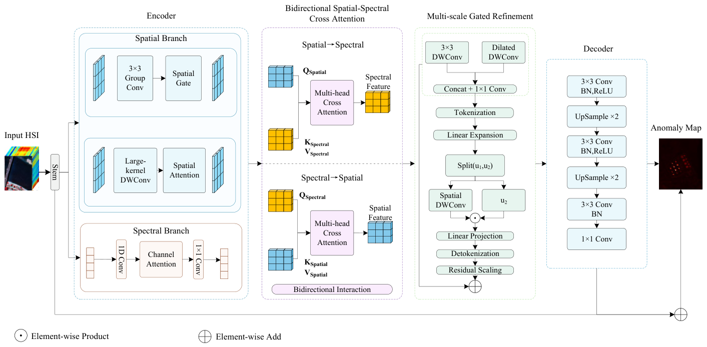
Figure 1. The overall network architecture.
Remotesensing 18 02820 g001
Figure 2. Architecture of the Bidirectional Spectral–Spatial Cross-Attention module.
Remotesensing 18 02820 g002
Figure 3. Architecture of the proposed Multi-Scale Gated Refiner.
Remotesensing 18 02820 g003
Figure 4. Anomaly detection maps on five datasets. (a) HYDICE Urban; (b) Gulfport; (c) AVIRIS; (d) Urban-2; (e) San Diego.
Remotesensing 18 02820 g004
Figure 5. Comparison of ROC Curve Results for Anomaly Detection Across Five Datasets. (a) Gulfport; (b) Urban-2; (c) AVIRIS; (d) San Diego; (e) HYDICE Urban.
Remotesensing 18 02820 g005
Figure 6. Separability between background and anomalies on five datasets. (a) HYDICE Urban, (b) Gulfport, (c) AVIRIS, (d) San Diego, (e) Urban-2.
Remotesensing 18 02820 g006
Table 1. Notation used in this paper.
NotationDescription
X Input hyperspectral feature representation
X s Spatial feature embedding after 1 × 1 convolution
X p Spectral sequence representation of input features
F s Spatial feature representation
F p ( 0 ) Initial spectral features after 1D convolution
F p ( 1 ) Channel-refined spectral features
F p Final spectral feature representation after reshaping
A s Global spatial response map generated by large-kernel branch
M s Local spatial attention map
F l Local spatial features extracted by grouped convolution
F ^ l Local spatial features refined by spatial attention
F s p Spatial-guided spectral enhancement feature
F p s Spectral-guided spatial compensation feature
F f u s i o n Feature representation after BSCA fusion
α Learnable residual scaling factor in BSCA
F c Selected channel group for spatial enhancement in msGR
F u Untouched channel group retaining original features
rChannel partition ratio in partial-channel enhancement
F 3 Features extracted by the local 3 × 3 convolution branch in msGR
F d i l Features extracted by 3 × 3 dilated convolution with dilation rate 2
F m Multi-scale spatial features after feature fusion
F s r Enhanced spatial representation after channel reconstruction
Z Flattened pixel-wise feature sequence
U 1 , U 2 Feature branch and gating branch after channel split
U ˜ 1 Depthwise convolution enhanced feature branch
G Gated feature representation
F r e f i n e d Final refined feature representation from msGR
β Learnable residual scaling factor in msGR
W 1 Weight matrix of the first linear layer in the MLP
W 2 Weight matrix of the second linear layer in the MLP
b 1 Bias vector of the first linear layer
b 2 Bias vector of the second linear layer
Table 2. AUC comparison of different methods on five hyperspectral datasets with a fixed random seed of 42. Bold and underlined values denote the best and second-best results, respectively.
DatasetRXMSNetDCAENL2NetGT-HADBS3LNetBSCF-Net
AVIRIS0.80730.98630.98990.95030.93890.99970.9891
Gulfport0.95260.98530.97400.57680.96480.94590.9866
HYDICE Urban0.98570.97590.89730.65290.86810.87840.9962
Urban-20.99520.96710.99920.99930.99390.95650.9994
San Diego0.94030.96760.89710.74010.97550.95490.9705
Table 3. AUC mean and standard deviation of DCAE, NL2Net, BS3LNet, and BSCF-Net from five independent runs across five hyperspectral datasets. The results are reported as mean ± standard deviation.
DatasetDCAENL2NetBS3LNetBSCF-Net
AVIRIS0.9838 ± 0.01060.9501 ± 0.00480.9996 ± 0.00020.9883 ± 0.0064
Gulfport0.9792 ± 0.00820.5775 ± 0.01260.9462 ± 0.00510.9842 ± 0.0223
HYDICE Urban0.9081 ± 0.00400.6534 ± 0.01870.8791 ± 0.01280.9952 ± 0.0016
Urban-20.9993 ± 0.00020.9993 ± 0.00020.9568 ± 0.00870.9994 ± 0.0001
San Diego0.8962 ± 0.00550.7412 ± 0.01540.9552 ± 0.00630.9692 ± 0.0073
Table 4. Ablation study of key components in BSCF-Net (AUC).
DatasetFull Modelw/o msGRw/o BSCA
HYDICE Urban0.99620.97010.7681
Urban-20.99940.98620.9740
San Diego0.97050.95430.7132
AVIRIS0.98910.97970.9488
gulfport0.99170.90720.7001
Table 5. Computational complexity of BSCF-Net on five hyperspectral datasets.
DatasetParams (M)FLOPs (G)Inference Time (ms/Image)
AVIRIS0.361110.262248.1710
Gulfport0.35617.026723.3947
San Diego0.35537.011323.9320
HYDICE Urban0.34995.523015.4207
Urban-20.35887.080423.5384
Average0.35627.380726.8914
Disclaimer/Publisher’s Note: The statements, opinions and data contained in all publications are solely those of the individual author(s) and contributor(s) and not of MDPI and/or the editor(s). MDPI and/or the editor(s) disclaim responsibility for any injury to people or property resulting from any ideas, methods, instructions or products referred to in the content.