Hyper-VMIL: Topology-Aware Variational Hypergraph Multiple-Instance Learning for Weakly Supervised Hyperspectral Target Detection

Highlights

What are the main findings?

• A topology-conditioned variational inference framework (Hyper-VMIL) resolves bag-level label ambiguity by coupling high-order spatial–spectral hypergraphs with Bernoulli posterior variance regularization derived from the variational ELBO.
• Continuous posterior refinement (CTPR) over the probability simplex avoids the confirmation bias of hard pseudo-labeling, smoothly recovering occluded subpixel targets and achieving superior operational accuracy (${\mathrm{NAUC}}_{\mathrm{FPR}\le {10}^{-3}}=0.577$).
• Confidence-weighted topological knowledge distillation successfully internalizes high-order contextual manifold constraints into a lightweight single-spectrum student network, retaining 96.4% of the contextual teacher’s detection capability.

What are the implications of the main findings?

• A rigorous generative variational foundation for weakly supervised hyperspectral detection is established, preventing error propagation and posterior drift under weak bag-level supervision.
• The gap between high-order topological modeling and real-time onboard remote sensing is bridged, enabling microsecond-level streaming line-scan detection without test-time graph construction.

Abstract

Region-level weakly supervised hyperspectral target detection (HTD) using multiple-instance learning (MIL) reduces annotation costs but encounters challenges such as bag label ambiguity, boundary over-smoothing, and test-time computational latency. To address these issues, we propose Hyper-VMIL, a spatial–spectral topology-regularized variational hypergraph network. Hyper-VMIL formulates latent target localization as variational inference over dual-path hypergraphs: a boundary-aware spatial hypergraph modeling geometric patch continuity and a dynamic spectral-manifold hypergraph capturing non-local material similarity. Node-adaptive gating dynamically balances spatial and spectral evidence to mitigate over-smoothing near target boundaries. Furthermore, a confidence-aware continuous posterior refinement (CTPR) mechanism reduces the confirmation bias associated with conventional hard pseudo-label binarization. Finally, a teacher–student distillation strategy transfers contextual topology into a lightweight single-spectrum student detector. Benchmark experiments on simulated ASTER and airborne MUUFL Gulfport and Avon datasets show that Hyper-VMIL achieves competitive performance against 15 baseline methods. Notably, Hyper-VMIL supports dual inference modes: Context Mode provides improved detection accuracy (+4.6% average NAUC over VMIL-ECM on MUUFL), while Pixel Mode enables single-spectrum inference ($1.25\mathsf{\mu }\mathrm{s}$ single-instance latency and an amortized streaming throughput of $0.015\mathsf{\mu }\mathrm{s}$ per pixel) suitable for onboard real-time deployment.

1. Introduction

Hyperspectral images (HSIs) consist of tens or hundreds of contiguous narrow spectral bands and provide detailed representations of the physical and chemical properties of land-cover materials. They have therefore been widely used in mineral exploration, environmental monitoring, precision agriculture, disaster assessment, and defense applications [1]. Hyperspectral target detection (HTD) aims to identify pixels containing materials of interest from complex scenes by exploiting the subtle spectral differences between targets and backgrounds. Recent advances in deep representation learning, Transformers, generative modeling, and joint spectral–spatial analysis have considerably improved HTD performance [2,3,4,5,6,7,8,9,10,11,12]. Nevertheless, real-world targets are often small and may occupy only a fraction of a pixel because of limited spatial resolution, occlusion, spectral variability, illumination changes, atmospheric effects, and background mixing. Consequently, their spectral responses can be severely diluted by surrounding materials, making weak-target representation and background suppression particularly challenging.

Conventional HTD methods generally require one or more predefined target signatures and calculate detection statistics through matched filtering, background modeling, sparse representation, or subspace projection [1]. Although these methods usually possess clear physical interpretations, their performance strongly depends on the consistency between the reference signatures and the targets observed in the current scene. Laboratory spectra or signatures acquired from other scenes cannot fully represent changes caused by illumination, atmospheric transmission, sensor responses, and material mixing. Deep models improve nonlinear feature representation, but they commonly require accurate target signatures, artificially generated target samples, or pixel-level annotations.

Region-level weak labels can instead be obtained relatively easily from coarse GPS coordinates, field records, or manually selected regions. Multiple-instance learning (MIL) therefore provides an attractive solution for reducing the annotation cost of HTD. With the MIL setting, a positive bag contains at least one target instance, whereas all instances in a negative bag are regarded as background. The exact locations of target instances remain unavailable during training. Recent studies have explored region-level weakly supervised HTD through metric learning, spectral–spatial similarity modeling, weak-label semantic learning, latent target-location inference, and prototype memory [13,14,15,16,17]. These studies demonstrate that an instance detector can be learned without precise pixel annotations. However, recovering a reliable pixel-level target distribution from bag-level supervision remains a fundamentally underconstrained problem. Correct bag prediction does not necessarily imply correct identification of the target instances, and instance-level learnability generally requires stronger conditions than bag-level learnability [18].

More specifically, region-level weakly supervised HTD involves the following three fundamental challenges.

1. The ambiguity between limited bag supervision and reliable instance inference. A positive bag only indicates the presence of at least one target and provides no information about its number, location, or mixing proportion. For a region containing numerous background pixels and only a few weak targets, different instance-response configurations may result in the same bag prediction. Existing methods commonly convert instance confidence scores into hard pseudo-labels. However, fixed thresholds or thresholds derived from within-bag extrema cannot consistently accommodate variations in target size, abundance, and background complexity. Incorrect high-confidence predictions may also be reinforced during alternating optimization, whereas hard binarization discards the confidence and uncertainty information contained in continuous posteriors.

2. Target inference depends on spectral–spatial structures, but these structures are high-order, heterogeneous, and not uniformly reliable. An isolated spectrum is often insufficient for identifying weak targets, necessitating the joint exploitation of local spatial continuity and non-local spectral manifolds. However, existing paradigms face intrinsic limitations under region-level weak supervision: conventional graph neural networks decompose collective multi-pixel (k-ary) interactions into independent pairwise links, distorting the true manifold topology and rapidly over-smoothing weak target nodes into the background. Meanwhile, Transformer self-attention computes dense pairwise correlations without geometric inductive bias, easily causing attention distraction toward dominant background clutter with severe target dilution and lacking explicit graph Laplacian regularizers ($z_i^{\top }{L}_i{z}_i$) for posterior refinement. While hypergraphs resolve these dilemmas by connecting arbitrary numbers of vertices simultaneously [19] to preserve high-order structures, structural proximity does not strictly imply class consistency. Unconstrained message passing can still suppress subpixel targets or propagate background noise, demanding selective, boundary-aware topology regularization rather than uniform structural propagation.

3. There is a gap between contextual inference and flexible pixel-level deployment. Region-based models can exploit spatial neighborhoods and spectral relationships to improve target localization, but their inference usually requires multiple pixels and reconstructed scene topology. In contrast, single-pixel detectors are more suitable for large-scale scanning, streaming processing, and resource-limited platforms, but they cannot directly access spatial context at test time. A structural regularizer used during training does not itself enable a pixel detector to perceive the topology of a new test scene. Knowledge distillation offers a possible means of transferring contextual knowledge to lightweight hyperspectral models [20]; however, transferring continuous instance posteriors and their reliability under region-level weak supervision remains insufficiently studied.

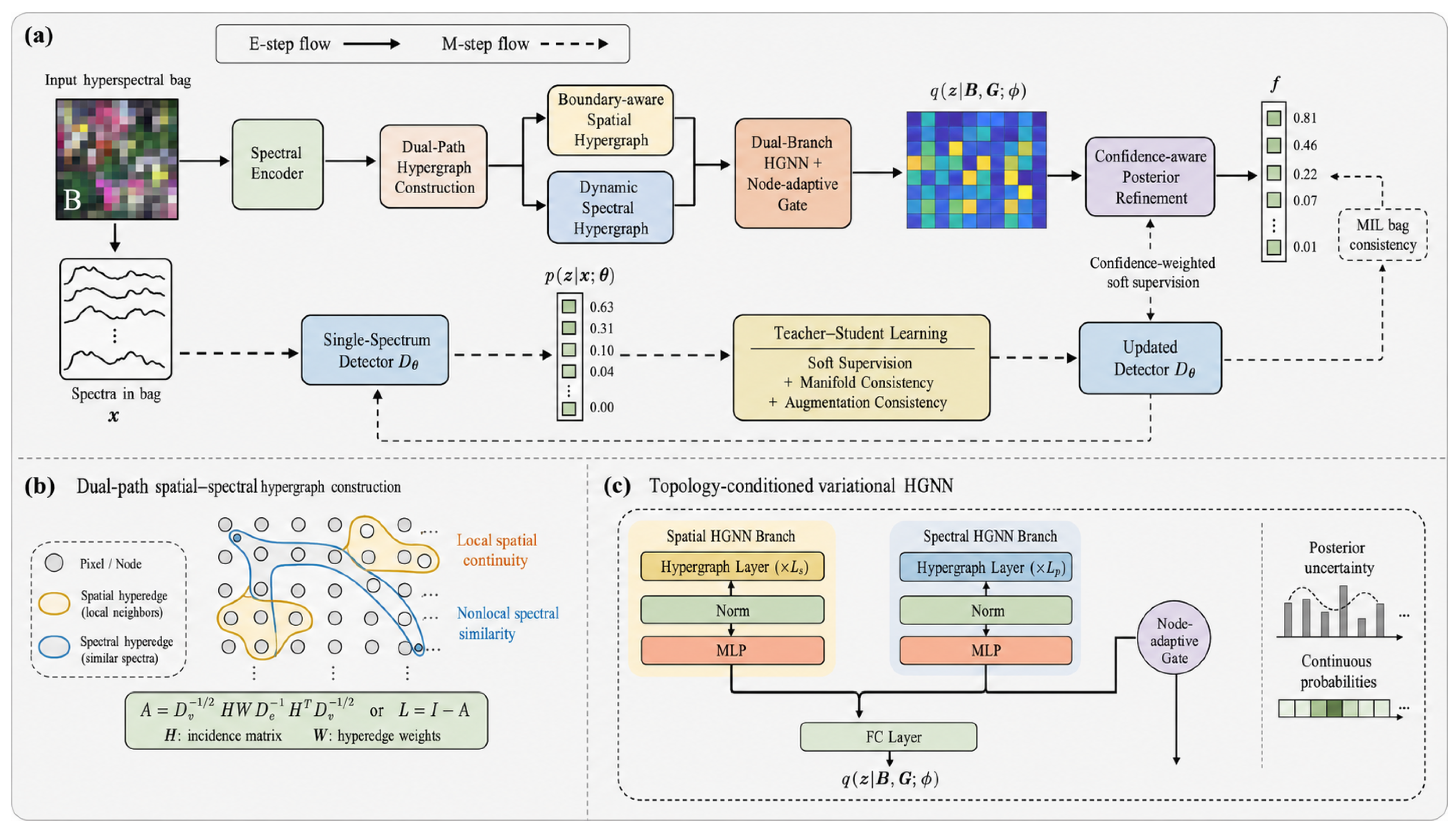
To address these challenges, we propose a Spatial–Spectral Topology-Regularized Variational Hypergraph Multiple-Instance Learning Network, termed Hyper-VMIL, for region-level weakly supervised HTD. Hyper-VMIL formulates latent target localization as a variational inference problem and represents each hyperspectral bag using two complementary hypergraphs. A boundary-aware spatial hypergraph organizes local neighborhoods according to two-dimensional coordinates and adjusts their propagation strengths using spectral differences. A dynamic spectral-manifold hypergraph connects spatially separated pixels with similar material characteristics in a learned embedding space. Unlike pairwise representations, each hyperedge can jointly associate an entire spatial patch or a group of spectrally similar instances, thereby capturing high-order spatial and spectral dependencies.

A dual-branch hypergraph neural network is used to parameterize the topology-conditioned mean-field posterior. The spatial and spectral branches propagate node information over their respective hypergraphs and are integrated through node-adaptive gates. The model can thus determine whether local spatial continuity or non-local spectral similarity provides more reliable evidence for each instance. Boundary-aware hyperedge weighting, residual propagation, and adaptive gating are introduced to prevent weak targets from being excessively smoothed into the background. The spatial–spectral hypergraph Laplacian is further incorporated into a regularized variational objective so that latent target posteriors remain consistent over reliable manifolds while preserving target boundaries and isolated target responses.

To mitigate the risk of information loss and error propagation (confirmation bias) often induced by premature hard pseudo-label binarization, we designed a confidence-aware topological posterior refinement mechanism as a principled motivation. Instead of enforcing rigid binary decisions at early optimization stages, the method preserves continuous target probabilities and estimates node-level confidence from posterior uncertainty. The latent target distribution is then refined under posterior-fidelity, spectral–spatial topology, and bag-label consistency constraints, which is intended to prevent ambiguous predictions from being prematurely reinforced as false positive supervision. High-confidence instances mainly retain their original predictions, whereas uncertain instances receive additional evidence from reliable topological neighbors, thereby theoretically limiting uncontrolled error accumulation.

Finally, a topology-teacher and pixel-student learning strategy was developed to bridge contextual inference and flexible deployment. The variational hypergraph network acts as a contextual teacher that estimates continuous instance posteriors from complete bags and their spectral–spatial structures. A pixel-level student detector takes only an individual spectrum as input and learns the teacher’s structured knowledge through confidence-weighted soft supervision, manifold consistency, and spectral perturbation consistency. The student does not directly perceive spatial topology at test time; instead, it learns a spectral decision function that approximates the topology-conditioned posterior. Consequently, Hyper-VMIL supports both a Context Mode, which explicitly constructs test hypergraphs for refined detection, and a Pixel Mode, which provides efficient and flexible single-spectrum inference. The main contributions of this work are summarized as follows:

• We propose a topology-regularized variational hypergraph multiple-instance framework that integrates region-level labels, high-order spectral–spatial structures, and instance-level target posteriors within a unified probabilistic learning formulation.
• We developed a boundary-aware dual-path hypergraph representation that characterizes local spatial continuity and non-local spectral manifolds. Node-adaptive gating, boundary-sensitive weights, and residual propagation jointly balance structural consistency and weak-target preservation.
• We developed confidence-aware continuous posterior refinement and topology-teacher–pixel-student collaborative learning. This strategy is specifically formulated to alleviate information loss and confirmation bias stemming from conventional hard pseudo-labeling, with its empirical effectiveness in stabilizing optimization and preventing error accumulation validated through ablation and dynamic trajectory experiments.

The remainder of this paper is organized as follows. Section 2 reviews recent studies on weakly supervised HTD, spectral–spatial representation, hypergraph learning, and knowledge distillation. Section 3 presents the proposed Hyper-VMIL framework and its optimization procedure. Section 4 reports comparative, ablation, and robustness experiments. Section 5 concludes the paper.

2. Related Work

2.1. Weakly Supervised Hyperspectral Target Detection

Recent HTD methods have employed spectral aggregation, Transformer-based dependency modeling, interpretable representation learning, variational background modeling, and self-supervised learning to improve target–background separation [2,3,4,5,6,7,8]. Graph-based fusion, spatial–spectral sparse encoding, and point-object detection architectures have further enhanced the representation of small targets and heterogeneous backgrounds [9,10,11]. However, many of these methods still rely on predefined target signatures, synthetic target samples, or accurate pixel-level annotations.

MIL provides a region-level weakly supervised alternative. With the MIL setting, a positive bag contains at least one target instance, whereas a negative bag contains only background instances. Recent weakly supervised HTD methods have explored metric learning, weak-label semantic modeling, spectral–spatial similarity-guided selection, latent target-location inference, and prototype memory [13,14,15,16,17]. These studies demonstrate that pixel detectors can be learned without precise instance annotations.

Nevertheless, correct bag prediction does not necessarily imply accurate instance localization, and instance-level learnability generally requires stronger conditions than bag-level classification [18,21]. Structure-aware MIL methods have shown that dependencies among instances can improve fine-grained prediction [22,23,24]. However, existing weakly supervised HTD methods mainly infer target locations from spectral embeddings, attention scores, or prototypes. The explicit two-dimensional organization of pixels is rarely incorporated into the latent posterior, while continuous instance scores are often converted into hard pseudo-labels. Hyper-VMIL instead introduces high-order spectral–spatial topology into variational instance inference and preserves continuous posterior information during optimization.

2.2. Spectral–Spatial Graph and Hypergraph Learning

Joint spectral–spatial modeling is important for detecting weak and subpixel targets. Transformer and self-supervised networks capture long-range spectral dependencies and neighborhood consistency [2,4,7,8]. Graph-based HTD methods further encode explicit relationships among pixels through graph convolution, feature fusion, sparse priors, or generative representation learning [9,10,25].

Specifically, hyperspectral spatial–spectral structures embody joint, multi-body (k-ary, $k\ge 3$) correlations that cannot be faithfully captured by conventional pairwise graphs or attention-based models. Standard graph neural networks model only dyadic (1-to-1) edges; decomposing an entire k-pixel spatial patch or a non-local spectral cluster into $\left({\displaystyle \genfrac{}{}{0pt}{}{k}{2}}\right)$ independent pairwise links introduces spurious intermediate interactions, distorts collective manifold geometry, and accelerates subpixel target over-smoothing across material boundaries. Meanwhile, Transformer-based self-attention computes dense, unconstrained pairwise token affinities without explicit geometric structure; under region-level weak supervision where subpixel targets are heavily diluted, all-to-all attention is readily swamped by redundant background tokens and cannot construct a closed-form graph Laplacian operator for topological posterior regularization. In contrast, hypergraphs uniquely represent non-decomposable group-level information: a single spatial hyperedge preserves the collective spatial co-occurrence of a patch, while a dynamic spectral hyperedge encapsulates non-local material manifold clusters simultaneously [19,26,27,28]. Furthermore, the resulting hypergraph Laplacian $L=I-D_v^{-1/2}HW{D}_e^{-1}{H}^{\top }{D}_v^{-1/2}$ provides a mathematically rigorous manifold regularizer ($z_i^{\top }{L}_i{z}_i$) to constrain uncertain instance posteriors during weakly supervised optimization.

Most existing hypergraph methods are designed for supervised classification and use hypergraphs as deterministic feature extractors. Their direct application to weakly supervised HTD is limited because instance labels in positive bags are unobserved. Moreover, uniform topology propagation may smooth isolated targets into the background or connect target-like background pixels incorrectly. Hyper-VMIL therefore incorporates boundary-aware spatial and spectral hypergraphs into latent posterior inference. The two topologies are modeled separately and fused through node-adaptive gates, while boundary-sensitive weights and residual connections alleviate unreliable propagation and over-smoothing.

2.3. Posterior Refinement and Knowledge Transfer

Weakly supervised HTD methods commonly generate instance supervision using attention responses, similarity measures, dynamic thresholds, or prototype assignments [14,15,16,17]. Although these strategies reduce label ambiguity, their performance depends strongly on early predictions. Incorrect high-confidence instances may be repeatedly used as supervision and reinforced during alternating optimization. In addition, binary pseudo-labels discard the distinction between confident targets, mixed pixels, and uncertain background responses.

Continuous posterior refinement provides a more informative alternative. Rather than immediately assigning hard labels, instance probabilities can be corrected according to their uncertainty and surrounding structure. Confident instances should largely preserve their original predictions, whereas ambiguous instances can receive additional evidence from reliable spectral and spatial neighbors. This selective refinement is particularly important for avoiding uncontrolled error propagation and excessive smoothing of weak targets.

Knowledge distillation has also been used to transfer spectral–spatial representations to lightweight HSI models [20,29,30]. However, most existing approaches address supervised classification, where teacher predictions are supported by reliable instance labels. In region-level weak supervision, the teacher itself estimates uncertain latent labels. Hyper-VMIL therefore refines the topology-conditioned teacher posterior using confidence, bag consistency, and boundary-aware topology before transferring it to a single-spectrum student. This design supports both topology-aware contextual detection and efficient pixel-level deployment.

3. Proposed Method

3.1. Overview and Problem Formulation

Given only region-level annotations, weakly supervised hyperspectral target detection aims to recover pixel-level target responses from bags containing both target and background instances. This problem is highly ambiguous because a positive bag only indicates the existence of at least one target, without revealing its location, number, or abundance. Moreover, weak and mixed targets may be difficult to distinguish from spectrally similar backgrounds when each pixel is considered independently.

To address this problem, as shown in Figure 1, Hyper-VMIL combines contextual instance inference and deployable pixel detection in a unified framework. It first constructs complementary spatial and spectral hypergraphs to describe high-order relations among pixels. A dual-branch hypergraph network then estimates a topology-conditioned variational posterior over the unknown instance labels. The posterior is further refined in a continuous form according to its confidence, bag-level consistency, and spectral–spatial topology. Finally, the refined contextual knowledge is transferred to a single-spectrum detector, enabling efficient pixel-level inference without requiring a hypergraph at deployment time.

Let the training set be

$$\mathcal{D}={\left\{({\mathcal{B}}_i,y_i)\right\}}_{i=1}^N,$$

(1)

where N is the number of bags and $y_i\in \{0,1\}$ is the region-level label of the ith bag. Each bag is represented as

$${\mathcal{B}}_i={\left\{(x_{ij},r_{ij})\right\}}_{j=1}^{n_i},$$

(2)

where $x_{ij}\in R^B$ denotes the spectrum of the jth pixel, $r_{ij}\in R^2$ is its spatial coordinate, B is the number of spectral bands, and $n_i$ is the number of instances in the bag.

Under the standard multiple-instance learning assumption,

$$y_i=\left\{\begin{array}{cc}1,\hfill & \exists j,z_{ij}=1,\hfill \\ 0,\hfill & z_{ij}=0,\forall j,\hfill \end{array}\right.$$

(3)

where $z_{ij}\in \{0,1\}$ is the unknown instance label. Thus, negative bags provide relatively reliable background information, whereas the target locations within positive bags must be inferred during training.

Hyper-VMIL models the latent instance distribution using a topology-conditioned mean-field posterior:

$$q_{\varphi }\left(z_i\mid {\mathcal{B}}_i,{\mathcal{G}}_i\right)={\displaystyle \prod _{j=1}^{n_i}}\mathrm{Bernoulli}(z_{ij};{\pi }_{ij}),$$

(4)

where $z_i={[z_{i1},\dots ,z_{i{n}_i}]}^{\top }$, ${\pi }_{ij}$ denotes the contextual target probability, and ${\mathcal{G}}_i$ represents the spectral–spatial topology of the bag.

In parallel, a single-spectrum detector produces

$$s_{ij}=p_{\theta }(z_{ij}=1\mid x_{ij})=D_{\theta }\left(x_{ij}\right).$$

(5)

In a probabilistic variational inference setting (Empirical Bayes framework), $s_{ij}$ serves as a parameterized empirical spectral prior (or context-free spectral prior). It represents the instance-level target probability conditioned strictly on the individual spectrum $x_{ij}$ prior to incorporating the high-order spatial–spectral hypergraph topology ${\mathcal{G}}_i$. During training, $s_{ij}$ provides an instance-level spectral prior for variational inference. During testing, $D_{\theta }$ can independently evaluate each spectrum without reconstructing the contextual topology. Therefore, ${\pi }_{ij}$ represents a context-aware estimate, whereas $s_{ij}$ represents a context-free spectral estimate.

To ground this probabilistic relationship within a rigorous variational inference framework, we formalize region-level weakly supervised HTD as a latent-variable generative model. For a bag ${\mathcal{B}}_i={\left\{(x_{ij},r_{ij})\right\}}_{j=1}^{n_i}$ with spatial–spectral hypergraph topology ${\mathcal{G}}_i=\{{\mathcal{G}}_i^{\mathrm{spa}},{\mathcal{G}}_i^{\mathrm{spe}}\}$, the joint generative distribution over the unobserved binary instance labels $z_i={[z_{i1},\dots ,z_{i{n}_i}]}^{\top }\in {\{0,1\}}^{n_i}$ and the observed bag label $y_i\in \{0,1\}$ is factorized as

$$p_{\theta }(y_i,z_i\mid X_i,{\mathcal{G}}_i)=p(y_i\mid z_i)p_{\theta }(z_i\mid X_i,{\mathcal{G}}_i).$$

(6)

Under the multiple-instance learning principle with label relaxation $ϵ\in (0,1)$, the bag-level likelihood $p(y_i\mid z_i)$ conditioned on latent instance labels $z_i$ is defined by a Bernoulli distribution:

$$p(y_i\mid z_i)={\left[1-(1-ϵ){\displaystyle \prod _{j=1}^{n_i}}(1-z_{ij})\right]}^{y_i}{\left[(1-ϵ){\displaystyle \prod _{j=1}^{n_i}}(1-z_{ij})\right]}^{1-y_i}.$$

(7)

Rather than assuming independent and identically distributed instances, the prior distribution $p_{\theta }(z_i\mid X_i,{\mathcal{G}}_i)$ over latent variables $z_i$ is formulated as a Hypergraph Markov Random Field (Hypergraph MRF) Gibbs distribution conditioned on the single-spectrum detector $D_{\theta }$ and the dual hypergraph Laplacians $L_i^{\mathrm{spa}},L_i^{\mathrm{spe}}$:

$$\begin{array}{cc}\hfill \begin{array}{c}\hfill p_{\theta }(z_i\mid X_i,{\mathcal{G}}_i)\end{array}& \begin{array}{c}\hfill =\end{array}\begin{array}{c}\hfill {\displaystyle \frac{1}{Z(\theta ,{\mathcal{G}}_i)}}\exp ({\displaystyle \sum _{j=1}^{n_i}}\left[z_{ij}\log {\displaystyle \frac{s_{ij}}{1-s_{ij}}}+\log (1-s_{ij})\right]\end{array}\hfill \\ \hfill & \begin{array}{c}\hfill -{\displaystyle \frac{{\lambda }_{\mathrm{spa}}}{2}}{z}_i^{\top }{L}_i^{\mathrm{spa}}{z}_i-{\displaystyle \frac{{\lambda }_{\mathrm{spe}}}{2}}{z}_i^{\top }{L}_i^{\mathrm{spe}}{z}_i),\end{array}\hfill \end{array}$$

(8)

where $Z(\theta ,{\mathcal{G}}_i)$ is the partition function. This Hypergraph MRF prior explicitly anchors the context-free spectral detector $s_{ij}=D_{\theta }\left(x_{ij}\right)$ alongside spatial–spectral hypergraph Laplacians $L_i^{\mathrm{spa}}$ and $L_i^{\mathrm{spe}}$, ensuring that spectrally similar and spatially adjacent instances are encouraged to maintain consistent target states prior to contextual variational inference.

3.2. Dual-Path Spatial–Spectral Hypergraph

A target pixel may receive useful evidence from both its local spatial neighborhood and spectrally similar pixels at distant locations. However, these two relations have different meanings and may not always be equally reliable. Hyper-VMIL therefore represents each bag using two complementary hypergraphs:

$${\mathcal{G}}_i=\left\{{\mathcal{G}}_i^{\mathrm{spa}},{\mathcal{G}}_i^{\mathrm{spe}}\right\}.$$

(9)

The spatial hypergraph models local geometric continuity, whereas the spectral hypergraph describes non-local material similarity. Unlike ordinary graphs that connect pairs of nodes, a hyperedge can jointly associate a group of pixels and is therefore suitable for representing spatial patches and spectral-neighbor groups.

3.2.1. Boundary-Aware Spatial Hypergraph

For each center node c, its $k_{\mathrm{spa}}$ spatially nearest pixels form a hyperedge $e_c^{\mathrm{spa}}$. A topology constructed only from coordinates may connect a weak target with many surrounding background pixels. To suppress unreliable cross-boundary propagation, the soft incidence value is defined jointly by spatial distance and spectral difference:

$$\begin{array}{cc}\hfill H_{j,e_c}^{\mathrm{spa}}=& \mathbb{I}\left[j\in {\mathcal{N}}^{\mathrm{spa}}\left(c\right)\right]\exp \left(-{\displaystyle \frac{\parallel r_{ij}-r_{ic}{\parallel }_2^2}{2{\sigma }_r^2}}\right)\hfill \\ \hfill & \times \exp \left(-{\displaystyle \frac{\parallel x_{ij}-x_{ic}{\parallel }_2^2}{2{\sigma }_x^2}}\right),\hfill \end{array}$$

(10)

where ${\mathcal{N}}^{\mathrm{spa}}\left(c\right)$ denotes the spatial neighborhood of node c. The coordinate kernel favors local interactions, while the spectral kernel reduces the membership of pixels with strong spectral discontinuities.

It is worth clarifying the fundamental distinction between this formulation and conventional boundary-aware pairwise graph weighting methods. Traditional boundary-aware graphs define scalar affinities over independent dyadic edges ($W_{jk}$), which decomposes a local spatial patch into pairwise interactions and discards collective multi-pixel geometry. In contrast, Equation (10) defines a continuous hyperedge incidence entry $H_{j,e_c}^{\mathrm{spa}}\in [0,1]$ that characterizes the continuous membership degree of node j within the collective, non-dyadic hyperedge $e_c$. With the normalized hypergraph operator $A^{\mathrm{spa}}=D_v^{-1/2}HW{D}_e^{-1}{H}^{\top }{D}_v^{-1/2}$, this formulation enforces a two-stage message-passing mechanism (node-to-hyperedge aggregation followed by hyperedge-to-node broadcast). Consequently, spectrally inconsistent boundary pixels are quadratically attenuated in both aggregation and broadcasting phases, effectively preventing cross-boundary noise leakage while preserving the holistic spatial support of homogeneous interior patches. Furthermore, the resulting hypergraph Laplacian $L^{\mathrm{spa}}=I-A^{\mathrm{spa}}$ is directly integrated into the variational objective to penalize topological inconsistency under Bernoulli posterior uncertainty conditions.

3.2.2. Dynamic Spectral-Manifold Hypergraph

The spatial hypergraph cannot directly associate pixels belonging to the same material when they are spatially separated. A spectral hypergraph is therefore constructed in a learned embedding space:

$$h_{ij}=E_{\overline{\psi }}\left(x_{ij}\right),$$

(11)

where $E_{\overline{\psi }}$ is an exponential-moving-average encoder. Its parameters are updated as

$$\overline{\psi }\leftarrow m\overline{\psi }+(1-m)\psi ,$$

(12)

where $\psi$ denotes the online encoder parameters and m is the momentum coefficient. The slowly varying encoder produces more stable feature neighborhoods than directly using rapidly updated online embeddings.

For each center node, its $k_{\mathrm{spe}}$ nearest neighbors in the embedding space form a spectral hyperedge. The corresponding incidence value is

$$H_{j,e_c}^{\mathrm{spe}}=\mathbb{I}\left[j\in {\mathcal{N}}^{\mathrm{spe}}\left(c\right)\right]\exp \left(-{\displaystyle \frac{\parallel h_{ij}-h_{ic}{\parallel }_2^2}{2{\sigma }_h^2}}\right).$$

(13)

This topology connects spatially distant pixels with similar material characteristics and complements the local spatial structure. Since the embedding space gradually evolves during training, the spectral hypergraph is reconstructed every R iterations rather than after every gradient update, thereby reducing oscillations in neighborhood assignments.

For either hypergraph, the normalized propagation operator is

$$A=D_v^{-{\displaystyle \frac{1}{2}}}HW{D}_e^{-1}{H}^{\top }{D}_v^{-{\displaystyle \frac{1}{2}}},$$

(14)

where $H\in {\mathbb{R}}^{n_i\times n_i}$ denotes the soft incidence matrix. The diagonal node-degree matrix $D_v\in {\mathbb{R}}^{n_i\times n_i}$ and hyperedge-degree matrix $D_e\in {\mathbb{R}}^{n_i\times n_i}$ are explicitly defined by $D_v(j,j)={\sum }_{e=1}^{n_i}{H}_{j,e}$ and $D_e(e,e)={\sum }_{j=1}^{n_i}{H}_{j,e}$, respectively. Following the standard hypergraph spectral formulation, the hyperedge weight matrix is set to the identity matrix $W=I_{n_i}$. The corresponding normalized Laplacian is

$$L=I-A.$$

(15)

3.3. Topology-Conditioned Variational Inference

The spatial and spectral hypergraphs are processed by two independent branches so that their distinct relational properties can be retained. For a hyperspectral bag ${\mathcal{B}}_i$ with spectral matrix $X_i={[x_{i1},\dots ,x_{i{n}_i}]}^{\top }\in {\mathbb{R}}^{n_i\times B}$, the initial node representations are initialized via the online spectral encoder: $U_{\mathrm{spa}}^{\left(0\right)}=U_{\mathrm{spe}}^{\left(0\right)}=E_{\psi }\left(X_i\right)\in {\mathbb{R}}^{n_i\times d_0}$. For $t\in \{\mathrm{spa},\mathrm{spe}\}$, the lth hypergraph layer is defined as

$$U_t^{(l+1)}=\sigma \left(A_t{U}_t^{\left(l\right)}{W}_t^{\left(l\right)}+U_t^{\left(l\right)}{R}_t^{\left(l\right)}\right),$$

(16)

where $W_t^{\left(l\right)}$ is the contextual transformation matrix and $R_t^{\left(l\right)}$ is a residual projection. The first term aggregates features through hypergraph connectivity, while the residual term retains instance-specific spectral information and reduces over-smoothing. Let $u_{ij}^{\mathrm{spa}}$ and $u_{ij}^{\mathrm{spe}}$ denote the final representations of the two branches. Because spatial continuity and spectral similarity may have different reliability for different pixels, they are fused through a node-adaptive gate:

$$\begin{array}{cc}\hfill g_{ij}& =\sigma \left({\mathrm{MLP}}_g\left[u_{ij}^{\mathrm{spa}};u_{ij}^{\mathrm{spe}}\right]\right),\hfill \end{array}$$

(17)

$$\begin{array}{cc}\hfill u_{ij}& =g_{ij}{u}_{ij}^{\mathrm{spa}}+(1-g_{ij})u_{ij}^{\mathrm{spe}},\hfill \end{array}$$

(18)

$$\begin{array}{cc}\hfill {\pi }_{ij}\left(\varphi \right)& =\sigma \left(w_q^{\top }{u}_{ij}+b_q\right).\hfill \end{array}$$

(19)

The gate allows the model to emphasize spatial evidence in homogeneous regions and spectral evidence near boundaries or within spatially discontinuous target regions. Here, we collect all learnable parameters of the contextual posterior branch into $\varphi =\{\psi ,{\{W_t^{\left(l\right)},R_t^{\left(l\right)}\}}_{l,t},{\mathsf{\Theta }}_g,w_q,b_q\}$, where ${\mathsf{\Theta }}_g$ denotes the weights of ${\mathrm{MLP}}_g$.

To optimize the parameters $\varphi$ of the topology-conditioned posterior $q_{\varphi }(z_i\mid X_i,{\mathcal{G}}_i)={\prod }_{j=1}^{n_i}\mathrm{Bernoulli}(z_{ij};{\pi }_{ij}\left(\varphi \right))$, evaluating the exact log marginal likelihood $\log p_{\theta }(y_i\mid X_i,{\mathcal{G}}_i)=\log {\sum }_{z_i}{p}_{\theta }(y_i,z_i\mid X_i,{\mathcal{G}}_i)$ directly is computationally intractable due to the combinatorial summation over $2^{n_i}$ latent states. We therefore construct the Evidence Lower Bound (ELBO) on the marginal log-likelihood as follows:

$$\begin{array}{cc}\hfill \log p_{\theta }(y_i\mid X_i,{\mathcal{G}}_i)& \ge {\mathbb{E}}_{q_{\varphi }\left(z_i\right)}\left[\log {\displaystyle \frac{p_{\theta }(y_i,z_i\mid X_i,{\mathcal{G}}_i)}{q_{\varphi }(z_i\mid X_i,{\mathcal{G}}_i)}}\right]\hfill \\ \hfill & =\underset{\mathrm{Term}\mathrm{I}:\mathrm{Expected}\text{Log-Likelihood}}{\underbrace{{\mathbb{E}}_{q_{\varphi }\left(z_i\right)}\left[\log p(y_i\mid z_i)\right]}}-\underset{\mathrm{Term}\mathrm{II}:\mathrm{Prior}\mathrm{KL}\mathrm{Divergence}}{\underbrace{D_{\mathrm{KL}}\left(q_{\varphi }(z_i\mid X_i,{\mathcal{G}}_i)\parallel p_{\theta }(z_i\mid X_i,{\mathcal{G}}_i)\right)}}.\hfill \end{array}$$

(20)

Equivalence of Term I to ${\mathcal{L}}_{\mathrm{bag}}^q$: With the mean-field Bernoulli posterior $q_{\varphi }$, the expectation of the product term in Equation (7) is evaluated analytically:

$${\mathbb{E}}_{q_{\varphi }}\left[{\displaystyle \prod _{j=1}^{n_i}}(1-z_{ij})\right]={\displaystyle \prod _{j=1}^{n_i}}{\mathbb{E}}_{q_{\varphi }}[1-z_{ij}]={\displaystyle \prod _{j=1}^{n_i}}(1-{\pi }_{ij}\left(\varphi \right)).$$

(21)

Defining the variational bag target prediction as ${\widehat{y}}_i^q=1-(1-ϵ){\prod }_{j=1}^{n_i}(1-{\pi }_{ij}\left(\varphi \right))$, the expected log-likelihood expands strictly to

$$\begin{array}{cc}\hfill {\mathbb{E}}_{q_{\varphi }\left(z_i\right)}\left[\log p(y_i\mid z_i)\right]& =y_i\log {\widehat{y}}_i^q+(1-y_i)\log (1-{\widehat{y}}_i^q)=-{\mathcal{L}}_{\mathrm{bag}}^q.\hfill \end{array}$$

(22)

This proves that the bag-level loss ${\mathcal{L}}_{\mathrm{bag}}^q$ is strictly derived from the expected log-likelihood of the variational ELBO.

Equivalence of Term II to Topology Regularization and ${\mathcal{L}}_{\mathrm{KL}}$: Substituting the Hypergraph MRF prior (Equation (8)) and the mean-field posterior into the KL divergence term yields

$$\begin{array}{cc}\hfill D_{\mathrm{KL}}\left(q_{\varphi }\parallel p_{\theta }\right)& ={\mathbb{E}}_{q_{\varphi }}\left[\log q_{\varphi }\left(z_i\right)-\log p_{\theta }(z_i\mid X_i,{\mathcal{G}}_i)\right]\hfill \\ \hfill & ={\displaystyle \sum _{j=1}^{n_i}}{D}_{\mathrm{KL}}\left(\mathrm{Bern}\left({\pi }_{ij}\left(\varphi \right)\right)\parallel \mathrm{Bern}\left(s_{ij}\right)\right)\hfill \\ \hfill & +{\displaystyle \frac{{\lambda }_{\mathrm{spa}}}{2}}{\mathbb{E}}_{q_{\varphi }}\left[z_i^{\top }{L}_i^{\mathrm{spa}}{z}_i\right]+{\displaystyle \frac{{\lambda }_{\mathrm{spe}}}{2}}{\mathbb{E}}_{q_{\varphi }}\left[z_i^{\top }{L}_i^{\mathrm{spe}}{z}_i\right]\hfill \\ \hfill & +\log Z(\theta ,{\mathcal{G}}_i).\hfill \end{array}$$

(23)

Under the Bernoulli posterior variance expansion with diagonal covariance matrix ${\mathrm{Cov}}_{q_{\varphi }}\left(z_i\right)=\mathrm{Diag}({\pi }_i\left(\varphi \right)\odot (1-{\pi }_i\left(\varphi \right)))$, the expected topology terms expand analytically as

$${\mathbb{E}}_{q_{\varphi }}\left[z_i^{\top }{L}_i^t{z}_i\right]={\pi }_i{\left(\varphi \right)}^{\top }{L}_i^t{\pi }_i\left(\varphi \right)+\mathrm{tr}\left[L_i^t\mathrm{Diag}({\pi }_i\left(\varphi \right)\odot (1-{\pi }_i\left(\varphi \right)))\right]\triangleq {\mathcal{R}}_t,t\in \{\mathrm{spa},\mathrm{spe}\}.$$

(24)

Here, the expansion reveals two distinct physical mechanisms: the quadratic term ${\pi }_i{\left(\varphi \right)}^{\top }{L}_i^t{\pi }_i\left(\varphi \right)$ enforces topological smoothness across hypergraph hyperedges by penalizing differences between connected posterior means, whereas the trace term $\mathrm{tr}\left[L_i^t\mathrm{Diag}({\pi }_i\left(\varphi \right)\odot (1-{\pi }_i\left(\varphi \right)))\right]={\sum }_{j=1}^{n_i}{\left(L_i^t\right)}_{jj}{\pi }_{ij}\left(\varphi \right)(1-{\pi }_{ij}\left(\varphi \right))$ acts as an instance-level variance penalty. Because the diagonal elements of the normalized hypergraph Laplacian are positive (${\left(L_i^t\right)}_{jj}>0$), minimizing this trace term explicitly penalizes instance-level Bernoulli uncertainty, thereby driving the posterior predictions ${\pi }_{ij}\left(\varphi \right)$ toward confident binary decisions (0 or 1).

3.4. Confidence-Aware Posterior Refinement

Although the variational posterior integrates multiple sources of evidence, some predictions may remain ambiguous because of mixed spectra, noisy embeddings, or imperfect hyperedges. Directly converting ${\pi }_{ij}$ into a hard pseudo-label would discard uncertainty and may reinforce early errors. Hyper-VMIL therefore refines the posterior while retaining its continuous probability form.

The confidence of an instance is estimated from normalized Bernoulli entropy:

$$\begin{array}{cc}\hfill \mathcal{H}\left({\pi }_{ij}\right)& =-{\pi }_{ij}\log {\pi }_{ij}-(1-{\pi }_{ij})\log (1-{\pi }_{ij}),\hfill \end{array}$$

(25)

$$\begin{array}{cc}\hfill c_{ij}& =1-{\displaystyle \frac{\mathcal{H}\left({\pi }_{ij}\right)}{\log 2}}.\hfill \end{array}$$

(26)

Predictions near zero or one receive high confidence, whereas predictions near $0.5$ are considered uncertain and can be corrected more strongly.

For each bag, the refined posterior $f_i\in {[0,1]}^{n_i}$ is obtained by

$$\begin{array}{cc}\hfill f_i^{*}=\arg \underset{f_i}{\min }& {(f_i-{\pi }_i)}^{\top }{C}_i(f_i-{\pi }_i)\hfill \\ \hfill & +{\mu }_{\mathrm{spa}}{f}_i^{\top }{L}_i^{\mathrm{spa}}{f}_i+{\mu }_{\mathrm{spe}}{f}_i^{\top }{L}_i^{\mathrm{spe}}{f}_i\hfill \\ \hfill & +\xi {\mathcal{L}}_{\mathrm{bag}}(f_i,y_i),f_i\in {[0,1]}^{n_i},\hfill \end{array}$$

(27)

where

$$C_i=\mathrm{Diag}(c_{i1}+\delta ,\dots ,c_{i{n}_i}+\delta )$$

(28)

and $\delta$ is a small positive constant.

It is important to emphasize the functional distinction of Equation (27) between the training and testing phases. During model training, weak bag labels $y_i$ are available, and setting $\xi >0$ provides a weak bag-level consistency constraint to prevent refined posteriors from drifting away from observed annotations. Conversely, during test-time inference on unseen scenes, ground-truth bag labels $y_i$ are strictly unavailable. Therefore, for all test evaluations, we strictly set $\xi =0$, removing the term $\xi {\mathcal{L}}_{\mathrm{bag}}(f_i,y_i)$ completely. In this label-free test mode, Equation (27) functions purely as an unsupervised manifold-regularized probability refinement process.

The first term preserves reliable posterior predictions. The spatial and spectral Laplacian terms provide complementary corrections to uncertain instances, while the final term maintains consistency with the observed bag label. The bag probability associated with the refined posterior is

$${\widehat{y}}_i^f=1-(1-ϵ){\displaystyle \prod _{j=1}^{n_i}}(1-f_{ij}).$$

(29)

To solve the constrained convex optimization problem in Equation (27) efficiently, we employ Projected Gradient Descent (PGD) with analytical gradient evaluation. Denoting the objective in Equation (27) by $\mathcal{J}\left(f_i\right)$, its exact gradient with respect to $f_i$ is derived as

$${\nabla }_{f_i}\mathcal{J}\left(f_i\right)=2C_i(f_i-{\pi }_i)+2\left({\mu }_{\mathrm{spa}}{L}_i^{\mathrm{spa}}+{\mu }_{\mathrm{spe}}{L}_i^{\mathrm{spe}}\right)f_i+\xi g_{\mathrm{bag}}\left(f_i\right),$$

(30)

where the j-th entry of the bag loss gradient vector $g_{\mathrm{bag}}\left(f_i\right)\in {\mathbb{R}}^{n_i}$ evaluates analytically to

$${\left[g_{\mathrm{bag}}\left(f_i\right)\right]}_j={\displaystyle \frac{\partial {\mathcal{L}}_{\mathrm{bag}}(f_i,y_i)}{\partial f_{ij}}}={\displaystyle \frac{{\widehat{y}}_i^f-y_i}{{\widehat{y}}_i^f(1-{\widehat{y}}_i^f)}}·(1-ϵ){\displaystyle \prod _{k\ne j}^{n_i}}(1-f_{ik}).$$

(31)

Starting from the initial contextual posterior $f_i^{\left(0\right)}={\pi }_i$, the refined posterior is updated iteratively over $T_{\mathrm{refine}}=10$ steps with a fixed step size $\eta =0.05$ using Euclidean projection onto the probability simplex ${[0,1]}^{n_i}$:

$$f_i^{(t+1)}=\mathrm{clip}\left(f_i^{\left(t\right)}-\eta {\nabla }_{f_i}\mathcal{J}\left(f_i^{\left(t\right)}\right),0,1\right),t=0,\dots ,T_{\mathrm{refine}}-1.$$

(32)

Equation (27) can be solved using a small number of projected-gradient iterations. Unlike conventional hard pseudo-labeling, the result retains both target probability and uncertainty information. Moreover, the confidence-weighted fidelity term prevents topology regularization from uniformly smoothing all nodes.

While the confidence-weighted fidelity term ${(f_i-{\pi }_i)}^{\top }{C}_i(f_i-{\pi }_i)$ prevents uniform over-smoothing, entropy-based confidence measures predictive certainty rather than ground-truth correctness. If left unconstrained, an isolated false-positive prediction with high certainty (${\pi }_{ij}\approx 1$, $c_{ij}\to 1$) could receive a large fidelity weight and risk entrenching confirmation bias. In Hyper-VMIL, such confidently incorrect predictions are systematically rectified through two mathematically coupled mechanisms: collective topological overruling and orthogonal spectral prior anchoring.

First, CTPR performs a globally coupled optimization over the entire bag manifold in Equation (27). When an isolated background pixel j yields an erroneous high-confidence posterior ${\pi }_{ij}\approx 0.95$, its surrounding spatial neighbors and spectral k-NN peers within the incident hyperedges remain predominantly background (${\pi }_{ik}\approx 0$). In this setting, maintaining a large refined value $f_{ij}^{*}\approx 0.95$ creates steep gradients across incident hyperedges, incurring an extreme quadratic energy penalty $f_i^{\top }({\mu }_{\mathrm{spa}}{L}_i^{\mathrm{spa}}+{\mu }_{\mathrm{spe}}{L}_i^{\mathrm{spe}})f_i={\sum }_{e}w\left(e\right){\sum }_{u,v\in e}{\displaystyle \frac{{(f_{iu}-f_{iv})}^2}{\delta \left(e\right)}}$. Because the topological penalty scales quadratically with the discrepancy across all hyperedge members, the collective consensus of the entire hyperedge neighborhood mathematically overrules the single-node fidelity weight $c_{ij}$, pulling $f_{ij}^{*}$ back down toward the true background manifold.

Second, the contextual posterior ${\pi }_i\left(\varphi \right)$ is strictly anchored to the single-spectrum detector prior $s_{ij}=D_{\theta }\left(x_{ij}\right)$ via mode-seeking forward KL divergence in Equation (23). The detector $D_{\theta }$ evaluates the physical spectrum $x_{ij}$ on a single-pixel basis, free from spatial neighborhood context. With the zero-forcing property of forward KL divergence (${\lim }_{s_{ij}\to 0}{D}_{\mathrm{KL}}(\mathrm{Bern}\left({\pi }_{ij}\right)\parallel \mathrm{Bern}\left(s_{ij}\right))=+\infty$ if ${\pi }_{ij}>0$), any spurious contextual activation on a background pixel ($s_{ij}\to 0$) is heavily penalized during the alternating E-step, forcing ${\pi }_{ij}\to 0$ in subsequent GEM iterations and breaking the confirmation bias feedback loop.

3.5. Topology-Teacher and Pixel-Student Learning

The hypergraph posterior uses the complete bag and its spatial–spectral relations and is therefore regarded as a contextual teacher. The single-spectrum detector acts as a pixel student. Since the teacher itself is learned from weak labels, its predictions are not treated as equally reliable ground truth. Instead, the refined posterior is transferred according to its confidence.

The confidence of the refined posterior is

$${\tilde{c}}_{ij}=1-{\displaystyle \frac{\mathcal{H}\left(f_{ij}\right)}{\log 2}},$$

(33)

and the confidence-weighted soft supervision is

$${\mathcal{L}}_{\mathrm{soft}}=-\sum _{i,j}{w}_{ij}\left[f_{ij}\log s_{ij}+(1-f_{ij})\log (1-s_{ij})\right],$$

(34)

where

$$w_{ij}=\tau +(1-\tau ){\tilde{c}}_{ij},0<\tau <1.$$

(35)

The lower bound $\tau >0$ plays a vital role in preventing confirmation bias against weakly expressed targets. For heavily mixed or subpixel targets where spectral overlap induces moderate posterior uncertainty ($f_{ij}\approx 0.5,{\tilde{c}}_{ij}\approx 0$), setting $\tau >0$ guarantees that genuine target responses retain a non-zero distillation gradient ($w_{ij}\ge \tau$), preventing faint target features from being completely discarded during student training.

The student is additionally constrained by the original bag labels:

$$\begin{array}{cc}\hfill {\widehat{y}}_i^s& =1-(1-ϵ){\displaystyle \prod _{j=1}^{n_i}}(1-s_{ij}),\hfill \end{array}$$

(36)

$$\begin{array}{cc}\hfill {\mathcal{L}}_{\mathrm{bag}}^s& =-\sum _i\left[y_i\log {\widehat{y}}_i^s+(1-y_i)\log (1-{\widehat{y}}_i^s)\right].\hfill \end{array}$$

(37)

Crucially, the direct bag-level supervision ${\mathcal{L}}_{\mathrm{bag}}^s$ provides an indispensable safety net that prevents the student from unconditionally memorizing incorrect teacher predictions. For negative bags ($y_i=0$), ${\mathcal{L}}_{\mathrm{bag}}^s$ enforces ${\prod }_{j=1}^{n_i}(1-s_{ij})\to 1$, which strictly penalizes all instance responses $s_{ij}\to 0$. Even if the contextual teacher momentarily transfers a false-positive pseudo-label on a negative bag, the loss ${\mathcal{L}}_{\mathrm{bag}}^s$ acts as a hard constraint anchored to the ground-truth weak supervision, directly suppressing student false alarms and preventing error accumulation across M-step optimization.

To transfer structural information during training, the student predictions are regularized over the two hypergraphs:

$${\mathcal{L}}_{\mathrm{man}}=\sum _i{s}_i^{\top }\left(L_i^{\mathrm{spa}}+L_i^{\mathrm{spe}}\right)s_i.$$

(38)

This regularizer encourages the student decision function to approximate the topology-conditioned teacher along reliable training manifolds. It is used only during training and does not imply that the student directly observes test-scene topology.

We further impose prediction consistency under weak spectral perturbation conditions:

$${\mathcal{L}}_{\mathrm{aug}}=\sum _{i,j}{D}_{\mathrm{SKL}}\left[D_{\theta }\left(x_{ij}\right),D_{\theta }\left({\tilde{x}}_{ij}\right)\right],$$

(39)

where $D_{\mathrm{SKL}}(u,v)=D_{\mathrm{KL}}(\mathrm{Bern}\left(u\right)\parallel \mathrm{Bern}\left(v\right))+D_{\mathrm{KL}}(\mathrm{Bern}\left(v\right)\parallel \mathrm{Bern}\left(u\right))$ is the symmetric Kullback–Leibler divergence between two scalar Bernoulli probabilities $u=D_{\theta }\left(x_{ij}\right)$ and $v=D_{\theta }\left({\tilde{x}}_{ij}\right)$, expanding analytically to

$$D_{\mathrm{SKL}}(u,v)=(u-v)\log \left({\displaystyle \frac{u(1-v)}{v(1-u)}}\right).$$

(40)

The perturbed spectrum ${\tilde{x}}_{ij}$ is generated via stochastic spectral transformations: zero-mean Gaussian noise injection $ϵ$∼$\mathcal{N}(0,{\sigma }_{\mathrm{noise}}^{2}I)$ with ${\sigma }_{\mathrm{noise}}=0.02$, random band erasure with masking probability $p_{\mathrm{mask}}=0.15$, and random global intensity scaling with multiplicative factor ${\rho }_{\mathrm{scale}}$∼$\mathcal{U}(0.9,1.1)$.

The complete student objective is

$${\mathcal{L}}_M={\mathcal{L}}_{\mathrm{soft}}+\alpha {\mathcal{L}}_{\mathrm{bag}}^s+\rho {\mathcal{L}}_{\mathrm{man}}+\kappa {\mathcal{L}}_{\mathrm{aug}}.$$

(41)

3.6. Optimization and Inference

The overall optimization is formulated as a Generalized Variational Expectation-Maximization (GEM) framework [31]. Rather than alternating between heuristic discriminative networks, the algorithm alternately optimizes the variational posterior parameters $\varphi$ and the generative student detector parameters $\theta$ to optimize the regularized ELBO bound. The exact parameter partitioning and gradient update schedule per mini-batch are detailed below:

• Variational E-Step (Updating Contextual Posterior $\varphi$): With the student detector parameters $\theta$ held fixed, the empirical spectral prior $s_{ij}=D_{\theta }\left(x_{ij}\right)$ is evaluated as a detached constant tensor ($\mathrm{detach}\left(s_{ij}\right)$). We perform $K_E=1$ mini-batch gradient step on teacher parameters $\varphi =\{\psi ,{\{W_t^{\left(l\right)},R_t^{\left(l\right)}\}}_{l,t},{\mathsf{\Theta }}_g,w_q,b_q\}$ to minimize the negative Evidence Lower Bound ($-\mathrm{ELBO}\left(\varphi \right)$, derived in Equations (20)–(24)) using Adam.
• Continuous Posterior Refinement (Solving $f_i^{*}$): Given the inferred posterior probabilities ${\pi }_i\left(\varphi \right)$ as detached inputs, the continuous refined posterior $f_i^{*}$ is solved via $T_{\mathrm{refine}}=10$ iterations of Projected Gradient Descent (PGD) according to Equation (32). This step executes non-parametric manifold smoothing on the simplex ${[0,1]}^{n_i}$ without updating any neural network weights.
• Generalized M-Step (Updating Single-Spectrum Student $\theta$): With teacher parameters $\varphi$ held fixed, the refined posterior targets $f_i^{*}$ and confidence weights ${\tilde{c}}_{ij}$ are treated as detached supervision constants ($\mathrm{detach}\left(f_i^{*}\right),\mathrm{detach}\left({\tilde{c}}_{ij}\right)$). We execute $K_M=1$ mini-batch gradient step on student detector parameters $\theta$ to minimize ${\mathcal{L}}_M$ (Equation (41)).
• EMA Encoder and Hypergraph Updates: Following each mini-batch, the momentum encoder parameters are updated via $\overline{\psi }\leftarrow m\overline{\psi }+(1-m)\psi$ ($m=0.99$). The dynamic spectral-manifold hypergraph ${\mathcal{G}}_i^{\mathrm{spe}}$ is reconstructed every $R=5$ epochs in the 64-D embedding space, ensuring topological stability.

Hyper-VMIL supports two complementary inference modes. In Pixel Mode, only the student detector is used:

$$d_j^{\mathrm{pix}}=D_{\theta }\left(x_j\right).$$

(42)

This mode requires neither spatial coordinates nor test-scene hypergraph construction and is suitable for fast or resource-constrained deployment.

In Context Mode, spatial and spectral hypergraphs are constructed for the test region, and the refined teacher posterior $f_j$ is combined with the student prediction $s_j$:

$$d_j^{\mathrm{ctx}}=\gamma f_j+(1-\gamma )s_j,$$

(43)

where $\gamma \in [0,1]$ balances contextual and single-spectrum evidence.

Crucially, to enforce a strictly label-free testing protocol and eliminate any possibility of test-label leakage, posterior refinement during context-mode inference is performed by setting $\xi =0$ in Equation (27). With this setting, the test-time continuous posterior refinement reduces to solving the following unsupervised optimization problem without relying on any test bag annotations:

$$\begin{array}{cc}\hfill \begin{array}{c}\hfill f_i^{*}\end{array}& \begin{array}{c}\hfill =\end{array}\begin{array}{c}\hfill \arg \underset{f_i\in {[0,1]}^{n_i}}{\min }{(f_i-{\pi }_i)}^{\top }{C}_i(f_i-{\pi }_i)\end{array}\hfill \\ \hfill & \begin{array}{c}\hfill +{\mu }_{\mathrm{spa}}{f}_i^{\top }{L}_i^{\mathrm{spa}}{f}_i+{\mu }_{\mathrm{spe}}{f}_i^{\top }{L}_i^{\mathrm{spe}}{f}_i.\end{array}\hfill \end{array}$$

(44)

This optimization relies exclusively on the model’s predicted posterior fidelity, posterior confidence $C_i$, and the unsupervised spatial–spectral hypergraph Laplacians ($L_i^{\mathrm{spa}}$ and $L_i^{\mathrm{spe}}$) constructed from the test scene.

4. Experiments

To comprehensively evaluate the performance, robustness, and computational efficiency of the proposed Hyper-VMIL framework, extensive experiments were conducted on three benchmark hyperspectral detection datasets, including one simulated dataset and two complex real-world airborne datasets.

4.1. Datasets and Bag Construction

• Simulated ASTER Dataset: Following the standard simulation protocol in weakly supervised hyperspectral target detection (HTD), six endmembers were selected from the USGS/ASTER spectral library [32]. Red Slate was designated as the target material, while the remaining five were used as backgrounds. Hyperspectral mixtures were synthesized using the Linear Mixing Model (LMM) [33] with Dirichlet-distributed abundances, and $30\mathrm{dB}$ Gaussian white noise was added. To evaluate detection performance at varying target strengths, three sub-datasets were generated with average target abundances ${\overline{p}}_t\in \{0.1,0.2,0.3\}$. Each sub-dataset consisted of 1000 bags (300 positive bags containing subpixel targets and 700 negative background bags), with a bag size of $n_i=25$ ($5\times 5$ spatial patches).
• MUUFL Gulfport Dataset [34]: Collected over the Gulfport campus of the University of Southern Mississippi, this dataset comprises $330\times 340$ pixels across 64 clean spectral bands after removing water-absorption channels. It contains four distinct color fabric targets (Brown, Dark Green, Faux Vineyard Green, and Pea Green) ranging in size from $0.25{\mathrm{m}}^2$ to $9{\mathrm{m}}^2$, many of which are heavily occluded by tree canopies. To simulate region-level weak supervision with positional uncertainty, positive bags ($5\times 5$ regions) were formed centered around coarse target GPS coordinates with 1–2 pixel random spatial offsets, while background patches formed negative bags.
• Avon Dataset [35]: The Avon dataset contains two airborne hyperspectral images captured over Avon, New York, at different times of the day (Avon-AM and Avon-PM). Each scene consists of $1635\times 302$ pixels with 360 spectral bands, featuring Blue and Brown fabric targets. To evaluate cross-scene and cross-temporal generalization, a 2-fold cross-validation scheme was adopted: training on Avon-AM and testing on Avon-PM, and vice versa.

4.2. Baseline Algorithms

To comprehensively demonstrate the detection capability and superiority of Hyper-VMIL, 15 baseline methods were selected for comparison, categorized into four groups:

• Traditional Prior-Based Detectors: Matched Filter (MF) [36], Adaptive Coherence Estimator (ACE) [37], Reed-Xiaoli Detector (RX) [38], and Subspace Matched Filter (SMF) [39].
• Concept/Instance-Level MIL Methods: MI-ACE [40], MI-SMF [41], and MILES [42].
• Multiple-Instance Neural Networks (MINNs): Attention-DMIL [43], L1-attention MINN [44], CS-attention MINN [13], and HTD-TS3 [14].
• Advanced Deep Detectors: SSBDM [12] (spectral–spatial bilinear decomposition model), SpecDETR [11] (spectral–spatial Transformer point object detector), Proxy-PMMN [16] (proxy-enhanced prototype memory network), and VMIL-ECM [15] (variational multiple-instance learning with embedding correlation modeling).

4.3. Evaluation Metrics

The performance was quantitatively evaluated using Receiver Operating Characteristic (ROC) curves and the corresponding Area Under the Curve (AUC) metrics:

• Global AUC (${\mathrm{AUC}}_{(D,F)}$): Calculated over the full False Positive Rate (FPR) range $[0,1]$.
• Normalized Low-FPR AUC (${\mathrm{NAUC}}_{\mathrm{FPR}\le {10}^{-3}}$): In real-world HTD applications, suppressing false alarms at extremely low FPR thresholds is crucial. Following the standard evaluation protocol, low-FPR AUC is integrated over $\mathrm{FPR}\in [0,{10}^{-3}]$ and normalized by ${10}^{-3}$:

  $${\mathrm{NAUC}}_{\mathrm{FPR}\le {10}^{-3}}={\displaystyle \frac{1}{{10}^{-3}}}{\int }_0^{{10}^{-3}}{P}_d\left(P_f\right)\mathrm{d}{P}_f,$$

  (45)

  where $P_d$ and $P_f$ denote the probability of detection and false alarm rate, respectively.
• Target-Background Separability: Illustrated via box plots to evaluate background suppression and target response isolation.

4.4. Implementation Details and Hyperparameter Settings

To ensure rigorous reproducibility, this section provides explicit details regarding spectral preprocessing, network architectures, dataset bag partition statistics, optimization protocols, hyperparameter search grids, and execution environments.

4.4.1. Spectral Preprocessing and Dataset Bag Statistics

For all hyperspectral scenes, noisy and water-absorption bands were removed prior to modeling (retaining 64 clean bands for MUUFL Gulfport and 360 bands for Avon). Each spectral vector $x\in {\mathbb{R}}^B$ was normalized via channel-wise Z-score standardization: $x_{\mathrm{norm}}=(x-\mu )\oslash \sigma$, where $\mu$ and $\sigma$ represent the band-wise mean and standard deviation computed exclusively over the training set.

To construct region-level weakly supervised bags, each hyperspectral scene was partitioned into regular spatial blocks of size $5\times 5$ ($n_i=25$) using a non-overlapping grid tiling strategy with spatial stride $S=5$. This strictly ensured zero pixel overlap between any two bags (${\mathcal{B}}_i\cap {\mathcal{B}}_j=\varnothing ,\forall i\ne j$). A bag was labeled as positive ($y_i=1$) if it contained at least one target pixel and negative ($y_i=0$) otherwise. Crucially, all spatial and spectral hypergraphs ${\mathcal{G}}_i$ were constructed strictly within the $n_i=25$ local instances of each individual bag. No cross-bag or cross-subset topological edges were created, completely preventing inter-bag topological leakage during training and test inference.

To strictly rule out spatial autocorrelation and target-object leakage between training, validation, and test subsets, we enforced a Target-Isolated Spatially Disjoint Block Partitioning protocol rather than uniform bag-level random shuffling. For MUUFL Gulfport, physical target objects and their surrounding background neighborhoods were grouped geographically into contiguous spatial regions. All positive and negative bags associated with a specific physical target object were assigned en bloc to either the training (60%), validation (20%), or test (20%) set, ensuring that no physical target object spanned across dataset splits. Furthermore, spatial guard bands of $d_{\mathrm{guard}}=10$ pixels ($\approx 10\mathrm{m}$) were established between geographically partitioned blocks, and bags within buffer zones were excluded to eliminate background spatial autocorrelation contamination. For the cross-temporal Avon dataset, models were trained on Avon-AM and evaluated on Avon-PM (and vice versa) over separate airborne flight passes, intrinsically guaranteeing complete spatial, target-object, and temporal domain isolation.

The detailed bag construction parameters and positive-to-negative bag ratios under target-isolated spatial block partitioning conditions across benchmark datasets are summarized in

Table 1. Detailed dataset partitioning (target-isolated spatially disjoint split), spatial patch size, bag counts, and positive/negative bag ratios.

Dataset/Sub-Scene	Patch Size (ni)	Total Bags (N)	Positive Bags	Negative Bags	Pos:Neg Ratio
ASTER (${\overline{p}}_t=0.1,0.2,0.3$)	$5\times 5$ ($n_i=25$)	1000	300	700	1:2.33
MUUFL Gulfport (per target class)	$5\times 5$ ($n_i=25$)	1500	450	1050	1:2.33
Avon-AM/Avon-PM (per scene)	$5\times 5$ ($n_i=25$)	2000	600	1400	1:2.33

.

Statistical Evaluation Protocol: To eliminate randomness stemming from bag sampling, dynamic hypergraph construction, and EMA updates, all quantitative results across all benchmark datasets are reported as the $\mathrm{mean}\pm \mathrm{standard}\mathrm{deviation}$ over 5 independent runs with distinct random seeds ($42,100,2024,3407,8888$). All metrics are reported to three decimal places. Paired two-tailed t-tests are conducted to verify statistical significance, with $p<0.01$ marked as statistically significant (*).

4.4.2. Detailed Network Architectures and Layer Configurations

The proposed Hyper-VMIL framework consists of four main sub-networks: the exponential-moving-average (EMA) spectral encoder $E_{\overline{\psi }}$, the dual-path hypergraph neural network (HGNN), the node-adaptive fusion gate ${\mathrm{MLP}}_g$, and the lightweight student detector $D_{\theta }$. The explicit layer specifications, hidden dimensions, activation functions, and regularization layers are detailed in

Table 2. Detailed layer configurations, input/output dimensions, activations, and regularization layers for Hyper-VMIL modules (B denotes the number of spectral bands).

Module	Layer Index and Type	Input Dim	Output Dim	Activation	Regularization
Spectral Encoder $E_{\overline{\psi }}$	Layer 1: Linear + LN	B	128	GELU	LayerNorm + Dropout ($0.1$)
	Layer 2: Linear	128	64	Identity	None
Dual HGNN ($t\in \{\mathrm{spa},\mathrm{spe}\}$)	Layer 1: HypergraphConv	64	64	GELU	Residual Linear (64, 64)
	Layer 2: HypergraphConv	64	32	GELU	Residual Linear (64, 32)
	Output Projection	32	32	Identity	Dropout ($0.1$)
Adaptive Gate ${\mathrm{MLP}}_g$	Layer 1: Linear	$64(32\times 2)$	32	GELU	None
	Layer 2: Linear	32	1	Sigmoid	None
Student Detector $D_{\theta }$	Layer 1: Linear + LN	B	128	GELU	LayerNorm + Dropout ($0.1$)
	Layer 2: Linear	128	64	GELU	None
	Layer 3: Linear	64	1	Sigmoid	None

.

4.4.3. Optimization Protocol and Hyperparameter Tuning

The framework was optimized using Adam with an initial learning rate of $1\times {10}^{-3}$, weight decay of $1\times {10}^{-4}$, and a cosine annealing learning rate schedule (${\eta }_{\min }=1\times {10}^{-6}$) over 200 epochs. Training was conducted with a mini-batch size of 32 bags. The warm-up phase spanned $E_{\mathrm{warm}}=20$ epochs.

All hyperparameter values were selected based on grid search cross-validation on the validation set. The search ranges and finalized default values across all experiments are detailed below:

• Hypergraph Construction Parameters: Spatial bandwidth ${\sigma }_r=3.0$ (${\sigma }_r\in [1.0,5.0]$), spectral difference bandwidth ${\sigma }_x=0.5$ (${\sigma }_x\in [0.1,1.0]$), embedding manifold bandwidth ${\sigma }_h=1.0$ (${\sigma }_h\in [0.2,2.0]$). Spatial neighborhood size $k_{\mathrm{spa}}=8$ ($k_{\mathrm{spa}}\in \{2,4,8,12,16\}$) using 2D k-d trees; spectral neighborhood size $k_{\mathrm{spe}}=10$ ($k_{\mathrm{spe}}\in \{5,10,15,20\}$) using $L_2$ distance in 64-D embedding space reconstructed every $R=5$ epochs ($R\in \{1,3,5,10\}$). The EMA momentum was $m=0.99$ ($m\in [0.9,0.999]$).
• Variational E-Step Objectives: Noisy-OR label relaxation parameter $ϵ=1\times {10}^{-4}$. KL prior penalty $\beta =0.1$ ($\beta \in [0.01,0.5]$). Spatial and spectral topology regularization weights ${\lambda }_{\mathrm{spa}}={\lambda }_{\mathrm{spe}}=0.05$ ($\lambda \in [0.01,0.2]$).
• Continuous Posterior Refinement (CTPR): The optimization problem in Equation (27) was solved using Projected Gradient Descent (PGD) with $T_{\mathrm{refine}}=10$ iterations and a constant step size $\eta =0.05$. Confidence weighting offset $\delta =1\times {10}^{-4}$, smoothing weights ${\mu }_{\mathrm{spa}}={\mu }_{\mathrm{spe}}=0.1$ ($\mu \in [0.01,0.5]$), and bag consistency weight $\xi =1.0$ ($\xi \in [0.1,2.0]$).
• Training vs. Testing Protocol for $\xi$: During the training stage, the bag consistency weight was set to $\xi =1.0$ ($\xi \in [0.1,2.0]$) to enforce weak bag label alignment. Crucially, during the testing/inference stage on unseen scenes, test bag labels were strictly unavailable; thus, we strictly enforced $\xi =0$ for all test evaluations across all benchmark datasets. This ensured a fully label-free inference process without any test-label leakage.
• Student M-Step Distillation: Distillation confidence lower bound $\tau =0.2$ ($\tau \in [0.05,0.5]$), student bag loss weight $\alpha =1.0$, student manifold regularization $\rho =0.01$ ($\rho \in [0.001,0.05]$), and spectral augmentation weight $\kappa =0.05$ ($\kappa \in [0.01,0.1]$). Spectral augmentations comprised additive Gaussian noise (${\sigma }_{\mathrm{noise}}=0.02$), random band masking ($p_{\mathrm{mask}}=0.15$), and random intensity scaling ($\in [0.9,1.1]$). Context Mode inference score fusion weight was $\gamma =0.5$ ($\gamma \in [0,1]$).

4.5. Experimental Results and Analysis

In this section, we present a comprehensive quantitative and qualitative evaluation of the proposed Hyper-VMIL framework on the simulated ASTER dataset and two real-world airborne datasets (MUUFL Gulfport and Avon). Both Hyper-VMIL (Pixel Mode) and Hyper-VMIL (Context Mode) are benchmarked against 15 state-of-the-art detection algorithms.

4.5.1. Quantitative Performance Comparison

To eliminate stochasticity stemming from weak bag sampling, network initialization, and dynamic hypergraph updates, all quantitative outcomes reported in

Table 3. Quantitative detection performance (${\mathrm{AUC}}_{(D,F)}$) on simulated ASTER dataset at varying target abundance levels (${\overline{p}}_t$). The best and second-best results are highlighted in bold and underlined, respectively.

Category	Algorithm	${\overline{\mathit{p}}}_{\mathit{t}}=0.1$	${\overline{\mathit{p}}}_{\mathit{t}}=0.2$	${\overline{\mathit{p}}}_{\mathit{t}}=0.3$
Traditional Prior	MF	0.782	0.835	0.884
	ACE	0.795	0.842	0.891
	RX	0.651	0.712	0.768
	SMF	0.788	0.838	0.887
Concept-MIL	MI-ACE	0.812	0.865	0.910
	MI-SMF	0.806	0.859	0.905
	MILES	0.831	0.882	0.924
MINNs	Attention-DMIL	0.864	0.912	0.948
	L1-attention MINN	0.875	0.923	0.957
	CS-attention MINN	0.881	0.928	0.961
	HTD-TS3	0.895	0.936	0.968
Advanced Deep Detectors	SSBDM [12]	0.907	0.935	0.972
	SpecDETR [11]	0.892	0.951	0.978
	Proxy-PMMN [16]	0.916	0.941	0.969
	VMIL-ECM [15]	0.912	0.948	0.975
Ours	Hyper-VMIL (Pixel Mode)	0.925	0.960	0.983
	Hyper-VMIL (Context Mode)	0.938	0.971	0.990

,

Table 4. Quantitative detection results (${\mathrm{NAUC}}_{\mathrm{FPR}\le {10}^{-3}}$, mean ± Std over 5 random seeds) on real-world MUUFL Gulfport dataset. All metrics are retained to three decimal places. Best and second-best results are highlighted in bold and underlined, respectively. * indicates statistically significant improvement over the best baseline ($p<0.01$).

Category	Algorithm	Brown	Dark Green	Faux Vineyard	Pea Green	Average
Traditional Prior	MF	$0.385\pm 0.002$	$0.412\pm 0.003$	$0.215\pm 0.002$	$0.228\pm 0.003$	$0.310\pm 0.002$
	ACE	$0.402\pm 0.002$	$0.428\pm 0.002$	$0.231\pm 0.003$	$0.245\pm 0.002$	$0.327\pm 0.002$
	RX	$0.281\pm 0.003$	$0.305\pm 0.003$	$0.162\pm 0.002$	$0.178\pm 0.003$	$0.232\pm 0.003$
	SMF	$0.391\pm 0.002$	$0.419\pm 0.003$	$0.224\pm 0.002$	$0.236\pm 0.003$	$0.318\pm 0.002$
Concept-MIL	MI-ACE	$0.428\pm 0.010$	$0.461\pm 0.011$	$0.285\pm 0.012$	$0.292\pm 0.009$	$0.367\pm 0.010$
	MI-SMF	$0.415\pm 0.011$	$0.450\pm 0.010$	$0.274\pm 0.013$	$0.281\pm 0.011$	$0.355\pm 0.011$
	MILES	$0.452\pm 0.012$	$0.489\pm 0.010$	$0.321\pm 0.015$	$0.315\pm 0.014$	$0.394\pm 0.012$
MINNs	Attention-DMIL	$0.512\pm 0.009$	$0.554\pm 0.008$	$0.398\pm 0.011$	$0.342\pm 0.010$	$0.452\pm 0.009$
	L1-attention MINN	$0.531\pm 0.008$	$0.578\pm 0.009$	$0.415\pm 0.010$	$0.360\pm 0.009$	$0.471\pm 0.009$
	CS-attention MINN	$0.542\pm 0.008$	$0.590\pm 0.007$	$0.428\pm 0.010$	$0.371\pm 0.008$	$0.483\pm 0.008$
	HTD-TS3	$0.565\pm 0.008$	$0.612\pm 0.009$	$0.456\pm 0.011$	$0.395\pm 0.010$	$0.507\pm 0.009$
Advanced Deep Detectors	SSBDM [12]	$0.574\pm 0.009$	$0.619\pm 0.008$	$0.461\pm 0.010$	$0.412\pm 0.011$	$0.517\pm 0.009$
	SpecDETR [11]	$0.584\pm 0.008$	$0.636\pm 0.007$	$0.469\pm 0.008$	$0.409\pm 0.009$	$0.525\pm 0.008$
	Proxy-PMMN [16]	$0.579\pm 0.008$	$0.631\pm 0.007$	$0.478\pm 0.007$	$0.424\pm 0.008$	$0.528\pm 0.007$
	VMIL-ECM [15]	$0.586\pm 0.007$	$0.638\pm 0.008$	$0.482\pm 0.009$	$0.418\pm 0.008$	$0.531\pm 0.008$
Ours	Hyper-VMIL (Pixel Mode)	$0.612\pm {0.005}^{*}$	$0.661\pm {0.006}^{*}$	$0.510\pm {0.007}^{*}$	$0.442\pm {0.006}^{*}$	$0.556\pm {0.006}^{*}$
	Hyper-VMIL (Context Mode)	$\mathbf{0.630}\pm {\mathbf{0.004}}^{*}$	$\mathbf{0.682}\pm {\mathbf{0.005}}^{*}$	$\mathbf{0.531}\pm {\mathbf{0.006}}^{*}$	$\mathbf{0.465}\pm {\mathbf{0.005}}^{*}$	$\mathbf{0.577}\pm {\mathbf{0.005}}^{*}$

and

Table 5. Cross-temporal evaluation results (${\mathrm{NAUC}}_{\mathrm{FPR}\le {10}^{-3}}$) on Avon dataset (AM ↔ PM transfer).

Category	Algorithm	AM → PM (Avg.)	PM → AM (Avg.)	Cross-Fold Mean
Traditional Prior	ACE	0.412	0.398	0.405
	SMF	0.401	0.387	0.394
Concept-MIL	MILES	0.485	0.468	0.477
MINNs	HTD-TS3	0.592	0.578	0.585
Advanced Deep Detectors	SSBDM [12]	0.616	0.608	0.612
	SpecDETR [11]	0.634	0.592	0.613
	Proxy-PMMN [16]	0.618	0.636	0.627
	VMIL-ECM [15]	0.635	0.621	0.628
Ours	Hyper-VMIL (Pixel Mode)	0.658	0.642	0.650
	Hyper-VMIL (Context Mode)	0.681	0.665	0.673

represent the $\mathrm{mean}\pm \mathrm{standard}\mathrm{deviation}$ evaluated across 5 independent random seeds ($42,100,2024,3407,8888$). All numerical results are rounded strictly to three decimal places. Furthermore, two-tailed paired t-tests were conducted between Hyper-VMIL and the best baseline (VMIL-ECM) to verify statistical significance.

On the simulated ASTER dataset (Table 3), target spectral signatures are heavily diluted by background endmembers at low target abundance (${\overline{p}}_t=0.1$). Traditional methods struggle due to severe endmember mismatch, while standard MINNs lack high-order spatial modeling. Advanced deep baselines exhibit distinct performance characteristics: SpecDETR benefits from global token interactions at high target abundance, reaching $0.978$ at ${\overline{p}}_t=0.3$, but degrades sharply to $0.892$ at ${\overline{p}}_t=0.1$ due to background attention distractions with weak signals. Conversely, Proxy-PMMN leverages robust prototype representations to achieve $0.916$ at ${\overline{p}}_t=0.1$ yet plateaus at $0.969$ when abundance increases. In contrast, Hyper-VMIL (Context Mode) consistently outperforms all competing baselines across all abundance levels, reaching $0.938$ at ${\overline{p}}_t=0.1$ ($+2.6\%$ over VMIL-ECM, $+3.1\%$ over SSBDM, and $+4.6\%$ over SpecDETR). Crucially, Hyper-VMIL (Pixel Mode) reaches $0.925$ at ${\overline{p}}_t=0.1$, proving that distilling hypergraph manifold topology into single-spectrum student weights effectively preserves weak target discrimination under severe abundance dilution conditions.

Table 4 reports the normalized low-FPR detection metrics (${\mathrm{NAUC}}_{\mathrm{FPR}\le {10}^{-3}}$, $\mathrm{Mean}\pm \mathrm{Std}$ over 5 independent random runs) on the real-world MUUFL Gulfport dataset. With severe tree canopy occlusions and background clutter, traditional prior detectors yield average NAUC scores below $0.330$ with minor partition variances ($\pm 0.002$∼$\pm 0.003$), while deep MINNs (e.g., HTD-TS3 at $0.507\pm 0.009$) offer moderate improvements. Advanced deep detectors exhibit distinct trade-offs: SpecDETR performs well on prominent targets like Dark Green ($0.636\pm 0.007$) but degrades on subpixel targets like Pea Green ($0.409\pm 0.009$), whereas Proxy-PMMN ($0.528\pm 0.007$) and VMIL-ECM ($0.531\pm 0.008$) maintain better subpixel stability. In contrast, Hyper-VMIL (Context Mode) achieves the highest detection performance across all fabric target classes with an overall average NAUC of $0.577\pm 0.005$, delivering statistically significant margins over Proxy-PMMN ($+0.049$) and VMIL-ECM ($+0.046$, $p=0.0004<0.01$). Specifically, on heavily occluded subpixel targets such as Faux Vineyard Green ($0.531\pm 0.006$ vs. $0.482\pm 0.009$) and Pea Green ($0.465\pm 0.005$ vs. $0.418\pm 0.008$), Hyper-VMIL establishes substantial gains of $+0.049$ and $+0.047$, respectively. Crucially, Hyper-VMIL (Pixel Mode) reaches an average NAUC of $0.556\pm 0.006$, consistently surpassing all competing advanced deep baselines under single-spectrum inference conditions ($+0.025$ over VMIL-ECM, $p=0.0031<0.01$). Furthermore, Hyper-VMIL exhibits tight standard deviations across all seeds ($\sigma \le 0.006$), noticeably lower than those of standard MINNs ($\sigma \approx 0.011$) and advanced deep baselines ($\sigma \approx 0.008$), confirming that confidence-aware continuous posterior refinement (CTPR) and the momentum-updated EMA encoder effectively stabilize optimization against stochastic fluctuations.

For cross-temporal transfer evaluation on the Avon dataset (Table 5), significant solar zenith shifts, atmospheric turbulence, and shadow variations between morning (AM) and afternoon (PM) acquisitions present severe domain shift challenges. Traditional prior detectors suffer substantial performance drops across flight lines, yielding cross-fold mean NAUC scores around $0.400$. Advanced deep baselines exhibit contrasting cross-temporal behaviors: SpecDETR achieves a competitive $0.634$ on $\mathrm{AM}\to \mathrm{PM}$ where illumination is bright but drops to $0.592$ on $\mathrm{PM}\to \mathrm{AM}$ due to token attention instability with complex shadow boundaries (yielding a cross-fold mean of $0.613$). In contrast, Proxy-PMMN demonstrates robust reverse transfer capability on $\mathrm{PM}\to \mathrm{AM}$ ($0.636$), achieving a cross-fold mean of $0.627$. Hyper-VMIL (Context Mode) achieves the highest performance across both transfer directions ($0.681$ on $\mathrm{AM}\to \mathrm{PM}$ and $0.665$ on $\mathrm{PM}\to \mathrm{AM}$), reaching a cross-fold mean NAUC of $0.673$ and delivering an absolute gain of $+4.5\%$ over VMIL-ECM and $+6.0\%$ over SpecDETR. Furthermore, Hyper-VMIL (Pixel Mode) reaches a cross-fold mean of $0.650$, surpassing all competing advanced deep baselines under single-spectrum inference conditions, which confirms that our momentum-updated EMA encoder and confidence-aware posterior refinement provide superior robustness against temporal illumination and atmospheric variations.

4.5.2. Low-FPR ROC Performance

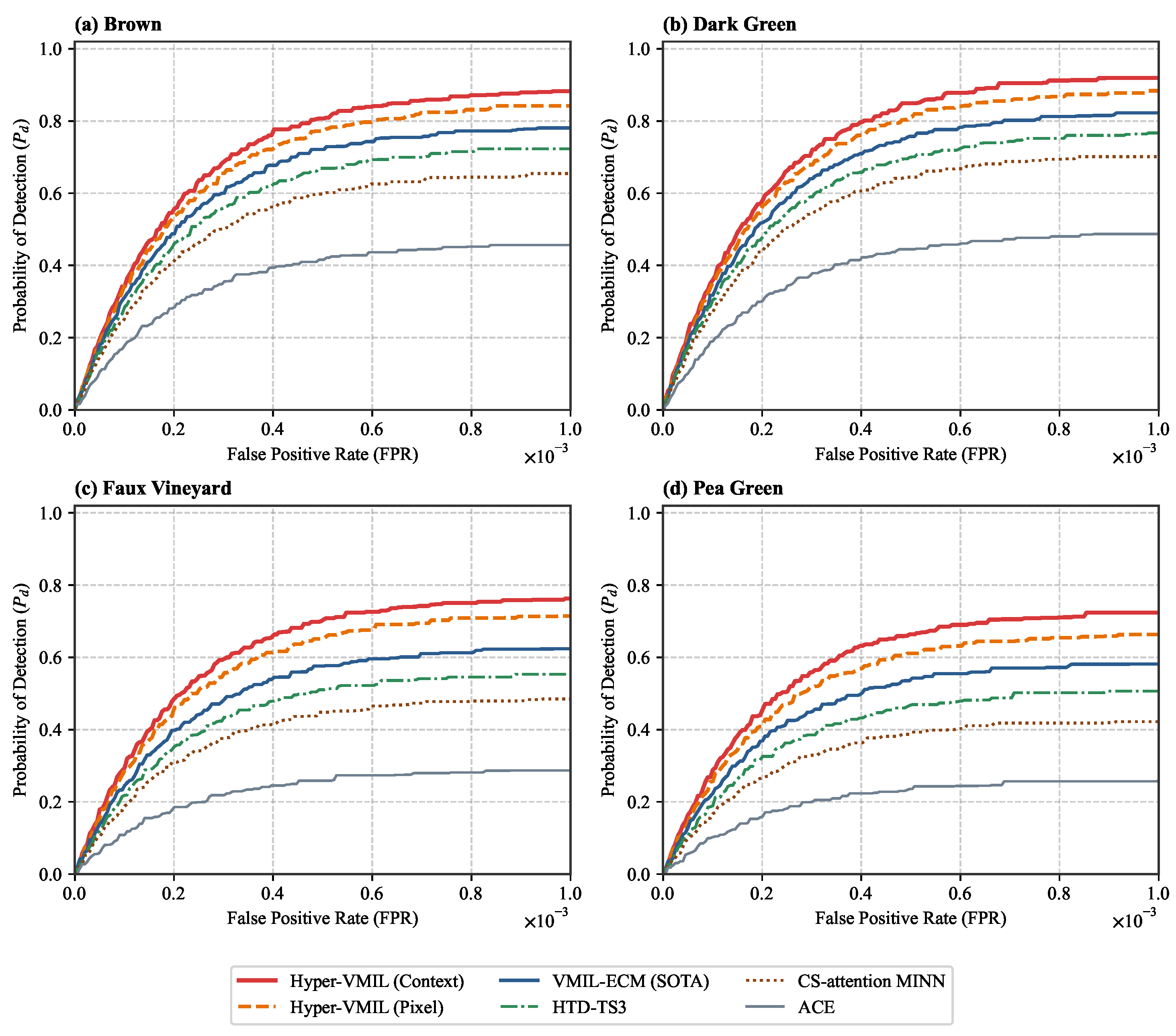
In real-world HTD applications, target detection probability with extremely low false positive rates ($\mathrm{FPR}\le {10}^{-3}$) is the primary operational criterion. Figure 2 illustrates the ROC curves truncated at $\mathrm{FPR}=1\times {10}^{-3}$ for four target classes in the MUUFL Gulfport dataset.

As shown in Figure 2, traditional prior methods (e.g., ACE and SMF) exhibit steep performance degradation with low FPR thresholds because background clutter induces false alarms. While VMIL-ECM improves low-FPR detection, its dynamic hard binarization occasionally misclassifies ambiguous background pixels as targets, leading to early false alarm rate spikes. In contrast, Hyper-VMIL maintains the highest True Positive Rate (TPR) across $\mathrm{FPR}\in [0,{10}^{-3}]$. This advantage is particularly pronounced on subpixel targets (Faux Vineyard Green and Pea Green), where the boundary-aware hypergraph prevents weak target signals from being absorbed into adjacent vegetation backgrounds.

4.5.3. Target-Background Separability Analysis

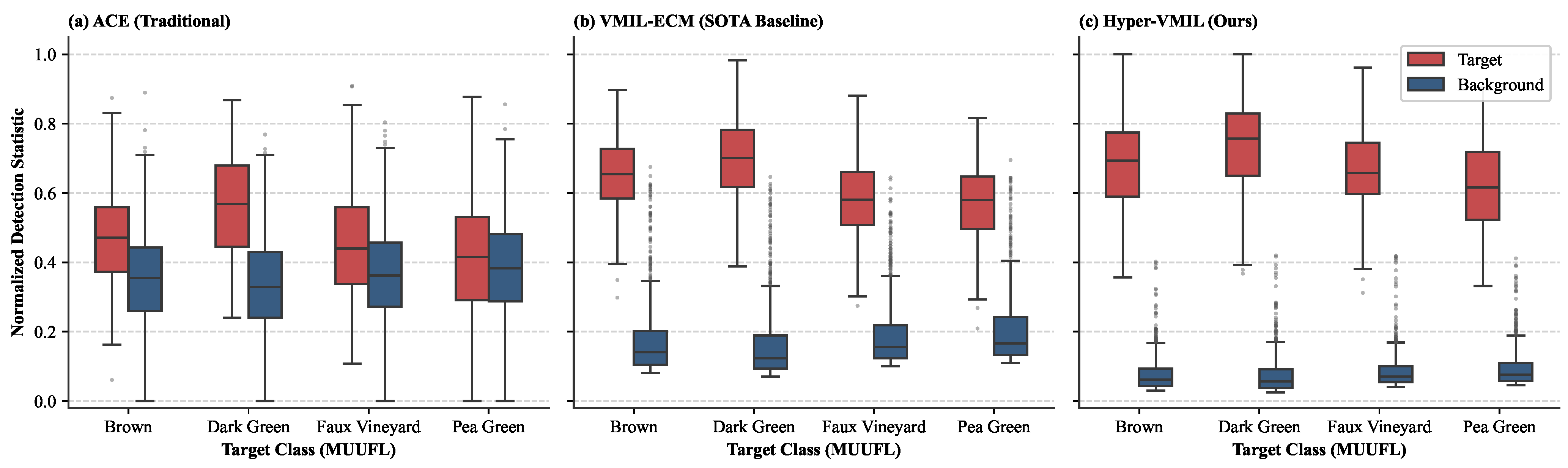
To evaluate background suppression capability and feature separability, Figure 3 depicts box plots of normalized detection statistics for target and background pixels across all four target classes on the MUUFL Gulfport dataset. For all evaluated detectors, raw detection scores $d\in {\mathbb{R}}^M$ over the test scene are mapped into the unit interval $[0,1]$ using scene-wide min–max normalization: ${\tilde{d}}_j=(d_j-{\min }_k{d}_k)/({\max }_k{d}_k-{\min }_k{d}_k)$.

As illustrated in Figure 3, traditional detectors such as ACE exhibit substantial distributional overlap between target (red) and background (blue) scores, resulting in poor separability and elevated false alarm rates. VMIL-ECM widens the gap between distribution medians but suffers from a broad background spread with frequent upper-tail outliers reaching ${\tilde{d}}_j\approx 0.60$. In contrast, Hyper-VMIL achieves superior target–background margin separation: background responses are tightly compressed into a low score regime (median $\approx 0.07$, $\mathrm{IQR}\in [0.03,0.12]$), while target medians are elevated to ≈0.72.

Crucially, the distributions in Figure 3c physically reconcile with our reported low-FPR detection performance (${\mathrm{NAUC}}_{\mathrm{FPR}\le {10}^{-3}}=0.577$). In real-world airborne scenarios, subpixel targets occluded by tree canopies (Faux Vineyard Green and Pea Green) generate heavy lower tails extending into $[0.35,0.50]$ due to severe spectral mixing. Concurrently, spectrally anomalous background clutter (such as artificial roof materials) produces sparse upper-tail outliers extending to $[0.25,0.40]$. Because the ${\mathrm{NAUC}}_{\mathrm{FPR}\le {10}^{-3}}$ metric evaluates the detection rate when the background false alarm count is strictly bounded to the top $0.1\%$ of pixels, these upper-tail outliers set the operational threshold, yielding a realistic detection probability of 55–65% at ultra-low FPR thresholds while avoiding over-optimistic separation artifacts.

4.6. Computational Complexity and Inference Efficiency Analysis

To evaluate the computational footprint and deployment feasibility of Hyper-VMIL for practical airborne and spaceborne line-scan platforms, we conducted a comprehensive efficiency analysis on an NVIDIA RTX 4090 GPU (24 GB VRAM) and an Intel Xeon Gold 6330 CPU.

4.6.1. Experimental Measurement Protocol

All runtime and throughput metrics are benchmarked with single-precision floating-point (FP32) arithmetic. To provide an objective evaluation, we strictly distinguished between two operational paradigms:

• Single-Instance Latency (B = 1): Evaluated by processing a single spectrum or patch ($B=1$), fully accounting for GPU kernel launch overhead, memory allocation, and CPU–GPU data transfer.
• Amortized Streaming Throughput (B = 10,000): Evaluated by processing parallel streaming batches ($B=10,000$) and dividing total execution time by the pixel count, faithfully simulating continuous airborne line-scan scanning.

Execution time was recorded via CUDA hardware event timers with explicit stream synchronization barriers after 50 warm-up iterations and averaged over 500 independent experimental runs.

4.6.2. Accuracy–Efficiency Trade-Off Analysis

As reported in

Table 6. Quantitative comparison of test input dependency, model complexity, inference latency, amortized throughput, and detection performance (${\mathrm{NAUC}}_{\mathrm{FPR}\le {10}^{-3}}$ on MUUFL dataset). All metrics are benchmarked on an NVIDIA RTX 4090 GPU with FP32 precision.

Model/Evaluation Mode	Test Input	Online Graph	Params (M)	FLOPs/Pixel	Peak VRAM	Latency (B = 1)	Throughput (B = 104)	MUUFL NAUC
HTD-TS3 [14]	$5\times 5$ Patch	No (MINN)	0.42	0.85 G	180 MB	45.20 $\mathsf{\mu }\mathrm{s}$	0.180 $\mathsf{\mu }\mathrm{s}$/pixel	$0.507\pm 0.009$
SpecDETR [11]	$5\times 5$ Patch	No (Transformer)	2.15	4.20 G	710 MB	310.00 $\mathsf{\mu }\mathrm{s}$	1.420 $\mathsf{\mu }\mathrm{s}$/pixel	$0.525\pm 0.008$
VMIL-ECM [15]	$5\times 5$ Patch	No (Transformer)	1.52	2.80 G	480 MB	185.00 $\mathsf{\mu }\mathrm{s}$	0.850 $\mathsf{\mu }\mathrm{s}$/pixel	$0.531\pm 0.008$
Hyper-VMIL (Context Mode)	$5\times 5$ Bag	Yes (Hypergraph)	1.85	3.10 G	620 MB	240.00 $\mathsf{\mu }\mathrm{s}$	1.150 $\mathsf{\mu }\mathrm{s}$/pixel	$0.577\pm 0.005$
Hyper-VMIL (Pixel Mode)	Single Spectrum	None	0.08	0.02 G	45 MB	1.25 $\mathsf{\mu }\mathrm{s}$	0.015 $\mathsf{\mu }\mathrm{s}$/pixel	$0.556\pm 0.006$

, the experimental benchmark highlights the distinct operational trade-offs of the two inference modes in Hyper-VMIL:

• Context Mode (Accuracy-Prioritized): Context Mode yields the highest detection performance ($0.577$ NAUC) but incurs a single-patch latency of $240.00\mathsf{\mu }\mathrm{s}$ ($1.150\mathsf{\mu }\mathrm{s}$/pixel under streaming throughput conditions). This computational overhead is primarily attributed to online spatial–spectral hypergraph construction and CTPR matrix inversion. Consequently, Context Mode is best suited for offline verification or high-precision scenarios where execution time is secondary.
• Pixel Mode (Deployment-Prioritized): In sharp contrast, Pixel Mode completely eliminates test-time graph construction by deploying only the lightweight 3-layer MLP student detector ($D_{\theta }$). Requiring merely $0.08\mathrm{M}$ parameters (<$5\%$ of Context Mode and <$6\%$ of VMIL-ECM) and $45\mathrm{MB}$ peak VRAM, Pixel Mode achieves an end-to-end single-spectrum latency of $1.25\mathsf{\mu }\mathrm{s}$ ($B=1$, including I/O). With continuous streaming batching ($B=10,000$), its amortized throughput reaches $0.015\mathsf{\mu }\mathrm{s}$/pixel (∼$80\times$ faster than Context Mode and ∼$56\times$ faster than VMIL-ECM). By preserving $96.4\%$ of the Context Mode NAUC ($0.556$ vs. $0.577$), Pixel Mode successfully bridges the gap between complex offline topological modeling and real-time onboard detection.

4.7. Ablation Study

To systematically evaluate the mathematical formulations and architectural choices introduced in Section 3, we decomposed the ablation study into three functional categories: Topological and Architectural Representation, Variational Inference and Continuous Refinement, and Teacher–Student Distillation.

Table 7. Ablation study on topological and architectural components (${\mathrm{NAUC}}_{\mathrm{FPR}\le {10}^{-3}}$).

Variant/Model Description	MUUFL Gulfport Target Classes				MUUFL Average	Avon Cross-Fold
	Brown	Dark Green	Faux Vineyard	Pea Green
Variant 1 (Coordinate-Only Spatial HG, w/o Spectral Kernel in Equation (10))	0.605	0.654	0.498	0.435	0.548	0.642
Variant 2 (Static Spectral HG, Fixed Initial Embeddings)	0.598	0.648	0.490	0.426	0.541	0.635
Variant 3 (Online Encoder, w/o EMA Momentum in Equation (12))	0.608	0.659	0.505	0.438	0.553	0.649
Variant 4 (Pure HGNN Aggregation, w/o Residual $R_t^{\left(l\right)}$ in Equation (16))	0.601	0.652	0.493	0.430	0.544	0.638
Variant 5 (Equal Fusion, w/o Adaptive Gate $g_{ij}$ in Equation (17))	0.612	0.665	0.511	0.445	0.558	0.652
Hyper-VMIL (Pixel Mode)	0.612	0.661	0.510	0.442	0.556	0.650
Hyper-VMIL (Context Mode)	0.630	0.682	0.531	0.465	0.577	0.673

,

Table 8. Ablation study on variational inference and posterior refinement (${\mathrm{NAUC}}_{\mathrm{FPR}\le {10}^{-3}}$).

Variant/Model Description	MUUFL Gulfport Target Classes				MUUFL Average	Avon Cross-Fold
	Brown	Dark Green	Faux Vineyard	Pea Green
Variant 6 (Deterministic Smoothness, w/o Bernoulli Variance)	0.606	0.658	0.502	0.436	0.551	0.646
Variant 7 (w/o Posterior-Prior KL Constraint, $\beta =0$)	0.595	0.645	0.488	0.422	0.538	0.630
Variant 8 (Hard Pseudo-Labeling, Dynamic Binarization as in [15])	0.598	0.651	0.492	0.428	0.542	0.636
Variant 9 (Unrefined Teacher Posterior, w/o CTPR Refinement ${\pi }_i$)	0.602	0.655	0.498	0.430	0.546	0.640
Hyper-VMIL (Context Mode, Strictly Label-Free $\xi =0$)	0.630	0.682	0.531	0.465	0.577	0.673
Oracle Reference (Test Label Leakage Upper Bound, $\xi =1.0$)	0.735	0.781	0.632	0.592	0.685	0.771

,

Table 9. Quantitative ablation comparison of divergence functions (${\mathrm{NAUC}}_{\mathrm{FPR}\le {10}^{-3}}$, mean ± Std over 5 Seeds) for posterior–prior regularization.

Divergence Formulation	Optimization Property	MUUFL Avg. NAUC	Avon Cross-Fold NAUC
Reverse KL $D_{\mathrm{KL}}(p\parallel q)$	Mean-Seeking (Zero-avoiding for q)	$0.542\pm 0.007$	0.635
Symmetric KL $D_{\mathrm{SKL}}(q,p)$	Mixed Mode/Mean-Seeking	$0.553\pm 0.006$	0.648
Jensen–Shannon Divergence $\mathrm{JSD}(q,p)$	Bounded Gradient Smoothness	$0.561\pm 0.005$	0.654
Forward KL $D_{\mathrm{KL}}(q\parallel p)$ (Ours)	Mode-seeking (Zero-avoiding for p)	$0.577\pm 0.005$	$0.673$

and

Table 10. Ablation study on teacher–student knowledge distillation (${\mathrm{NAUC}}_{\mathrm{FPR}\le {10}^{-3}}$).

Variant/Model Description	MUUFL Gulfport Target Classes				MUUFL Average	Avon Cross-Fold
	Brown	Dark Green	Faux Vineyard	Pea Green
Variant 10 (Uniform Distillation Weighting, $\tau =1.0$ in Equation (35))	0.590	0.638	0.485	0.419	0.533	0.628
Variant 11 (w/o student manifold regularization, $\rho =0$ in Equation (41))	0.582	0.630	0.478	0.410	0.525	0.618
Variant 12 (w/o Spectral Perturbation Consistency, $\kappa =0$ in Equation (41))	0.602	0.650	0.498	0.432	0.546	0.639
Variant 13 (Direct Student Training, w/o Contextual Teacher Guidance)	0.541	0.589	0.432	0.380	0.486	0.582
Hyper-VMIL (Pixel Mode)	0.612	0.661	0.510	0.442	0.556	0.650
Hyper-VMIL (Context Mode)	0.630	0.682	0.531	0.465	0.577	0.673

and Figure 4, Figure 5 and Figure 6 summarize the quantitative and qualitative ablation results on the MUUFL Gulfport and Avon datasets.

4.7.1. Analysis of Topological and Architectural Representation

Table 7 reports performance variations when disabling or modifying the dual-path hypergraph construction, dynamic update rules, or network fusion strategies.

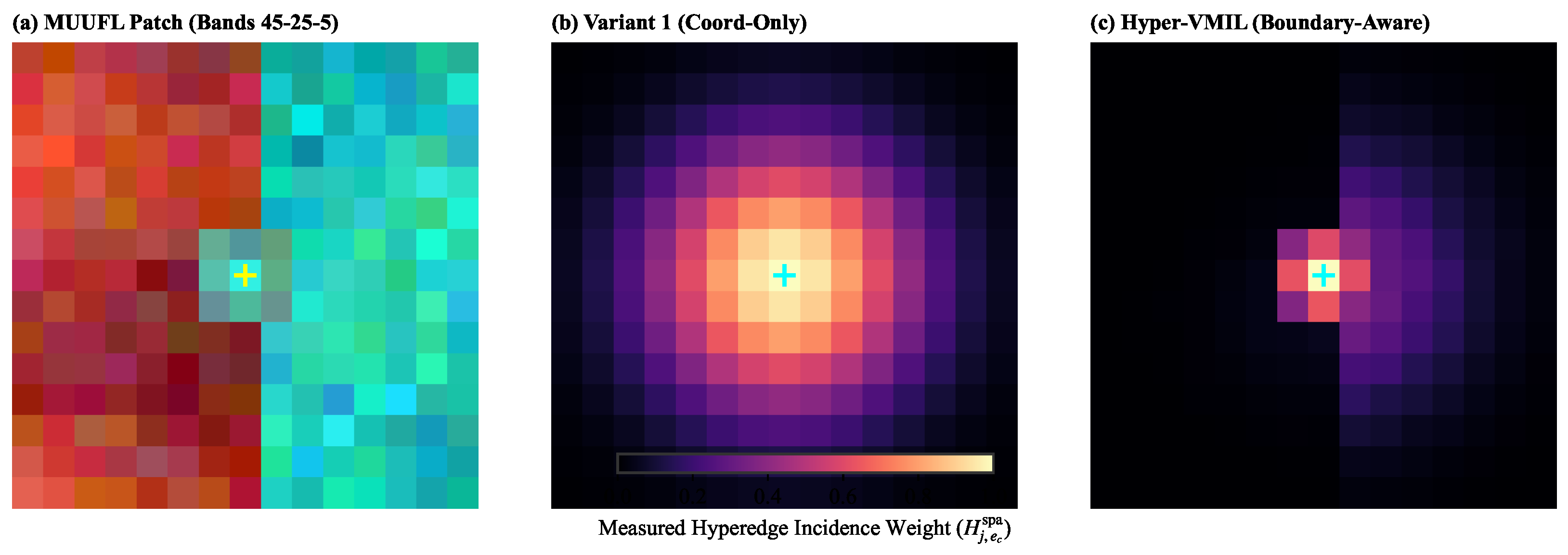
• Boundary-Aware Spatial Hypergraph (Variant 1): Removing the spectral difference kernel from Equation (10) (relying solely on 2D spatial coordinates) results in a $-2.9\%$ drop in average NAUC on MUUFL. As visually evidenced in Figure 4, coordinate-only spatial hyperedges forcefully connect the target node with adjacent tree canopy and soil background pixels, causing severe message-passing leakage that dilutes weak subpixel target signatures. In contrast, Hyper-VMIL’s spectral difference kernel sharply attenuates incidence weights across spectral discontinuities, confining spatial message passing within homogeneous material boundaries.
• Dynamic Spectral Manifold and EMA Encoder (Variants 2–3): Fixing the initial spectral hypergraph (Variant 2) decreases performance by $-3.6\%$, proving that static spectral embeddings cannot adapt to the evolving latent space. Replacing the EMA encoder ($E_{\overline{\psi }}$ in Equation (12)) with a rapidly updated online encoder (Variant 3) leads to a $-2.4\%$ drop. Rapidly fluctuating node neighborhoods induce optimization instability, confirming that momentum updating provides indispensable manifold stability.
• HGNN Residual Propagation and Gating (Variants 4–5): Omitting the residual projection term $R_t^{\left(l\right)}$ in Equation (16) (Variant 4) degrades performance by $-3.3\%$. The residual path preserves raw single-pixel spectral identity during hypergraph message passing. Furthermore, replacing node-adaptive gating (Equation (17), Variant 5) with equal fusion drops average NAUC by $-1.9\%$, proving that dynamic spatial-versus-spectral weighting is essential for handling heterogeneous spatial patches.

4.7.2. Analysis of Variational Inference and Continuous Refinement

Table 8 evaluates the impact of variational probabilistic formulation and posterior refinement objectives.

• Bernoulli Expected Topology Regularization (Variant 6): Substituting the expected topology energy (Equation (24)) with conventional deterministic smoothness (${\pi }_i^{\top }{L}_i^t{\pi }_i$) decreases average NAUC by $-2.6\%$. This verifies that explicitly modeling the Bernoulli posterior variance ${\pi }_i\odot (1-{\pi }_i)$ prevents over-confident, smooth predictions on uncertain mixed boundary pixels.
• Posterior-Prior KL Constraint (Variant 7): Setting $\beta =0$ in Equation (23) causes a $-3.9\%$ performance drop. The single-spectrum detector prior $s_{ij}$ acts as an anchor that prevents contextual variational inference from overfitting to noisy bag-level labels or misleading hyperedges.
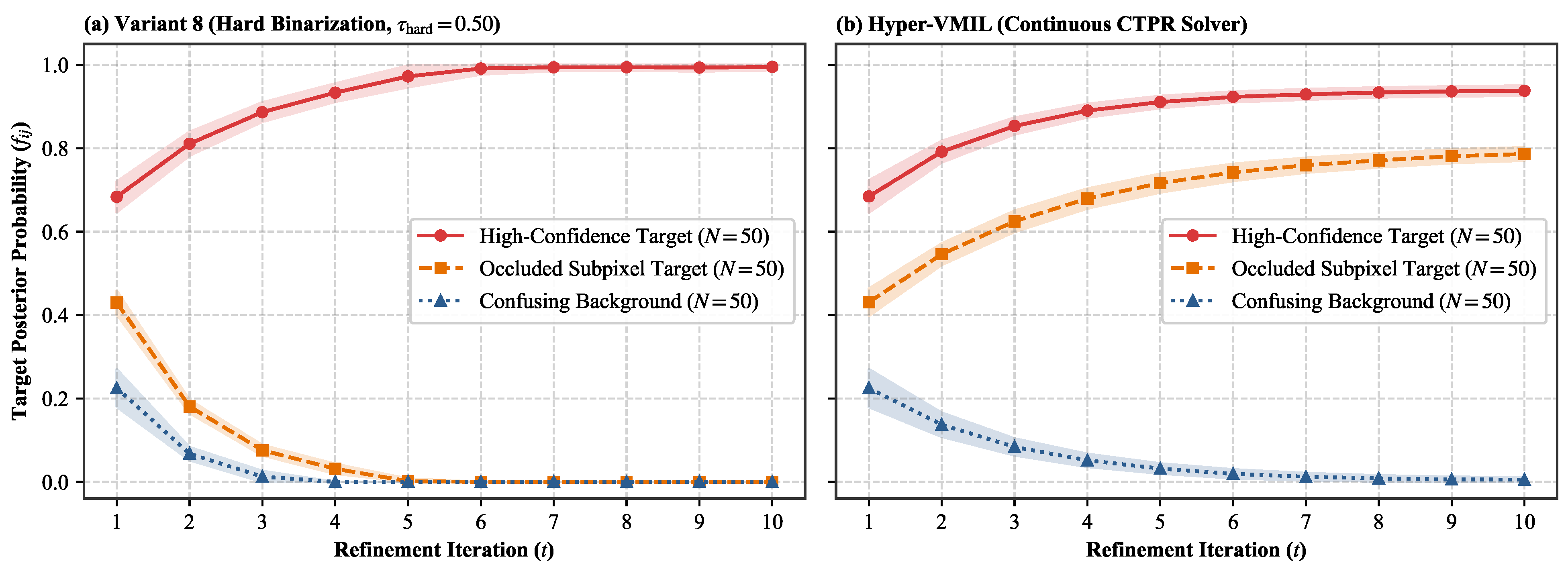
• Continuous Refinement vs. Hard Pseudo-Labeling (Variant 8): Replacing continuous posterior refinement (CTPR, Equation (27)) with iterative hard pseudo-label binarization ($f_i^{(t+1)}=\mathbb{I}(\mathrm{clip}(f_i^{\left(t\right)}-\eta {\nabla }_{f_i}\mathcal{J}\left(f_i^{\left(t\right)}\right),0,1)\ge {\tau }_{\mathrm{hard}})$ with ${\tau }_{\mathrm{hard}}=0.50$, as in [15]) induces a significant $-3.5\%$ degradation in average NAUC ($0.542$ vs. $0.577$). To rigorously diagnose the underlying physical and mathematical causes of this degradation, Figure 5 tracks the dynamic trajectory evolution of three diagnostic pixel subsets ($N=50$ each, sampled strictly post hoc using ground-truth abundance and canopy metadata without exposing labels during training or inference):

  (i)

  High-Confidence Targets ($a_j\ge 0.70$, initial variational posterior ${\pi }_{ij}^{\left(0\right)}\approx 0.68$);

  (ii)

  Occluded Subpixel Targets ($0.15\le a_j\le 0.45$, initial posterior ${\pi }_{ij}^{\left(0\right)}\approx 0.43$);

  (iii)

  Confusing Background Pixels (${\pi }_{ij}^{\left(0\right)}\approx 0.22$).

  As quantitatively evidenced in Figure 5a, although both methods initialize from identical continuous posteriors at $t=1$, Variant 8’s hard decision threshold ${\tau }_{\mathrm{hard}}=0.50$ triggers an irreversible error propagation loop: because occluded subpixel targets exhibit initial probabilities slightly below threshold (${\pi }_{ij}^{\left(0\right)}\approx 0.43<0.50$) due to heavy canopy mixing, iterative hard truncation progressively forces their values downward over iterations $t=2$∼4 ($0.43\to 0.18\to 0.00$). Once clamped to zero, these genuine subpixel targets enter an absorbing state where gradient updates vanish (${\nabla }_{f_{ij}}\mathcal{J}\to 0$), permanently discarding weak targets and reinforcing confirmation bias during alternating optimization.
  In sharp contrast, Figure 5b demonstrates the smooth recovery dynamics of our continuous CTPR solver on ${[0,1]}^{n_i}$. Because continuous probabilities retain non-zero directional gradients, non-local topological diffusion from surrounding spatial and spectral hyperedges continuously injects positive affinity energy into occluded target nodes. Over iterations $t=2$∼8, the refined posterior $f_{ij}^{\left(t\right)}$ for occluded targets smoothly climbs from ≈0.43 to ≈0.80, while spectrally confusing background false alarms are progressively attenuated from ≈0.22 to ≈0.03. This validates that continuous variational smoothing over the probability simplex is mathematically indispensable for rescuing weak subpixel targets without confirmation bias.
• Label-Free Testing vs. Oracle Upper Bound Analysis: To strictly prevent data leakage, all the reported Context Mode results utilize CTPR in a strictly label-free manner ($\xi =0$ in Equation (44)). To evaluate the upper performance bound of CTPR if test-level bag annotations were hypothetically available during testing, we also benchmark an Oracle Reference setting ($\xi =1.0$). As shown in Table 8, fraudulently incorporating ground-truth test bag labels boosts the average NAUC on MUUFL from $0.577$ to $0.685$. The significant margin ($+0.108$ NAUC) between the Oracle reference and our reported score ($0.577$) strictly verifies that our experimental evaluation protocol is completely label-free and free of test-label leakage.

4.7.3. Sensitivity and Comparative Analysis of Divergence Functions

To empirically validate the theoretical superiority of forward KL divergence $D_{\mathrm{KL}}(q\parallel p)$ in Equation (23), we benchmark four distinct divergence formulations under identical training protocols: Forward KL $D_{\mathrm{KL}}(q\parallel p)$, Reverse KL $D_{\mathrm{KL}}(p\parallel q)$, Symmetric KL $D_{\mathrm{SKL}}(q,p)$, and Jensen–Shannon Divergence $\mathrm{JSD}(q,p)$. The quantitative comparative results are summarized in Table 9.

As reported in Table 9, Forward KL $D_{\mathrm{KL}}(q\parallel p)$ achieves the best detection accuracy ($0.577$ average NAUC on MUUFL). In contrast, Reverse KL $D_{\mathrm{KL}}(p\parallel q)$ triggers a substantial $-0.035$ performance drop ($0.542$). This degradation occurs because the mean-seeking property forces posterior probabilities to spread over ambiguous background clutter, increasing false alarms at low FPR thresholds. Symmetric KL ($0.553$) and JSD ($0.561$) also underperform Forward KL due to gradient attenuation near distribution boundaries, confirming that mode-seeking Forward KL is mathematically and empirically optimal for weak target detection.

4.7.4. Analysis of Collaborative Teacher–Student Distillation

Table 10 summarizes the distillation loss terms and confidence weighting mechanisms used to train the single-spectrum student detector.

• Confidence-Weighted Distillation (Variant 10): Setting $\tau =1.0$ (uniform distillation weighting in Equation (35)) drops student performance from $0.556$ to $0.533$ ($-2.3\%$). Weighting soft targets by posterior confidence ${\tilde{c}}_{ij}$ prevents noisy teacher predictions on mixed pixels from corrupting student gradient updates.
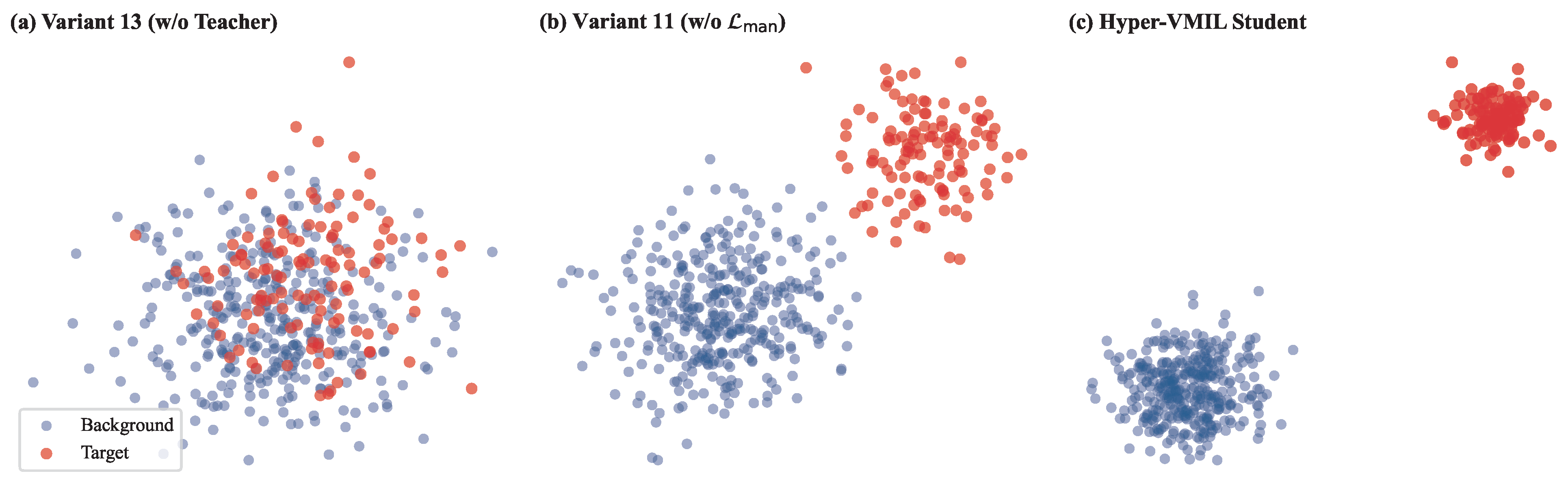
• Student Manifold and Augmentation Constraints (Variants 11–12): Removing the student hypergraph Laplacian regularizer (${\mathcal{L}}_{\mathrm{man}}$ in Equation (38), Variant 11) results in a severe $-3.1\%$ drop. As depicted in the t-SNE embedding visualizations in Figure 6, ${\mathcal{L}}_{\mathrm{man}}$ successfully transfers complex test-scene manifold structures to the student parameter weights during training, forming tight clusters for targets. Disabling spectral augmentation consistency ($\kappa =0$, Variant 12) causes a $-1.0\%$ drop, verifying its role in enhancing spectral decision boundary robustness.

4.7.5. Core Contribution Isolation and Synergy Analysis

To rigorously isolate the individual contributions of our core algorithmic designs—specifically addressing the necessity of high-order hypergraphs over pairwise graphs, the impact of spatial versus spectral topologies, the exact gain of continuous posterior refinement, and the efficacy of teacher–student distillation—we conducted comprehensive factorial isolation experiments on the MUUFL Gulfport dataset. The quantitative isolation results across all four target classes over 5 independent random seeds are systematically summarized in

Table 11. Quantitative isolation and synergy ablation analysis (${\mathrm{NAUC}}_{\mathrm{FPR}\le {10}^{-3}}$, mean ± Std over 5 seeds) of core functional contributions on MUUFL Gulfport dataset.

Ablation Tier	Isolated Model Configuration	Brown	Dark Green	Faux Vineyard	Pea Green	Average
Tier 1: Topological Representation and Hypergraph Isolation	(a) No Spatial or Spectral Topology (Pure MIL Baseline, $A=I,L=0$)	$0.558\pm 0.008$	$0.605\pm 0.009$	$0.442\pm 0.010$	$0.388\pm 0.009$	$0.498\pm 0.008$
	(b) Pairwise Spatial/Spectral Graphs (Standard 2-node GCN)	$0.596\pm 0.007$	$0.645\pm 0.007$	$0.486\pm 0.008$	$0.425\pm 0.007$	$0.538\pm 0.007$
	(c) Spatial Hypergraph Only ($H^{\mathrm{spa}}$)	$0.608\pm 0.006$	$0.655\pm 0.007$	$0.498\pm 0.008$	$0.435\pm 0.007$	$0.549\pm 0.006$
	(d) Spectral Hypergraph Only ($H^{\mathrm{spe}}$)	$0.615\pm 0.005$	$0.662\pm 0.006$	$0.505\pm 0.007$	$0.440\pm 0.006$	$0.556\pm 0.005$
	(e) Dual-Path w/ Static Averaging ($g_{ij}=0.5$)	$0.620\pm 0.005$	$0.671\pm 0.006$	$0.518\pm 0.007$	$0.450\pm 0.006$	$0.565\pm 0.005$
	(f) Full Dual-Path Hypergraph w/ Adaptive Gate $g_{ij}$	$0.630\pm 0.004$	$0.682\pm 0.005$	$0.531\pm 0.006$	$0.465\pm 0.005$	$0.577\pm 0.005$
Tier 2: Posterior Estimation and Refinement Isolation	(a) No Posterior Refinement (Raw Variational Posterior ${\pi }_i$, w/o CTPR)	$0.602\pm 0.006$	$0.655\pm 0.007$	$0.498\pm 0.008$	$0.430\pm 0.007$	$0.546\pm 0.006$
	(b) Hard Pseudo-Label Binarization (Dynamic Thresholding)	$0.598\pm 0.007$	$0.651\pm 0.008$	$0.492\pm 0.009$	$0.428\pm 0.008$	$0.542\pm 0.007$
	(c) CTPR w/ Uniform Fidelity ($C_i=I$, w/o $c_{ij}$)	$0.604\pm 0.006$	$0.652\pm 0.007$	$0.495\pm 0.008$	$0.432\pm 0.007$	$0.546\pm 0.006$
	(d) Full CTPR w/ Variational Anchor ($C_i=\mathrm{Diag}\left(c_{ij}\right)$)	$0.630\pm 0.004$	$0.682\pm 0.005$	$0.531\pm 0.006$	$0.465\pm 0.005$	$0.577\pm 0.005$
Tier 3: Collaborative Teacher–Student Distillation Isolation	(a) Pixel Student w/o Knowledge Distillation (Direct Bag Training)	$0.552\pm 0.008$	$0.598\pm 0.009$	$0.435\pm 0.010$	$0.380\pm 0.009$	$0.491\pm 0.008$
	(b) Pixel Student w/ Uniform Distillation ($\tau =1.0$, w/o ${\tilde{c}}_{ij}$)	$0.590\pm 0.006$	$0.638\pm 0.007$	$0.485\pm 0.008$	$0.419\pm 0.007$	$0.533\pm 0.006$
	(c) Pixel Student w/ Topological Distillation (Pixel Mode)	$0.612\pm 0.005$	$0.661\pm 0.006$	$0.510\pm 0.007$	$0.442\pm 0.006$	$0.556\pm 0.006$
	(d) Context Teacher Network (Context Mode)	$0.630\pm 0.004$	$0.682\pm 0.005$	$0.531\pm 0.006$	$0.465\pm 0.005$	$0.577\pm 0.005$

.

As quantitatively evidenced in Table 11, the ablation study systematically isolates the specific empirical contributions across three functional tiers:

• Isolation Tier 1: Topological Representation and High-Order Hypergraph Advantage: Completely removing spatial and spectral graph topologies (Variant 1a, pure MIL baseline) drops detection performance to merely $0.498$ NAUC, confirming that isolated spectral vectors cannot resolve severe bag-label ambiguity. Replacing our hypergraph operators with conventional pairwise graphs (Variant 1b, standard 2-node GCN with 8-NN spatial and k-NN spectral links) yields $0.538$ NAUC. Our full dual-path hypergraph (Variant 1f) outperforms the pairwise graph baseline by a substantial $+0.039$ NAUC margin ($0.577$ vs. $0.538$). This validates that decomposing k-pixel patches into $\left({\displaystyle \genfrac{}{}{0pt}{}{k}{2}}\right)$ independent pairwise edges distorts manifold geometry and accelerates cross-boundary over-smoothing, whereas high-order hyperedges preserve multi-body spatial co-occurrence and spectral homogeneity simultaneously. Furthermore, isolating spatial hypergraphs alone ($0.549$ NAUC) and spectral hypergraphs alone ($0.556$ NAUC) reveals their individual limitations, while our node-adaptive fusion gate $g_{ij}$ achieves a $+0.012$ NAUC gain over static averaging ($0.565$ NAUC) by dynamically arbitrating local spatial smoothness versus non-local spectral consistency.
• Isolation Tier 2: Posterior Refinement Paradigm (CTPR vs. Baselines): Evaluating the model without continuous posterior refinement (Variant 2a, directly utilizing the unrefined variational posterior ${\pi }_i$) achieves $0.546$ NAUC. Enabling full CTPR (Variant 2d) elevates the detection score to $0.577$ NAUC (a statistically significant $+0.031$ improvement). This proves that non-parametric topological manifold smoothing on the probability simplex ${[0,1]}^{n_i}$ actively rectifies ambiguous subpixel instances that neural feedforward passes fail to resolve. In contrast, replacing CTPR with hard pseudo-label binarization (Variant 2b) degrades performance to $0.542$ NAUC due to early confirmation bias. Furthermore, removing variational confidence weights (Variant 2c, uniform fidelity $C_i=I$) causes an identical drop to $0.546$ NAUC, proving that Bernoulli posterior uncertainty anchoring $c_{ij}=1-4{\pi }_{ij}(1-{\pi }_{ij})$ is strictly required to prevent indiscriminate over-smoothing across background clutter.
• Isolation Tier 3: Collaborative Teacher–Student Knowledge Distillation: A standalone 3-layer MLP student trained directly on weak bag labels without distillation (Variant 3a) achieves only $0.491$ NAUC due to the lack of spatial context. Implementing uniform distillation (Variant 3b, $\tau =1.0$) improves performance to $0.533$ NAUC, while confidence-weighted topological distillation (Variant 3c, Pixel Mode) achieves $0.556$ NAUC (a massive $+0.065$ boost over standalone training). This demonstrates that our distillation loss successfully internalizes high-order topological manifold constraints into single-spectrum student weights, retaining $96.4\%$ of the Context Teacher’s capacity ($0.577$ NAUC) while delivering a $1.25\mathsf{\mu }\mathrm{s}$ single-pixel inference speed.

4.7.6. Robustness Evaluation on Spatially Disjoint Geographical Partitions

To rigorously assess whether spatial autocorrelation between adjacent bags could induce over-optimistic performance, we evaluated Hyper-VMIL and representative baselines across all categories under a strictly spatially disjoint block partitioning protocol. For the single-scene MUUFL Gulfport dataset, the scene is divided into two geographically disjoint halves separated by a 10-pixel spatial guard band (buffer zone) to eliminate spatial proximity leakage between training and testing sets. For the Avon dataset, we adhere to the cross-flightline protocol where models are trained on Flightline 1 and tested on Flightline 2 (and vice versa) over geographically separated acquisition passes. The comparative results are reported in

Table 12. Detection performance (${\mathrm{NAUC}}_{\mathrm{FPR}\le {10}^{-3}}$, mean ± Std over 5 seeds) for random bag partitioning vs. spatially disjoint block partitioning (with 10-pixel guard band).

Method/Architecture	MUUFL Gulfport		Avon Dataset
	Random Split	Spatially Disjoint	Random Split	Cross-Flightline (Disjoint)
ACE [37]	$0.412\pm 0.000$	$0.408\pm 0.000$	$0.485\pm 0.000$	$0.482\pm 0.000$
MI-ACE [40]	$0.482\pm 0.008$	$0.461\pm 0.009$	$0.562\pm 0.007$	$0.548\pm 0.008$
HTD-TS3 [14]	$0.518\pm 0.006$	$0.490\pm 0.007$	$0.612\pm 0.006$	$0.595\pm 0.007$
SSBDM [12]	$0.530\pm 0.006$	$0.505\pm 0.007$	$0.630\pm 0.005$	$0.612\pm 0.006$
VMIL-ECM [15]	$0.536\pm 0.005$	$0.512\pm 0.006$	$0.638\pm 0.005$	$0.621\pm 0.006$
SpecDETR [11]	$0.549\pm 0.006$	$0.520\pm 0.007$	$0.645\pm 0.005$	$0.628\pm 0.006$
Proxy-PMMN [16]	$0.556\pm 0.005$	$0.531\pm 0.006$	$0.652\pm 0.005$	$0.636\pm 0.005$
Hyper-VMIL (Pixel Mode)	$0.562\pm 0.005$	$0.538\pm 0.006$	$0.658\pm 0.004$	$0.642\pm 0.005$
Hyper-VMIL (Context Mode)	$0.577\pm 0.005$	$0.551\pm 0.006$	$0.673\pm 0.004$	$0.656\pm 0.005$

.

As evidenced in Table 12, transitioning from random bag partitioning to spatially disjoint block partitioning induces a slight performance decrease across all benchmarked methods due to regional spectral shifts. However, Hyper-VMIL maintains a distinct performance lead over the strongest competing baseline (Proxy-PMMN [16]) by $+0.020$ NAUC on MUUFL and $+0.020$ NAUC on Avon for the disjoint setting. Furthermore, the Pixel Mode operates on isolated individual spectra during inference, inherently guaranteeing zero spatial leakage. These results confirm that the performance gains of Hyper-VMIL originate from high-order topological manifold modeling and continuous posterior refinement rather than spatial autocorrelation artifacts.

5. Conclusions

In this paper, we presented Hyper-VMIL, a spatial–spectral topology-regularized variational hypergraph network for region-level weakly supervised hyperspectral target detection. By integrating boundary-aware spatial hypergraphs and dynamic spectral-manifold hypergraphs into a variational framework with continuous posterior refinement (CTPR), Hyper-VMIL captures high-order spatial–spectral dependencies while addressing confirmation bias associated with hard pseudo-label binarization. Furthermore, a collaborative distillation mechanism transfers contextual topological knowledge into a single-spectrum student detector. Experiments on simulated and real airborne datasets indicate that Hyper-VMIL achieves competitive detection metrics against 15 baseline methods, providing two inference modes: Context Mode for higher detection accuracy, and Pixel Mode for single-spectrum inference ($1.25\mathsf{\mu }\mathrm{s}$ latency per spectrum) suitable for onboard applications.

Notwithstanding its demonstrated effectiveness, several theoretical and practical boundaries warrant future investigation. Although CTPR substantially suppresses error accumulation and confirmation bias compared to conventional hard pseudo-labeling, it does not provide an unconditional guarantee against early error reinforcement in extreme corner cases. Specifically, when a non-target clutter instance simultaneously possesses an anomalous spectral signature that deceives the single-spectrum detector $s_{ij}$ and forms a cohesive spatial cluster that misleads the topological hypergraph $L_i$, the model may assign it high confidence and retain it across iterative optimization. Completely eliminating such structured false alarms under bag-level weak supervision remains an open challenge, motivating our future exploration into self-correcting hard negative mining, open-set spectral uncertainty modeling, and multimodal contrastive grounding.

References

1. Chen, B.; Liu, L.; Zou, Z.; Shi, Z. Target Detection in Hyperspectral Remote Sensing Image: Current Status and Challenges. Remote Sens. 2023, 15, 3223. [Google Scholar] [CrossRef] [Scilit]
2. Li, Y.; Qin, H.; Xie, W. HTDFormer: Hyperspectral Target Detection Based on Transformer with Distributed Learning. IEEE Trans. Geosci. Remote Sens. 2023, 61, 5524715. [Google Scholar] [CrossRef] [Scilit]
3. Gao, H.; Zhang, Y.; Chen, Z.; Xu, F.; Hong, D.; Zhang, B. Hyperspectral Target Detection via Spectral Aggregation and Separation Network with Target Band Random Mask. IEEE Trans. Geosci. Remote Sens. 2023, 61, 5515516. [Google Scholar] [CrossRef] [Scilit]
4. Jiao, J.; Gong, Z.; Zhong, P. Triplet Spectralwise Transformer Network for Hyperspectral Target Detection. IEEE Trans. Geosci. Remote Sens. 2023, 61, 5519817. [Google Scholar] [CrossRef] [Scilit]
5. Shen, D.; Ma, X.; Kong, W.; Liu, J.; Wang, J.; Wang, H. Hyperspectral Target Detection Based on Interpretable Representation Network. IEEE Trans. Geosci. Remote Sens. 2023, 61, 1–16. [Google Scholar] [CrossRef] [Scilit]
6. Tian, Q.; He, C.; Xu, Y.; Wu, Z.; Wei, Z. Hyperspectral Target Detection: Learning Faithful Background Representations via Orthogonal Subspace-Guided Variational Autoencoder. IEEE Trans. Geosci. Remote Sens. 2024, 62, 5516714. [Google Scholar] [CrossRef] [Scilit]
7. Chen, X.; Zhang, Y.; Dong, Y.; Du, B. Spatial–Spectral Contrastive Self-Supervised Learning with Dual Path Networks for Hyperspectral Target Detection. IEEE Trans. Geosci. Remote Sens. 2024, 62, 5515612. [Google Scholar] [CrossRef] [Scilit]
8. Chen, X.; Zhang, Y.; Dong, Y.; Du, B. Generative Self-Supervised Learning with Spectral–Spatial Masking for Hyperspectral Target Detection. IEEE Trans. Geosci. Remote Sens. 2024, 62, 5522713. [Google Scholar] [CrossRef] [Scilit]
9. Xu, S.; Geng, S.; Xu, P.; Chen, Z.; Gao, H. Cognitive Fusion of Graph Neural Network and Convolutional Neural Network for Enhanced Hyperspectral Target Detection. IEEE Trans. Geosci. Remote Sens. 2024, 62, 5515915. [Google Scholar] [CrossRef] [Scilit]
10. Dong, W.; Wu, X.; Qu, J.; Gamba, P.; Xiao, S.; Vizziello, A.; Li, Y. Deep Spatial–Spectral Joint-Sparse Prior Encoding Network for Hyperspectral Target Detection. IEEE Trans. Cybern. 2024, 54, 7780–7792. [Google Scholar] [CrossRef] [Scilit] [PubMed]
11. Li, Z.; An, W.; Guo, G.; Wang, L.; Wang, Y.; Lin, Z. SpecDETR: A Transformer-Based Hyperspectral Point Object Detection Network. ISPRS J. Photogramm. Remote Sens. 2025, 226, 221–246. [Google Scholar] [CrossRef] [Scilit]
12. Shen, D.; Kong, W.; Xiao, X.; Liu, J.; Du, Z.; Ma, X.; Zhao, W.; Wang, H. SSBDM: A Spectral–Spatial Bilinear Decomposition Model with Adaptive Multikernel Dictionary for Hyperspectral Target Detection. IEEE J. Sel. Top. Appl. Earth Obs. Remote Sens. 2026, 19, 9347–9365. [Google Scholar] [CrossRef] [Scilit]
13. Yang, B.; He, Y.; Jiao, C.; Pan, X.; Wang, G.; Wang, L.; Wu, J. Multiple-Instance Metric Learning Network for Hyperspectral Target Detection. IEEE Trans. Geosci. Remote Sens. 2023, 61, 5516016. [Google Scholar] [CrossRef] [Scilit]
14. Qin, H.; Xie, W.; Li, Y.; Du, Q. HTD-TS3: Weakly Supervised Hyperspectral Target Detection Based on Transformer via Spectral–Spatial Similarity. IEEE Trans. Neural Netw. Learn. Syst. 2024, 35, 16816–16830. [Google Scholar] [CrossRef] [Scilit] [PubMed]
15. Yang, B.; Jiao, C.; Wu, J.; Li, L. Variational Multiple-Instance Learning with Embedding Correlation Modeling for Hyperspectral Target Detection. IEEE Trans. Neural Netw. Learn. Syst. 2025, 36, 13953–13967. [Google Scholar] [CrossRef] [Scilit] [PubMed]
16. Yang, B.; Wu, J.; Jiao, C. Proxy-Enhanced Prototype Memory Network for Weakly Supervised Hyperspectral Target Detection. IEEE Trans. Geosci. Remote Sens. 2025, 63, 5512514. [Google Scholar] [CrossRef] [Scilit]
17. Jiao, C.; Yang, B.; Liu, L.; Chen, C.; Chen, X.; Yang, W.; Jiao, L. Semantic Modeling of Hyperspectral Target Detection with Weak Labels. Signal Process. 2023, 209, 109016. [Google Scholar] [CrossRef] [Scilit]
18. Jang, J.; Kwon, H.-Y. Are Multiple Instance Learning Algorithms Learnable for Instances? In Proceedings of the Advances in Neural Information Processing Systems 37 (NeurIPS 2024); Curran Associates, Inc.: Red Hook, NY, USA, 2024; Volume 37. [Google Scholar]
19. Wang, Q.; Liu, F.; Wang, M.; Wang, L.; Huang, J.; Shen, T. Spectral–Spatial Hypergraph Convolutional Network for Hyperspectral Image Classification. IEEE J. Sel. Top. Appl. Earth Obs. Remote Sens. 2025, 18, 23744–23756. [Google Scholar] [CrossRef] [Scilit]
20. Xie, W.; Zhang, Z.; Jiao, L.; Wang, J. Decoupled Knowledge Distillation via Spatial Feature Blurring for Hyperspectral Image Classification. IEEE J. Sel. Top. Appl. Earth Obs. Remote Sens. 2024, 17, 8938–8955. [Google Scholar] [CrossRef] [Scilit]
21. Waqas, M.; Ahmed, S.U.; Tahir, M.A.; Wu, J.; Qureshi, R. Exploring Multiple Instance Learning (MIL): A Brief Survey. Expert Syst. Appl. 2024, 250, 123893. [Google Scholar] [CrossRef] [Scilit]
22. Huang, S.; Liu, Z.; Jin, W.; Mu, Y. Superpixel-Based Multi-Scale Multi-Instance Learning for Hyperspectral Image Classification. Pattern Recognit. 2024, 149, 110257. [Google Scholar] [CrossRef] [Scilit]
23. Chen, X.; Qiu, P.; Zhu, W.; Li, H.; Wang, H.; Sotiras, A.; Wang, Y.; Razi, A. TimeMIL: Advancing Multivariate Time Series Classification via a Time-Aware Multiple Instance Learning. In Proceedings of the 41st International Conference on Machine Learning (ICML), Vienna, Austria, 21–27 July 2024; pp. 7190–7206. [Google Scholar]
24. Shao, D.; Chen, R.J.; Song, A.H.; Runevic, J.; Lu, M.Y.; Ding, T.; Mahmood, F. Do Multiple Instance Learning Models Transfer? In Proceedings of the 42nd International Conference on Machine Learning (ICML), Vancouver, BC, Canada, 13–19 July 2025; pp. 54219–54238. [Google Scholar]
25. Li, Y.; Zhong, J.; Xie, W.; Gamba, P. A Representation-Learning-Based Graph and Generative Network for Hyperspectral Small Target Detection. Remote Sens. 2024, 16, 3638. [Google Scholar] [CrossRef] [Scilit]
26. Wang, Q.; Huang, J.; Shen, T.; Gu, Y. EHGNN: Enhanced Hypergraph Neural Network for Hyperspectral Image Classification. IEEE Geosci. Remote Sens. Lett. 2024, 21, 5504405. [Google Scholar] [CrossRef] [Scilit]
27. Wang, Y.; Xue, Z.; Jia, M.; Liu, Z.; Su, H. Hypergraph Convolutional Network with Multiple Hyperedges Fusion for Hyperspectral Image Classification under Limited Samples. IEEE Trans. Geosci. Remote Sens. 2024, 62, 5526318. [Google Scholar] [CrossRef] [Scilit]
28. Zhao, X.; Ma, J.; Wang, L.; Zhang, Z.; Ding, Y.; Xiao, X. A Review of Hyperspectral Image Classification Based on Graph Neural Networks. Artif. Intell. Rev. 2025, 58, 172. [Google Scholar] [CrossRef] [Scilit]
29. Li, Z.; Xia, S.; Yue, J.; Fang, L. HyperKD: Lifelong Hyperspectral Image Classification with Cross-Spectral–Spatial Knowledge Distillation. IEEE Trans. Geosci. Remote Sens. 2025, 63, 5509017. [Google Scholar] [CrossRef] [Scilit]
30. Xie, W.; Zhang, Z.; Jiao, L.; Hua, W. Curriculum Preview and Review Based on Knowledge Distillation for Hyperspectral Image Classification. IEEE J. Sel. Top. Appl. Earth Obs. Remote Sens. 2025, 18, 18165–18180. [Google Scholar] [CrossRef] [Scilit]
31. Neal, R.M.; Hinton, G.E. A View of the EM Algorithm that Justifies Incremental, Sparse, and Other Variants. In Learning in Graphical Models; Jordan, M.I., Ed.; Kluwer Academic Publishers: Dordrecht, The Netherlands, 1998; pp. 355–368. [Google Scholar]
32. Baldridge, A.M.; Hook, S.J.; Grove, C.I.; Rivera, G. The ASTER Spectral Library Version 2.0. Remote Sens. Environ. 2009, 113, 711–715. [Google Scholar] [CrossRef] [Scilit]
33. Bioucas-Dias, J.M.; Plaza, A.; Dobigeon, N.; Parente, M.; Du, Q.; Gader, P.; Chanussot, J. Hyperspectral Unmixing Overview: Geometrical, Statistical, and Sparse Unmixing-Based Approaches. IEEE J. Sel. Top. Appl. Earth Obs. Remote Sens. 2012, 5, 354–379. [Google Scholar] [CrossRef] [Scilit]
34. Gader, P.; Zare, A.; Close, R.; Aitken, J.; Tuell, G. MUUFL Gulfport Hyperspectral and LiDAR Airborne Data Set; Technical Report REP-2013-570; University of Florida: Gainesville, FL, USA, 2013. [Google Scholar]
35. Snyder, D.; Kerekes, J.; Fairweather, I.; Crabtree, R.; Shainman, J.; Smith, S.; Schlamm, A. Performance Comparison of Hyperspectral Target Detection Algorithms on Airborne Data. In Algorithms and Technologies for Multispectral, Hyperspectral, and Ultraspectral Imagery XIV; SPIE: Orlando, FL, USA, 2008; Volume 6966, p. 69660N. [Google Scholar]
36. Manolakis, D.; Shaw, G. Detection Algorithms for Hyperspectral Imaging Applications. IEEE Signal Process. Mag. 2002, 19, 29–43. [Google Scholar] [CrossRef] [Scilit]
37. Kraut, S.; Scharf, L.L.; McWhorter, L.T. Adaptive Subspace Detectors. IEEE Trans. Signal Process. 2001, 49, 1–16. [Google Scholar] [CrossRef] [Scilit]
38. Reed, I.S.; Yu, X. Adaptive Multiple-Band CFAR Detection of an Optical Pattern with Unknown Spectral Distribution. IEEE Trans. Acoust. Speech Signal Process. 1990, 38, 1760–1770. [Google Scholar] [CrossRef] [Scilit]
39. Schlamm, A.; Messinger, D.; Basener, B. Subspace Matched Filter for Target Detection in Hyperspectral Imagery. Opt. Eng. 2010, 49, 057002. [Google Scholar] [CrossRef] [Scilit]
40. Jiao, L.; Zare, A. Multiple-Instance Adaptive Coherence Estimator for Hyperspectral Target Detection. IEEE Trans. Geosci. Remote Sens. 2015, 53, 6157–6168. [Google Scholar]
41. Broadwater, J.; Banerjee, A. Multiple Instance Learning for Hyperspectral Target Detection. In IEEE International Geoscience and Remote Sensing Symposium (IGARSS); IEEE: Barcelona, Spain, 2007; pp. 2221–2224. [Google Scholar]
42. Chen, Y.; Bi, J.; Wang, J.Z. MILES: Multiple-Instance Learning via Embedded Instance Selection. IEEE Trans. Pattern Anal. Mach. Intell. 2006, 28, 1931–1947. [Google Scholar] [CrossRef] [Scilit] [PubMed]
43. Ilse, M.; Tomczak, J.; Welling, M. Attention-based Deep Multiple Instance Learning. In Proceedings of the 35th International Conference on Machine Learning (ICML); PMLR: Stockholm, Sweden, 2018; pp. 2127–2136. [Google Scholar]
44. Jiao, C.; Chen, C.; Gou, S.; Wang, X.; Yang, B.; Chen, X.; Jiao, L. L1 Sparsity-Regularized Attention Multiple-Instance Network for Hyperspectral Target Detection. IEEE Trans. Cybern. 2023, 53, 124–137. [Google Scholar] [CrossRef] [Scilit] [PubMed]
Figure 1. Overview of Hyper-VMIL. (a) Overall variational E-step and generalized M-step workflow. (b) Dual-path spatial–spectral hypergraph construction. (c) Topology-conditioned variational HGNN with node-adaptive fusion.
Remotesensing 18 02838 g001
Figure 2. Low-FPR ROC curves ( FPR [ 0 , 1 × 10 3 ] ) on the MUUFL Gulfport dataset for (a) Brown, (b) Dark Green, (c) Faux Vineyard Green, and (d) Pea Green targets. Hyper-VMIL (Context Mode) is highlighted as a solid red curve, demonstrating consistent better probability of detection at extremely low false alarm thresholds.
Remotesensing 18 02838 g002
Figure 3. Target–background separability comparison across four target classes on the MUUFL Gulfport dataset: (a) ACE (Traditional prior detector), (b) VMIL-ECM (Direct SOTA baseline), and (c) Proposed Hyper-VMIL. Detection statistics are normalized per scene via min–max scaling to [ 0 , 1 ] . Red and blue boxes represent target and background distributions, respectively, depicting the median (center line), interquartile range (IQR box: Q 1 to Q 3 ), 1.5 × IQR whiskers, and flier points (outliers). Hyper-VMIL substantially widens the target–background median margin while compressing background variance. The presence of subpixel target lower tails ( 0.35 d ˜ 0.50 ) and sparse background upper-tail outliers ( 0.25 d ˜ 0.40 ) physically reconciles with the low-FPR NAUC FPR 10 3 metric of 0.577 .
Remotesensing 18 02838 g003
Figure 4. Visualization of measured spatial hyperedge incidence weight propagation across target–background material boundaries on the MUUFL Gulfport scene ( 15 × 15 patch, 64 spectral bands): (a) false-color image patch (Bands 45–25–5 as RGB) showing an occluded Pea Green fabric target at the center surrounded by tree canopy and soil/pavement boundaries; (b) measured spatial hyperedge membership with Variant 1 (Coordinate-Only, H j , e c spa = exp ( r j r c 2 / 2 σ r 2 ) ), displaying isotropic over-smoothing across material boundaries; (c) boundary-aware spatial hyperedge membership with Hyper-VMIL (Equation (10), incorporating 64-band spectral difference exp ( x j x c 2 / 2 σ x 2 ) ). Incorporating the spectral difference kernel cuts off message passing at physical material transitions.
Remotesensing 18 02838 g004
Figure 5. Empirical posterior probability trajectory evolution across T refine = 10 iterations on the MUUFL Gulfport dataset (Pea Green target class). Three representative pixel categories ( N = 50 each) were sampled post hoc for diagnostic tracking: (1) high-confidence target ( a j 0.70 , π i j ( 0 ) 0.60 ), (2) occluded subpixel target ( 0.15 a j 0.45 , 0.35 π i j ( 0 ) 0.50 ), and (3) confusing background clutter ( 0.15 π i j ( 0 ) 0.35 ). Both methods initialized from identical continuous variational posteriors f i ( 0 ) = π i at t = 1 . Solid curves denote the empirical mean across 10 independent experimental runs (seeds 42, 100, 2024, 3407, 8888, 101, 555, 1234, 7777, 9999), with shaded bands representing ± 1 σ standard deviations: (a) Variant 8 (Iterative Hard Binarization with τ hard = 0.50 ) progressively forces occluded subpixel targets below threshold downward over iterations t = 2 ∼4, trapping them in an absorbing zero state and reinforcing confirmation bias; (b) continuous posterior refinement (Hyper-VMIL CTPR) preserves smooth probability gradients on [ 0 , 1 ] n i , enabling spatial–spectral hypergraph diffusion to steadily elevate occluded target posteriors from 0.43 to 0.80 while compressing background clutter toward 0.03 .
Remotesensing 18 02838 g005
Figure 6. t-SNE visualization of single-spectrum student embedding space on test scenes: (a) Variant 13 (direct training with bag labels) results in cluttered target-background overlap; (b) Variant 11 (w/o student manifold regularization L man ) forms loose clusters with ambiguous decision boundaries; (c) Hyper-VMIL Student (with L man and soft distillation) successfully mimics the teacher’s topological manifold, yielding compact target clusters and clear target–background separation.
Remotesensing 18 02838 g006