HNGT-Net: Hard-Negative Guided Topology Transfer for Lightweight Hyperspectral Small-Target Detection

Highlights

What are the main findings?

• HNGT-Net transfers local–global spectral–spatial topology through node, edge, and graph-Laplacian consistency.
• SG-HNS synthesizes hard negatives from normal samples and, together with responsemargin separation, yields an average AUC of 0.9953 across five benchmarks.

What are the implications of the main findings?

• Explicit hard-negative guidance improves small-target discrimination when training is restricted to normal hyperspectral samples.
• The 10.5-fold student-side parameter compression and compact teacher–student stack support resource-constrained remote sensing platforms and edge deployment.

Abstract

Detecting small anomalous targets in hyperspectral imagery is challenging when neither target spectra nor spatial morphologies are known, because most unsupervised detectors still encode implicit assumptions about background statistics or target structures and therefore generalize poorly to genuinely unknown threats. This paper introduces the Hard-Negative-Guided Topology Transfer Network (HNGT-Net), a lightweight teacher–student framework that addresses this problem from two perspectives. On the representation side, a similarity graph coupling spatial adjacency with feature-space nearest neighbors characterizes the spectral–spatial topology of normal backgrounds, and a three-level consistency objective over node embeddings, structural relations, and graph-Laplacian responses transfers this topology from a frozen teacher to a compact student. On the discrimination side, hard negatives are synthesized directly on pure normal pixels through sparsity-gated projected gradient perturbation, while a response-margin constraint forces the student to score such negatives above normal samples and mitigates distribution overfitting. Experiments on four public benchmark scenes and one Salinas-derived synthetic dataset show that HNGT-Net achieves an average AUC of 0.9953 with the smallest variance among all competitors. The student branch provides 10.5-fold parameter compression relative to the teacher, while the complete teacher–student stack remains compact, supporting resource-constrained remote sensing deployment.

1. Introduction

Among the most demanding problems in hyperspectral remote sensing is unsupervised hyperspectral anomaly detection (HAD), whose objective is to localize spectrally unusual targets without access to any prior target labels or reference spectra. Precisely because it dispenses with such prior knowledge, HAD has become indispensable in safety-critical applications such as environmental monitoring and resource exploration, where the signatures of potential threats cannot be anticipated in advance. This label-free property, however, should not be confused with assumption-free modeling. A careful inspection of prevailing unsupervised paradigms reveals that virtually all of them embed implicit hypotheses about the feature distributions of the background, the targets, or both; consequently, their generalization remains conditional on these modeling assumptions, and their generalization to genuinely unknown, small-target threats remains inherently limited. As Earth-observation missions increasingly demand the discovery of ever smaller and spectrally subtler anomalies under complex sensing conditions, these hidden assumptions turn from a theoretical caveat into a practical bottleneck, prompting a critical reassessment of the methodological foundations of the field.

A systematic review of deep learning-based hyperspectral anomaly detection provides a consolidated account of the field’s methodological development and persistent open challenges [1]. Alongside these developments, recent Remote Sensing studies have advanced the field along several complementary directions: the fractional Fourier transform-based tensor RX extends the RX statistic into the fractional domain while preserving spatial–spectral structure [2]; spatial–spectral union dictionary representation with improved saliency weighting strengthens background suppression [3]; fast collaborative representation with extended multi-attribute profiles reduces detection time without sacrificing accuracy [4]; and self-attention-aided deep unfolding converts tensor representation optimization into an interpretable trainable network [5]. Efficiency-oriented designs have likewise emerged, exemplified by a lightweight variational joint discrimination network that enables cross-image detection after a single training pass [6]. In the wider remote sensing detection literature, three obstacles central to this work have also been addressed separately: hard negative mining directs learning toward the most confusable background samples [7]; dynamic gradient adjustment rebalances easy and hard as well as positive and negative examples under severe sample imbalance [8]; and dedicated architectures improve small-target detection under complex backgrounds [9], while the spectrum difference enhanced network reports reduced model complexity for hyperspectral anomaly detection [10]. Nevertheless, these advances remain fragmented: hard negative construction, extreme background–anomaly imbalance, and small-target discriminability have rarely been treated jointly, and they have not been reconciled with deployment efficiency when supervision is strictly confined to normal samples.

To substantiate this argument, the literature is revisited through four complementary lenses: probabilistic background modeling, representation-driven reconstruction, low-rank and sparsity priors, and deep feature learning. For each lens, we focus on its underlying premise, subsequent development, and the limitation that remains under genuinely unknown small-target conditions.

The first methodological route models the background through explicit probability distributions. Statistical detectors form the earliest and most thoroughly investigated branch of HAD. Operating within the generalized likelihood ratio test (GLRT) framework, they first fit a probabilistic model to the background and then flag each test pixel as anomalous in proportion to its deviation from the estimated background statistics. The archetype of this lineage is the Reed–Xiaoli detector (RX), which assumes that background pixels obey a multivariate Gaussian distribution and adopts the Mahalanobis distance as the anomaly measure [11]. The elegance of this closed-form solution is offset by the fragility of the global Gaussian hypothesis in complex scenes, where background non-stationarity, nonlinear spectral mixing, and spatial heterogeneity are the norm rather than the exception. A rich family of RX variants has consequently emerged: the global RX (GRX) and local RX (LRX) [12] adapt the formulation to global and local background statistics, respectively; the kernel RX (KRX) [13] embeds the data in a higher-dimensional feature space so as to capture nonlinear spectral structures; the weighted RX (WRX) [14] applies per-pixel weighting to suppress contamination of the background estimate by anomalous pixels; and the segmented RX (RXSD) [15] divides the scene into homogeneous sub-regions to attenuate within-class variability. More recent efforts include the dual-window coupled modeling approach (DUWC) [16], which incorporates endmember learning into the statistical framework for enhanced discriminability, and the Deep-RX detector [17], which couples the classical formulation with deep generative constraints to better accommodate complex backgrounds. In parallel, Zhao et al. [18] introduced in Remote Sensing global and local real-time detectors that exploit the Woodbury matrix identity for causal pixel-by-pixel processing, markedly alleviating the computational burden of batch-mode statistical detectors without sacrificing accuracy. On the theoretical side, Feng et al. [19] proved the asymptotic equivalence of the Rao test, Wald test, and GLRT under the replacement model in hyperspectral imaging, thereby providing a unified justification for the family of RX-like detectors; yet Vincent et al. [20] further showed that, even under this more general replacement model, in which an anomaly substitutes for the background rather than being additively superimposed, the resulting detectors remain structurally bound to the presumed background covariance. Taken together, these detectors provide label-free inference but remain conditional on a prescribed background model, since their performance rests on the prior belief that the background conforms to a prescribed mathematical model. Against unknown small-scale threats, they are additionally sensitive to the covariance estimation window and the decision threshold, whose calibration typically requires laborious tuning guided by domain knowledge.

A second methodological route reconstructs background pixels through collaborative representations. Collaborative representation departs from explicit probabilistic modeling and instead rests on a discriminative premise: a background pixel can be faithfully reconstructed as a linear combination of its neighboring samples, whereas a spectrally distinct anomaly cannot be faithfully represented by any background dictionary, so that the reconstruction residual naturally serves as the anomaly score. This idea was crystallized in the collaborative representation-based detection (CRD) algorithm [21], which casts background suppression as a collaborative sparse coding problem. Because solving large-scale representation problems can be computationally prohibitive, much of the follow-up work has targeted efficiency and numerical stability: the recursive collaborative representation detector (RCRD) [22] exploits matrix inversion update strategies to accelerate the iterative solution process, and the ensemble and random collaborative representation detector (ERCRD) [23] improves robustness by randomly sub-sampling the background dictionary. Within the Remote Sensing domain, Hupel and Stütz [24] systematically benchmarked the classical RX, LRX, and CRD detectors for near real-time camouflage detection in multispectral imagery, reporting that all targets could be successfully detected with AUC greater than 0.9 and that vegetation index enhancement further bolsters detection robustness across diverse target types. A complementary stream of research strengthens spatial–spectral characterization and background suppression by incorporating auxiliary techniques: the spectral–spatial-enhanced low-rank collaborative representation (SSELRCR) method [25] couples collaborative representation with low-rank tensor decomposition to exploit the intrinsic multidimensional structure of hyperspectral data; He et al. [26] enhanced a recursive RX pipeline in Remote Sensing by introducing extended multi-attribute profiles, thereby allowing multiscale morphological context to inform background estimation in complex heterogeneous scenes; and the extended multi-attribute profile-based fast collaborative representation algorithm (EMAPKCRD) [4] likewise employs morphological attribute profiles to enrich the spatial descriptors available for background modeling. In addition, Wang et al. [27] formulated a self-weighted variant in which band importance and the background dictionary are learned jointly, thereby reducing interference from noisy or uninformative bands during reconstruction. Despite this continual refinement of dictionary construction and representation strategies, nearly all of these methods depend on sliding dual-window architectures for local background modeling, whose overhead is prohibitive for real-time processing at the edge; their accuracy is likewise dictated by the inner and outer window scales, which must be calibrated empirically with prior knowledge of anomaly spatial structures. These methods therefore remain strongly dependent on scene- and model-specific priors, and their generalization capability against unknown small-scale novel threats remains insufficient.

A third methodological route separates targets from backgrounds using low-rank and sparsity priors. This family achieves target–background separation by exploiting two complementary structural priors: the background spectra reside approximately in a low-rank subspace, whereas anomalous pixels are sparse. Its foundation is Robust Principal Component Analysis (RPCA) [28], which splits the hyperspectral data cube into a low-rank background matrix and a sparse anomaly matrix through convex relaxation. Theoretical elegance notwithstanding, the nuclear norm adopted by RPCA shrinks all singular values with equal strength, thereby penalizing minor and major spectral components indiscriminately and inadvertently erasing salient background information. To remedy this, weighted tensor Schatten p-norm minimization was introduced to impose milder penalties on dominant singular values, giving rise to Enhanced Tensor Robust Principal Component Analysis (ETRPCA) [29], which further refines background purification accuracy through tensor singular value decomposition. Along a complementary direction, Low-Rank and Sparse Matrix Decomposition (LSMAD) [30] and its extensions embed Mahalanobis distance metrics into the decomposition pipeline, so that the recovered low-rank background simultaneously supports statistical parameter estimation for joint background modeling and anomaly discrimination. More recently, with Saliency-Guided Sparse Low-Rank (SSLR), [31] coupled a three-dimensional tensor nuclear norm with pixel-level saliency weighting, allowing spectrally distinctive pixels to receive stronger emphasis while angular-distance constraints are preserved. Efficiency has also received considerable attention: the Iterative Multiple Random Compressed Sampling method based on Go-Decomposition (IMRCSGD) [32] adopts randomized sampling strategies to curb algorithmic complexity, and, targeting the computational demands of spectral decomposition on remote sensing platforms, Xue et al. [33] implemented a GPU-accelerated detection pipeline in Remote Sensing for airborne push-broom sensors, showing that hardware-level parallelization can substantially reduce the runtime burden of hyperspectral anomaly screening while preserving detection fidelity. Nevertheless, this family shares two structural weaknesses: the low-rank regularization tends to over-smooth faint, weakly energetic small targets by treating them as noise during reconstruction, destroying critical anomaly signatures; and the core operators hinge on large-scale singular value decomposition, whose computational cost renders real-time deployment under extreme sensing conditions impractical.

The fourth methodological route learns background representations through deep reconstruction networks. Fueled by their exceptional capacity for nonlinear feature representation, deep networks have recently risen to prominence in HAD and have spawned a broad spectrum of architectural innovations. The Multiscale Mamba Reconstruction Network (MMR-HAD) [34] exploits the long-sequence modeling strengths of the Mamba architecture together with a random masking strategy to hinder the reconstruction of anomalous pixels, thereby widening reconstruction residual disparities. The Multiscale Memory Autoencoder and Spatial Filtering framework (${\mathrm{SFM}}^2\mathrm{AE}$) [35] incorporates a memory module that encodes background prototypes and applies morphological filtering to reinforce spatial structure extraction, effectively confining the reconstruction to normal background patterns. The Band Selection and Regularization Network (BSRegNet) [36] counters spectral redundancy through adaptive band selection and first-order derivative regularization, yielding smoother background reconstruction. The Hybrid Convolutional and Transformer-based U-Net (HCT-Unet) [37] combines convolutional encoding of local patterns with Transformer-based context aggregation and employs an error-attention module to merge multiscale cues. The Gaussian-Inspired Attention mechanism (GIL-HAD) [38], in turn, learns Gaussian kernels that concentrate on local neighborhoods to enhance fine-grained background feature capture. A common thread, however, is that these detectors discriminate anomalies almost exclusively through reconstruction residuals. Under complex backgrounds, small targets are readily reconstructed together with the background, undermining anomaly–background contrast; moreover, the models depend strongly on data distribution and hyperparameter configuration, small-target features are easily diluted during downsampling and multiscale fusion, and the attendant computational and tuning complexity precludes practical deployment on airborne or edge platforms under extreme conditions.

Taken together, the four families above point to a shared root cause rather than to isolated defects. None of them requires explicit anomaly annotations, yet each quietly imports priors about the target or background feature distributions, whether through a statistical distribution model, a representation dictionary, a low-rank structural constraint, or a deep reconstruction prior, so that existing unsupervised HAD should be interpreted as assumption-dependent detection rather than as genuine domain transfer. This dependence manifests in three common deficiencies. First, generalization is severely constrained when unknown small anomalous targets violate the underlying assumptions. Second, discriminative power at the small-target scale is insufficient: statistical and representation-based detectors lack the sensitivity to capture minute spectral deviations, whereas deep architectures tend to reconstruct small anomalies as part of the background, eroding anomaly–background separability. Third, the substantial parameter and computation costs incurred by matrix-decomposition pipelines and large neural models hinder timely processing on airborne or resource-constrained edge hardware. The difficulty is most acute when supervision is strictly confined to normal samples: the learned decision boundary inevitably overfits the nominal data distribution, responds inadequately to the subtle perturbations induced by small targets, and cannot extrapolate to truly unknown anomalous patterns. At the heart of the problem lies a dual absence, namely the lack of a strongly generalizable representation of normal features and of any anomalous sample to steer the learning of discriminative boundaries. Separately, graph-structured representations have proven effective for encoding spectral–spatial relationships in hyperspectral data [39,40,41,42], although their application to unsupervised anomaly detection remains less explored. A complementary methodological perspective that deserves explicit discussion concerns the role of spectral guidance in detection. Recent advances in hyperspectral object detection have explored spectral objectness priors—predefined spectral signatures that directly guide feature enhancement toward target-like regions. The Spectral-Prior-Guided Object Detection framework (SPG-OD) [43] introduces the Spectral Objectness Prior Module (SOPM), which leverages known spectral curves to modulate feature responses and explicitly direct the network’s attention to pixels whose spectra match a target profile. This paradigm is principled when the target spectral signature is either known a priori or can be reliably estimated from auxiliary data, and it has demonstrated strong performance in directed target-detection tasks where the objective is to localize a specific material of interest.

The present work, however, addresses a fundamentally different setting: unsupervised anomaly detection under complete target ignorance. In this regime, no spectral prior for the anomaly is available—indeed, the very nature of the anomalous threat is unknown at training time. Consequently, HNGT-Net adopts an indirect spectral–spatial learning strategy: rather than steering features toward a predefined spectral target, it first constructs a compact manifold of normal spectral–spatial patterns through graph-structured topology transfer, and then flags deviations from this manifold as anomalies. The spectral information is exploited not through explicit targetness scoring but through (i) feature-space nearest-neighbor graph construction, which encodes spectral affinity among spatial neighbors, and (ii) graph-Laplacian response consistency, which regularizes high-frequency spectral variations. This architectural choice reflects a deliberate trade-off: by forgoing explicit spectral priors, HNGT-Net sacrifices the fine-grained target-directed sensitivity of methods such as SOPM in exchange for generalization to genuinely unknown anomalies, a capability that spectral-prior-based methods cannot provide when the target spectrum is unavailable.

In response to these fundamental limitations, this paper proposes the Hard-Negative-Guided Topology Transfer Network (HNGT-Net), a novel teacher–student topology transfer framework devised for hyperspectral small-target detection when training is restricted to normal samples. HNGT-Net embodies four synergistic technical contributions:

• Dual-neighborhood topology modeling. A similarity graph is built by fusing spatial 8-neighborhood adjacency with feature-space K-nearest neighbor (K-NN) relations, providing a compact description of the topological organization and intrinsic regularities of normal spectral–spatial backgrounds.
• Hierarchical consistency transfer. Node-feature alignment, pairwise structure alignment, and graph-Laplacian response alignment are jointly imposed so that the compact student can absorb normal-feature knowledge from the frozen teacher and become more responsive to localized structural disruptions.
• Sparsity-gated negative construction. The SG-HNS module applies sparsity-gated projected gradient perturbations to purified normal pixels, producing small-target hard negatives without relying on anomaly spectra, target templates, or morphological priors.
• Margin-enforced response separation. A normal–negative separation constraint expands the response gap between purified background samples and synthesized hard negatives, alleviating normal-distribution overfitting and improving small-target discrimination under normal-only training.

2. Materials and Methods

HNGT-Net follows a seven-step teacher–student pipeline that converts a normal hyperspectral input into a pixel-wise anomaly heatmap. Step 1 initializes the frozen teacher and compact student and extracts their multi-level features. Step 2 constructs dual-neighborhood spectral–spatial graphs from these representations. Step 3 transfers normal node attributes, local topology, and graph-Laplacian responses through hierarchical consistency objectives. Step 4 synthesizes informative hard negatives under sparsity gating. Step 5 separates the normal and synthesized-negative representations with a margin constraint. Step 6 combines the preceding objectives to optimize the student network. Finally, Step 7 measures teacher–student disagreement at inference and reconstructs the anomaly score map. The following subsections describe these stages in the same execution order as Algorithm 1.

Algorithm 1 Normal-only training workflow of HNGT-Net.

Require: Normal training set ${\mathcal{D}}_{\mathrm{normal}}$; randomly initialized and frozen teacher $T(·)$; student $S(·)$ with projection head $g(·)$; hyperparameters $\beta ,\gamma ,\rho ,m,p,ϵ,\alpha$.

Ensure: Trained student network $S(·)$.   1: Randomly initialize teacher $T(·)$ and freeze all of its parameters.   2: for each training epoch do   3:       for each normal sample $x\in {\mathcal{D}}_{\mathrm{normal}}$ do   4:             Extract features: $F_T\left(x\right)\leftarrow T\left(x\right)$, $F_S\left(x\right)\leftarrow S\left(x\right)$.   5:             Project student features: ${\tilde{F}}_S\left(x\right)\leftarrow g\left(F_S\left(x\right)\right)$.   6:             Construct joint local–global graph $\mathcal{G}$ with adjacency $A_T,A_S$ via Equations (5)–(7).   7:             Compute node loss ${\mathcal{L}}_{node}\left(x\right)$ via Equation (8).   8:             Compute structure loss ${\mathcal{L}}_{struct}\left(x\right)$ via Equation (9).   9:             Compute Laplacian loss ${\mathcal{L}}_{lap}\left(x\right)$ via Equation (12). 10:      Sample the sparse gating mask M with sparsity ratio p. 11:      Initialize perturbation ${\delta }_0\leftarrow \mathbf{0}$. 12:      for $t=0,1,\dots ,T_{\mathrm{pgd}}-1$ do 13:         Compute divergence $\mathcal{D}(x+M^{\uparrow }\odot {\delta }_t)$ via Equation (15). 14:         Update ${\delta }_{t+1}$ by the PGD rule (Equation (16)). 15:      end for 16:      Form the hard negative: $x^{\prime }\leftarrow x+M^{\uparrow }\odot {\delta }_{T_{\mathrm{pgd}}}$. 17:      Compute separation loss ${\mathcal{L}}_{sep}(x,x^{\prime })$ via Equation (17). 18:      Update student parameters by minimizing total loss $\mathcal{L}$ (Equation (18)). 19:     end for 20: end for 21: return Trained student $S(·)$.

The teacher network $T(·)$ is randomly initialized once and remains frozen throughout training. The student objective is the weighted sum of node consistency, structural consistency, and graph-Laplacian response consistency, as defined in Equation (18). In contrast, the student network $S(·)$ is deliberately constructed to be lightweight, so as to facilitate efficient deployment on resource-constrained airborne and field sensing platforms. For a given hyperspectral image $x\in {\mathbb{R}}^{H\times W\times B}$, the two networks produce feature maps of the form

$$F_T\left(x\right)\in {\mathbb{R}}^{H\times W\times C},F_S\left(x\right)\in {\mathbb{R}}^{H\times W\times C^{\prime }}.$$

(1)

Because the channel dimensions of the teacher and student generally differ ($C\ne C^{\prime }$), a lightweight projection head $g(·)$ is attached to the student branch to reconcile this mismatch:

$${\tilde{F}}_S\left(x\right)=g\left(F_S\left(x\right)\right)\in {\mathbb{R}}^{H\times W\times C}.$$

(2)

Such a design allows all subsequent distillation objectives to be evaluated directly between dimensionally aligned features, while reserving the majority of the student’s parameter budget for the encoder itself, thereby maximizing its representational capacity.

2.1. Step 2: Dual-Neighborhood Spectral–Spatial Graph Construction

Step 2 converts the aligned feature maps from Step 1 into graph representations. Each pixel is treated as a node, and complementary spectral and spatial neighborhoods are used to define local connections for the teacher and student branches. This process produces the teacher and student adjacency structures, $A_T$ and $A_S$, together with their graph operators, which become the inputs to the hierarchical consistency objectives in Step 3.

Beyond aligning individual pixel features, HNGT-Net explicitly models the relational topology among pixels by building a weighted graph over the feature representations of both networks. Denote the total number of pixels by

$$N=HW,i\in \{1,\dots ,N\}.$$

(3)

Every pixel i is treated as a graph node, whose attribute is taken from the corresponding channel vector of the feature map and normalized (typically by ${\mathsf{\ell }}_2$ normalization) to stabilize cosine similarity computation:

$$v_{T,i}=\mathrm{norm}\left(F_{T,i}\left(x\right)\right),v_{S,i}=\mathrm{norm}\left({\tilde{F}}_{S,i}\left(x\right)\right).$$

(4)

The connectivity of the graph is defined through a dual-neighborhood construction: the neighborhood of node i combines its spatial 8-neighborhood ${\mathcal{N}}_{sp}\left(i\right)$ with its K-Nearest Neighbors (KNN) in the feature space ${\mathcal{N}}_{knn}\left(i\right)$:

$$\mathcal{N}\left(i\right)={\mathcal{N}}_{sp}\left(i\right)\cup {\mathcal{N}}_{knn}\left(i\right),{\mathcal{N}}_{knn}\left(i\right)=\mathrm{KNN}\left(v_{T,i},{\left\{v_{T,j}\right\}}_{j\ne i}\right).$$

(5)

The spatial 8-neighborhood secures local connectivity and topological stability, which is essential for maintaining spatial coherence within the graph. Complementarily, the KNN term injects long-range semantic correlations by linking pixels with similar spectral signatures irrespective of their spatial distance. The resulting edge set is given by

$$E=\left\{\right(i,j)\mid j\in \mathcal{N}(i\left)\right\}.$$

(6)

Each edge is weighted by the cosine similarity between the normalized node features, producing the weighted adjacency matrices of the teacher and student graphs:

$$A_{T,ij}=〈v_{T,i},v_{T,j}〉,A_{S,ij}=〈v_{S,i},v_{S,j}〉,(i,j)\in E.$$

(7)

Owing to this dual-neighborhood design, the constructed graph simultaneously encodes fine-grained local spatial structure and global semantic affinity, thereby furnishing a rich relational scaffold upon which the distillation objectives operate.

2.2. Step 3: Hierarchical Teacher–Student Graph Consistency

Step 3 transfers the normal spectral–spatial structure encoded by the frozen teacher to the compact student at three complementary levels. Node consistency aligns the corresponding feature representations, structural consistency preserves their local adjacency relations, and graph-Laplacian response consistency matches higher-order neighborhood variations. Together, these objectives characterize the normal feature manifold; Step 4 subsequently constructs informative hard negatives near this manifold to provide an explicit contrastive reference.

When training on normal samples, HNGT-Net imposes three mutually complementary consistency constraints between teacher and student: node representation consistency, which builds up a normal feature baseline; edge weight structure consistency, which transfers the characteristic similarity relationships among normal pixels; and Laplacian response consistency, which aligns the high-frequency topological behavior of the two graphs and proves especially effective in amplifying the subtle structural deviations that signal small targets.

Node-level distillation. The most basic form of alignment operates at the per-pixel feature level, where the student is driven to minimize the ${\mathsf{\ell }}_1$ distance between its projected features and the teacher’s features:

$${\mathcal{L}}_{node}\left(x\right)={∥{\tilde{F}}_S\left(x\right)-F_T\left(x\right)∥}_1.$$

(8)

This objective compels the student to reproduce the teacher’s point-wise spectral–spatial representations, establishing a solid normal feature baseline from which deviations can subsequently be detected.

Structure-level distillation. In addition to individual node features, the student is required to inherit the pairwise similarity structure encoded in the graph. This is achieved through an edge weight consistency loss:

$${\mathcal{L}}_{struct}\left(x\right)=\sum _i\sum _{j\in \mathcal{N}\left(i\right)}\left|A_{S,ij}\left(x\right)-A_{T,ij}\left(x\right)\right|.$$

(9)

By penalizing mismatches between adjacency matrix entries, this term guarantees that the student reproduces the relational patterns among pixels as faithfully as the teacher does.

Laplacian response distillation. To heighten the student’s sensitivity to topological perturbations, we further introduce a distillation term derived from the normalized graph Laplacian. The degree matrix D and the normalized Laplacian L are defined as

$$D_{ii}=\sum _{j\in \mathcal{N}\left(i\right)}{A}_{ij},L=I-D^{-1/2}A{D}^{-1/2}.$$

(10)

For efficient Laplacian propagation, the feature maps are reshaped into node feature matrices:

$$Z_T=\mathrm{reshape}\left(F_T\left(x\right)\right)\in {\mathbb{R}}^{N\times C},Z_S=\mathrm{reshape}\left({\tilde{F}}_S\left(x\right)\right)\in {\mathbb{R}}^{N\times C}.$$

(11)

The Laplacian response maps of the teacher and student are then computed, and their agreement is enforced through Frobenius norm minimization:

$$R_T=L_T{Z}_T,R_S=L_S{Z}_S,{\mathcal{L}}_{lap}\left(x\right)={∥R_S-R_T∥}_F.$$

(12)

Intuitively, $LZ$ acts as a “difference-from-local-neighborhood-mean” operator: its response remains low and smooth within normal regions owing to the homogeneity of background materials, while at anomalous sites it tends to produce sharp peaks arising from the disruption of local consistency. Aligning the Laplacian responses of the two networks therefore trains the student to internalize the teacher’s normal high-frequency topological behavior, which in turn strengthens its responsiveness to the local consistency violations induced by small targets.

2.3. Step 4: Sparsity-Gated Hard-Negative Synthesis

Step 4 introduces controlled deviations around the normal feature manifold learned in Step 3. Starting from normal representations, the sparsity gate selects a limited set of informative components and applies the defined perturbation mechanism to synthesize hard negatives. Because these samples remain close to the normal manifold while exhibiting targeted deviations, they provide a more informative training signal than unconstrained noise and are passed to the margin-based separation objective in Step 5.

Alignment objectives computed exclusively on normal samples, however carefully they are designed, provide the student with no supervisory signal about deviations it has never observed, which is exactly the situation encountered under the normal-only protocol. To close this gap, we introduce the Sparsity-Gated Hard-Negative Synthesis (SG-HNS) mechanism, which synthesizes hard negative counterparts directly from the normal training data. Rather than attempting to imitate realistic anomaly morphologies, SG-HNS gates a perturbation through a fixed sparsity constraint (a small fraction p of pixels) applied to normal inputs and drives the perturbation to maximize the joint teacher–student divergence; the resulting locally perturbed samples act as hard negatives that substitute for the unavailable genuine anomalies. The perturbation is applied synchronously over all spectral bands so that spectral coherence is preserved, and it is optimized by Projected Gradient Descent (PGD) under an ${\mathsf{\ell }}_{\infty }$ constraint. Consequently, the synthesized deviations remain small in magnitude and spatially localized, a property that matches the small-target nature of the targets of interest, while the sparsity gating prevents the solution from degenerating into uninformative global noise.

Concretely, SG-HNS first draws a binary spatial gating mask M in which exactly K pixels are activated, where K is determined by the prescribed sparsity fraction p ($0<p<1$):

$$M\in {\{0,1\}}^{H\times W},\sum _{i,j}{M}_{ij}=K=\lfloor pHW\rfloor ,M_{ijb}^{\uparrow }=M_{ij}.$$

(13)

The mask $M^{\uparrow }$ is broadcast along the spectral dimension over all B bands, so that every selected location is perturbed identically in each band and spectral consistency is maintained. The locally perturbed counterpart is then constructed as

$$x^{\prime }=x+(M^{\uparrow }\odot \delta ),{\parallel \delta \parallel }_{\infty }\le ϵ.$$

(14)

To quantify how strongly the two networks disagree on a given input, SG-HNS adopts a weighted aggregation of the three distillation objectives as the divergence functional to be maximized:

$$\mathcal{D}\left(x\right)={\mathcal{L}}_{node}\left(x\right)+\beta {\mathcal{L}}_{struct}\left(x\right)+\gamma {\mathcal{L}}_{lap}\left(x\right).$$

(15)

Here, the node-level coefficient is fixed to one, whereas $\beta$ and $\gamma$ are shared with the corresponding structure- and Laplacian-level terms in the subsequent joint training objective; therefore, this divergence functional introduces no additional independent weighting parameters. The perturbation $\delta$ is refined through an iterative PGD procedure: each iteration ascends the gradient of the divergence with respect to $\delta$, applies the element-wise sign operator, gates the update through the mask, and projects the result back onto the feasible ${\mathsf{\ell }}_{\infty }$ region:

$${\delta }_{t+1}={\Pi }_{ϵ}\left({\delta }_t+\alpha ·(M^{\uparrow }\odot \mathrm{sign}\left({\nabla }_{\delta }\mathcal{D}(x+M^{\uparrow }\odot {\delta }_t)\right))\right).$$

(16)

In this update, ${\Pi }_{ϵ}(·)$ is the projection operator onto the ${\mathsf{\ell }}_{\infty }$ ball of radius $ϵ$, $\alpha$ denotes the step size, and $\mathrm{sign}(·)$ extracts the element-wise sign of the gradient. The Hadamard gating with $M^{\uparrow }$ strictly confines the update to the sparsely selected pixel set and leaves the unmasked background intact. By maximizing the teacher–student divergence under these constraints, SG-HNS produces hard negatives that deviate from the normal manifold in a structured yet subtle manner, compelling the student to sharpen its sensitivity to localized spectral–spatial deviations even though no genuine anomalous sample is ever available during training.

2.4. Step 5: Margin-Based Normal–Negative Separation

Step 5 converts the synthesized hard negatives from Step 4 into an explicit discrimination constraint. Normal representations are encouraged to remain consistent with the frozen teacher reference, whereas the generated negative representations are required to lie beyond the prescribed margin. The resulting separation objective complements the consistency objectives of Step 3 by defining a clearer boundary around normal spectral–spatial patterns. All loss components are combined for student optimization in Step 6.

Relative to the normal training distribution, the hard negatives produced by SG-HNS are out-of-distribution (OOD) inputs. Enforcing teacher–student agreement on such inputs would be counterproductive, since the teacher’s unstable responses under distributional shift would be transferred to the student and would undermine generalization. We therefore impose a separation-only requirement instead of alignment: the divergence measured on a hard negative must exceed that on its normal counterpart by a prescribed margin. This hinge-type constraint explicitly enlarges the response gap between normal and deviant patterns, so that the student reacts strongly to unseen anomalies at inference time while remaining inactive on normal background regions.

Formally, writing $s\left(x\right)=\mathcal{D}\left(x\right)$ for the total divergence of a sample x, the separation loss is expressed as a hinge constraint:

$$s\left(x\right)=\mathcal{D}\left(x\right),{\mathcal{L}}_{sep}(x,x^{\prime })=max\left(0,m-\left(s\left(x^{\prime }\right)-s\left(x\right)\right)\right).$$

(17)

Here, $m>0$ is a predefined margin and $x^{\prime }$ denotes the hard-negative counterpart of the normal sample x. The penalty is activated only when the response gap $s\left(x^{\prime }\right)-s\left(x\right)$ falls below m; optimizing it therefore endows the student with a pronounced sensitivity to localized spectral–spatial perturbations without requiring any access to real anomaly priors.

2.5. Step 6: Joint Objective and Student Optimization

Step 6 integrates the hierarchical consistency terms from Step 3 and the normal–negative separation term from Step 5 into the complete training objective. For each normal training sample, HNGT-Net extracts teacher and student features, constructs their spectral–spatial graphs, evaluates the consistency losses, synthesizes sparsity-gated hard negatives, computes the margin-based separation loss, and updates only the student network and its trainable projection components. The frozen teacher is used solely as the fixed reference. Algorithm 1 summarizes this execution order without changing the operations defined above.

The complete training objective couples the three normal-sample alignment terms with the hard-negative separation constraint:

$$\mathcal{L}={\mathcal{L}}_{node}\left(x\right)+\beta {\mathcal{L}}_{struct}\left(x\right)+\gamma {\mathcal{L}}_{lap}\left(x\right)+\rho {\mathcal{L}}_{sep}(x,x^{\prime }).$$

(18)

The coefficients $\beta$, $\gamma$, and $\rho$ weight the contributions of structural alignment, Laplacian smoothness, and hard-negative separation, respectively. Each training iteration proceeds in two stages: the joint graph is first constructed on the normal sample x and the alignment losses ${\mathcal{L}}_{node}$, ${\mathcal{L}}_{struct}$, and ${\mathcal{L}}_{lap}$ are evaluated; SG-HNS then synthesizes the hard negative $x^{\prime }$ and the separation loss ${\mathcal{L}}_{sep}$ is computed. Gradients are back-propagated exclusively through the student, whereas the teacher is kept frozen throughout the entire optimization. Under this schedule, the student consolidates an accurate model of the normal spectral–spatial structure while progressively widening its response margin against localized adversarial perturbations. The complete procedure is summarized in Algorithm 1.

2.6. Step 7: Inference Scoring and Anomaly Heatmap Construction

Step 7 is executed after student optimization and converts teacher–student disagreement into the final detection result. A test image is passed through both networks, the corresponding multi-level discrepancies are computed and aggregated into a pixel-wise anomaly score, and the scores are restored to the spatial layout to form the anomaly heatmap. The sparsity-gated hard-negative synthesis and margin-based separation mechanisms are used only during training and are not required at inference. Thus, larger teacher–student disagreement directly indicates a higher likelihood of an anomalous small target. During inference, the anomaly heatmap is derived directly from the disagreement between the frozen teacher and the trained student. Two complementary pixel-wise discrepancy maps are first evaluated, one defined on node embeddings and the other on neighborhood relations:

$$s_{\mathrm{node}}\left(i\right)={\parallel z_{S,i}-z_{T,i}\parallel }_1,s_{\mathrm{struct}}\left(i\right)={\displaystyle \frac{1}{\left|\mathcal{N}\right(i\left)\right|}}\sum _{j\in \mathcal{N}\left(i\right)}\left|A_{S,ij}-A_{T,ij}\right|.$$

(19)

In the above, $z_{T,i}=F_{T,i}\left(x\right)$ and $z_{S,i}={\tilde{F}}_{S,i}\left(x\right)$ are the teacher feature and the projected student feature at pixel i, respectively. The structural term averages the adjacency discrepancy over the full neighborhood $\mathcal{N}\left(i\right)={\mathcal{N}}_{sp}\left(i\right)\cup {\mathcal{N}}_{knn}\left(i\right)$, namely the union of the eight spatial neighbors and the K-nearest spectral neighbors, which promotes spatially coherent responses.

Since the magnitudes of the raw discrepancies vary considerably across scenes, each map is standardized with the robust z-score (RZ):

$$\mathrm{RZ}\left(a\right)={\displaystyle \frac{a-\mathrm{median}\left(a\right)}{\mathrm{MAD}\left(a\right)+\epsilon }}.$$

(20)

where $\mathrm{MAD}\left(a\right)=\mathrm{median}\left(\right|a-\mathrm{median}\left(a\right)\left|\right)$ denotes the median absolute deviation and $\epsilon$ prevents division by zero. The two standardized discrepancy maps are then combined multiplicatively to obtain the final anomaly score:

$$S\left(i\right)=\mathrm{ReLU}\left(\mathrm{RZ}\left(s_{\mathrm{node}}\left(i\right)\right)\right)\odot \mathrm{ReLU}\left(\mathrm{RZ}\left(s_{\mathrm{struct}}\left(i\right)\right)\right).$$

(21)

This multiplicative, rather than additive, fusion assigns high scores only to pixels that are simultaneously discrepant in the feature representation and in the relational structure, so that isolated single-mode deviations are effectively suppressed as false alarms. Owing to the median- and MAD-based RZ normalization, the scoring is scale-invariant across heterogeneous sensing scenarios, which alleviates the reliance on scene-specific thresholds and supports stable deployment under scene-specific normal-only learning. Figure 1 summarizes the complete HNGT-Net workflow.

3. Results

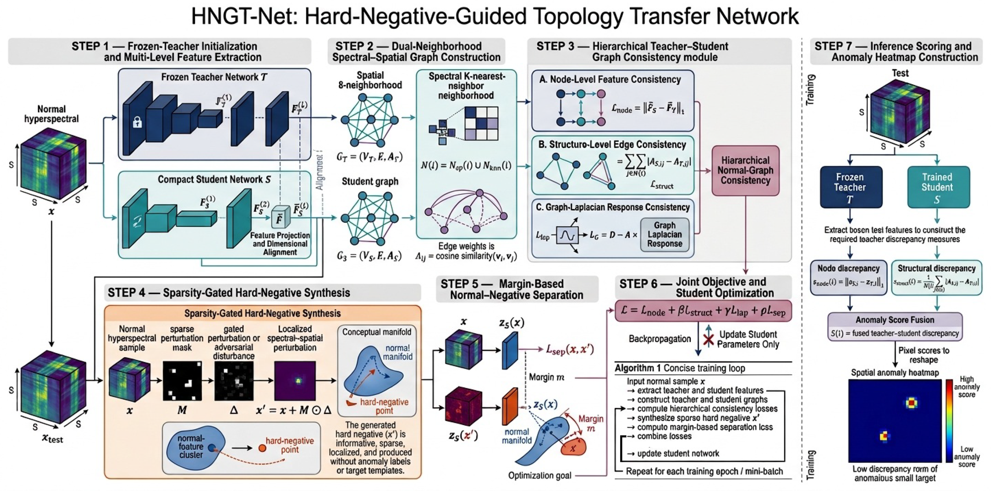
This section reports the experimental validation of the proposed HNGT-Net for hyperspectral small-target detection under the scene-specific normal-only setting. The five evaluation benchmarks and the construction of the purified training data are introduced first.

3.1. Benchmark Datasets and Training Data Preparation

Our evaluation is conducted on four publicly available hyperspectral scenes and one Salinas-derived synthetic benchmark, which are selected to rigorously examine the capability of HNGT-Net in detecting small targets. The collection covers real-world scenes with naturally embedded anomalies as well as a simulated scene with synthetically injected targets, and the scenes differ considerably in composition, spectral characteristics, and background complexity. A property shared by all five benchmarks is that the anomalous targets are sparse and extremely small in footprint, occupying only a tiny portion of the image pixels: their anomaly-to-background pixel ratios range from approximately 0.08% to less than 1%. Such a setting closely reproduces the challenge of revealing unknown small anomalous targets under complex real-world sensing conditions, and therefore provides a demanding test bed for assessing the sensitivity and generalization capability of the proposed method under the scene-specific normal-only setting.

ABU Urban Scene 1 (abu-urban-2). The first dataset originates from the widely adopted Airport–Beach–Urban (ABU) benchmark collection. Its scene was recorded over an urban area in Gainesville by the Airborne Visible/Infrared Imaging Spectrometer (AVIRIS) sensor and comprises $100\times 100$ pixels, with 191 spectral bands retained after the water-absorption and low signal-to-noise ratio bands are removed. Buildings, roads, and vegetation dominate the scene, whereas sparsely distributed vehicles constitute the anomalous targets and cover only a minute fraction of the total pixels.

ABU Urban Scene 2 (abu-urban-4). The second ABU scene was likewise collected by the AVIRIS sensor, but over a different urban area, and it shares the spatial size and band count of abu-urban-2 ($100\times 100$ pixels and 191 spectral bands). Because of its distinct urban layout, heterogeneous background materials, and anomalous objects of varying sizes and spectral signatures, this scene probes the adaptability of the method to different urban configurations under the same small-target constraint.

ABU Coastal Scene (abu-beach-3). The third ABU scene was imaged by the AVIRIS sensor over a coastal area in San Diego and likewise contains $100\times 100$ pixels with 191 spectral bands. Sandy beach, seawater, and coastal vegetation form the background, and the anomalies correspond to small fishing-related objects. Owing to the extremely low anomaly pixel ratio and the high spectral similarity between certain anomalous pixels and the surrounding beach background, this scene is particularly challenging for small-target detection.

Pavia Centre urban benchmark (PaviaC). PaviaC is an urban ROSIS scene collected over central Pavia, Italy. The original scene spans $1096\times 715$ pixels and provides 102 spectral bands covering the wavelength range of 430–860 nm; following the standard protocol in the hyperspectral anomaly detection literature, a representative $100\times 100$ sub-image is cropped from it for evaluation. Buildings, roads, water bodies, and shadow regions are intermixed in the scene, and the anomalous targets—bridge structures and barren earth along the pier—exhibit spectral characteristics distinct from the dominant background materials while accounting for less than 0.5% of the total pixels.

Salinas-derived synthetic benchmark (Salinas simulate). The last benchmark is a synthetic anomaly detection dataset constructed upon the real Salinas scene, which was collected by the AVIRIS sensor over an agricultural test site in Salinas Valley, California. The image consists of $512\times 217$ pixels and 204 spectral bands after the water-absorption and noisy bands are removed. Synthetic anomalous targets are embedded into the genuine background through a linear mixing model: twelve square-shaped anomalous regions are arranged in close proximity to one another, with two targets per side length from 1 to 6 pixels. These regions contain $2\times (1^2+2^2+\cdots +6^2)=182$ anomalous pixels out of $512\times 217=111,104$ total pixels, corresponding to approximately 0.16% of the image. The anomalous signatures produced by this controlled linear spectral mixing remain spectrally coherent with the surrounding background while retaining discriminability for evaluation, making this dataset an extremely challenging micro-target detection scenario. The 1–6 pixel side-length range provides a controlled test bed for assessing the sensitivity of detection methods to targets at and below the spatial-resolution limit.

Table 1. Characteristics of the five hyperspectral benchmarks.

Dataset	Sensor	Size	Bands	GSD (m)	Scene Type	Anomaly Type	Anomaly Ratio
abu-urban-2	AVIRIS	$100\times 100$	191	3.5	Urban	Vehicles	<0.5%
abu-urban-4	AVIRIS	$100\times 100$	191	3.5	Urban	Vehicles	<0.5%
abu-beach-3	AVIRIS	$100\times 100$	191	7.5	Coastal	Fishing objects	<0.5%
PaviaC	ROSIS	$100\times 100$	102	1.3	Urban	Bridge structures	<0.5%
Salinas simulate	AVIRIS	$512\times 217$	204	3.7	Agricultural	Synthetic targets	∼0.16%

summarizes the key characteristics of the five datasets.

Normal-only training data preparation. The adopted supervision protocol requires the training set to contain only purified background pixels. Each benchmark provides a raw hyperspectral cube together with a pixel-level ground-truth (GT) mask, where 1 marks an anomalous pixel and 0 marks background. A background purification procedure is therefore applied to obtain a purely normal training set. In the first step, all background pixels are extracted according to the GT mask ($\mathrm{GT}=0$), and the per-band mean ${\mu }_b$ and standard deviation ${\mathit{\sigma }}_b$ of these pixels are computed. In the second step, the anomalous regions ($\mathrm{GT}=1$) are located and filled with synthetically generated background values, so that anomalous information is eliminated while local spatial continuity is preserved. Concretely, an anomalous pixel at spectral band b is replaced by ${\mu }_b+{ϵ}_b$, where ${ϵ}_b\sim \mathcal{N}(0,{\eta }^2{\sigma }_b^2)$, and $\eta =0.2$ is a noise scaling factor. The injected Gaussian perturbations preserve stochastic spectral variability in the filled pixels, avoiding unrealistically smooth replacements and reducing the risk that the network memorizes artificial holes. The purified image is then stored as a .mat file under the variable name data, and its GT mask is reset to all zeros to mark a completely anomaly-free image. Consequently, the student network is exposed exclusively to normal spectral–spatial patterns during training, which enforces the normal-only supervision constraint. The GT mask is used only to construct the purified training image and is not used in the optimization objective. Because purification and model training are performed separately for each evaluation scene, whereas testing uses the corresponding original image, this protocol is more accurately characterized as scene-specific normal-only, or transductive, learning. It should not be interpreted as strict cross-scene, cross-sensor, or cross-domain transfer. A strict transfer protocol would require training on one set of scenes or sensors and testing on completely different scenes or sensors without target-scene purification or adaptation; evaluating such a protocol constitutes an important direction for future work.

Normal-only training data preparation. The adopted supervision protocol requires the training data to contain only normal background information. For each benchmark, the original hyperspectral cube is denoted by $\mathit{X}\in {\mathbb{R}}^{H\times W\times B}$, where H, W, and B represent the image height, width, and number of spectral bands, respectively. The corresponding pixel-level ground-truth (GT) mask uses 1 to mark an anomalous pixel and 0 to mark a background pixel. To prevent anomalous spectra from participating in the training process, a background-purification procedure is performed before the input cube is supplied to HNGT-Net.

First, all pixels satisfying $\mathrm{GT}=0$ are extracted from the original cube. Let ${\Omega }_{\mathrm{bg}}=\{i\mid \mathrm{GT}\left(i\right)=0\}$ and ${\Omega }_{\mathrm{an}}=\{i\mid \mathrm{GT}\left(i\right)=1\}$ denote the sets of background and anomalous pixels, respectively. For the bth spectral band, the mean and standard deviation of the background pixels are calculated as

$${\mathit{\mu }}_b={\displaystyle \frac{1}{|{\Omega }_{\mathrm{bg}}|}}\sum _{i\in {\Omega }_{\mathrm{bg}}}{\mathit{X}}_{i,b},{\mathit{\sigma }}_b=\sqrt{{\displaystyle \frac{1}{|{\Omega }_{\mathrm{bg}}|}}{\sum }_{i\in {\Omega }_{\mathrm{bg}}}{\left({\mathit{X}}_{i,b}-{\mathit{\mu }}_b\right)}^2}.$$

(22)

These statistics characterize the band-wise spectral distribution of the normal background in the current scene.

Second, all positions satisfying $\mathrm{GT}=1$ are located, and their original anomalous spectra are removed. Direct deletion is not adopted because it would alter the spatial dimensions of the hyperspectral cube. Likewise, replacing every anomalous pixel with the same mean spectrum would produce unnaturally smooth regions that could be memorized by the network. Instead, each anomalous pixel is filled with a stochastic background value. Specifically, the purified value at anomalous pixel i and spectral band b is generated as

$${\tilde{\mathit{X}}}_{i,b}={\mathit{\mu }}_b+{\mathit{ϵ}}_{i,b},{\mathit{ϵ}}_{i,b}\sim \mathcal{N}\left(0,{\eta }^2{\mathit{\sigma }}_b^2\right),i\in {\Omega }_{\mathrm{an}},$$

(23)

where $\eta =0.2$ is the noise-scaling factor used in all experiments. The original values of the background pixels are retained:

$${\tilde{\mathit{X}}}_{i,b}={\mathit{X}}_{i,b},i\in {\Omega }_{\mathrm{bg}}.$$

(24)

The band-dependent Gaussian perturbation preserves a limited amount of stochastic spectral variability in the filled pixels. Consequently, the replacement regions remain statistically compatible with the surrounding background and do not form constant artificial holes. If a scene contains no labeled anomalous pixel, the original hyperspectral cube is directly retained.

After the replacement operation, the purified cube $\tilde{\mathit{X}}$ preserves the same spatial and spectral dimensions as the original image. The associated GT mask is reset to an all-zero matrix, indicating that every spatial position in the resulting training cube is treated as normal. Therefore, the original GT information is used only during this offline purification procedure and is not provided to the network during parameter optimization.

Before training, invalid numerical entries, including NaN and infinite values, are replaced with finite values. Each spectral band of the purified cube is then independently normalized to the interval $[0,1]$:

$${\widehat{\mathit{X}}}_{i,b}={\displaystyle \frac{{\tilde{\mathit{X}}}_{i,b}-{min}_j{\tilde{\mathit{X}}}_{j,b}}{{max}_j{\tilde{\mathit{X}}}_{j,b}-{min}_j{\tilde{\mathit{X}}}_{j,b}+\epsilon }},$$

(25)

where $\epsilon$ is a small constant used to avoid numerical instability. If a spectral band has zero dynamic range, its denominator is set to one. The normalized cube is subsequently rearranged from $H\times W\times B$ to $B\times H\times W$ to match the network input format.

Because each benchmark contains one complete hyperspectral scene, the entire purified cube is treated as one training sample, with the batch size set to 1 and sample shuffling disabled. The number of input channels is automatically adjusted according to the number of spectral bands in the current scene. During each training epoch, the normalized normal cube is forwarded through the fixed teacher branch and the trainable student branch. The teacher provides the reference spectral–spatial representations, whereas the student and its feature-projection layer are optimized using the joint objective described in Section 2. Only the student-related parameters receive gradient updates. Adam is adopted for optimization, and the gradient norm is clipped to 0.5 before each parameter update to improve numerical stability. An iteration is discarded if the computed loss is NaN, infinite, or greater than ${10}^6$. After the prescribed number of epochs, the scene-specific model parameters are saved for subsequent anomaly detection. Consequently, the complete preparation and training sequence is given by raw-cube loading, background-statistics estimation, anomalous-pixel replacement, band-wise normalization, teacher–student forward propagation, loss calculation, and student-parameter updating.

3.2. Detection Performance Comparison

The experimental platform is the Wuhan node of the National Supercomputing Internet (SCNet), administered by Sugon Intelligence Computing Information Technology Co., Ltd., Beijing, China. Every run is executed inside a Kubernetes-orchestrated container instance allocated with seven cores of a Hygon C86-7380 processor (32-core, 2.0 GHz base frequency), 60 GB of DDR4 system memory, and one Hygon Deep Computing Unit (DCU) accelerator built on the AMD CDNA-compatible gfx906 architecture with 16 GB of HBM2 memory. GPU acceleration is delivered through the ROCm-compatible Hygon DeepTensorKit (DTK) software stack, version 24.04, and the environment variable HSA_OVERRIDE_GFX_VERSION=9.0.6 is exported so that the ROCm runtime correctly recognizes the gfx906 device. All compared models are implemented in Python 3 and executed on a single DCU card within this containerized environment.

Benchmarking is performed against six representative detectors, covering two classical shallow models and four recent deep learning-based models. The former category comprises the Local Reed–Xiaoli detector (LRX) [12] and the Collaborative Representation-based Detection (CRD) [21], while the latter comprises the autoencoder-driven anomaly detection network (Auto-AD) [44], the Deep Feature Aggregation Network for Hyperspectral Anomaly Detection (DFAN-HAD) [45], the non-local and local feature-coupled self-supervised network (NL2Net) [46], and the Dual-window-inspired reconstruction Network (DirectNet) [47].

AUC-based quantitative evaluation.

Table 2. AUC results of HNGT-Net and six competing detectors on five hyperspectral benchmarks. Bold entries denote the best score for each dataset and the best overall average.

Dataset	Traditional Algorithms		Deep Learning Algorithms				HNGT-Net
	LRX	CRD	Auto-AD	DFAN-HAD	NL2Net	DirectNet
abu-urban-2	0.9038	0.9762	0.7479	0.9734	0.9994	0.9897	0.9989
abu-urban-4	0.9059	0.9111	0.5444	0.9625	0.9966	0.9630	0.9856
abu-beach-3	0.9991	0.9985	0.9276	0.9999	0.9259	0.9924	0.9935
PaviaC	0.9271	0.9957	0.8924	0.9988	0.9997	0.9954	0.9991
Salinas simulate	0.9821	0.9821	0.9261	0.9857	0.9279	0.9945	0.9996
Mean	0.9436	0.9727	0.8077	0.9841	0.9699	0.9870	0.9953

reports the detection accuracy of HNGT-Net and all baseline detectors across the five benchmarks. With an average AUC of 0.9953, HNGT-Net ranks first among all compared methods, exceeding the strongest baseline DirectNet (0.9870) by 0.83 percentage points and outperforming the classical LRX (0.9436) and CRD (0.9727). Equally importantly, the per-dataset AUCs of HNGT-Net lie within 0.9856–0.9996; their population standard deviation is approximately 0.00535, the smallest among the compared methods. Such stability suggests that the three-level consistency-transfer strategy learns transferable normal-feature representations that remain reliable under diverse sensing scenarios.

The remaining methods behave considerably less evenly. Driven purely by reconstruction error, Auto-AD records the lowest mean AUC (0.8077) and collapses on the abu-urban-4 scene (0.5444), which exposes the inherent fragility of reconstruction-only discrimination when small targets are embedded in heterogeneous backgrounds. NL2Net posts the best individual scores on abu-urban-2 (0.9994), abu-urban-4 (0.9966), and PaviaC (0.9997), yet it degrades markedly on abu-beach-3 (0.9259) and Salinas simulate (0.9279), revealing a pronounced sensitivity to scene-dependent spectral characteristics. DFAN-HAD follows a similar pattern: it leads on abu-beach-3 (0.9999) but falls to 0.9625 on abu-urban-4. Taken together, these results indicate that HNGT-Net achieves a favorable balance between detection accuracy and stability across the evaluated scenes under scene-specific normal-only conditions.

Because overall AUC accumulates detection performance across the entire false-alarm range, it tends to saturate when ROC curves lie close to the upper-left corner and therefore provides limited information about performance in the low-FPR regime that is critical for real-world surveillance. To obtain a more operationally meaningful assessment, we additionally report the detection probability $P_d$ evaluated at fixed false-alarm rates $P_{fa}\in \{{10}^{-4},{10}^{-3},{10}^{-2}\}$. The results are summarized in

Table 3. Detection performance under low false-alarm-rate constraints. AUC denotes the area under the full ROC curve; $P_d$ denotes the detection probability at fixed false-alarm rates ($P_{fa}$).

Dataset	AUC	${\mathit{P}}_{\mathit{d}}$@${\mathit{P}}_{\mathit{fa}}={10}^{-4}$	${\mathit{P}}_{\mathit{d}}$@${\mathit{P}}_{\mathit{fa}}={10}^{-3}$	${\mathit{P}}_{\mathit{d}}$@${\mathit{P}}_{\mathit{fa}}={10}^{-2}$
abu-urban-2	0.9989	0.2516	0.5613	1.0000
abu-urban-4	0.9856	0.0882	0.1985	0.4779
abu-beach-3	0.9935	0.1818	0.3636	0.7273
PaviaC	0.9991	0.1395	0.6279	1.0000
Salinas simulate	0.9996	0.6216	0.9027	1.0000

.

As shown in the table, although AUC spans a narrow interval of 0.9856–0.9996, the $P_d$ metrics uncover substantial scene-dependent differentiation that is invisible to the full AUC. At the most stringent threshold $P_{fa}={10}^{-4}$, the proposed method attains $P_d=0.6216$ on Salinas simulate, demonstrating that the topology-transfer objective and hard-negative separation preserve sufficient discriminative cues for 1–6-pixel micro-targets even under a one-in-ten-thousand false-alarm constraint. PaviaC also exhibits strong low-$P_{fa}$ performance ($P_d=0.1395$ at $P_{fa}={10}^{-4}$, rising sharply to $0.6279$ at $P_{fa}={10}^{-3}$), confirming that the structural and Laplacian consistency terms effectively capture the bridge-structure anomalies in this spectrally heterogeneous scene.

On abu-urban-2 and abu-beach-3, the method achieves moderate $P_d$ values at $P_{fa}={10}^{-4}$ (0.2516 and 0.1818, respectively) and improves monotonically with relaxed $P_{fa}$, reaching $0.7273$ on abu-beach-3 at $P_{fa}={10}^{-2}$. The abu-urban-4 scene presents the greatest challenge: its anomalous targets are extremely sparse and spectrally subtle against a complex urban background, which intrinsically suppresses $P_d$ at ultra-low $P_{fa}$. Nevertheless, the method recovers to $P_d=0.4779$ at $P_{fa}={10}^{-2}$ while maintaining AUC $=0.9856$, indicating that the learned topology still encodes useful discriminative information once a modest false-alarm tolerance is permitted.

Moreover, three of the five scenes (abu-urban-2, PaviaC, and Salinas simulate) achieve perfect detection ($P_d=1.0000$) at $P_{fa}={10}^{-2}$, which confirms that the proposed framework can eliminate missed detections entirely when the operational system tolerates a one-percent false-alarm rate. Collectively, these low-$P_{fa}$ results demonstrate that HNGT-Net maintains practical detection capability for micro-scale targets under the stringent false-alarm constraints required by real-world remote-sensing surveillance, well beyond what saturated AUC values alone can convey.

To evaluate the sensitivity of HNGT-Net to micro-scale targets of varying spatial extent, the Salinas-derived synthetic dataset is further analyzed by grouping anomalous targets according to their side lengths. The scene contains twelve synthetic anomalous regions that can be stratified into six size classes from $1\times 1$ to $6\times 6$ pixels, with two targets per class.

Table 4. Detection performance on the Salinas-derived synthetic dataset stratified by target size. Each group contains two anomalous targets whose side lengths range from 1 to 6 pixels.

Target Size (px)	Count	Total Pixels	AUC	${\mathit{P}}_{\mathit{d}}$@${\mathit{P}}_{\mathit{fa}}={10}^{-4}$	${\mathit{P}}_{\mathit{d}}$@${\mathit{P}}_{\mathit{fa}}={10}^{-3}$	${\mathit{P}}_{\mathit{d}}$@${\mathit{P}}_{\mathit{fa}}={10}^{-2}$
$1\times 1$	2	3	0.9982	0.0000	0.3333	1.0000
$2\times 2$	2	8	0.9993	0.5000	0.6250	1.0000
$3\times 3$	2	18	0.9989	0.6667	0.8889	0.9444
$4\times 4$	2	33	0.9995	0.7273	0.9091	0.9697
$5\times 5$	2	50	0.9996	0.6600	0.8600	1.0000
$6\times 6$	2	73	0.9998	0.7945	0.9589	1.0000
All	12	185	0.9996	0.7081	0.8919	0.9892

reports the detection performance for each size group.

Several clear trends emerge from the stratified results. First, detection capability improves monotonically with target size at stringent false-alarm rates. At $P_{fa}={10}^{-4}$, the $1\times 1$ pixel targets are not detected ($P_d=0.0000$), reflecting the fundamental difficulty of resolving single-pixel anomalies against complex agricultural backgrounds. As target size increases to $2\times 2$ pixels, $P_d$ rises sharply to $0.5000$, and for $6\times 6$ pixels it reaches $0.7945$. This progressive improvement confirms that the topology-transfer objective successfully aggregates spectral–spatial evidence from neighboring pixels, enabling reliable detection once the target occupies a sufficient spatial footprint.

Second, at the relaxed threshold $P_{fa}={10}^{-2}$, even the smallest $1\times 1$ targets achieve perfect detection ($P_d=1.0000$), and only the $3\times 3$ group falls slightly below saturation ($P_d=0.9444$). This indicates that while sub-pixel and single-pixel targets remain challenging under ultra-low false-alarm constraints, the method can recover them entirely once a modest false-alarm tolerance is permitted. The AUC values across all size groups remain consistently high ($0.9982$–$0.9998$), demonstrating that the ranking-based metric is less sensitive to target size than the operationally relevant $P_d$ metrics.

Third, the $4\times 4$ and $6\times 6$ groups exhibit the strongest low-$P_{fa}$ performance ($P_d=0.7273$ and $0.7945$ at $P_{fa}={10}^{-4}$, respectively), suggesting that targets occupying sixteen or more pixels provide sufficient spectral–spatial contrast for the graph-Laplacian and structural consistency terms to discriminate effectively. Conversely, the intermediate $5\times 5$ group shows slightly lower $P_d$ at $P_{fa}={10}^{-4}$ ($0.6600$) than the $4\times 4$ group, which may be attributed to the particular spectral mixture coefficients and background configuration at those target locations.

Overall, these stratified results validate that HNGT-Net maintains robust detection capability for micro-scale targets down to $2\times 2$ pixels under stringent false-alarm constraints, and achieves perfect or near-perfect detection for all target sizes at $P_{fa}={10}^{-2}$. The degradation for single-pixel targets at ultra-low $P_{fa}$ is expected and consistent with the fundamental limits of spatial resolution in hyperspectral anomaly detection.

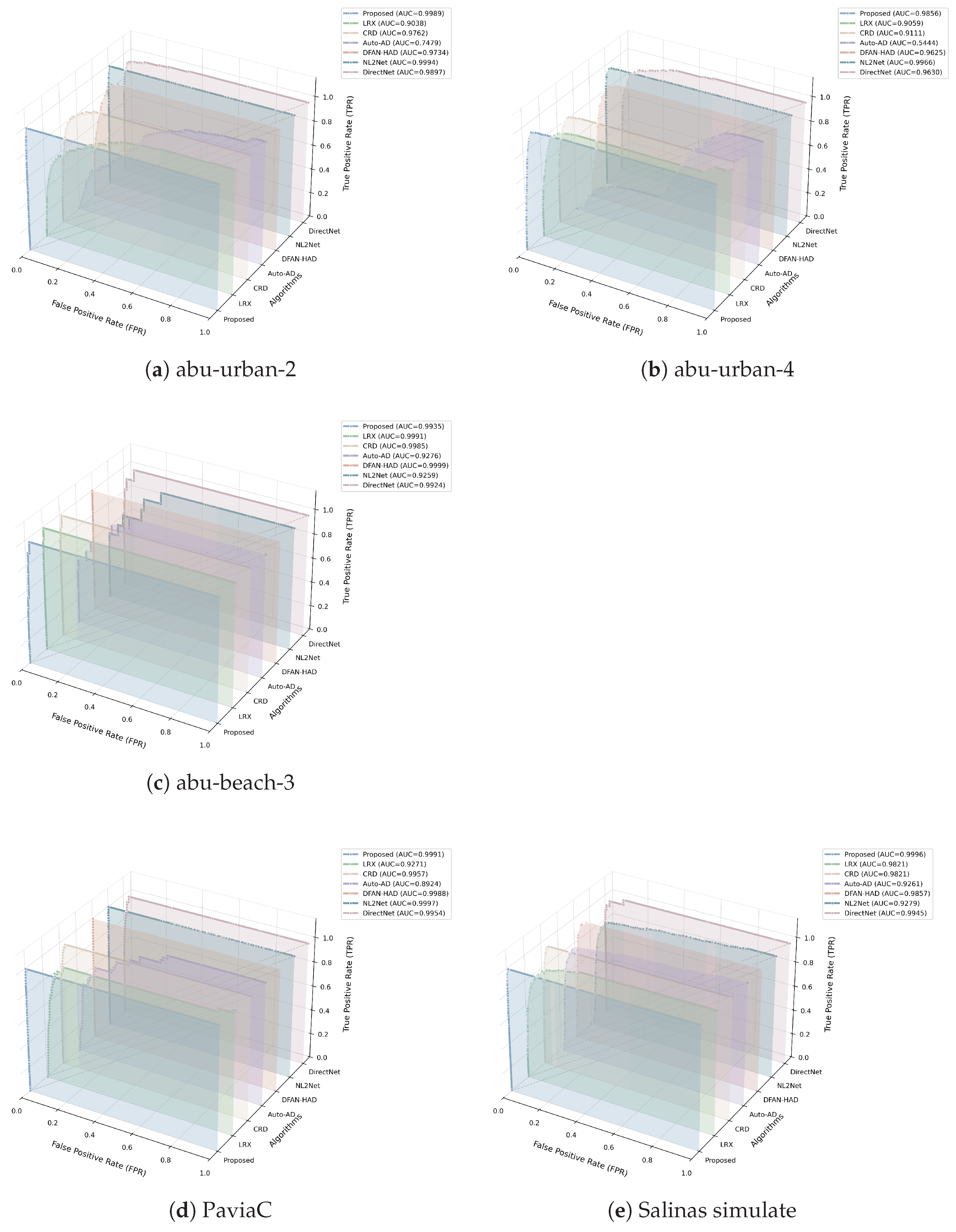
ROC behavior. Figure 2 presents the three-dimensional waterfall ROC curves of HNGT-Net and the competing methods on the five benchmark scenes. Overall, HNGT-Net remains within the leading group across all datasets, demonstrating a favorable trade-off between the true-positive rate and the false-positive rate. On abu-urban-2, HNGT-Net achieves an AUC of 0.9989 and performs comparably to the best-performing NL2Net (0.9994), while outperforming the remaining detectors. On abu-urban-4, HNGT-Net obtains an AUC of 0.9856, ranking second behind NL2Net (0.9966) and maintaining a clear advantage over the other competing methods. On PaviaC, the ROC curves of HNGT-Net, NL2Net, and DFAN-HAD are concentrated near the upper-left region, with AUC values of 0.9991, 0.9997, and 0.9988, respectively, indicating similarly strong detection performance at low false-positive rates. For abu-beach-3, DFAN-HAD, LRX, and CRD achieve the three highest AUC values, whereas HNGT-Net remains competitive with an AUC of 0.9935 and slightly exceeds DirectNet (0.9924). On Salinas simulate, HNGT-Net provides the best overall performance, achieving an AUC of 0.9996 and a rapidly rising ROC curve, followed by DirectNet with an AUC of 0.9945. These results show that HNGT-Net provides consistently high detection accuracy across scenes, although the relative advantages of individual competing methods vary with the spectral and spatial characteristics of each dataset.

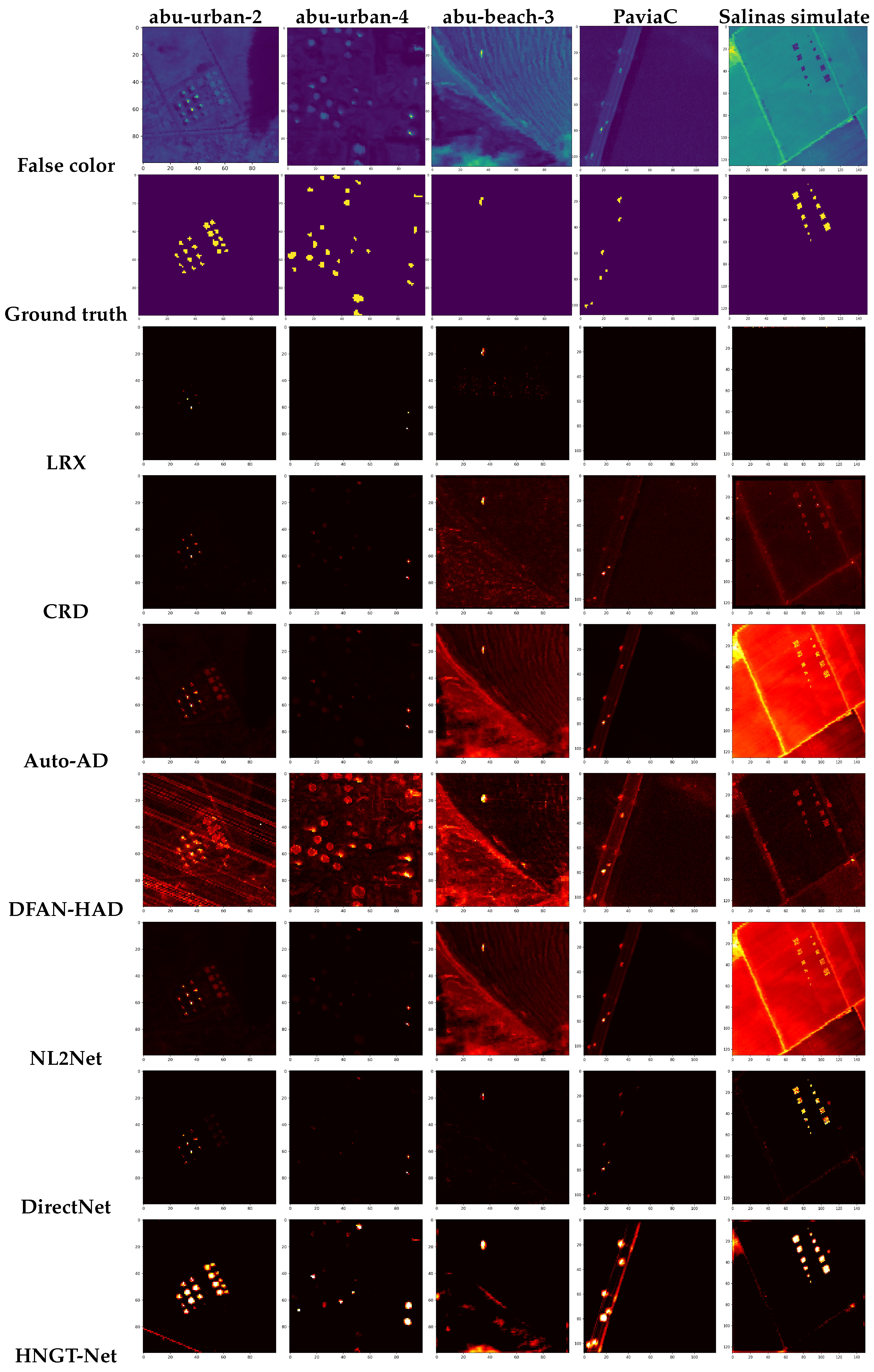
Visual inspection of detection maps. Figure 3 provides a scene-by-scene visual comparison of the anomaly score maps produced by all methods, revealing several consistent patterns.

On the abu-urban-2 scene, HNGT-Net renders the anomalous vehicle targets as compact, high-intensity bright spots embedded in an almost entirely dark background. LRX and CRD, by contrast, respond with only a few dim, barely perceptible pixels that convey little of the true spatial extent of the anomalies. Auto-AD produces diffuse background activation together with blurred anomaly contours; DFAN-HAD overlays the map with stripe-shaped background artifacts that heavily mask the targets; and NL2Net, although it detects most anomalies, leaves a visible background haze that reduces spatial fidelity.

The abu-urban-4 scene separates the methods even more clearly. LRX, CRD, NL2Net, and DirectNet yield only faint, poorly defined responses and therefore fail to localize the anomalous targets in any meaningful way. DFAN-HAD finds the targets but at relatively low contrast, and Auto-AD raises heavy background clutter that conceals them. HNGT-Net instead delivers the brightest and most compact anomaly localization while keeping background interference minimal.

On the abu-beach-3 coastal scene, every method succeeds in detecting the anomalous fishing-related targets, albeit with markedly different background quality. LRX and NL2Net offer clean backgrounds with well-delimited target regions. HNGT-Net again returns the brightest and most compact anomaly response, at the cost of a small amount of background misactivation along the shoreline. CRD, Auto-AD, and DFAN-HAD, on the other hand, are hampered by severe clutter induced by sand textures, which partially buries the true anomalies.

For the PaviaC scene, LRX produces no usable anomaly response at all. CRD, Auto-AD, DFAN-HAD, and NL2Net suppress the background insufficiently, so that background structures mingle with target localization in cluttered detection maps. DirectNet keeps the background clean and correctly detects all bridge-structure targets along the diagonal pier, although its anomaly regions are less crisp than those of HNGT-Net. The proposed HNGT-Net provides the brightest and most compact target localization; its only visible flaw is that one edge of the bridge structure is mistakenly highlighted as anomalous.

On the Salinas simulate scene, LRX reveals almost none of the six synthetically embedded anomalous squares. CRD, Auto-AD, DFAN-HAD, and NL2Net respond excessively along the agricultural field boundaries, which seriously undermines the visibility of the true targets. Both DirectNet and HNGT-Net suppress the background cleanly and recover all anomalous targets, with HNGT-Net yielding markedly brighter and more sharply delineated anomaly regions than DirectNet. Overall, these qualitative comparisons confirm that the topology-transfer learning and hard-negative separation mechanisms jointly equip HNGT-Net with accurate detection and high spatial fidelity for small targets across diverse sensing scenarios.

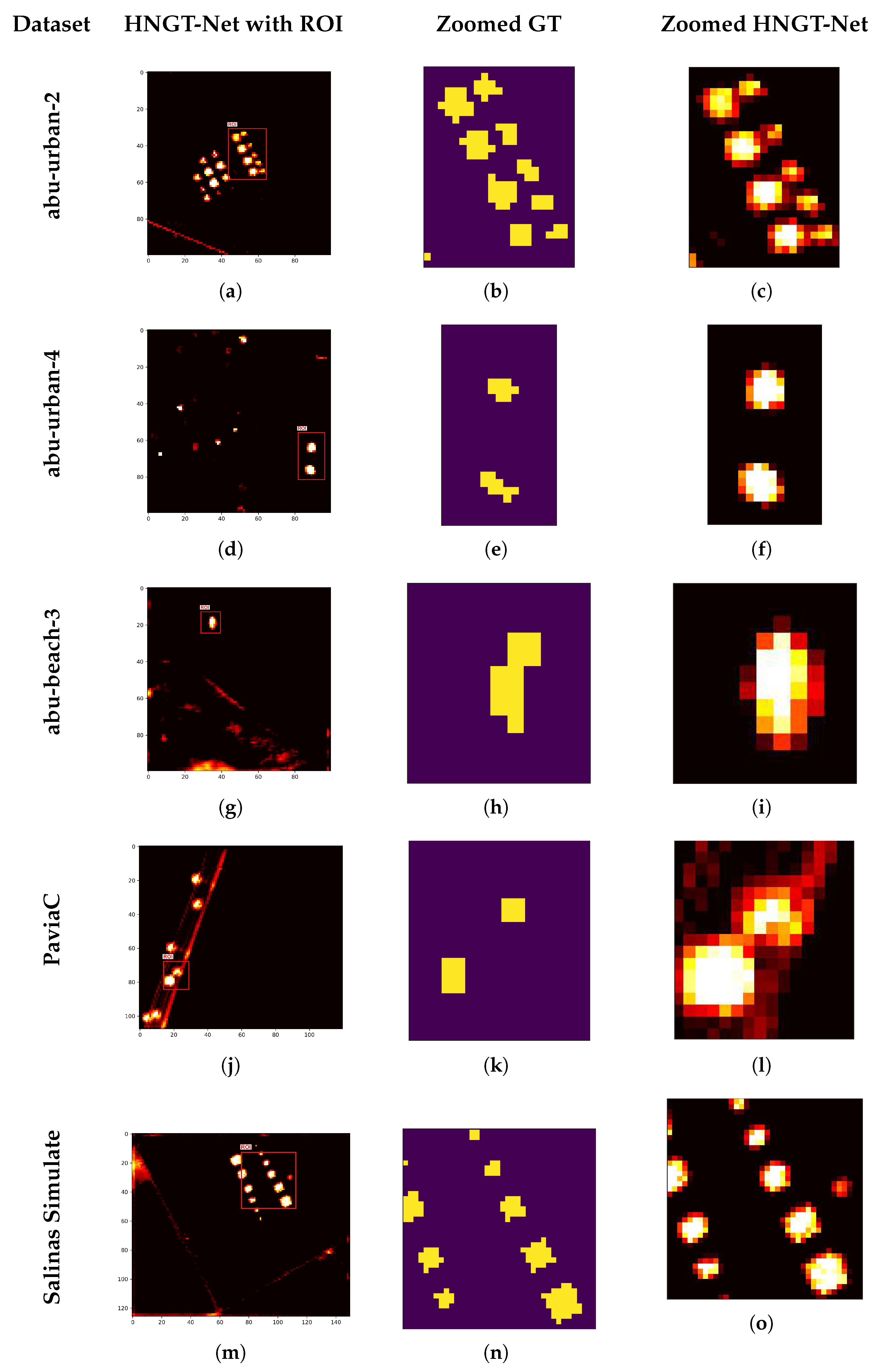
Detailed visual analysis of the selected regions of interest. To provide a more intuitive assessment of spatial detection quality, Figure 4 presents enlarged comparisons between the GT maps and the HNGT-Net detection results. Each row corresponds to one dataset, while the three columns show the complete detection map with the selected region of interest (ROI), the enlarged GT map, and the corresponding enlarged HNGT-Net response, respectively. These enlarged regions permit target localization, boundary preservation, response continuity, and background interference to be examined at the pixel level. For the ABU-Urban-2 scene (Figure 4a–c), the selected ROI contains a dense group of spatially adjacent anomalies with different shapes and sizes. HNGT-Net assigns strong responses to most anomalous objects and preserves their overall spatial distribution. Several closely spaced targets remain distinguishable instead of being merged into one continuous response. Some detected regions extend slightly beyond their GT boundaries, indicating limited response diffusion around high-contrast targets; nevertheless, the dominant responses remain concentrated within the actual anomalous region, while the surrounding homogeneous background is largely suppressed. For ABU-Urban-4 (Figure 4d–f), the enlarged region includes isolated anomalies with noticeably different spatial extents. HNGT-Net produces prominent responses at the corresponding locations and maintains the separation between these objects. Both compact targets and relatively large anomalies can be distinguished from the surrounding background, showing that the detector is not restricted to a single target scale. Although weak residual responses occur around several target boundaries, the response maxima remain spatially consistent with the GT locations. In ABU-Beach-3 (Figure 4g–i), the GT contains one dominant compact anomaly in the selected ROI. HNGT-Net clearly highlights this object and reproduces its vertically elongated spatial structure. The highest anomaly scores occur in the target interior, whereas the responses gradually decrease near its boundary, demonstrating accurate localization against the relatively uniform beach background. Weak responses remain outside the ROI, particularly near scene boundaries and locally heterogeneous structures, but their intensities are substantially lower than that of the true target. For PaviaC (Figure 4j–l), the selected ROI contains several small anomalies close to elongated urban structures. HNGT-Net assigns high scores to the principal anomalous objects and retains their relative positions and approximate spatial extents. The enlarged result also reveals responses along some neighboring linear structures. Such responses arise from the strong spectral–spatial contrast of urban edges and narrow human-made materials, which may locally resemble anomalies. Despite this structured-background interference, the true anomalies generally exhibit brighter and more compact responses and therefore remain visually distinguishable. For the Salinas simulated scene (Figure 4m–o), the ROI contains multiple simulated anomalies with different sizes and irregular shapes. HNGT-Net detects most targets with strong and spatially compact responses, including both small isolated objects and larger anomaly clusters. The response centers agree well with the GT locations, and adjacent targets remain separable. Meanwhile, the complete map exhibits residual activations along image boundaries and diagonal background structures, indicating that high-contrast field boundaries remain challenging without obscuring the principal anomaly cluster. Overall, the enlarged comparisons demonstrate consistent spatial correspondence between HNGT-Net responses and the GT maps across isolated targets, dense target clusters, and anomalies of different scales. The method generally produces compact high-score regions at true anomaly locations while suppressing most homogeneous background pixels. The remaining discrepancies mainly appear as slight boundary expansion around strong targets or weak responses to high-contrast edges and linear structures. These observations provide a detailed and balanced account of both the localization capability of HNGT-Net and the background conditions under which residual false responses may occur.

3.3. Computational Complexity and Runtime Analysis

The computational efficiency and deployment feasibility of the proposed HNGT-Net are examined from four complementary angles: theoretical time complexity, per-module FLOPs decomposition, parameter and computation compression between the teacher and student networks, and space complexity.

Theoretical Time Complexity. Consider an input hyperspectral image of size $H\times W\times B$, with $N=HW$ denoting the total number of pixels. The asymptotic inference complexity of HNGT-Net is contrasted with that of representative competitors as follows:

• LRX and CRD demand $O(B·N·w^2)$ operations per pixel, where w denotes the sliding-window size. The quadratic growth with respect to w makes these methods prohibitively expensive on large scenes.
• Pure deep networks (Auto-AD, DFAN-HAD) incur $O(B·N·C^2)$ FLOPs, where C denotes the feature-channel width. Although the window-squared term disappears, the cost remains heavy once C becomes large.
• HNGT-Net decomposes into four additive terms:

  $${\mathcal{C}}_{\text{HNGT-Net}}=\underset{\mathrm{Teacher}\mathrm{forward}}{\underbrace{O(B·N·C_t)}}+\underset{\mathrm{Student}\mathrm{forward}}{\underbrace{O(B·N·C_s)}}+\underset{\mathrm{KNN}\mathrm{graph}\mathrm{build}}{\underbrace{O(N·KlogN)}}+\underset{\mathrm{Laplacian}\mathrm{response}}{\underbrace{O(N·K)}},$$

  (26)

  where $C_t$ and $C_s$ denote the teacher and student channel widths, respectively, and K is the number of nearest neighbors. All four terms grow linearly with the pixel count N; therefore, the overall pipeline avoids the window-squared penalty of statistical methods, although the frozen teacher remains part of the inference stack and contributes the largest share of the measured FLOPs.

Per-Module FLOPs Decomposition. The estimated inference FLOPs of each HNGT-Net module on a $100\times 100\times 191$ input (the standard crop size adopted throughout our experiments) are listed in

Table 5. Module-wise inference FLOPs of HNGT-Net for a $100\times 100\times 191$ input, computed with $3\times 3$ convolutional kernels and $K=20$ nearest neighbors.

Module	Complexity	Est. FLOPs	Proportion
Teacher encoder (T)	$O\left(BN{C}_t\right)$	∼1.33 G	68.4%
Student encoder (S)	$O\left(BN{C}_s\right)$	∼0.61 G	31.4%
Projection head (g)	$O\left(N{C}_s{C}_t\right)$	∼1.3 M	<0.1%
KNN graph build	$O(NKlogN)$	∼2.8 M	0.1%
Laplacian response	$O\left(NK\right)$	∼0.2 M	<0.1%
Divergence compute	$O\left(N{C}_t\right)$	∼0.2 M	<0.1%
Total	$O\left(N(B(C_t+C_s)+C_s{C}_t+KlogN+K+C_t)\right)$	∼1.95 G	100%

. The convolutional encoders absorb the overwhelming majority of the computational budget, whereas the graph-structured operations jointly contribute less than $1\%$ of the total.

Parameter and Computation Compression. The teacher network $T(·)$ is built as a three-layer encoder with channel configurations $[B,64,32,16]$, amounting to roughly 0.21 Mparameters, whereas the student network $S(·)$ halves every layer to $[B,32,16,8]$ and appends a lightweight projection head $g(·)$, totaling only about 0.02 M parameters. The resulting parameter compression ratio reaches 10.5×.

At the layer level, width halving predicts an approximately fourfold reduction in convolutional FLOPs. In the implemented three-layer encoders, the measured FLOPs decrease from 1.33 G for the teacher to 0.61 G for the student, corresponding to a 2.18× encoder-level reduction; the difference from the ideal factor of four arises from input/output channel terms and auxiliary operations. Because the teacher remains active during inference, the 10.5× figure should be interpreted as student-side parameter compression, while the complete teacher–student stack retains a compact footprint of approximately 0.23 M parameters. The sparse graph operations add less than $1\%$ of the total FLOPs.

Space Complexity. The peak memory footprint at inference time scales as

$$\mathcal{M}=O\left(N·(B+C_t+C_s+K)\right),$$

(27)

with the four terms corresponding respectively to the input image ($N·B$), the teacher feature map ($N·C_t$), the student feature map ($N·C_s$), and the sparse adjacency storage ($N·K$ non-zero entries in CSR format). Storing the adjacency matrix sparsely, rather than as a dense $N\times N$ matrix, eliminates the $O\left(N^2\right)$ memory blow-up that would otherwise preclude deployment on high-resolution scenes.

Scalability Analysis. Owing to its linear-in-N complexity, HNGT-Net scales gracefully to larger image sizes. On the $100\times 100$ crops evaluated in this paper, KNN graph construction accounts for less than $0.2\%$ of the total FLOPs. When N grows to ${10}^6$ pixels (e.g., $1000\times 1000$ full-scene inference), the convolutional terms increase linearly ($\times 100$), while the KNN term grows as $NlogN$ ($\times 100\times log100\approx \times 460$) and gradually becomes a non-negligible fraction. In such regimes, approximate KNN algorithms (e.g., locality-sensitive hashing or FAISS-based fast search) can replace exact KNN without materially affecting detection accuracy. Conversely, enlarging the spectral dimension B affects only the first convolutional layer and leaves the graph structure intact, which makes HNGT-Net particularly attractive for high-spectral-resolution sensors.

Measured runtime. All methods were timed on the same SCNet container and hardware configuration described above, with one DCU card used per run. For reproducibility, all dual-window sizes are reported as inner window × outer window. LRX uses $7\times 11$ for abu-urban-2, $7\times 13$ for abu-urban-4, $23\times 27$ for abu-beach-3, $23\times 27$ for PaviaC, and $5\times 27$ for Salinas simulate. CRD uses $7\times 11$ for abu-urban-2, $7\times 13$ for abu-urban-4, $9\times 13$ for abu-beach-3, $3\times 5$ for PaviaC, and $3\times 15$ for Salinas simulate. The inference runtimes (in seconds) of all competing algorithms on the five benchmark datasets are reported in

Table 6. Measured inference time (s) on five hyperspectral benchmarks. Bold and underlined entries indicate the fastest and second-fastest methods, respectively.

Dataset	LRX	CRD	Auto-AD	DFAN-HAD	NL2Net	DirectNet	Ours
abu-urban-2	1568.80	1041.13	13.76	20.34	1.59	0.13	2.31
abu-urban-4	1610.73	1572.66	13.59	19.44	0.05	0.13	2.27
abu-beach-3	38.05	1989.67	16.29	20.98	1.63	0.12	2.28
PaviaC	1730.12	2604.32	13.52	4.81	0.10	0.11	2.24
Salinas simulate	340.43	108.16	20.86	9.46	0.10	0.12	2.35
Mean	1057.63	1463.19	15.60	15.01	0.69	0.12	2.29

. HNGT-Net averages 2.29 s per scene, which is roughly 462× faster than LRX and 639× faster than CRD, since the shallow statistical methods depend on computationally expensive sliding-window operations. Within the deep learning group, DirectNet records the shortest average runtime (0.12 s), followed by NL2Net (0.69 s); HNGT-Net ranks third, being approximately 3.3× slower than NL2Net and 18.8× slower than DirectNet. This additional overhead stems from the graph construction and Laplacian computation introduced by the topology-transfer learning pipeline. Even so, the runtime of HNGT-Net remains well within the acceptable range for practical deployment, and the modest extra cost is amply compensated by the detection accuracy gains reflected in the leading mean AUC of 0.9953.

3.4. Hyperparameter Sensitivity and Selection

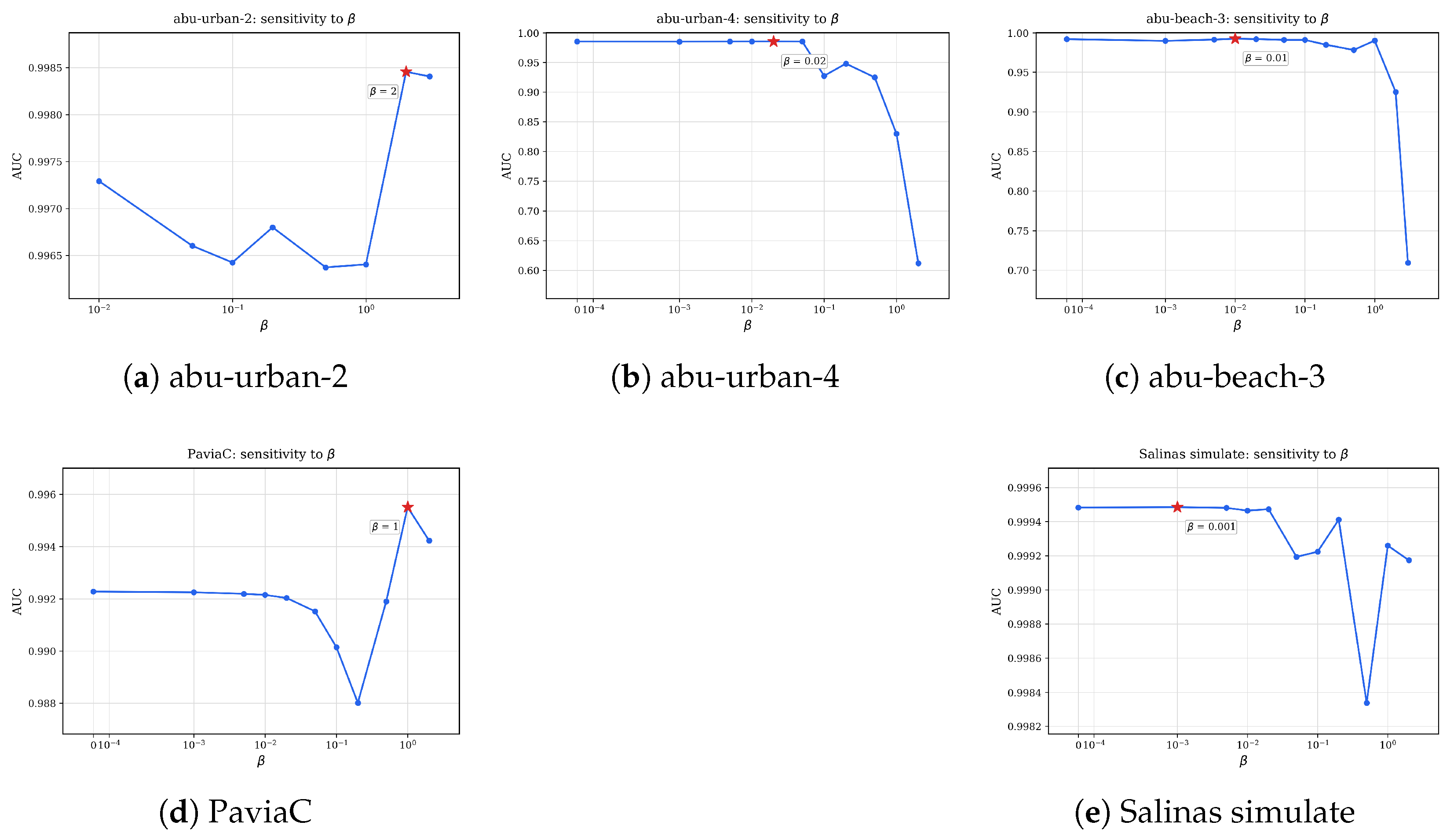
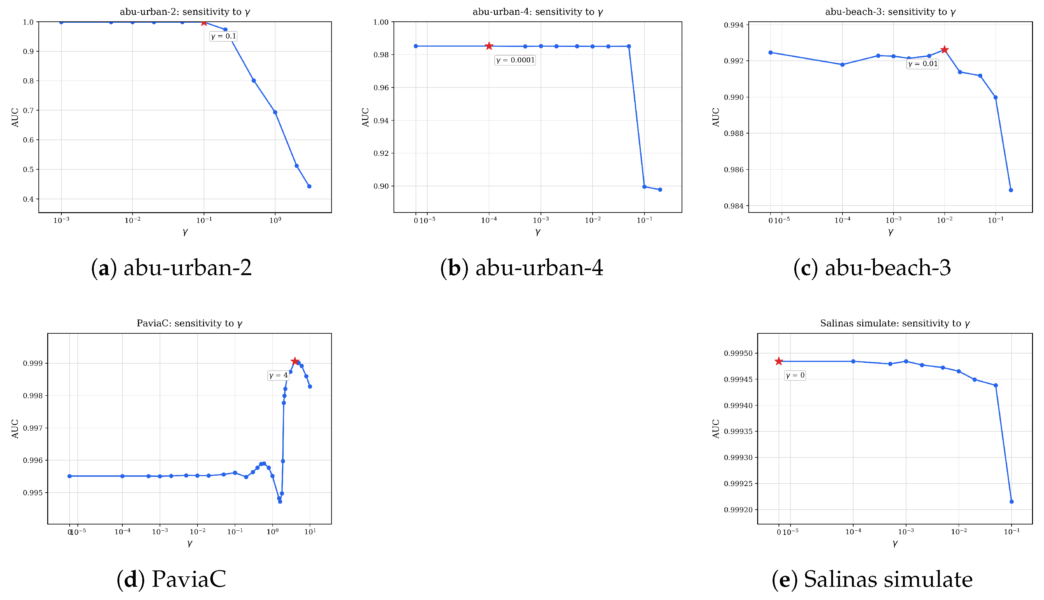
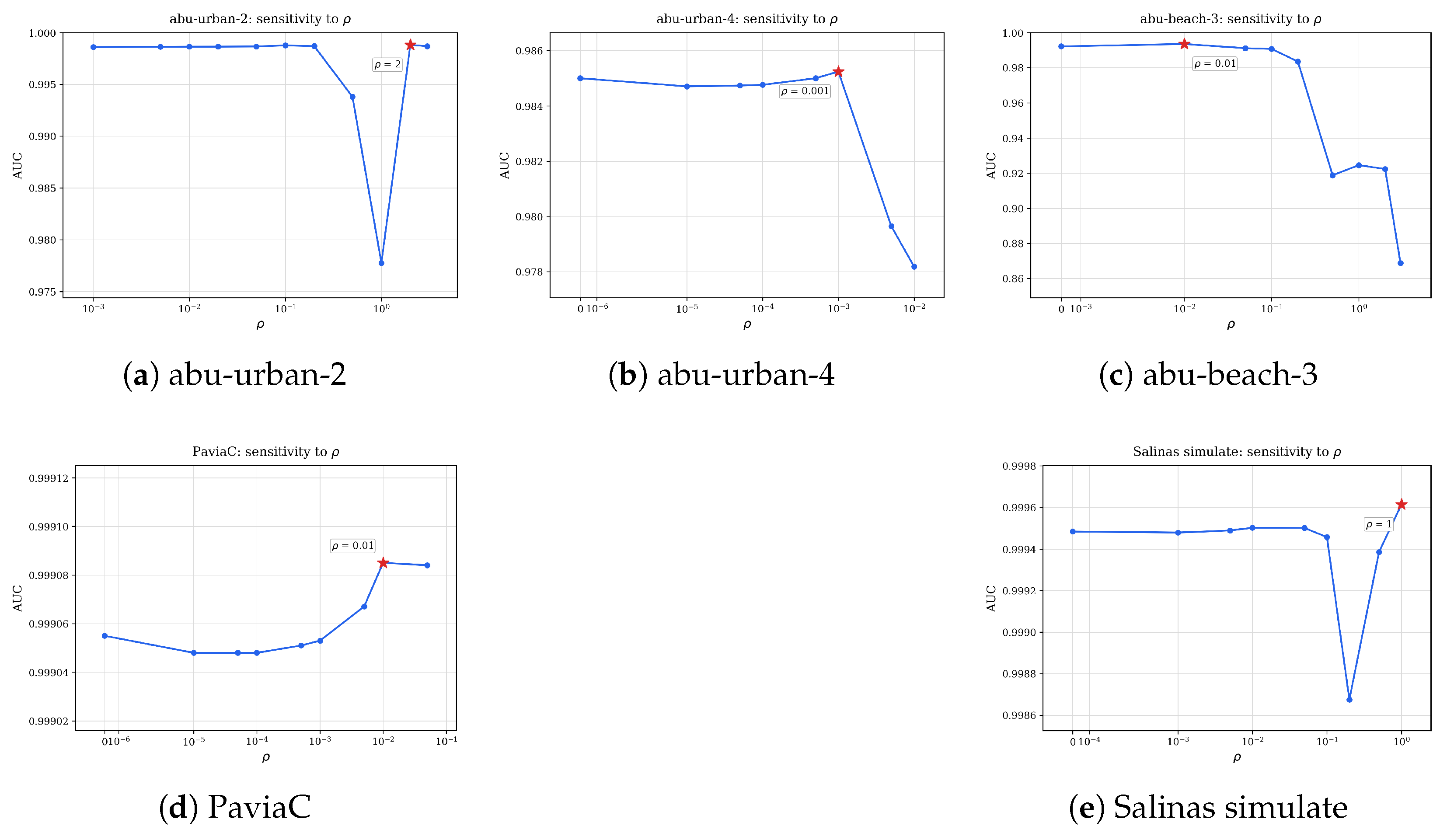
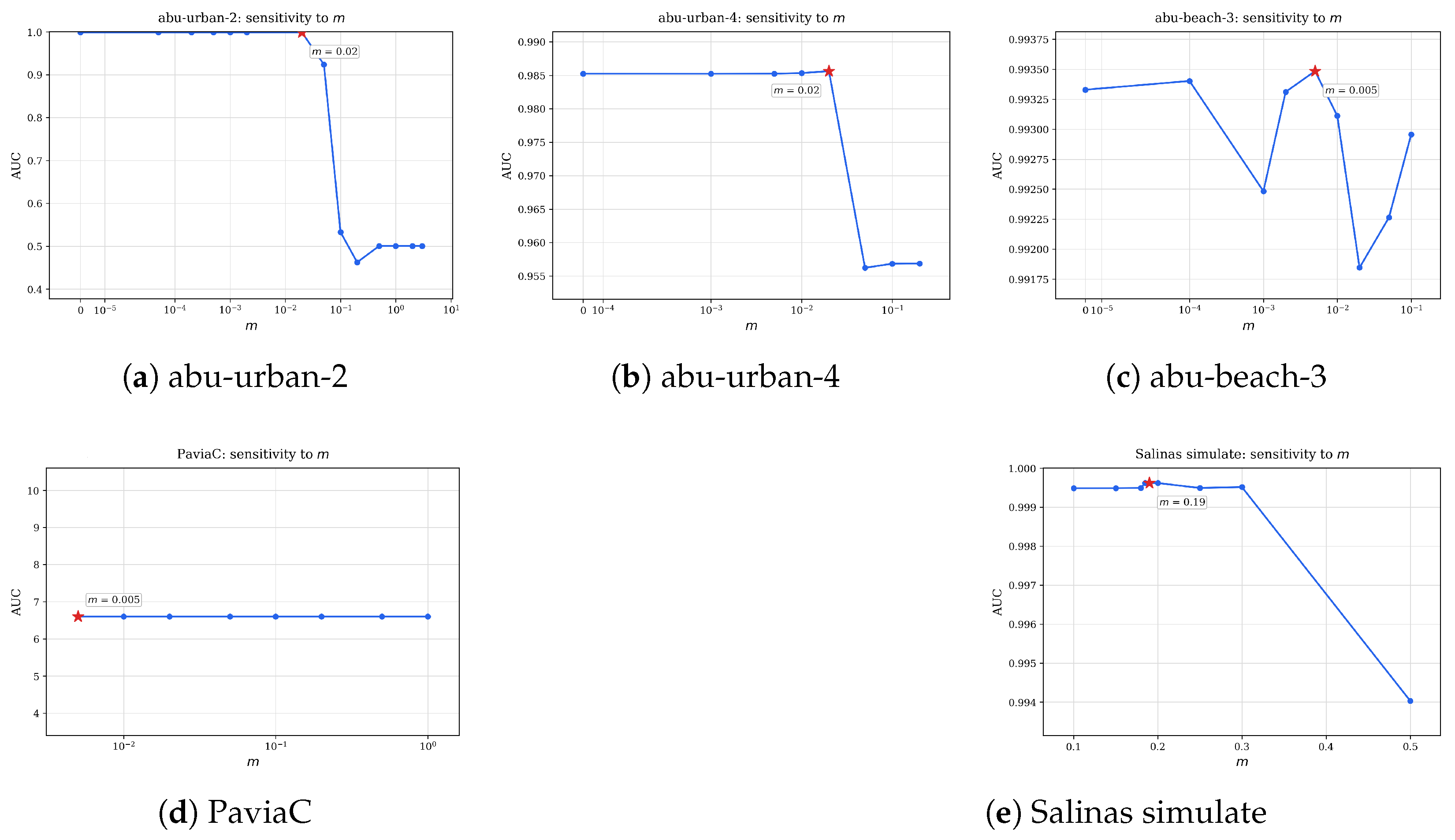
To assess the stability of HNGT-Net with respect to its key hyperparameters—the structural consistency weight $\beta$, the Laplacian response weight $\gamma$, the hard-negative separation weight $\rho$, and the response margin m—a systematic one-dimensional sensitivity analysis was conducted on each of the five benchmark datasets. In each sweep, one parameter was varied over a prescribed grid while all remaining hyperparameters were held fixed at their reference values. The resulting AUC curves are shown in Figure 5, Figure 6, Figure 7 and Figure 8, and the selected optimal values are summarized in

Table 7. Optimal hyperparameters selected for each benchmark dataset.

Dataset	β	γ	ρ	m
abu-urban-2	2	0.1	2	0.02
abu-urban-4	0.02	0.0001	0.001	0.02
abu-beach-3	0.01	0.01	0.01	0.005
PaviaC	1	4	0.01	0.005
Salinas simulate	0.001	0	1	0.185

.

Structural consistency weight $\beta$. Figure 5 plots the detection AUC as a function of $\beta$, which scales the edge-weight structural alignment term ${\mathcal{L}}_{\mathrm{struct}}$ in Equation (18). The five datasets exhibit markedly different sensitivity profiles. On abu-urban-2, the AUC increases steadily with $\beta$ and peaks at $\beta =2$ (AUC $=0.9985$); on abu-urban-4, the optimum is much smaller ($\beta =0.02$, AUC $=0.9851$); abu-beach-3 and PaviaC favor intermediate values of $\beta =0.01$ (AUC $=0.9925$) and $\beta =1$ (AUC $=0.9955$), respectively; while Salinas simulate achieves its best result at $\beta =0.001$ (AUC $=0.9995$). These disparities reflect the varying spatial homogeneity of the background scenes: urban scenes with heterogeneous human-made structures require stronger structural regularization, whereas agricultural or synthetic scenes with spectrally uniform backgrounds need only weak structural coupling.

Laplacian response weight $\gamma$. Figure 6 shows the sensitivity to $\gamma$, which balances the graph-Laplacian consistency term ${\mathcal{L}}_{\mathrm{lap}}$. On abu-urban-2, the AUC rises monotonically up to $\gamma =0.1$ (AUC $=0.9986$) before collapsing for $\gamma \ge 0.2$, indicating that a moderate Laplacian penalty is beneficial but excessive smoothing erases the fine spectral deviations associated with small targets. abu-urban-4 is almost insensitive to $\gamma$ in the range $[0,0.05]$, with a flat plateau near $0.9851$. abu-beach-3 peaks at $\gamma =0.01$ (AUC $=0.9926$), while PaviaC shows a pronounced upward trend that culminates at $\gamma =4$ (AUC $=0.9991$). Salinas simulate is entirely insensitive to $\gamma$ in the tested range, with its optimum at $\gamma =0$ (AUC $=0.9995$). This suggests that the value of high-order topological smoothing depends strongly on the spectral dimensionality and background complexity of the scene.

Hard-negative separation weight $\rho$. Figure 7 examines the influence of $\rho$, which scales the hinge separation loss ${\mathcal{L}}_{\mathrm{sep}}$. All datasets display a non-monotonic behavior: the AUC first improves as $\rho$ increases from zero, reaches a distinct maximum, and then degrades when the separation term dominates the total objective. The optimal $\rho$ values are $\rho =2$ for abu-urban-2 (AUC $=0.9988$), $\rho =0.001$ for abu-urban-4 (AUC $=0.9852$), $\rho =0.01$ for abu-beach-3 (AUC $=0.9935$), $\rho =0.01$ for PaviaC (AUC $=0.9991$), and $\rho =1$ for Salinas simulate (AUC $=0.9996$). The narrowness of the peak on abu-urban-4 underscores the need for careful tuning of the separation weight in scenes with subtle anomalies.

Response margin m. Figure 8 presents the sensitivity to the margin m that appears in the hinge separation loss Equation (17). For abu-urban-2, the AUC remains near $0.9988$ for $m\in [0,0.002]$, then jumps to its maximum at $m=0.02$ (AUC $=0.9989$), after which performance collapses precipitously for $m\ge 0.05$. A similar pattern is observed on abu-urban-4, where the optimum is also $m=0.02$ (AUC $=0.9856$). abu-beach-3 peaks at $m=0.005$ (AUC $=0.9935$), whereas PaviaC is completely flat at AUC $=0.9974$ for all tested margins, implying that the separation constraint is either inactive or always satisfied for this scene. Salinas simulate achieves its best AUC of $0.9996$ at $m=0.185$. The sharp transitions seen on the urban datasets confirm that the margin must be large enough to enforce a tangible gap between normal and hard-negative responses, yet small enough to avoid over-separating spectrally similar background pixels.

3.5. Ablation Study

To validate the incremental contribution of each learning objective, a cumulative ablation study was conducted by successively adding the four hyperparameter-weighted modules—structural consistency ($\beta$), Laplacian response consistency ($\gamma$), hard-negative separation ($\rho$), and response-margin separation (m)—on top of the node-level consistency baseline. In each step, the newly introduced module was set to its optimal value identified in the preceding hyperparameter sensitivity analysis, while all subsequent modules remained disabled (weight $=0$). The resulting progression is reported in

Table 8. Cumulative ablation study: detection AUC as each module is successively added to the node-consistency baseline. The baseline corresponds to the best node-only result ($\beta =\gamma =\rho =m=0$); subsequent columns show the AUC after enabling the optimal value of the indicated module while keeping all later modules at zero. For abu-urban-4, the baseline was obtained after a seed-diagnostic restart (see text). PaviaC did not include a dedicated margin search.

Dataset	Node Only	+β	+β + γ	+β + γ + ρ	+β + γ + ρ + m
abu-urban-2	0.9973	0.9985	0.9986	0.9988	0.9989
abu-urban-4	0.9850	0.9851	0.9851	0.9852	0.9856
abu-beach-3	0.9918	0.9925	0.9926	0.9935	0.9935
PaviaC	0.9923	0.9955	0.9959	0.9991	—
Salinas simulate	0.9995	0.9995	0.9995	0.9995	0.9996

.

Node-level baseline. The node-consistency term ${\mathcal{L}}_{\mathrm{node}}$ already achieves strong detection performance in isolation: its AUC ranges from $0.9850$ (abu-urban-4) to $0.9995$ (Salinas simulate). This confirms that the frozen-teacher paradigm provides a robust prior for normal-background representation even before any relational or discriminative regularization is introduced.

Structural consistency ($\beta$). Adding the edge-weight alignment term yields the largest single gain on PaviaC ($+0.0032$), where the scene’s heterogeneous human-made structures—buildings, roads, and water—benefit strongly from explicit pairwise similarity modeling. Moderate improvements are observed on abu-urban-2 ($+0.0012$) and abu-beach-3 ($+0.0007$). On abu-urban-4, the gain is small ($+0.0001$) because the successful training chain was already identified after a seed-diagnostic restart; nevertheless, structural consistency still contributes positively. On Salinas simulate, the baseline is near saturation, and the incremental contribution of ${\mathcal{L}}_{\mathrm{struct}}$ is minimal ($+0.0000$).

Laplacian response consistency ($\gamma$). The high-order topological smoothing term produces its strongest effect on PaviaC ($+0.0004$), complementing the structural term by regularizing graph-frequency responses in spectrally textured backgrounds. On abu-urban-2 and abu-beach-3, the gains are modest ($+0.0001$ each), while on abu-urban-4 and Salinas simulate the Laplacian term does not materially change the AUC. These results suggest that ${\mathcal{L}}_{\mathrm{lap}}$ is primarily helpful when the normal background exhibits pronounced spectral–spatial texture that cannot be fully captured by node and edge consistency alone.

Hard-negative separation ($\rho$). The separation hinge loss produces the largest cumulative ablation improvement on PaviaC ($+0.0032$) and abu-beach-3 ($+0.0009$). On PaviaC, the hard-negative term almost doubles the total gain accumulated up to that point, indicating that the bridge-structure anomalies are particularly well separated once an explicit normal–negative margin is enforced. On abu-beach-3, the large $\rho$ gain reflects the high spectral similarity between fishing-related targets and the sandy background, which the preceding consistency terms alone cannot fully disentangle. On abu-urban-2, the improvement is moderate ($+0.0002$), while on abu-urban-4 and Salinas simulate, the contribution is small ($+0.0001$ and $+0.0000$, respectively).

Response margin (m). The margin parameter yields a clear positive gain only on abu-urban-4 ($+0.0004$) and Salinas simulate ($+0.0001$). On abu-urban-2, the gain is marginal ($+0.0000$), and on abu-beach-3, the best margin configuration slightly underperforms the $\rho$-only result ($-0.0000$), suggesting that the hinge loss is already well-satisfied by the preceding separation term for this scene. PaviaC does not contain a dedicated margin search in the available log data, so no cumulative entry is reported; the final AUC for this dataset therefore equals the $\rho$-only result.

Summary. Taken together, the cumulative ablation results reveal a clear scene-dependent hierarchy of module importance. Structural consistency ($\beta$) and hard-negative separation ($\rho$) are the two primary drivers of performance: together they account for the majority of the total improvement on PaviaC ($+0.0064$ out of $+0.0068$), abu-urban-2 ($+0.0014$ out of $+0.0016$), and abu-beach-3 ($+0.0016$ out of $+0.0017$). Laplacian smoothing ($\gamma$) and the margin constraint (m) act as secondary refinements that become relevant only when the primary terms leave residual discrimination gaps. This modular behavior validates the design rationale of HNGT-Net: rather than relying on a single dominant objective, the framework layers complementary regularizers so that each scene can exploit the particular combination best suited to its background complexity and anomaly characteristics.

4. Discussion

The experimental results and ablation studies jointly indicate that HNGT-Net improves hyperspectral small-target detection through complementary representation and discrimination mechanisms. The topology-transfer objectives preserve normal-background information at node, relational, and graph-smoothness levels, whereas the hard-negative and response-margin terms explicitly enlarge the separation between normal samples and difficult normal-like perturbations. This division is supported by the ablation results: structural consistency ($\beta$) and hard-negative separation ($\rho$) provide the principal gains on several scenes, while Laplacian consistency ($\gamma$) and the margin term (m) provide additional refinements when residual discrimination ambiguity remains. Thus, the improvement cannot be attributed to a single loss component; it results from combining topology preservation with boundary-aware learning.

The cross-scene results also reveal that the contributions of the objectives are data dependent. Scenes with more informative local spectral–spatial relationships benefit from structural or Laplacian regularization, whereas excessive regularization can limit the flexibility of the compact student on other backgrounds. Accordingly, the loss weights and hard-negative parameters were selected sequentially for each dataset through one-factor-at-a-time sensitivity experiments, while keeping the remaining settings fixed. This procedure provides an interpretable basis for the reported settings and shows that a uniform hyperparameter configuration is not necessarily optimal for hyperspectral scenes with different background complexity and target contrast.

The efficiency results should be interpreted together with the detection results. The student branch substantially reduces the parameter burden relative to the teacher, whereas the complete teacher–student stack remains compact. This makes the approach suitable when high-quality anomaly scoring is required under restricted model capacity. At the same time, graph construction and teacher–student transfer are performed during training, so the main deployment advantage is the compactness of the learned student representation rather than the elimination of all offline computation.

Several limitations suggest directions for further research. First, the current hyperparameters are selected per scene and may require re-tuning when spectral resolution, background composition, or anomaly scale changes substantially. Second, projected-gradient hard negatives approximate difficult deviations from normal pixels but cannot represent every possible physical anomaly signature. Third, although the model is compact, scalable graph construction remains important for very large hyperspectral images. Future work will investigate adaptive parameter selection, more physically realistic hard-negative synthesis, and scalable graph-learning strategies for large-area and streaming hyperspectral data.

5. Conclusions

This paper has presented the Hard-Negative-Guided Topology Transfer Network (HNGT-Net), a lightweight teacher–student framework designed for hyperspectral small-target detection without any anomaly prior. Instead of relying on implicit background assumptions, HNGT-Net organizes pure normal pixels into a similarity graph that couples spatial adjacency with feature-space nearest neighbors, and then transfers the resulting spectral–spatial topology from a frozen teacher to a compact student through a three-level consistency objective over node embeddings, structural relations, and graph-Laplacian responses. To compensate for the complete absence of anomalous training data, hard negatives are synthesized directly on normal samples via sparsity-gated projected gradient perturbation, and a response-margin separation constraint compels the student to react to such negatives far more strongly than to normal pixels, which effectively alleviates distribution overfitting. Comprehensive evaluation on four public benchmark scenes and one Salinas-derived synthetic dataset shows that HNGT-Net attains a mean AUC of 0.9953 together with the smallest cross-dataset variance among all compared methods, indicating both high accuracy and stable generalization across diverse sensing scenes. Meanwhile, the student branch compresses its parameter count by 10.5× relative to the teacher; because the frozen teacher participates in inference, this result should be read as student-side compression within a complete stack of approximately 0.23 M parameters, which remains compact for resource-constrained remote sensing platforms.

The present results should be interpreted within the scene-specific normal-only protocol: each model is trained on a purified normal image derived from the same scene on which it is subsequently evaluated. Accordingly, the reported experiments do not establish cross-scene, cross-sensor, or cross-domain transfer. A strict evaluation in which training and testing scenes or sensors are fully separated, with no target-scene purification or adaptation, will be investigated in future work.

It is worth contrasting the proposed approach with recent spectral-guidance paradigms such as the Spectral Objectness Prior Module (SOPM) in SPG-OD [43], which achieves strong target-directed performance by explicitly exploiting known spectral signatures. HNGT-Net occupies a complementary niche: it is designed for scenarios where no target spectral prior exists, and it therefore learns anomaly discriminability indirectly through normal-topology transfer rather than through direct spectral targetness scoring. Future work may explore hybrid architectures that combine the generalization benefits of topology transfer with adaptive spectral priors learned from limited target exposure.

Several directions deserve further exploration. First, replacing the manually fixed spatial and feature neighborhoods with learnable, adaptive graph topology would improve the flexibility of the framework across heterogeneous scene types. Second, generative synthesis of hard negatives beyond gradient-based perturbation could further enrich the diversity of negative examples and sharpen the response margin. Third, extending HNGT-Net to incremental learning scenarios would allow the student to adapt continuously to evolving background patterns, a capability that is essential for long-term autonomous monitoring tasks.