Article

An Enhanced Nonlinear Grid Transformation Method for Weather Radar Echo Extrapolation

1
China Flight Test Establishment, Xi’an 710089, China
2
Laboratory of Cloud-Precipitation and Severe Storms (LACS), Institute of Atmospheric Physics, Chinese Academy of Sciences, Beijing 100029, China
3
College of Earth and Planetary Sciences, University of Chinese Academy of Sciences (UCAS), Beijing 100049, China
4
Civil Aircraft Flight Test Center of China (CAFTC), Xi’an 710026, China
5
Binzhou Meteorological Bureau, Binzhou 256612, China
*
Author to whom correspondence should be addressed.
Remote Sens. 2026, 18(17), 2865; https://doi.org/10.3390/rs18172865
Submission received: 6 July 2026 / Revised: 19 August 2026 / Accepted: 21 August 2026 / Published: 24 August 2026

Highlights

What are the main findings?
  • The newly developed enhanced nonlinear grid transformation (ENGT) method not only reflects the nonlinear transformation of the position and shape of radar echoes but also extrapolates the change in reflectivity intensity.
  • In a set of ideal and conceptual experiments, the ENGT method outperformed the traditional OF method and the previous NGT method in terms of echo position and intensity. In selected real cases, the ENGT method also showed potential.
What are the implications of the main findings?
  • The core of the new method is to solve a 3 × 9 transformation matrix using the least squares method based on a small number of radar echo images before the extrapolation start time. This makes the new method computationally inexpensive and potentially applicable to operational nowcasting.

Abstract

In this study, a method capable of simultaneously extrapolating the position, shape, and intensity of weather radar echoes is proposed. As the method is an improved version of the previously proposed nonlinear grid transformation (NGT) method, it is referred to as the enhanced NGT (ENGT) method. By extending the nonlinear transformation matrix to include radar reflectivity as the third dimension in addition to the grid coordinates X and Y, a 3 × 9 transformation matrix is used to describe the continuous spatial variation in the radar reflectivity field. The transformation matrix is solved using historical near-term data, enabling the extrapolation of subsequent time steps. In a set of ideal extrapolation experiments combining translation, temporal increments, and path variations, the ENGT method demonstrated better qualitative and conceptual performance than the NGT and traditional optical flow (OF) methods. In a real squall line case, the ENGT method could predict the overall movement direction of the cloud system synthesized by moving and emerging cells. In a real enhanced convective cloud cluster case, the ENGT method achieved higher scores because it generated stronger reflectivity. Although there are still mathematically unsolved and statistically insignificant problems, the ENGT method shows potential in predicting strong reflectivity, and the computational efficiency for a single weather radar is considerable.

1. Introduction

Weather radar echoes visually present the intensity, coverage, and movement of precipitating cloud systems. The obtained heavy precipitation information has critical applications in various fields, such as urban waterlogging control, flash flood warnings, and flight scheduling. The extrapolation of weather radar echoes is among the core aspects of short-term precipitation nowcasting [1]. Analyzing historical radar echo sequences to predict the evolution of precipitating cloud systems in the near term can provide key support for heavy precipitation warnings and is an important research direction in meteorological monitoring and forecasting.
Radar echo extrapolation methods can be divided into traditional numerical methods and modern deep learning methods. Traditional methods focus on explicit feature changes in radar imagery and statistical laws, mainly including cross-correlation methods based on motion vector estimation (such as the TREC algorithm) [2,3,4], optical flow methods (such as the Farneback algorithm) [5,6,7], and centroid tracking methods [8,9,10]. These methods typically achieve radar echo extrapolation by obtaining displacement vectors or vector fields, which are mathematically simple to implement. However, precipitating cloud systems may exhibit nonlinear localized processes, such as splitting, merging, generation, and dissipation, and the instantaneous movement direction of radar echoes may not align with their intensification and development direction. These complexities result in the actual evolution of radar echoes not satisfying the mathematical assumptions of traditional methods, potentially leading to limited extrapolation prediction performance. Additionally, the shape, boundaries, and intensity of precipitating cloud system radar echoes vary over time, making accurate tracking of each boundary point, corner point, or feature point difficult using general image processing algorithms.
To overcome the bottlenecks of traditional extrapolation, deep learning has become a major research direction because it can learn nonlinear spatiotemporal evolution directly from radar sequences. Rather than being represented by a single architecture, recent progress can be grouped into several thematic streams. Early convolutional and encoder–decoder networks, typically built upon U-Net-like structures, extract multiscale spatial features but often suffer from progressive smoothing and a loss of intense small-scale structures at longer lead times. The incorporation of polarimetric variables or refined loss functions has partially alleviated these issues, yet the fundamental trade-off between spatial fidelity and forecast range remains [11,12]. To better handle temporal continuity, recurrent spatiotemporal models with gated memory or trajectory-aware state transitions (e.g., ConvLSTM and its variants, PredRNN) have been introduced to improve the propagation of motion and intensity evolution; however, autoregressive error accumulation and high training costs still degrade performance beyond the first hour [13,14,15]. More recently, attention-, transformer-, and frequency-enhanced architectures have emerged to explicitly capture long-range spatial dependencies and multiscale interactions; representative frameworks such as NowcastNet and global-frequency synergy models have demonstrated improved skill for extreme precipitation and squall line cases, yet their sensitivity to data distribution and computational demands limit easy transfer across radar networks [16,17,18]. Generative approaches, including adversarial and diffusion-based models, offer a principled way to represent forecast uncertainty and can produce sharper, more realistic echo structures, as shown by the deep generative model of radar (DGMR) and subsequent variants, but they still face challenges in terms of calibration, stability, and pixel-wise consistency [19,20]. Overall, deep learning methods can outperform conventional extrapolation methods in selected regions and event types, but their advantages are highly contingent on data quality, model design, lead time, and verification criteria.
Even when data quality is disregarded, weather radar echo extrapolation still faces challenges. The sheer volume of weather radar data is enormous. Moreover, outside of the United States, publicly available weather radar data that can be downloaded are scarce, which limits consistent model comparisons and improvements. Notably, despite the continuous emergence of intelligent models and increasing computational power in recent years, a universal intelligent model for weather radar echo extrapolation remains lacking. Therefore, researchers have noted that, compared with persistently stacked data and the computational power of intelligent models, the continued exploration of simpler mathematical models for computation and application remains necessary.
Previously, Sun et al. proposed a nonlinear grid transformation (NGT) method [21], which can be considered a novel mathematical approach for weather radar echo extrapolation, or at least a prototype. This method involves modeling the evolution of continuous radar echo sequences as nonlinear transformations of grids and characterizing the deformation and movement of radar echoes by solving a 2 × 6 transformation matrix, thereby achieving radar echo extrapolation. In both idealized experiments and real convective cases containing convective lines, the NGT method outperforms traditional optical flow (OF) methods. However, a key limitation of the NGT method is its inability to predict radar echo intensity, meaning that the extrapolated radar echoes only exhibit changes in position and shape, while the overall radar reflectivity remains unchanged. On the one hand, this does not yet meet the requirements of short-term nowcasting for radar reflectivity prediction; on the other hand, users of radar echo extrapolation products may perceive prediction results with unchanged radar reflectivity as unreliable. These issues also need to be addressed by other traditional mathematical extrapolation methods.
This study introduces recent key improvements to the NGT method, hereafter referred to as the enhanced NGT (ENGT) method. Through enhancements to the transformation matrix and solution process, the ENGT method can simultaneously predict the deformation, displacement, and intensity changes in radar echoes through extrapolation. Section 2 provides a review of the NGT method and details how to develop the ENGT method. Section 3 presents idealized and real case experiments. Section 4 discusses other known issues and limitations. Finally, Section 5 concludes this study.

2. Method

2.1. Review of the NGT Method and Its Principles

In the NGT method, a 2 × 6 transformation matrix is used to characterize the following nonlinear grid transformation:
[ X 2 , Y 2 ] T   =   M 2 × 6 [ X 1 , Y 1 , X 1 Y 1 , X 1 2 , Y 1 2 , 1 ] T
where X1 and Y1 are the uniform grid points of the radar echo before transformation and X2 and Y2 are the transformed grid points, which are typically nonuniform. This transformation is inspired by the fundamental affine transformations in computer graphics but incorporates nonlinear terms in X and Y. The transformation not only represents traditional transformations, such as translation, shearing, and rotation, but also achieves convex or concave shape changes along one side of the image, thereby capturing richer variations in precipitation radar echoes (e.g., the formation of bow-shaped echoes in a squall line). More intuitively, the transformation matrix obtained by the NGT method is characterized by continuous warping of the radar reflectivity field. By extrapolating this continuous transformation from historical data preceding the target time, the method enables the prediction of future radar imagery.
A more specific concept is illustrated in Figure 1, which is derived from a real and typical squall line event [21]. During this event, storm cells move northeastward along the low-level winds (e.g., 700 hPa winds), whereas new cells appear continuously on the right side of the southern part of the cloud system under the lower-level southerly inflow, forming a typical right-shift storm mechanism. As a result, the development direction (or visual movement direction) of the entire cloud system is east–northward, which differs from the instantaneous movement direction of cells. Under this mechanism, the entire cloud echo gradually forms the shape of a bow. By inputting adjacent continuous historical data, the NGT method can internally model and reproduce this overall change through nonlinear mesh transformation. The final prediction effect is that the NGT method stretches and distorts the entire image in the composite direction of moving and emerging cells rather than predicting the movement or birth of each individual cell.
The key to the NGT method is to solve M2×6 in Equation (1). This differs from traditional computer graphics approaches. With respect to general imagery, by identifying boundary points and corner points of features in an image, it is easy to obtain X and Y before and after transformations, thereby solving the transformation matrix through linear equations. However, the shape and local intensity of precipitation echoes are variable, and individual cells undergo merging and splitting, making accurate identification of multiple corresponding sets of X1, Y1, X2, and Y2 for the same target in adjacent images difficult. The NGT method does not search for specific points in the image but instead defines the following cost function and the estimated values used:
J   = Σ Q 1   Q 2 * 2
Q 2 *     Q 2 + Q 2 x X 2   X 1 + Q 2 y Y 2   Y 1
where J is the minimized cost function, which characterizes the minimal difference between Q1 transformed from (X1, Y1) to (X2, Y2) and the estimated value of Q2 at (X2, Y2), which is equivalent to one image being similar to the next after a transformation. Here, the summation Σ covers all data points whose reflectivity values have changed between the adjacent images at two times within the input historical data. A more specific example of valid samples is presented at the end of Section 2.2.1. Q1 is the intensity of the first radar echo, with coordinates on a uniform grid (X1, Y1); Q2 is the intensity of the second echo, with coordinates still on a uniform grid (X1, Y1); and Q2* is the estimated value of the second echo on the nonuniform grid (X2, Y2) after transformation by M2×6, characterized by a simplified first-order Taylor expansion of Q2. The estimation formula for Q2* is presented because the Q1 values after transformation by M2×6 are located at (X2, Y2). Equation (3) acts as a simple interpolation operator but requires the grid spacing to be larger than the target’s displacement per time step; a more specific operational description is provided in Section 2.2.4. Afterward, when Equation (1) is expanded into equations for X2 and Y2 and Equation (3) is substituted, the minimization objective of Equation (2) is equivalent to solving the following system of linear equations:
B   M * =   Q 2 x X 1   + Q 2 y Y 1     Q 2   +   Q 1
where
B = Q 2 x X 1 ,   Q 2 x Y 1 ,   Q 2 x X 1 Y 1 ,   Q 2 x X 1 2 ,   Q 2 x Y 1 2 ,   Q 2 x , Q 2 y X 1 ,   Q 2 y Y 1 ,   Q 2 y X 1 Y 1 ,   Q 2 y X 1 2 ,   Q 2 y Y 1 2 ,   Q 2 y
M * = m 1 , 1 ,   m 1 , 2 ,   m 1 , 3 ,   m 1 , 4 ,   m 1 , 5 ,   m 1 , 6 ,   m 2 , 1 ,   m 2 , 2 ,   m 2 , 3 ,   m 2 , 4 ,   m 2 , 5 ,   m 2 , 6 T
Using several consecutive historical radar reflectivity images preceding the forecast, the equations generated from valid grid samples in adjacent image pairs are assembled into a single system based on Equation (4). The least squares method is used to estimate M*, and finally, M2×6 can be obtained by reshaping the solution into the transformation matrix.

2.2. ENGT Method

2.2.1. Extended Transformation Matrix and Initial Solution

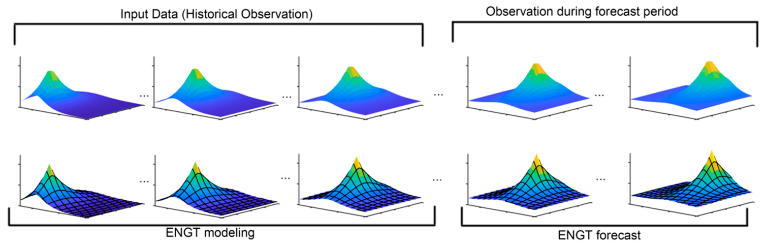
The NGT method cannot extrapolate radar reflectivity because it only transforms within the two-dimensional space of X and Y. By treating radar reflectivity as a third dimension and incorporating it into the transformation, the method can be used to simultaneously extrapolate both the spatial distribution and intensity of the radar reflectivity field. More generally, unlike the NGT method (Figure 1), the radar reflectivity surface in this case not only shifts and warps horizontally but also changes vertically (Figure 2).
To achieve this, a transformation matrix and a transformation formulation incorporating Z are proposed:
[ X 2 , Y 2 , Z 2 * ] T   =   M 3 × 9 [ X 1 , Y 1 , X 1 Y 1 , X 1 2 , Y 1 2 , 1 , X 1 Q 1 , Y 1 Q 1 , Q 1 ] T
Compared with Equation (1), the transformation matrix is 3 × 9, incorporating the pretransformation Q1 term and its nonlinear terms multiplied by the grid coordinates. Similar to the summation range of Equation (2), the minimized cost function becomes the following:
J = Σ Z 2 * Q 2 * 2
That is, after it is transformed to (X2, Y2), where the intensity of Q1 becomes Z2* for the nonuniform grid, the estimated difference with Q2 at (X2, Y2) is minimized. Expanding Equation (7) yields the following:
X 2   =   m 1 , 1 X 1   +   m 1 , 2 Y 1   +   m 1 , 3 X 1 Y 1   +   m 1 , 4 X 1 2   +   m 1 , 5 Y 1 2   +   m 1 , 6   +   m 1 , 7 X 1 Q 1   +   m 1 , 8 Y 1 Q 1   +   m 1 , 9 Q 1
Y 2 = m 2 , 1 X 1 + m 2 , 2 Y 1 +   m 2 , 3 X 1 Y 1 + m 2 , 4 X 1 2 + m 2 , 5 Y 1 2 + m 2 , 6 +   m 2 , 7 X 1 Q 1 +   m 2 , 8 Y 1 Q 1 + m 2 , 9 Q 1
Z 2 * = m 3 , 1 X 1 + m 3 , 2 Y 1 + m 3 , 3 X 1 Y 1 +   m 3 , 4 X 1 2 + m 3 , 5 Y 1 2 + m 3 , 6 + m 3 , 7 X 1 Q 1 + m 3 , 8 Y 1 Q 1 +   m 3 , 9 Q 1
Substituting Equations (9)–(11) into Equations (3) and (8) ultimately reduces to the following system of linear equations to be solved:
B   M * =   C
where C is the constant term, B is a known coefficient matrix, and M* is an array of coefficients to be solved. The forms of C, B, and M* are as follows:
C   =   Q 2 x X 1   +   Q 2 y Y 1 Q 2
B = Q 2 x X 1 ,   Q 2 x Y 1 ,   Q 2 x X 1 Y 1 ,   Q 2 x X 1 2 ,   Q 2 x Y 1 2 ,   Q 2 x , Q 2 x X 1 Q 1 , Q 2 x Y 1 Q 1 , Q 2 x Q 1 , Q 2 y X 1 ,   Q 2 y Y 1 ,   Q 2 y X 1 Y 1 ,   Q 2 y X 1 2 ,   Q 2 y Y 1 2 ,   Q 2 y , Q 2 y X 1 Q 1 , Q 2 y Y 1 Q 1 , Q 2 y Q 1 , - X 1 ,   - Y 1 ,   - X 1 Y 1 ,   - X 1 2 ,   - Y 1 2 ,   - 1 , - X 1 Q 1 , - Y 1 Q 1 , - Q 1
M * = m 1 , 1 ,   . . .   m 1 , 9 , m 2 , 1 ,   . . .   m 2 , 9 , m 3 , 1 ,   . . .   m 3 , 9   T
Similar to the NGT method, the initial value of M3×9 is obtained by solving M* through the least squares method and arranging the resulting coefficients accordingly.
More specifically, B is a matrix with 27 columns and Nsample rows, and C is an array with Nsample rows, where Nsample represents the number of samples. The sample selection principle involves choosing data points where “Q2Q1 ≠ 0” and values are non-NaN. The images of adjacent times are sequentially treated as Q1 and Q2. For example, for the images of 10 consecutive historical times, the first image is taken as Q1, and the second image is taken as Q2. The qualified data points are enumerated, Nsample is accumulated, and the rows of B and C are expanded. The second image is then taken as Q1, and the third image is taken as Q2 to expand the linear equations represented by Equation (12). The ninth image is taken as Q1, and the tenth image is taken as Q2. Note that the number of samples selected for each enumeration of adjacent image times may differ, and the size of the final equation set is not as large as the full size of the image multiplied by the number of historical times because data points are selected only when the image value (radar reflectivity value) changes in the adjacent time. In addition, if the final Nsample is fewer than 27, it indicates that there is almost no precipitation echo and that the equations have changed from overdetermined to underdetermined; in this case, the solution and extrapolation are abandoned. The above rules for listing the contents of each row of B and C help prevent the equations from becoming unsolvable, since these rules can prevent situations where the equations contain a large number of zero values or identical equations.

2.2.2. Further Iterative Solving

Compared with the NGT method, the ENGT method introduces additional quadratic nonlinear terms, which may amplify errors during the estimation of M3×9 and extrapolation. One source of error is evidently the first-order Taylor expansion shown in Equation (3). However, if a second-order Taylor expansion is directly applied to the binary variables X and Y, quadratic terms of the elements in M3×9 would arise, making it difficult to derive a simple solvable form in subsequent steps. Below, an iterative solution method that accounts for the second-order Taylor expansion in Equation (3) is introduced. While theoretical convergence cannot yet be proven in this study, it has been found to be practically feasible. After the initial value of M3×9 in the previous step is obtained, X2 and Y2 can be derived on the basis of Equation (7). The initial values of ΔX and ΔY are then calculated from their differences with X1 and Y1. The iteration process is as follows:
C ( i t e r = 2 )   =   C ( i t e r = 1 ) α 0.5 2 Q 2 x 2 Δ X   ( i t e r = 1 ) 2 + 0.5 2 Q 2 y 2 Δ Y   ( i t e r = 1 ) 2 + 2 Q 2 x y Δ X   ( i t e r = 1 ) Δ Y   ( i t e r = 1 )
M * ( i t e r = 2 ) = Regress B ,   C ( i t e r = 2 )
Δ X   ( i t e r = 2 ) = X 2 ( i t e r = 2 ) X 1
Δ Y   ( i t e r = 2 ) = Y 2 ( i t e r = 2 ) Y 1
Here, the superscripts (iter = 1) and (iter = 2) represent the previous iteration value and the current calculated value, respectively. α is set to 0.5 here, making the solution akin to a relaxed iterative approach. Each iteration updates the values of C, M*, ΔX, and ΔY, with the core objective of solving for a more accurate M*. The findings of this study show that the results typically stabilize within 3 iterations. The rule to terminate the iteration is when the residual sum of squares of multiple linear regression in Equation (17) is less than 10−7, which is usually achieved in 10 iteration steps. The specific calculation of this index, the influence of different α values, and the convergence of the above iterative scheme are introduced in Section 3.1.2.

2.2.3. Backward Time Interpolation for Radar Echo Extrapolation

After M3×9 is obtained, some challenges remain in acquiring extrapolated radar echoes. If direct forward extrapolation is performed using Equation (7), the resulting grid is nonuniform, which is not conducive to quantitative applications, such as quickly locating points at specified positions. If the nonuniform grid is resampled into a uniform grid, for 600 × 600 grid points or larger-sized images, the computational time required for resampling may significantly exceed that of the ENGT method itself, leading to inefficient computation. On the other hand, regardless of whether forward or backward extrapolation is performed using Equation (7), errors accumulate nonlinearly. Below, a practical method is presented. First, after M3×9 is obtained, the initial forecast time Q1 is substituted into Equation (7) to calculate the extrapolated values of one step (X2, Y2, and Z2*), and the grid transformation vector field for an individual time step is computed as follows:
U * =   X 2 X 1
V * = Y 2 Y 1
W * = Z 2 * Q 1
U* and V* characterize how many grid units the grid moves per time step, and W* represents the local rate of change in the variable values in the image per time step. Afterward, temporal backward interpolation is performed according to the following steps:
(a)
U* and V* are subtracted from X1 and Y1, respectively, which is the backward extrapolation of X and Y for a single time step, resulting in the newly obtained Xnew and Ynew.
(b)
U*, V*, and W* at Xnew and Ynew are estimated using bilinear interpolation.
(c)
Using bilinear interpolation, Q1 is estimated at the location (Xnew, Ynew), and W* is subsequently added to obtain the uniform grid radar echo image extrapolated by one step.
(d)
The extrapolation is started for the next time step. At this point, U* and V* are subtracted from the previous step’s Xnew and Ynew to obtain the updated Xnew and Ynew, respectively.
(e)
The W* field obtained at each time step is accumulated. For cases where the extrapolation exceeds one time step, Q1 is estimated at the location (Xnew, Ynew), and then the accumulated W* field is added to obtain the extrapolated uniform grid radar echo image.
(f)
Steps (d) and (e) are repeated to achieve extrapolation over multiple time steps.

2.2.4. Summary of the Steps of ENGT and Supplementary Instructions

(a)
For real cases, composite reflectivity or constant-altitude plan position indicator (CAPPI) data are first interpolated to a uniform horizontal grid. The resulting radar reflectivity field is then spatially downsampled before the ENGT algorithm is applied. For example, an image with a horizontal resolution of 1 km × 1 km and dimensions of 600 × 600 is reduced to a coarse grid with a horizontal resolution of 10 km × 10 km and dimensions of 60 × 60 by spatial averaging. This ensures that the grid spacing exceeds the displacement of the radar echoes between successive radar scans. For instance, at a translation speed of 20 m s−1, which is a common high wind speed in the middle and lower levels of the troposphere, and a radar volume scan data interval of 4 to 6 min, the cloud object moves 4.8~7.2 km. In this case, a grid spacing of 10 km satisfies the ENGT solution criteria.
(b)
All variables involved in the calculation are converted to at least double precision. This is because three elements multiply together to compose some terms of matrix B. When each element of these terms changes by two orders of magnitude, the amplitude of change after multiplication can reach six orders of magnitude. At this time, there is no residual accuracy for subsequent calculations under single precision. This also makes the normalization of variables by scaling unnecessary, since even scaling cannot solve the equations with single precision. In addition, the consistency of the X and Y units in each calculation step should be ensured. For example, when the input X and Y are the distances relative to the radar (or latitude and longitude), all subsequent X and Y values involved in the calculation must be the same defined distance (or latitude and longitude).
(c)
A two-dimensional Gaussian filter with a radius of 10 grid points and a standard deviation of 1 grid point is applied to the coarse grid imagery. This is because the ENGT method does not use detailed textures, and smoothed images better align with the conditions derived from the method.
(d)
The initial value of M3×9 is calculated using the method described in Section 2.2.1.
(e)
The final value of M3×9 is determined using the method outlined in Section 2.2.2.
(f)
For real cases, the transformation vector field (U*, V*, and W*) is calculated on the basis of the downsampled, Gaussian-filtered images using Equations (20)–(22).
(g)
For real cases, the U*, V*, and W* fields obtained from the previous step are interpolated onto the original fine grid. Afterward, the method described in Section 2.2.3 is applied to the original fine-resolution radar reflectivity field to produce the extrapolated radar reflectivity field on the fine uniform grid.
Moreover, the standard deviation of one grid point in step (c) above is used to further ensure the reliability of the spatial derivatives within one grid distance around a grid point. This not only helps solve the system to satisfy the Taylor expansion approximation in Equation (13) but also makes it easier to use a simpler method (e.g., central difference) instead of a multipoint difference when the spatial derivative is solved. Omitting the two-dimensional Gaussian filtering here may yield an obviously unsatisfactory result, since the coarse grid points that are reduced only by spatial averaging have difficulty providing a continuous and smooth spatial derivative. In contrast, when this standard deviation is set to be larger, it is equivalent to the information being diluted and further reduced in dimension, decreasing the reliability of the image change characteristics. The 10 grid radius in step (c) above is not very important in most cases because the weighting coefficients of the grid values outside the two standard deviations are very small during filtering. The main function of such a radius is to smooth scattered convection, reduce the mutability of the spatial derivative, and connect scattered clouds with adjacent cloud systems to produce a smoother spatial derivative. Sensitivity experiments on the above parameters can be found in the Supplementary Materials.

2.3. Experimental Setup and Comparison Methods

2.3.1. Cases and Data for Experiments

In Section 3, ideal and real experiments are conducted to evaluate the extrapolation performance. In ideal experiments, following the approach for the NGT method [21], a two-dimensional Gaussian field was generated with prescribed translations, echo growth and decay, and different motion trajectories to create idealized test cases for qualitatively evaluating the performance of the ENGT method. The specific settings of the input and target samples are shown in Appendix A and the Supplementary Materials.
In real experiments, the cases and data used are briefly described as follows:
(1) Cloud System with Convective Lines
Real case 1 is a typical squall line event [22] that occurred on May 20, 2011, over the southern U.S., which was also used in the original NGT study [21]. As mentioned in Section 2.1, the overall echo shape of the squall line cloud system shows typical right-moving storm characteristics and bow shape changes, which are used to test whether an extrapolation method can properly predict these typical cloud development directions and overall shape changes. The S-band NEXRAD radar in Oklahoma, U.S., with the site code KTLX (located at 97.28°W, 35.33°N) is used. A volume scan consisting of 15 elevations is observed approximately every 4 min. Triple linear interpolation [23] in polar coordinates (elevation, azimuth, and radial distance) is used to calculate the CAPPI at a height of 3 km above the radar origin from the volume scan data. The resolution is 1 km × 1 km, and the size of a single CAPPI is 600 × 600. Compared with composite reflectivity, the 3 km height CAPPI contains little clutter in the boundary layer and ground occlusion, which greatly reduces interference factors in an extrapolation experiment.
(2) Convective Cloud Clusters Developing from Weak Radar Echoes
Real case 2 is a convective weather event that occurred on 11 July 2023, in northern Ningxia Province, China. This case is used to test whether an extrapolation method can properly predict the movement of a group of convective clouds and the increase in reflectivity at the same time. The radar data are a radar mosaic product of composite reflectivity, which is produced and provided by the China Meteorological Administration. The production method of this data product is not fully disclosed, but it is believed that the signal-to-noise ratio is used to shield some non-precipitation echoes and that known ground objects and clutter are premasked. Although most of the clutter is eliminated, sometimes there is still a small amount of non-precipitation echo residual in the boundary layer in this product. This data product has a 1 km × 1 km resolution and is produced every 6 min. The ranges from 103 to 109°E and from 35 to 41°N are selected in this case, and the size of a single composite reflectivity image is 600 × 600.
(3) Isolated Hailstorm
Real case 3 is an isolated hailstorm event that occurred on 9 July 2023 in Tengzhou, Shandong Province, China. This case is selected because hail from isolated cells is also a noteworthy hazard in severe convective weather monitoring; however, prediction may be more challenging because of the lack of a clear mother cloud system to provide an overall change trend. The S-band CINRAD radar with site code Z9516 (located at 117.2°E, 34.3°N) is used. A volume scan consisting of 9 elevations is observed approximately every 6 min. More information about this type of radar can be found in [24]. The 3 km height CAPPI is derived from the original volume scan data via the same approach as previously mentioned in real case 1. The resolution is 1 km × 1 km. The size of a single CAPPI is initially 600 × 600; then, an area with a size of 200 × 200 and a range of 200 km × 200 km centered on the hail area is selected as a supplementary experiment.
(4) Overall statistics of 22 precipitation events
In addition to the demonstration of typical cases, more samples are needed to test whether the advantages of ENGT are statistically significant. Experiments similar to those in real case 2 but centered in Shaanxi Province (106~112°E, 32~38°N), China, were carried out with 22 precipitation events and 3069 h of data. The time span is from May 2024 to August 2024. The source, resolution and grid number of the input composite reflectivity images are the same as those in real case 2.
In addition, the logarithmic unit dBZ is used for all the above radar reflectivity values, including the original data and the images used for extrapolation, and there is no calculation step that converts a reflectivity value to a linear unit.

2.3.2. Comparison Methods

The methods involved for comparison can be divided into the following categories:
(1) NGT and OF
To fairly evaluate the improvement in the ENGT method relative to the NGT method, a consistent NGT and OF calculation scheme is adopted and proposed for NGT, as shown in [21]. Here, the OF scheme takes the data at the beginning of extrapolation and the previous adjacent time step as inputs. As with the NGT and ENGT methods, spatial averaging is used to obtain data with a spatial resolution of 10 km × 10 km for the OF scheme, but two-dimensional Gaussian filtering is not performed. The displacement vector field is interpolated back to the 1 km × 1 km grid after it is obtained by the OF scheme. In addition, the input data for the NGT and ENGT methods are within 1 h before the start of extrapolation, with 14 images for real case 1 and 10 images for real cases 2 and 3, respectively. A 1 h extrapolation experiment is carried out, and the difference in the time steps is the same as previously mentioned.
(2) Schemes of Enhanced-OF
Considering that the OF method mentioned above is considered to be the simplest OF scheme, it inputs less information than the NGT and ENGT methods do, and some studies have proposed enhanced-OF schemes based on multiple temporal and spatial scales [5]. However, an enhanced-OF scheme inevitably involves many additional parameters, which introduce uncertainty to the experiment. Two relatively clear enhanced-OF schemes are designed below. The first enhancement scheme involves repeating the simplest OF scheme at two adjacent times, one hour before extrapolation, and, finally, time-averaging the obtained displacement vector field, which is called the OF-E1 scheme. The second enhancement scheme includes the average of four displacement vector fields: (a) the simplest OF scheme; (b) the OF scheme that is carried out on a 20 km × 20 km grid with two data points at the beginning of extrapolation and two times earlier as input; (c) the OF scheme that is carried out on a 50 km × 50 km grid with two data points at the beginning of extrapolation and 30 min earlier as input; and (d) the OF scheme that is carried out on a 100 km × 100 km grid with two data points at the beginning of extrapolation and 60 min earlier as input. When the solution of the largest scale is not feasible (e.g., fewer than 3 grids per row or column), the solution is ignored, and the other three displacement vector fields are averaged. This scheme, which combines multiple temporal and spatial scales, is called the OF-E2 scheme.
In terms of the length of historical data used, the OF-E1 and OF-E2 methods are also based on historical 1 h data, which is the same as the ENGT and NGT methods to ensure that the amount of input information is consistent or at least similar. More specifically, the OF-E1 method uses exactly the same number of images as the ENGT and NGT methods do (e.g., 14 images for real case 1 and 10 images for real cases 2 and 3); the OF-E2 method uses four time and space scales, so the input data only has five images, but the maximum time span is still 1 h.
Notably, the OF-E1 and OF-E2 methods may not achieve better results than the simplest OF scheme for targets with features that are too simple. Therefore, the OF-E1 and OF-E2 methods schemes are not used for the ideal experiment, but an analysis of the causes is included in Section 3.1.1.
(3) Eulerian Persistence
Eulerian persistence is a method of evaluation that is often used as a baseline along with the OF method [25]. Most simply, it copies the image at the beginning of the extrapolation moment to the target moment without making any changes and calculates the skill score. The skill score of an extrapolation method needs to be better than the score obtained by Eulerian persistence; otherwise, it represents a trend error in the prediction of position and intensity because it is worse than inaction. This comparison method is also called the static reference when the NGT method was proposed [21]. The scheme is abbreviated as PB below.
It should also be noted that several other methods can be used as baselines. For example, simple advection [6] is based on a single vector, but its solution may be affected by echo center jumps and Lagrangian persistence and spectral prognosis (known as S-PROG) [26,27], but the calculation is relatively complex. As an extension of simple advection, the middle- and low-level wind fields from numerical weather prediction can also be used as a vector field for extrapolation, but the effect in the selected cases is not better than that in the above OF schemes. Considering the limited space and the need to focus on the characteristics of the ENGT method, no additional baseline solutions are examined in this study.

2.3.3. Statistics

The statistics used in real experiments can be divided into the following categories:
(1) Basic skill scores
To qualitatively evaluate the extrapolation results of the radar reflectivity field at the target times, commonly used accuracy metrics, such as the critical success index (CSI, also known as the threat score), the probability of detection (POD), and the false alarm ratio (FAR), are computed. The formulas for calculating these skill scores are as follows:
CSI   =   N A N A   +   N B   +   N C
POD = N A N A   + N C
FAR = N B N A + N B
where NA is the number of grid points where both the observed value and the extrapolated prediction exceed the specified threshold at the target time, i.e., the hit count; NB is the number of grid points where the extrapolated prediction exceeds the specified threshold but the observed value does not, i.e., the false alarm count; and NC is the number of grid points where the observed value exceeds the specified threshold but the extrapolated prediction does not, i.e., the miss count. The obtained CSI is the main reference, while POD and FAR are used for further explanation. For example, a high POD indicates a high prediction hit rate, but a high FAR at the same time indicates many false alarms, which also leads to a low CSI.
Three discrete integer thresholds of 20, 30, and 40 dBZ were selected as representatives in the calculations of the CSI, POD, and FAR. Weaker radar reflectivity (e.g., 10 dBZ) usually corresponds to drizzle or non-precipitation echoes and is less commonly used in such statistics. Stronger radar reflectivity (e.g., 50 dBZ) is usually the core of heavy precipitation or convection, which has a small area ratio across a wide range and may change rapidly or jump.
The above statistics are based on uniformly gridded CAPPI or composite reflectivity data (equidistant or equal latitude/longitude) with a horizontal resolution of 1 km × 1 km and are calculated using precise “point-to-point” statistical methods. Notably, for non-widespread echoes, the CSI and POD obtained at such fine resolution may be relatively small, as convective cells with diameters on the order of several kilometers exhibit uneven spatial distributions and rapid movement and evolution. Slight positional deviations in the extrapolated predictions can lead to a lower NA. However, this does not hinder comparisons between the different methods. Matching on a nearby range or coarser grids can alleviate the above problem and may increase the skill score. However, to avoid the arbitrariness of setting the resolution, a 1 km × 1 km grid is still used to calculate the CSI, POD, and FAR, and the fractions skill score, which can address the above problems, is introduced below.
(2) Fractions skill score
The fractions skill score (FSS) [28,29] can be regarded as an enhanced skill score. The FSS is calculated by traversing rectangular subregions of a certain area so that the problem of low CSI and POD caused by the slight misalignment of observations and predictions can be overcome. The FSS has many almost equivalent forms of calculation, and the simplest one [29] is provided as follows:
FSS ( n )   =   i = 1 N X j = 1 N Y 2 f n i j · o n i j i = 1 N X j = 1 N Y f n i j 2 + o n i j 2
where n is the number of grid points of the radius of the rectangular subregion to be traversed; otherwise, the side length of the rectangular subregion is 2n + 1. For example, when n = 2, for 1 km × 1 km grids, the side length of the rectangular subregion is 5 km. NX and NY are the numbers of grid points of the image in the X and Y directions, respectively. f (or o) is the fraction of the predicted (or observed) values in each rectangular subregion greater than a given threshold. In the following calculation of the FSS, as with the CSI, reflectivities of 20, 30, and 40 dBZ are taken as the threshold, and n is 2 and 5.
(3) Error statistics
The commonly used error statistics include the mean absolute error (MAE), root mean square error (RMSE), correlation coefficient (CC), and mean bias (MBias). Their calculation methods are as follows:
MAE   =   Z f o r e c a s t Z o b s ¯
RMSE = Z f o r e c a s t Z o b s 2 ¯
CC = Cov Z f o r e c a s t ,     Z o b s Std Z f o r e c a s t · Std Z o b s
MBias = Z f o r e c a s t Z o b s ¯
where Zforecast and Zobs are the predicted and observed radar reflectivity fields, respectively, at the grid points. For grid points less than 0 or with no value, they are set to 0. The superscript horizontal line represents the average of the content below the horizontal line within the range of all grid points. Cov and Std represent the covariance and standard deviation, respectively. Generally, the MAE and RMSE are used to measure the absolute degree of error, the CC is used to measure the similarity between two images, and the MBias is used to characterize the positive and negative bias of the prediction.

3. Results

3.1. Ideal Experiments

3.1.1. Comparison of Different Methods

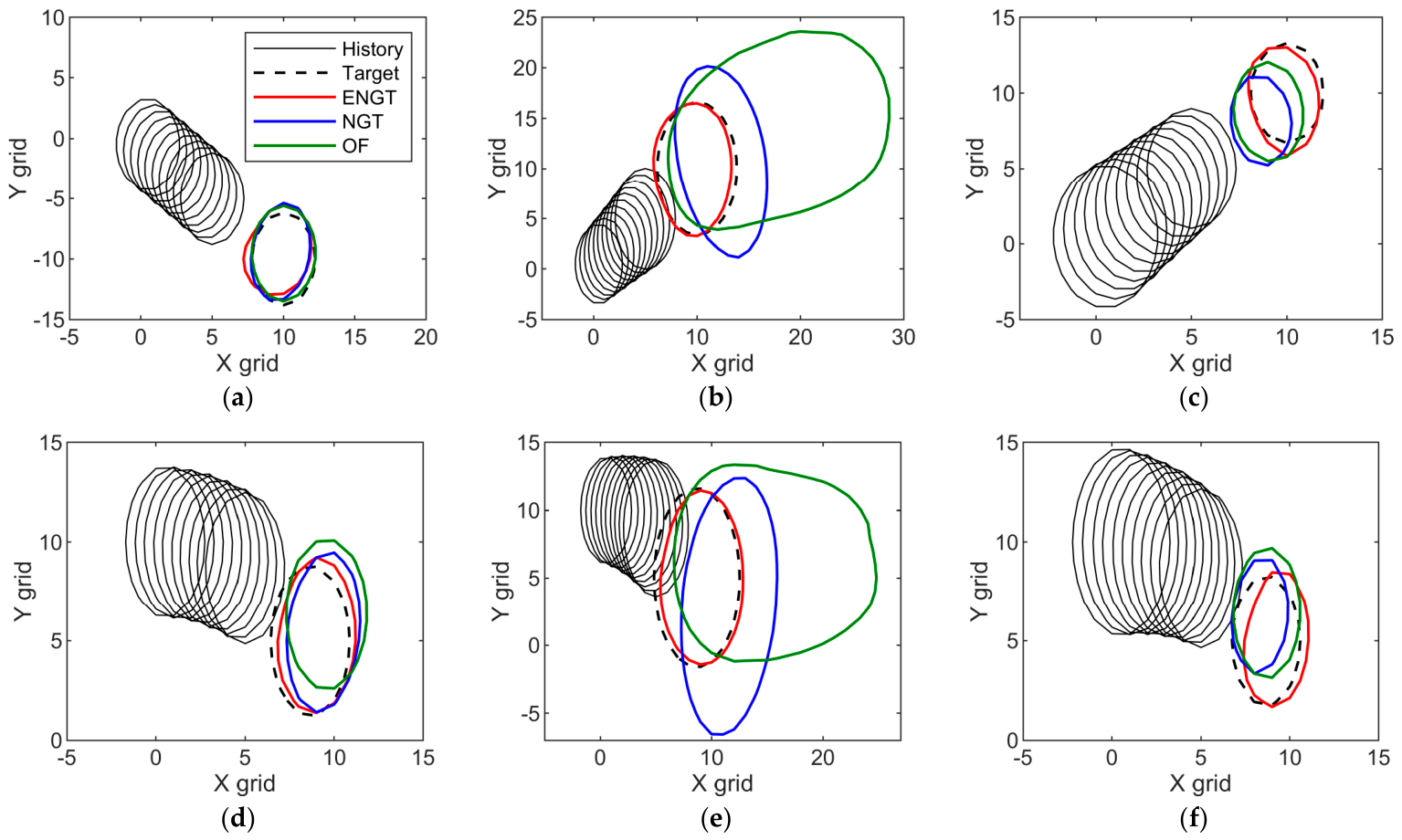
When only translation is present (Figure 3a), the results of the ENGT, NGT, and OF methods are almost identical and coincide with the expected prediction target. This can also be regarded as a basic verification for the three methods. The OF method results in larger errors when the radar echo increases and decreases (Figure 3b,e), mainly because these changes violate the assumption of constant brightness between consecutive time steps, which underlies OF estimation. When there is a turn in the path (Figure 3d–f), the OF method results also have obvious deviations because the algorithm itself does not reflect the mechanism of subsequent changes in the path. It is easy to imagine that even if more historical times are used to average the displacement vector field obtained by the OF scheme or if the OF scheme is used at a larger time and space scale, the center of the prediction result will be located only on the extension line of the target connection at certain times in the history, and it is impossible to predict that the target will continue to move clockwise, as shown in Figure 3d–f, resulting in greater deviation of the results. This is the reason why the OF-E1 and OF-E2 methods need not be shown here. The NGT method performs noticeably better than the OF scheme in more than half of the cases (Figure 3b,d,e), although the extrapolated field still differs from the target. In contrast, the ENGT method outperforms the other two methods in terms of changes in direction and evolution. Although complete overlap with the target is not achieved, the results demonstrate that the ENGT method fulfills the expectation of radar reflectivity changes and has an enhanced ability to predict radar echo movement.

3.1.2. The Impact of the Key Steps of ENGT

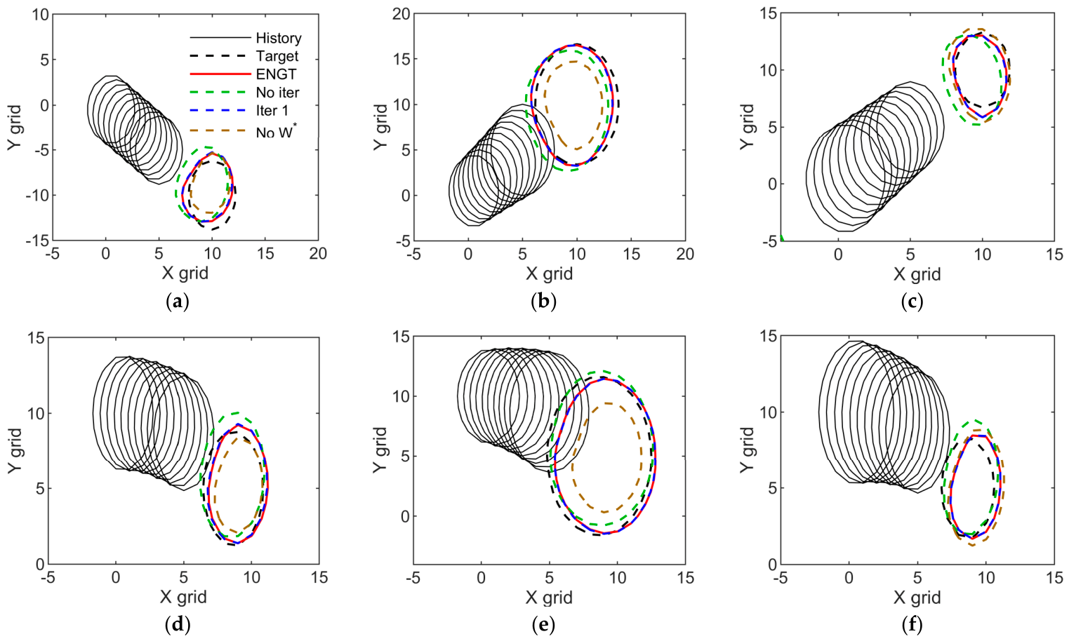
To reveal the impact of the main steps of the ENGT method, which are in addition to those of the NGT method, the same ideal experiments shown in Figure 3 are used, but key steps are controlled or removed for comparison (Figure 4). First, when M3×9 is not solved iteratively, as described in Section 2.2.2, the results clearly deviate from the experimental results with only linear translation (green dotted line in Figure 4a). This is also a key difficulty encountered in the development of the ENGT method because simply upgrading the transformation matrix from 2 × 6 to 3 × 9 by adding terms of image values cannot predict even the simplest translation. This also shows the necessity of an iterative solution for M3×9. When only one iteration is used, the ENGT method can achieve results close to the target. Notably, some subtle differences exist between using one iteration and completing the iteration, but it is difficult to distinguish them with the naked eye in the figure. When the calculation steps involving the transformation vector component W* are removed, the image value is underestimated not only in the incremental experimental group (Figure 4b,e) but also in the non-incremental experimental group (Figure 4a,d). These findings indicate that some of the moving features are mistakenly characterized as features with increased or decreased image values, indicating that the ENGT method does not strictly separate and reproduce these two kinds of features mathematically. However, compared with the other methods, the ENGT method performs better in experiments with movement, numerical changes, and path changes, as shown in Figure 3.
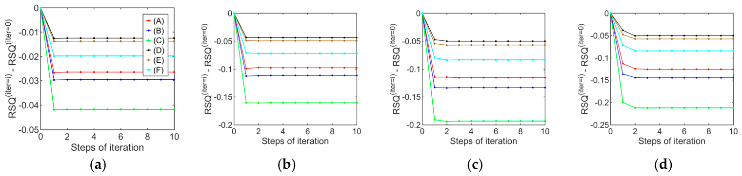
The variation in the residual sum of squares (RSQ) is used to show the influence of coefficient α and the iteration steps used to iteratively solve M3×9. The calculation steps are as follows:
C F ( i t e r = i )   =   B   M * ( i t e r = i )
RSQ = C F ( i t e r = i ) C ( i t e r = i ) 2
where the meanings of C, B, and M* are the same as those in Equations (12), (16) and (17). The superscript “iter = i” represents the ith iteration. CF(iter=i) is a vector with the same size as C(iter = i), which is derived from the existing B and solved M*(iter=i). If the solution of Equations (12) and (17) is regarded as a multiple linear regression, CF is equivalent to the fitting result used to approximate C; thus, the RSQ is defined as the sum of squares of the differences between the two vectors CF(iter=i) and C(iter=i). More importantly, as mentioned in Section 2.2.1, the minimization of the cost function in Equation (8) is equivalent to the solutions to the linear equations in Equations (12) and (17); that is, the RSQ here is equivalent to the value of the cost function to be minimized. Therefore, the convergence of the solution can be observed by the change in the RSQ.
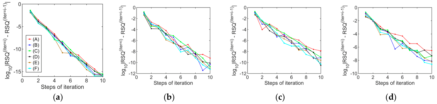
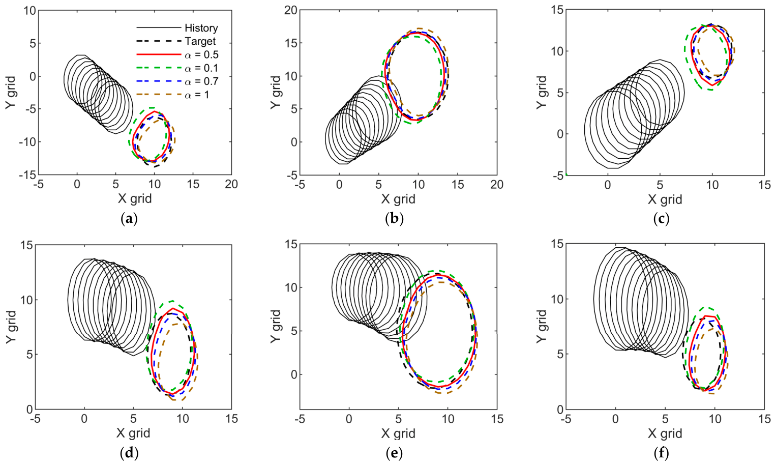
For the RSQ relative to non-iterative situations (Figure 5), on the one hand, different α values under the same ideal experiment produce different results, which indicates that the value of C may still not be solved accurately by iteration; on the other hand, all the experiments show that the RSQ tends to stabilize after no more than three iterations. The difference between adjacent iteration steps shows some oscillation (Figure 6), indicating that the convergence is not complete, and the amount shown in Figure 6 is taken in absolute value because the RSQ in some iteration steps is slightly increased. However, considering that Figure 6 is the result of log10, the overall convergence is obvious, indicating that empirical convergence is realized at least. Further comparison of different α values after 10 iterations (Figure 7) reveals that the underestimation of translation is the most obvious when α = 0.1, whereas the translation is overestimated when α = 1.0. Combined with Figure 6, it can be observed that the convergence speed of α = 0.5 is faster than that of α = 0.7, where the change in RSQ in all the experimental groups becomes less than 10−8 within 10 iterations. Therefore, α = 0.5 can be considered a feasible value. In general, the approach for solving M3×9 described in this study is not mathematically perfect; however, it can be used as a temporary scheme that provides a solution close to the goal.

3.2. Real Case 1: Cloud System with Convective Lines

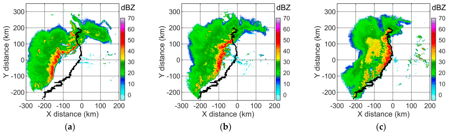
The selected forecast time and images from 1 h before and after are shown in Figure 8. As mentioned in Section 2.1, under the joint influence of the cells moving northeastward and new cells emerging on the right side, the convective line gradually moves eastward and evolves into a bow echo, with more cells in the southern part of the system. The enhanced echoes in the rear stratiform region are influenced mainly by the melting layer and the intensification of stratiform precipitation.
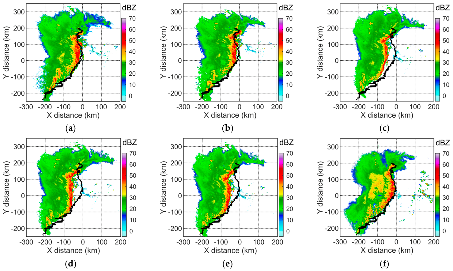
A comparison of different methods (Figure 9) reveals that both the ENGT and NGT methods properly extrapolated the position and bow shape of the convective line after 1 h, indicating that ENGT inherits the advantages of the NGT in this case and can stretch and distort the whole image along the overall moving direction of the cloud system (or the composite direction of cell movement and emergence) in this right-shift storm system to achieve prediction. The three OF methods seem to fail to correctly predict the position and overall shape of the convection line; they mainly extrapolate the echo northeastward along the direction of the mid- to low-level airflow [21]. As described in the ideal experiment in Section 3.1.1, the internal mechanism of the OF method makes it unable to reflect the situation in which the subsequent path is still changing. The OF method may be more suitable for frontal cyclone precipitation cloud systems with traceable large-scale circulation. On the other hand, the ENGT method generates more and stronger cells in the southern part of the cloud system, which aligns better with the observations. Additionally, although there are still differences in the radar reflectivity field compared with the observed stratiform cloud region, the reflectivity field at the rear of the storm in the ENGT method shows more intense precipitation compared with the other two methods, indicating that it reflects the reflectivity enhancement trend in the stratiform cloud region.
The skill score (Table 1) demonstrated that the ENGT method achieved higher CSI and POD values at 30 and 40 dBZ than those of all the other methods, but the magnitude of the lead over the NGT method was relatively small. In terms of the FSS and error statistics, the ENGT method is slightly lower or flatter than the NGT method. The scores of the three OF methods are high and low, but owing to the overall failure to properly predict the location of the cloud system, the scores are very close to the PB scheme. In general, the ENGT method is better than the PB and OF methods in this case. Although the improvement is limited compared with that of the NGT method, some of the higher scores prove that the ENGT method has the potential to predict reflectivity enhancement.

3.3. Real Case 2: Convective Cloud Cluster Developing from Weak Radar Echoes

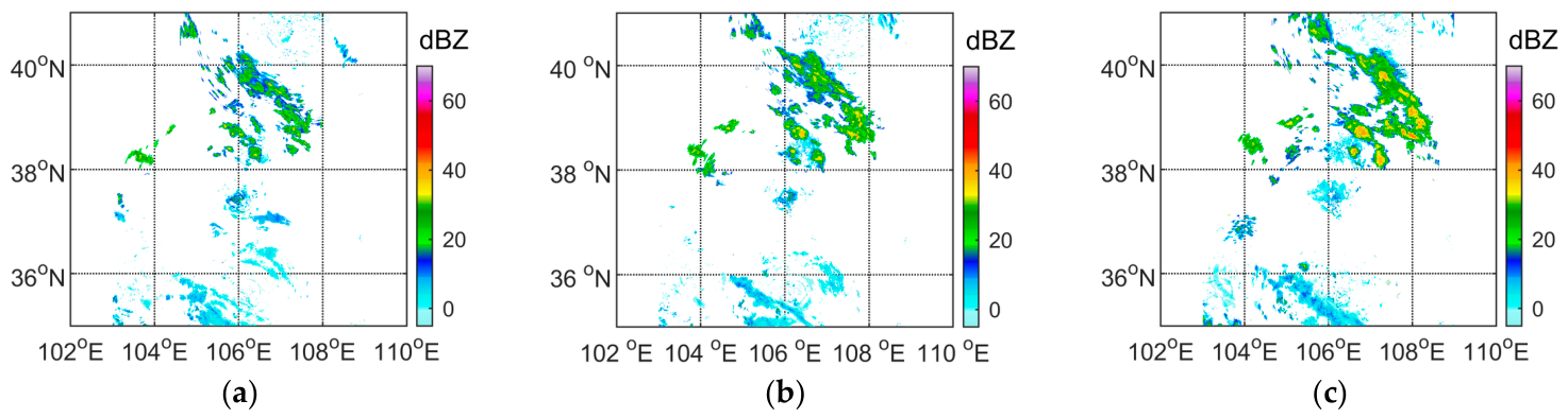
The convective cloud cluster moved eastward and developed from weak reflectivity (approximately 20 dBZ) to convective cloud precipitation with a maximum reflectivity exceeding 50 dBZ within 2 h (Figure 10). Starting from the time when the convective cores had reflectivities below 35 dBZ, the following section analyzes whether strong echoes consistent with the observations can be extrapolated 1 h later.
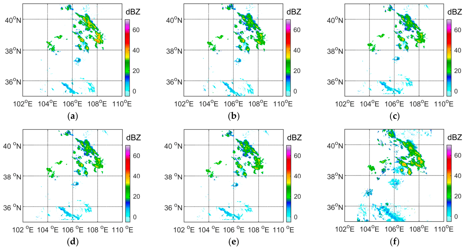
The 1 h extrapolation results (Figure 11) show that all the methods can predict the eastward movement of the cloud system, and the ENGT method can predict stronger cells with reflectivities exceeding 50 dBZ, as expected. Although scattered convective clouds lead to overall lower skill scores, the ENGT method still outperforms the other methods across almost all the statistical metrics (Table 2). Given that the FAR of the ENGT method at 40 dBZ is still high, the advantage of ENGT in this case is more likely attributable to its ability to generate strong reflectivity signals, which other methods fail to produce, rather than to a better positional forecast in this case.

3.4. Real Case 3: Isolated Hailstorm

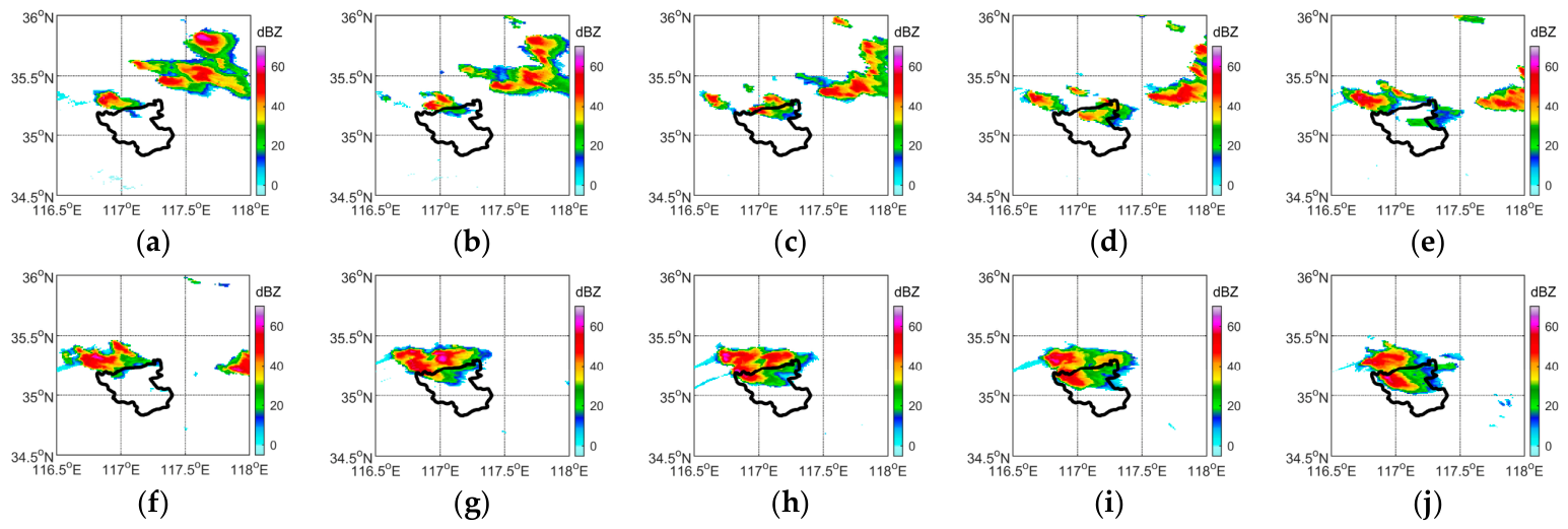
During the selected event, scattered strong convective clouds were active 100–300 km north of the Z9516 radar. The hail-producing cloud described below was located approximately 100 km north of the radar. Before 9:45, the cells moved mainly from west to east, and then one cell seemingly split from the cell on the northwest side of Tengzhou, moved southeastward, and gradually entered Tengzhou. The hailfall time was approximately 10:42 (the moment in Figure 12j). This can also be regarded as a kind of right-moving storm, where the low-level southerly inflow is more likely to strengthen or regenerate the cell along the southerly side.
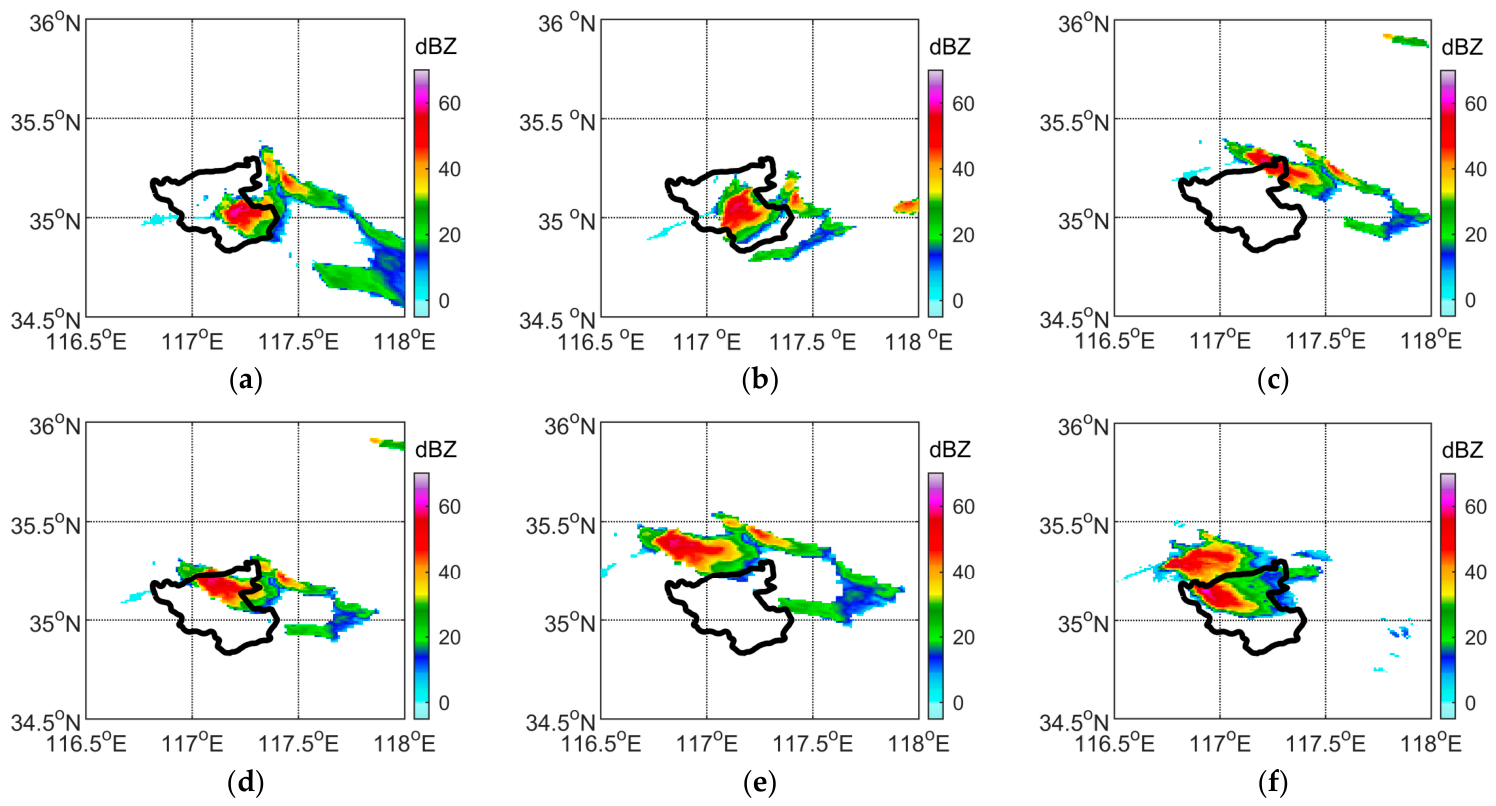
The results of the original experimental plan (Figure 13) show that the ENGT, NGT, and OF-E1 methods properly predicted the entry of the hail cloud into the Tengzhou boundary, but there seems to be an overestimation of movement. The OF method predicted that the cell directly moved eastward, whereas the OF-E2 method seemed to seriously underestimate cell movement. However, the skill score (Table 3) shows a rare and embarrassing problem; that is, the displacement and change in the original cloud body that splits the hail cloud are very limited, which leads to a high PB score, while the scores from the other methods are not as high as those of the PB scheme. The results of the OF-E2 method slightly exceed those of the PB method for some indicators; however, this is due to its underestimation of monomer movement, which makes it close to the results of the PB scheme; thus, it is difficult to say that the OF-E2 method produced better predictions. Furthermore, the multiple scores of the ENGT method at this time were worse than those of the other methods. This shows that predicting such a fast-developing and highly uncertain isolated cell storm is very challenging.
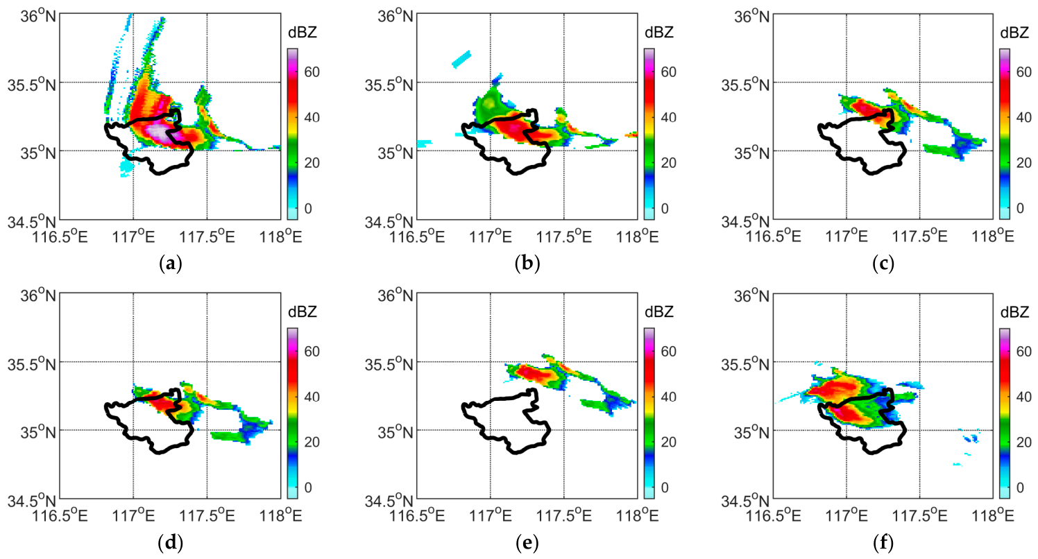
However, after further attempts were made, only data within an approximately 100 km radius around the hail-affected counties (200 km × 200 km range) were used as inputs for ENGT and the other methods, the PB scheme was excluded owing to the coincidence mentioned above, and the predicted reflectivity fields changed greatly (Figure 14). The results of the ENGT and NGT methods show a horizontal V shape similar to that of the target, whereas the predicted reflectivity of the ENGT method is stronger and hits stronger reflectivity grids. This leads to the ENGT method, with values of 30 and 40 dBZ, outperforming the other methods (Table 4), with the second-best method being NGT.
Notably, narrowing the range of input data is a retrospective selection because the location of hailfall cannot be determined in advance under real conditions. If trying to objectively select a smaller data space range by tracking some strong echoes, the original problem in strong convection warning still occurs; that is, the convective echoes may change rapidly and merge and split, which makes tracking difficult. Another approach is to consider the limited space where hail suppression operations are needed. For example, in real case 3, the NGT and ENGT methods achieve warning of convective cloud movement one hour in advance when a single 600 km × 600 km CAPPI radar is used as input. Then, the meteorological personnel in Tengzhou can continue to implement the ENGT method for a smaller area around Tengzhou, that is, focusing on the county with early warning needs; moreover, they can make decisions regarding issues such as artificial hail suppression through the prediction results of reflectivity enhancement or weakening.
In addition, inputs with a smaller area were not attempted, as early warnings with a radius of less than 100 km are less practical in terms of lead time (e.g., a wind speed of 20 m s−1 in the middle and lower layers can lead to a distance of 72 km in an hour).

3.5. Overall Statistics of 22 Precipitation Events

To facilitate the superposition of multiple events for overall statistics, the 3069 h result time is converted to hours relative to the time when the 45 dBZ echo area reaches the maximum in a current precipitation event, which is convenient for reflecting the characteristics of the results in the early, middle and late stages of the precipitation process. In view of the limited space, the simplest OF method is used as a representative of OF methods, and the focus is mainly on the CSI.
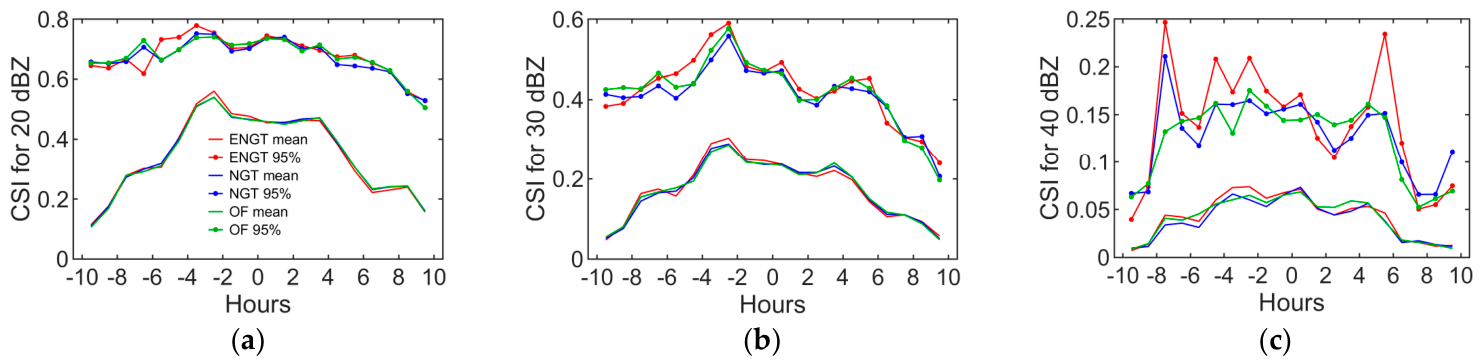
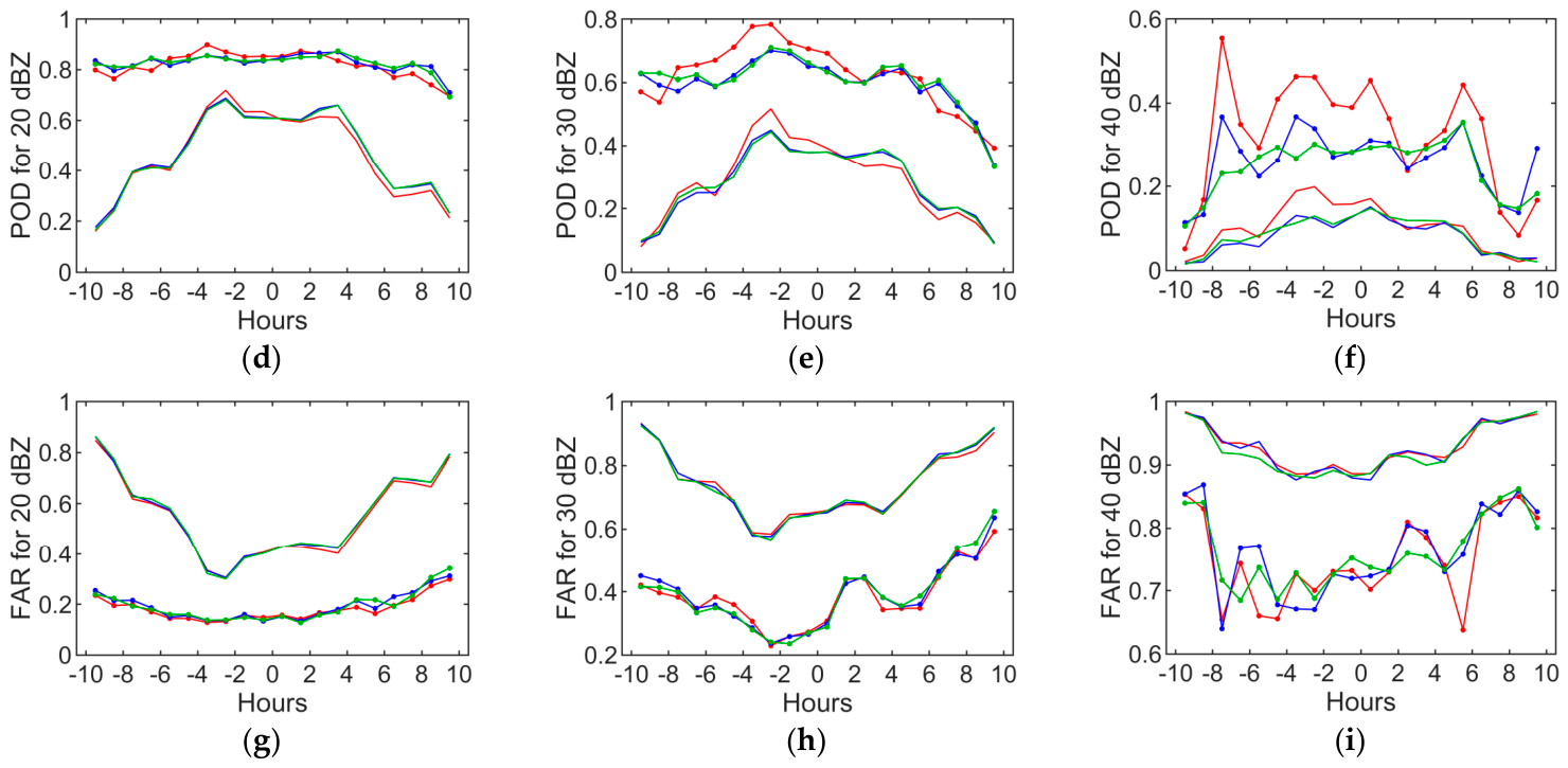
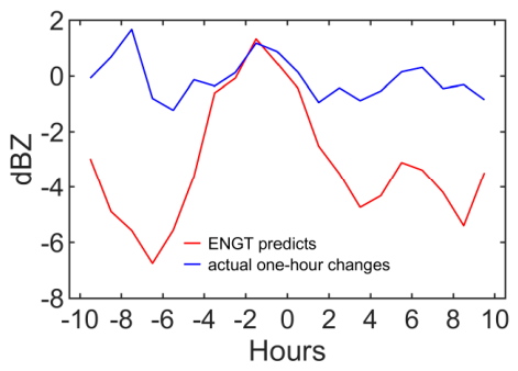
According to the average basic skill score (Figure 15), the curves of the different methods are very close. The CSI reaches relatively large values during the −4~4 h period. However, by observing the 95% quantile value, it can be found that the strong reflectivity prediction of ENGT in the early to middle period seems to be better. For example, the POD and CSI of ENGT at 30 and 40 dBZ are higher in the −5~0 h period, which indicates that ENGT leads to stronger reflectivity hits by generating stronger reflectivity. Other complementary comparisons (Figure 16) reveal that the ENGT’s strong reflectivity in the early- to mid-term is unlikely to be due to the abnormal increase mentioned in Section 3.4 because the maximum reflectivity predicted by ENGT in the −4~0 h period is very close to the actual one-hour changes. The comparison results of these average values at least reveal that a false alarm caused by abnormal amplification is not a very common phenomenon in ENGT. On the other hand, except for the above periods, ENGT underestimates the maximum reflectivity on average.
The quantitative CSI and significance statistics are given in Table 5. The T-test function of MATLAB 2020a was used to directly obtain the significance values of the CSI of ENGT with those of the other methods, thus eliminating the need to record the T value, confidence interval and lookup table according to the degree of freedom. The CSI derived from all the samples (total CSI in Table 5) revealed that ENGT was slightly greater than NGT, OF and PB. However, in terms of the average CSI, although significantly better than that of the PB method, which is a baseline, the CSI of ENGT is only slightly higher at 30 and 40 dBZ and significantly better than that of NGT at 40 dBZ but not significantly better than that of OF. Further significance tests for each hour in Figure 15 reveal that the CSI at 40 dBZ of ENGT is significantly better than that of NGT only in the −3~−2 h period and significantly better than that of OF in the −3~−4 h period (limited by the length, these statistical results are shown in the Supplementary Materials). This result shows that ENGT is not significantly better than the traditional method for the prediction of all 3069 h. However, ENGT has potential for warning of strong echoes in the early to middle stages of the precipitation process.

3.6. Computational Resources

Computing time and resource consumption are important for evaluating the practicality of an algorithm or an operational method. In particular, for weather warning, the time required to produce a product should be one order of magnitude less than the time required for radar volume scanning to provide timely warning information and leave room for fault tolerance of software and hardware.
Table 6 compares the calculation times of the three methods in different cases, and the recorded time consumption values are the stable medians in multiple tests. The computer used is a high-performance PC with an Intel U9-285K CPU (24 threads, maximum frequency > 5 GHz) and sufficient DDR5 memory. The statistical results in Table 5 indicate that the NGT and ENGT methods are obviously more time-consuming than the OF method, since they contain multiple linear regression calculations, which have higher time complexity. However, in the demonstrated cases, the time consumption is 100 s, which can be deemed to be completed quasi-instantaneously. In addition, the time consumption of the ENGT and NGT methods is not obviously different in real case 1 and real case 3, which may benefit from the built-in optimization of the computing software for array operations and multiple linear regression (for example, more threads are automatically used for larger-scale calculations). In the above tests, the number of CPU threads used was not limited, but the CPU allocated to this task was monitored to occupy 12%~26%, which may lead to the time consumption of the ENGT method in these tests not always being obviously higher than that of the NGT method.
Further evaluation of the time consumption of each calculation step of the ENGT method (Table 7) reveals that the most time-consuming step is the extrapolation step, which is based on bilinear interpolation and step-by-step calculation. On the other hand, the time consumption of the steps, such as listing the B and C coefficients, solving M3×9, and iteration, is very small, indicating that the additional calculation content of the ENGT method compared with the NGT method is not enough to lead to a doubling of the calculation time.
In terms of memory usage, owing to the cache mechanism of the computing software, the increase in memory at runtime fluctuates during repeated runs, and detailed statistical results are not listed here. However, according to the statistics, the memory occupied by the ENGT algorithm does not exceed 2 GB, and the percentage increase in memory usage compared to the OF and NGT methods fluctuates between 10% and 100%. In general, this is still within the range that general contemporary computers can handle.
The above tests do not include reading radar raw data, preprocessing, or degradation. In these tests, the time consumption for the degradation of 10~14 600 × 600 images is generally less than 0.5 s according to the method described in Section 2.2.4. For reading radar data and calculating the composite reflectivity or CAPPI, the main time consumption may be decompression and interpolation operations. Under an appropriate interpolation method (such as the trilinear interpolation method mentioned above), the time consumption of processing the volume scan data of a typical traditional mechanical scanning radar can be controlled within 10 s, while the time consumption of processing the volume scan data of the phased array radar with more elevation angles and distance gates can be controlled within 30 s. Therefore, the ENGT method is sufficient to provide timely products for a traditional mechanical scanning radar that observes volume scan data every 4~6 min; for a phased array radar volume scan data acquired every 30 s~1 min, the ENGT method also has potential for application with quasi-instantaneous operation time.

4. Discussion

4.1. Advantages of the ENGT Method

The results of a set of ideal experiments and three real experiments reveal that the ENGT method essentially achieves the development goal of simultaneously predicting echo movement, shape changes, and intensity changes.
In the demonstrated ideal experiments, owing to the inclusion of nonlinear terms related to image values in the transformation matrix and the further iterative solution method described in this study, the ENGT method was able to achieve results that were visually very close to expectations. This represents a significant improvement over the original NGT method, which was only partially or slightly better than the traditional OF method.
In the demonstrated real experiments, which included squall lines and convective cell clusters, compared with the other two types of methods, the more accurate predictions of echo intensity or position by the ENGT method resulted in higher skill scores. These results at least preliminarily indicate that the 3 × 9 nonlinear transformation matrix proposed in this study can reflect and predict the complex combined changes in the echo displacement, deformation, and intensity of convective cloud systems. Moreover, the computational efficiency of the ENGT method is not obviously lower than that of the OF and NGT methods within the detection range of a single weather radar, which provides the basis for the practical application of the ENGT method.

4.2. Other Known Issues and Limitations

Although the ENGT method demonstrated promising results in this study, several issues and limitations remain and are discussed below.
(1) Similar to the NGT method, the ENGT method exhibits edge effects, meaning that the extrapolated edges of convective cells may exhibit shape distortions, as shown in Figure 1. Particularly, when the echo area is very small, this edge effect may start from the periphery of the echo, potentially causing parts of the echo image to appear stretched into unusual shapes, similar to the northern region in Figure 14a.
(2) Statistical tests of more than 3000 h of predicted results reveal that ENGT does not yet have a strict statistical advantage. Owing to the limited sample size, the cause of these results has not been determined. The data quality of the radar mosaic and the size of the spatial range of the input data are problems that still need to be solved; thus, the ENGT method currently has no definite absolute advantage over the other methods. However, when more samples are obtained in the future, the conditions under which the ENGT method is more likely to be better than other methods should be studied first.
(3) The methods discussed in this study still cannot predict convective initiation over an entirely clear sky. However, this is also a challenge faced by other extrapolation and prediction methods and even numerical weather forecasting.

5. Conclusions and Summary

Building upon the previously proposed NGT method, this study introduces the ENGT method, which is capable of extrapolating and predicting radar reflectivity fields. By treating the radar reflectivity as the third coordinate alongside the grid coordinates X and Y, the nonlinear transformation matrix is expanded, a solution method is derived, and the effectiveness is compared with that of the NGT and traditional OF methods in extrapolation experiments.
The results from a set of ideal experiments demonstrated better performance of the ENGT method in predicting the numerical change and path change in images that contain simple targets. The ENGT method also shows potential in selected typical real cases. In a prediction experiment for squall line clouds, the ENGT method predicted the overall movement direction of the cloud system synthesized by moving and emerging cells, a capability inherited from the NGT method, and obtained higher skill scores because it predicted stronger reflectivity. In an enhancing convective cloud cluster prediction experiment, the ENGT method also achieved higher scores because it generated stronger reflectivity. In a retrospective prediction experiment of an isolated hailstorm, a small range of input data enabled the ENGT method to predict stronger reflectivity grids. In addition, the computational efficiency for a single weather radar was considerable.
This study also reveals many limitations of the ENGT method. First, the ENGT method is not perfect in terms of mathematical solutions. The lack of a convergence proof, the abnormal stretching of image edges, and the nonlinear amplification of reflectivity are all potential problems, indicating that the algorithm still needs to be improved. Thus, the ENGT method has not yet achieved a statistically significant advantage given the limited number of samples. Therefore, the ENGT method cannot completely replace the original NGT and traditional OF methods at this stage. Furthermore, the optimal spatial scale and weather type of the ENGT method have not yet been determined, which may explain why the skill score of ENGT is not yet significantly higher than that of the traditional method. However, with the accumulation of more samples and prediction cases in the future, the conditions under which the ENGT method is more likely to outperform other methods should be studied.

Supplementary Materials

The following supporting information can be downloaded at https://www.mdpi.com/article/10.3390/rs18172865/s1, Figure S1: Screenshot of the plot result of ideal experiment b using the above plotting codes; Figure S2: The experiment of changing the input grid resolution; Figure S3: The experiment of changing the standard deviation of two-dimensional Gaussian filtering; Figure S4: The experiment of changing the radius of 10 grids of the two-dimensional Gaussian filtering; Table S1: The CSI for 20 dBZ of 1 h extrapolation using different methods in 22 precipitation events and significance; Table S2: The CSI for 30 dBZ of 1 h extrapolation using different methods in 22 precipitation events and significance; Table S3: The CSI for 40 dBZ of 1 h extrapolation using different methods in 22 precipitation events and significance.

Author Contributions

Conceptualization, T.Y. and Y.S.; methodology, H.Y. and Y.S.; software, S.L.; validation, T.Y., S.L., and Z.L.; formal analysis, T.Y.; investigation, Y.S.; resources, S.L. and Z.L.; data curation, S.L. and Z.L.; writing—original draft preparation, T.Y. and Y.S.; writing—review and editing, H.Y. and Z.L.; visualization, T.Y. and S.L.; supervision, H.Y. and Y.S.; project administration, H.Y. and Y.S.; funding acquisition, H.Y. and Y.S. All authors have read and agreed to the published version of the manuscript.

Funding

This research was funded by the Strategic Priority Research Program of the Chinese Academy of Sciences (Grant No. XDB0760402), the Civil Aircraft Special Research Project (Grant No. MJZ5-1N22), the National Natural Science Foundation of China (Grant No. 42475160), the Science and Technology Program of Guizhou Province (Grant No. Qiankehe Zhicheng [2023] General 193), and the Fundamental Research Funds of the Institute of Atmospheric Physics, Chinese Academy of Sciences.

Data Availability Statement

Data are available in a publicly accessible repository that does not issue DOIs. Publicly available datasets were analyzed in this study. The data used in Section 3.1 can be found in Appendix A. The raw data of the NEXRAD radar base data used in Section 3.2 can be found at https://www.ncdc.noaa.gov/nexradinv/map.jsp (accessed on 20 August 2026), where they have been accessible since 7 February 2023. Other data presented in this study are available on request from the corresponding author due to data sharing policies and sharing forms in different demonstrated cases.

Conflicts of Interest

The authors declare no conflicts of interest.

Appendix A

The basic form of the input sample at a specific time for the ideal experiments in Section 3.1 is as follows (Equation (A1)):
Q(x,y) = A·exp(−((xxc)2/qstd + (y - yc)2/3/qstd)) + ΔQ
where all the variables can be considered dimensionless. Q is the value of a two-dimensional image along the x and y dimensions. x and y range from −40 to 40, with a spacing of 1. The right side of the equal sign generally represents a two-dimensional normal distribution. xc and yc are the center locations of the normal distribution, which vary with time and are used to represent changes in a target in images. ΔQ represents the increase or decrease in the image value with time. A is a constant that determines the overall amplitude of the image. qstd is a parameter that controls the shape of the distribution, which is similar to the standard deviation in a normal distribution. The values of xc, yc, A, and ΔQ are calculated on the basis of time t, and they are defined in different experimental groups as follows:
(a) Translation only
A = 1, xc = 0.5t, yc = −0.5t, ΔQ = 0
(b) Translation + growth
A = 1, xc = 0.5t, yc = 0.5t, ΔQ = 0.01t
(c) translation + decay
A = 1.2, xc = 0.5t, yc = 0.5t, ΔQ = −0.008t
(d) Direction change
A = 1, xc = 10·sind(3t), yc = 10·cosd(3t), and ΔQ = 0, where “sind” and “cosd” are the trigonometric functions sine and cosine, respectively, with the degree values as the input. The same is true below.
(e) Direction change + growth
A = 1, xc = 10·sind(3t), yc = 10·cosd(3t), ΔQ = 0.01t
(f) Direction change + decay
A = 1.2, xc = 10·sind(3t), yc = 10·cosd(3t), ΔQ = −0.008t

References

  1. Chen, S.; Shu, T.; Zhao, H.; Zhong, G.; Chen, X. TempEE: Temporal–spatial parallel transformer for radar echo extrapolation beyond autoregression. IEEE Trans. Geosci. Remote Sens. 2023, 61, 1–14. [Google Scholar] [CrossRef] [Scilit]
  2. Li, P.W.; Lai, E.S.T. Applications of radar-based nowcasting techniques for mesoscale weather forecasting in Hong Kong. Meteorol. Appl. 2004, 11, 253–264. [Google Scholar] [CrossRef] [Scilit]
  3. Liang, Q.; Feng, Y.; Deng, W.; Hu, S.; Huang, Y.; Zeng, Q.; Chen, Z. A composite approach of radar echo extrapolation based on TREC vectors in combination with model-predicted winds. Adv. Atmos. Sci. 2010, 27, 1119–1130. [Google Scholar] [CrossRef] [Scilit]
  4. Zou, H.; Wu, S.; Shan, J.; Yi, X. A method of radar echo extrapolation based on TREC and Barnes filter. J. Atmos. Ocean. Technol. 2019, 36, 1713–1727. [Google Scholar] [CrossRef] [Scilit]
  5. Woo, W.C.; Wong, W.K. Operational application of optical flow techniques to radar-based rainfall nowcasting. Atmosphere 2017, 8, 48. [Google Scholar] [CrossRef] [Scilit]
  6. Ayzel, G.; Heistermann, M.; Winterrath, T. Optical flow models as an open benchmark for radar-based precipitation nowcasting (rainymotion v0.1). Geosci. Model Dev. 2019, 12, 1387–1402. [Google Scholar] [CrossRef] [Scilit]
  7. Long, Y.; Kang, X.; Zhang, L.; Li, F. Research on the application of weather radar echo extrapolation technology in nowcasting of civil aviation meteorology. Adv. Meteorol. 2025, 2025, 5569646. [Google Scholar] [CrossRef] [Scilit]
  8. Dixon, M.; Wiener, G. TITAN: Thunderstorm identification, tracking, analysis, and nowcasting—A radar-based methodology. J. Atmos. Ocean. Technol. 1993, 10, 785–797. [Google Scholar] [CrossRef] [Scilit]
  9. Crane, R.K. Automatic radar cell detection and tracking. Bull. Am. Meteorol. Soc. 1979, 60, 568–569. [Google Scholar]
  10. Johnson, J.T.; MacKeen, P.L.; Witt, A.; Mitchell, E.D.; Stumpf, G.J.; Eilts, M.D.; Thomas, K.W. The storm cell identification and tracking algorithm: An enhanced WSR-88D algorithm. Weather Forecast. 1998, 13, 263–276. [Google Scholar] [CrossRef] [Scilit]
  11. Pan, X.; Lu, Y.; Zhao, K.; Huang, H.; Wang, M.; Chen, H. Improving nowcasting of convective development by incorporating polarimetric radar variables into a deep-learning model. Geophys. Res. Lett. 2021, 48, e2021GL095302. [Google Scholar] [CrossRef] [Scilit]
  12. Yao, J.; Xu, F.; Qian, Z.; Cai, Z. A forecast-refinement neural network based on DyConvGRU and U-Net for radar echo extrapolation. IEEE Access 2023, 11, 53249–53261. [Google Scholar] [CrossRef] [Scilit]
  13. Shi, X.; Chen, Z.; Wang, H.; Yeung, D.-Y.; Wong, W.-K.; Woo, W.-C. Convolutional LSTM network: A machine learning approach for precipitation nowcasting. In Advances in Neural Information Processing Systems; Curran Associates, Inc.: Red Hook, NY, USA, 2015; Volume 28, pp. 802–810. [Google Scholar]
  14. Shi, X.; Gao, Z.; Lausen, L.; Wang, H.; Yeung, D.-Y.; Wong, W.-K.; Woo, W.-C. Deep learning for precipitation nowcasting: A benchmark and a new model. In Advances in Neural Information Processing Systems; Curran Associates, Inc.: Red Hook, NY, USA, 2017; Volume 30, pp. 5617–5627. [Google Scholar]
  15. Wang, Y.; Long, M.; Wang, J.; Gao, Z.; Yu, P.S. PredRNN: Recurrent neural networks for predictive learning using spatiotemporal LSTMs. In Advances in Neural Information Processing Systems; Curran Associates, Inc.: Red Hook, NY, USA, 2017; Volume 30. [Google Scholar]
  16. Zhang, Y.; Long, M.; Chen, K.; Xing, L.; Jin, R.; Jordan, M.I.; Wang, J. Skilful nowcasting of extreme precipitation with NowcastNet. Nature 2023, 619, 526–532. [Google Scholar] [CrossRef] [Scilit] [PubMed]
  17. Wu, W.; He, G.; Zhuang, X.; Feng, Y.; Sun, J.; Chen, H.; Lei, L.; Luo, J. Global-frequency synergy: A novel paradigm for radar echo extrapolation via attention and Fourier convolution. J. Geophys. Res. Atmos. 2026, 131, e2025JD045579. [Google Scholar] [CrossRef] [Scilit]
  18. Geng, H.; Wu, F.; Zhuang, X.; Geng, L.; Xie, B.; Shi, Z. MS-RadarFormer: A transformer-based multiscale deep learning model for radar echo extrapolation. Remote Sens. 2024, 16, 274. [Google Scholar] [CrossRef] [Scilit]
  19. Ravuri, S.; Lenc, K.; Willson, M.; Kangin, D.; Lam, R.; Mirowski, P.; Fitzsimons, M.; Athanassiadou, M.; Kashem, S.; Madge, S.; et al. Skilful precipitation nowcasting using deep generative models of radar. Nature 2021, 597, 672–677. [Google Scholar] [CrossRef] [Scilit] [PubMed]
  20. Wu, Q.; Wang, X.; Zhang, T.; Miao, Z.; Ye, W.; Li, H. DiffREE: Feature-conditioned diffusion model for radar echo extrapolation. J. Supercomput. 2025, 81, 30. [Google Scholar] [CrossRef] [Scilit]
  21. Sun, Y.; Xiao, H.; Tian, Y.; Yang, H. A nonlinear grid transformation method for extrapolating and predicting the convective echo of weather radar. Remote Sens. 2023, 15, 1406. [Google Scholar] [CrossRef] [Scilit]
  22. Xue, L.; Fan, J.; Lebo, Z.J.; Wu, W.; Morrison, H.; Grabowski, W.W.; Chu, X.; Geresdi, I.; North, K.; Stenz, R.; et al. Idealized simulations of a squall line from the MC3E field campaign applying three bin microphysics schemes: Dynamic and thermodynamic structure. Mon. Weather Rev. 2017, 145, 4789–4812. [Google Scholar] [CrossRef] [Scilit]
  23. Ren, G.; Sun, Y.; Sun, H.; Dong, Y.; Yang, Y.; Xiao, H. A Case Study on Two Differential Reflectivity Columns in a Convective Cell: Phased-Array Radar Observation and Cloud Model Simulation. Remote Sens. 2024, 16, 460. [Google Scholar] [CrossRef] [Scilit]
  24. Sun, Y.; Xiao, H.; Yang, H.; Chen, H.; Feng, L.; Shu, W.; Yao, H. A Uniformity Index for Precipitation Particle Axis Ratios Derived from Radar Polarimetric Parameters for the Identification and Analysis of Raindrop Areas. Remote Sens. 2023, 15, 534. [Google Scholar] [CrossRef] [Scilit]
  25. Ayzel, G.; Scheffer, T.; Heistermann, M. RainNet v1.0: A convolutional neural network for radar-based precipitation nowcasting. Geosci. Model Dev. 2020, 13, 2631–2644. [Google Scholar] [CrossRef] [Scilit]
  26. Pulkkinen, S.; Nerini, D.; Pérez Hortal, A.A.; Velasco-Forero, C.; Seed, A.; Germann, U.; Foresti, L. Pysteps: An open-source Python library for probabilistic precipitation nowcasting (v1.0). Geosci. Model Dev. 2019, 12, 4185–4219. [Google Scholar] [CrossRef] [Scilit]
  27. Seed, A.W. A dynamic and spatial scaling approach to advection forecasting. J. Appl. Meteorol. 2003, 42, 381–388. [Google Scholar] [CrossRef] [Scilit] [PubMed]
  28. Roberts, N.M.; Lean, H.W. Scale-selective verification of rainfall accumulations from high-resolution forecasts of convective events. Mon. Weather Rev. 2008, 136, 78–97. [Google Scholar] [CrossRef] [Scilit]
  29. Antonio, B.; Aitchison, L. How to derive skill from the Fractions Skill Score. Mon. Weather Rev. 2025, 153, 1021–1033. [Google Scholar] [CrossRef] [Scilit]
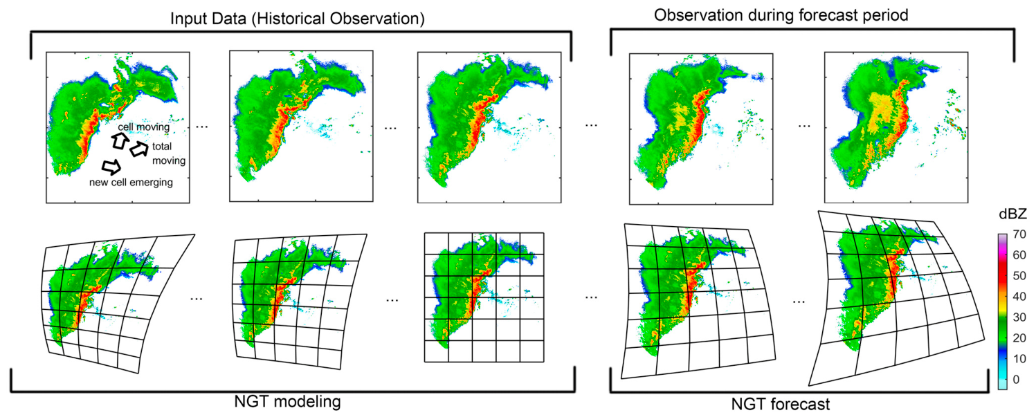
Figure 1. Conceptual diagram of the NGT method.
Remotesensing 18 02865 g001
Figure 2. Conceptual diagram of the ENGT method.
Remotesensing 18 02865 g002
Figure 3. Ideal predictions using the ENGT, NGT, and OF methods under typical scenarios. (a) Translation only; (b) translation + growth; (c) translation + decay; (d) direction change; (e) direction change + growth; and (f) direction change + decay. The specific settings of the input and target samples can be found in Appendix A. The circles are contours with a value of 0.5. The black solid circles represent the 10 historical time steps used as the input for parameter estimation. The black dashed circles represent the 20th time step, i.e., the target. The colored circles show the results of each method when the 10 time steps are extrapolated starting from the 10th time step.
Remotesensing 18 02865 g003
Figure 4. Similar to Figure 3 but for ideal predictions using the ENGT method and schemes that do not contain a key step of ENGT. (a) Translation only; (b) translation + growth; (c) translation + decay; (d) direction change; (e) direction change + growth; and (f) direction change + decay. The “No iter” scheme excludes iterative solving of M3×9. The “Iter 1” scheme contains only one iteration in the iterative solution of M3×9. The “No W*” scheme excludes calculation steps involving the transformation vector component W*.
Remotesensing 18 02865 g004
Figure 5. The variation in the residual sum of squares (RSQ) after Equation (12) is solved with different iteration steps and α values used in the ENGT method. (a) α = 0.1; (b) α = 0.5; (c) α = 0.7; and (d) α = 1.0. The values on the y-axis are RSQ(iter=i) − RSQ(iter=0), which is the difference between the RSQ in an iteration step (iter = i) and that without iteration (iter = 0). The (A)~(F) in the legend represent ideal experiments (a)~(f) that are the same as those in Figure 4.
Remotesensing 18 02865 g005
Figure 6. Similar to Figure 5 but for the absolute difference between the latter and the one from the adjacent previous iteration. (a) α = 0.1; (b) α = 0.5; (c) α = 0.7; and (d) α = 1.0. The values on the y-axis are log10|RSQ(iter=i) − RSQ(iter=i−1)|, which is the difference between the RSQ in an iteration step (iter = i) and the previous step (iter = I − 1). The (A)~(F) in the legend represent ideal experiments (a)~(f) that are the same as those in Figure 4.
Remotesensing 18 02865 g006
Figure 7. Ideal predictions using the ENGT method with different α values. (a) Translation only; (b) translation + growth; (c) translation + decay; (d) direction change; (e) direction change + growth; and (f) direction change + decay.
Remotesensing 18 02865 g007
Figure 8. CAPPI at 3 km height observed by the KTLX radar: (a) 1 h before the start of extrapolation; (b) at the start of extrapolation; and (c) 1 h after the start of extrapolation, i.e., the target time. The target time is 20 May 2011, 10:05 UTC. The black solid line represents the observed 30 dBZ reflectivity front at the target time.
Remotesensing 18 02865 g008
Figure 9. Comparison of 1 h extrapolation results for the KTLX radar CAPPI at 3 km altitude using different methods. (a) ENGT; (b) NGT; (c) OF; (d) OF-E1; (e) OF-E2; and (f) the target. Target time: 20 May 2011, 10:05 UTC. The black solid line represents the observed 30 dBZ reflectivity front at the target time.
Remotesensing 18 02865 g009
Figure 10. Composite reflectivity of the radar mosaic in northern Ningxia, China: (a) 1 h before the start of extrapolation; (b) at the start of extrapolation; and (c) 1 h after the start of extrapolation, i.e., the target time. The target time is 01:54 UTC on 11 July 2023.
Remotesensing 18 02865 g010
Figure 11. Comparison of the 1 h extrapolation results for the composite reflectivity from the radar mosaic in northern Ningxia obtained by different methods. (a) ENGT; (b) NGT; (c) OF; (d) OF-E1; (e) OF-E2; and (f) the target. The target time is 11 July 2023, 01:54 UTC.
Remotesensing 18 02865 g011
Figure 12. CAPPI at 3 km altitude observed by the Z9516 radar on 9 July 2023. (a) 08:48; (b) 09:00; (c) 09:11; (d) 09:22; (e) 09:45; (f) 09:56; (g) 10:08; (h) 10:19; (i) 10:30; and (j) 10:42. The time is UTC. (e) The start of extrapolation; (j) approximately 1 h after the start of extrapolation, i.e., the target time. The black solid line indicates the county where hail occurred at the target time: Tengzhou County, Shandong Province, China.
Remotesensing 18 02865 g012
Figure 13. Comparison of the 1 h extrapolation results for the 3 km height CAPPI from the Z9516 radar using different methods and 600 km × 600 km CAPPI as inputs. (a) ENGT; (b) NGT; (c) OF; (d) OF-E1; (e) OF-E2; and (f) the target. The black solid line indicates the county where hail occurred at the target time: Tengzhou, Shandong Province, China. The target time is 10:42 UTC on 9 July 2023.
Remotesensing 18 02865 g013
Figure 14. Comparison of 1 h extrapolation results for the 3 km height CAPPI from the Z9516 radar using different methods and 200 km × 200 km CAPPI as inputs. (a) ENGT; (b) NGT; (c) OF; (d) OF-E1; (e) OF-E2; and (f) the target. The black solid line indicates the county where hail occurred at the target time: Tengzhou, Shandong Province, China. The target time is 10:42 UTC on 9 July 2023.
Remotesensing 18 02865 g014
Figure 15. Averaged skill scores of 3069 h from 22 precipitation events in different stages: (a) CSI for 20 dBZ; (b) CSI for 30 dBZ; (c) CSI for 40 dBZ; (d) POD for 20 dBZ; (e) POD for 30 dBZ; (f) POD for 40 dBZ; (g) FAR for 20 dBZ; (h) FAR for 30 dBZ; and (i) FAR for 40 dBZ. The X-axis represents the time relative to the time at which the 45 dBZ echo area reaches a maximum during a precipitation event. The “95%” in the legend represents the 95% percentile value.
Remotesensing 18 02865 g015aRemotesensing 18 02865 g015b
Figure 16. Differences in maximum reflectivity. Red line: the maximum reflectivity of 1 h extrapolated by ENGT minus the maximum reflectivity at the start time of the extrapolation; blue line: the maximum reflectivity at the target time minus that at the start time. The X-axis represents the time relative to the time at which the 45 dBZ echo area reached a maximum in a precipitation event, and the points on the lines are the average values in each one-hour statistical period.
Remotesensing 18 02865 g016
Table 1. Skill scores and errors for 1 h extrapolation using different methods for real case 1. The darker gray and lighter gray areas indicate the best and second-best values, respectively.
StatisticPBOFOF-E1OF-E2NGTENGT
CSI for 20 dBZ0.530.600.470.430.680.68
CSI for 30 dBZ0.240.230.230.200.330.37
CSI for 40 dBZ0.040.040.060.050.250.28
POD for 20 dBZ0.700.750.690.640.840.83
POD for 30 dBZ0.310.290.300.260.410.48
POD for 40 dBZ0.070.080.130.110.420.49
FAR for 20 dBZ0.310.260.410.430.230.21
FAR for 30 dBZ0.490.440.470.520.380.37
FAR for 40 dBZ0.930.900.900.910.610.60
FSS(2) for 20 dBZ0.780.830.710.680.890.87
FSS(2) for 30 dBZ0.510.520.530.480.650.65
FSS(2) for 40 dBZ0.110.170.220.210.620.61
FSS(5) for 20 dBZ0.810.860.740.700.910.90
FSS(5) for 30 dBZ0.570.580.600.550.690.72
FSS(5) for 40 dBZ0.130.240.270.270.710.71
MAE (dBZ)2.261.942.662.811.531.66
RMSE (dBZ)7.086.417.467.855.045.26
CC0.720.770.690.660.860.85
MBias (dBZ)−0.12−0.420.06−0.03−0.090.09
Table 2. Skill scores and errors for 1 h extrapolation using different methods for real case 2. The darker gray and lighter gray areas indicate the best and second-best values, respectively.
StatisticPBOFOF-E1OF-E2NGTENGT
CSI for 20 dBZ0.120.280.300.180.320.40
CSI for 30 dBZ0.020.130.150.050.120.27
CSI for 40 dBZ0.000.000.000.000.000.03
POD for 20 dBZ0.190.360.390.260.420.51
POD for 30 dBZ0.040.160.190.070.160.43
POD for 40 dBZ0.000.000.000.000.000.09
FAR for 20 dBZ0.730.470.430.640.440.36
FAR for 30 dBZ0.930.640.570.850.680.58
FAR for 40 dBZ1.001.000.921.001.000.95
FSS(2) for 20 dBZ0.270.540.570.380.600.69
FSS(2) for 30 dBZ0.070.340.400.150.320.56
FSS(2) for 40 dBZ0.010.010.050.000.000.15
FSS(5) for 20 dBZ0.320.620.660.450.680.77
FSS(5) for 30 dBZ0.100.450.520.200.440.66
FSS(5) for 40 dBZ0.010.040.100.000.010.32
MAE (dBZ)2.852.061.982.451.981.84
RMSE (dBZ)7.766.185.977.055.985.66
CC0.240.520.560.380.570.63
MBias (dBZ)−0.60−0.76−0.77−0.69−0.61−0.58
Table 3. Skill scores and errors of 1 h extrapolation using different methods for real case 3, with 600 km × 600 km CAPPI input. The darker gray and lighter gray areas indicate the best and second-best values, respectively.
StatisticPBOFOF-E1OF-E2NGTENGT
CSI for 20 dBZ0.250.050.170.200.100.04
CSI for 30 dBZ0.230.010.050.220.040.01
CSI for 40 dBZ0.140.000.000.170.010.00
POD for 20 dBZ0.410.080.260.350.150.07
POD for 30 dBZ0.380.010.080.330.070.02
POD for 40 dBZ0.230.000.000.240.020.00
FAR for 20 dBZ0.610.880.660.670.790.92
FAR for 30 dBZ0.640.980.870.600.890.97
FAR for 40 dBZ0.741.001.000.650.971.00
FSS(2) for 20 dBZ0.480.120.360.410.220.09
FSS(2) for 30 dBZ0.440.020.140.440.110.03
FSS(2) for 40 dBZ0.310.000.020.370.030.00
FSS(5) for 20 dBZ0.540.140.440.480.250.10
FSS(5) for 30 dBZ0.510.030.220.520.140.04
FSS(5) for 40 dBZ0.380.000.110.470.060.00
MAE (dBZ)2.973.503.023.363.454.27
RMSE (dBZ)9.7910.899.9410.0810.8511.69
CC0.420.120.290.350.150.04
MBias (dBZ)−0.01−0.88−0.750.00−0.84−0.26
Table 4. Skill scores and errors of 1 h extrapolation using different methods for real case 3, with 200 km × 200 km CAPPI input and excluding the PB scheme. The darker gray and lighter gray areas indicate the best and second-best values, respectively.
StatisticOFOF-E1OF-E2NGTENGT
CSI for 20 dBZ0.110.090.000.300.25
CSI for 30 dBZ0.050.010.000.100.16
CSI for 40 dBZ0.020.000.000.000.08
POD for 20 dBZ0.170.140.000.490.53
POD for 30 dBZ0.080.020.000.180.40
POD for 40 dBZ0.030.000.000.000.23
FAR for 20 dBZ0.770.791.000.560.68
FAR for 30 dBZ0.870.961.000.830.79
FAR for 40 dBZ0.951.001.001.000.90
FSS(2) for 20 dBZ0.240.210.000.550.48
FSS(2) for 30 dBZ0.120.040.000.220.33
FSS(2) for 40 dBZ0.050.000.000.020.18
FSS(5) for 20 dBZ0.280.270.000.630.54
FSS(5) for 30 dBZ0.140.070.000.300.39
FSS(5) for 40 dBZ0.080.020.000.080.24
MAE (dBZ)3.223.223.652.914.19
RMSE (dBZ)10.2410.3711.289.5412.24
CC0.240.21−0.040.460.44
MBias (dBZ)−0.78−0.87−1.280.011.75
Table 5. The CSI of 1 h extrapolation using different methods for 22 precipitation events and the significance of whether the CSI of ENGT is better than that of the other methods. The total CSI is derived from all 3069 original counts (NA, NB and NC) using Equations (23)–(25). The average CSI is the average of the CSI in each hour. The significance is derived from the two-sample T-test, where 0.90, 0.95 and 0.99 are the statistically lower thresholds to judge whether the CSI of ENGT in each hour is significantly higher than that of the other methods. If the average CSI of ENGT is lower than that of the other methods, then the significance is set to 0.
StatisticENGTNGTOFPB
Total CSI for 20 dBZ0.5720.5690.5670.510
Total CSI for 30 dBZ0.3290.3210.3230.266
Total CSI for 40 dBZ0.0990.0890.0920.070
Average CSI for 20 dBZ0.4880.4890.4870.430
Average CSI for 30 dBZ0.2490.2480.2480.205
Average CSI for 40 dBZ0.0610.0570.0600.050
The significance of ENGT advantage in CSI for 20 dBZ/0.0000.2661.000
The significance of ENGT advantage in CSI for 30 dBZ/0.0520.1121.000
The significance of ENGT advantage in CSI for 40 dBZ/0.9840.5541.000
Table 6. Time consumption of different methods in each real case. The table does not include data reading and preprocessing, degradation, drawing, or output.
CaseSize of Single Radar ImageGrid Proportion
(>0 dBZ)
Time Consumption
OFNGTENGT
Real case 1600 × 60015.50%0.810.940.95
Real case 2600 × 60013.90%0.270.290.46
Real case 3600 × 6000.34%0.490.560.56
Table 7. Time consumption of different amounts of ENGT calculations in each real case.
IndexCalculation ContentReal Case 1Real Case 2Real Case 3
12D Gaussian filtering0.070.030.06
2Listing B and C0.060.040.04
31st solving M3×90.020.010.01
4Further solving M3×90.150.080.04
5Estimating grid transformation Vector field0.030.020.03
6Extrapolation0.610.280.38
Disclaimer/Publisher’s Note: The statements, opinions and data contained in all publications are solely those of the individual author(s) and contributor(s) and not of MDPI and/or the editor(s). MDPI and/or the editor(s) disclaim responsibility for any injury to people or property resulting from any ideas, methods, instructions or products referred to in the content.