Article

High-Resolution Mapping of Forest Vegetation Types Using Multiplatform Imagery and Advanced Classification Techniques


by
Javier Marcello
1,*,
Francisco Eugenio
1,
Antonio Mederos-Barrera
1,
Consuelo Gonzalo-Martín
2,
Ángel García-Pedrero
2 and
Meryeme Boumahdi
2
1
Instituto de Oceanografía y Cambio Global, IOCAG, Unidad Asociada ULPGC-CSIC, 35017 Las Palmas de Gran Canaria, Spain
2
Departamento de Arquitectura y Tecnología de Sistemas Informáticos, Universidad Politécnica de Madrid, 28660 Madrid, Spain
*
Author to whom correspondence should be addressed.
Remote Sens. 2026, 18(17), 2871; https://doi.org/10.3390/rs18172871
Submission received: 18 June 2026 / Revised: 20 August 2026 / Accepted: 21 August 2026 / Published: 24 August 2026
(This article belongs to the Section Forest Remote Sensing)

Highlights

What are the main findings?
  • Very high-resolution multiplatform imagery combined with machine or deep learning classifiers enables accurate large-scale mapping of forest vegetation types in highly heterogeneous terrains.
  • Random Forest achieved the highest overall accuracy among the evaluated classifiers, while SegFormer showed competitive performance and Support Vector Machine was among the best-performing conventional approaches.
What are the implications of the main findings?
  • The benefit of ancillary information depends on the classifier and forest class, highlighting the importance of selecting appropriate input data for complex forest vegetation mapping.
  • Single-date high-resolution classifications can be combined with medium-resolution time series to support habitat-specific monitoring of vegetation dynamics, contributing to conservation strategies.

Abstract

Accurate and up-to-date information is essential for environmental monitoring, particularly in regions characterized by complex topography and heterogeneous landscapes. This study presents a multisource remote sensing–based approach for forest vegetation classification on La Palma Island (Canary Islands, Spain), which was further used to illustrate its potential for monitoring the temporal dynamics of different forest habitat types. Very high-resolution multispectral data from the WorldView-2/3 satellites were used, complemented by multispectral and LiDAR data acquired by an unmanned aerial vehicle (UAV). Four target forest vegetation types were mapped within a six-class classification scheme that also included “Other vegetation” and “Soil/Others” as non-target/background classes. The performance of ten supervised classification algorithms was evaluated, including Minimum Distance, Mahalanobis Distance, Parallelepiped, Spectral Angle Mapper, Maximum Likelihood, Naïve Bayes, K-Nearest Neighbors, Random Forest, Support Vector Machine, and the transformer-based deep learning model SegFormer. The results indicate that Random Forest achieved the highest overall accuracy, while Support Vector Machine and SegFormer also showed competitive performance, particularly when spectral information was integrated with vegetation indices and topographic variables. The study provides practical evidence on the selection of input data and classifiers for detailed forest vegetation mapping in a large and topographically complex island.

1. Introduction

In insular regions, forests are especially valuable ecosystems, supporting endemic biodiversity, enhancing landscape resilience, regulating water resources, and contributing to the conservation of fragile environments exposed to multiple natural and human-induced pressures. The forest ecosystems of La Palma constitute one of the most emblematic components of the island’s natural heritage. Their richness arises from the interaction of rugged topography, climatic diversity, and a wide range of bioclimatic zones concentrated within a relatively small insular territory. Approximately 34,000 ha of the island—nearly 50% of its total surface—are covered by forests, including distinctive formations such as Canary Island pine forests and evergreen cloud forests (laurel forests) [1]. These ecosystems play a crucial role in soil protection against erosion and carbon sequestration, thereby supporting biodiversity conservation and contributing to climate change mitigation.
In recent years, the forest vegetation of La Palma has been severely affected by numerous wildfires and, most notably, by the Tajogaite volcanic eruption (2021), which caused the direct destruction of vegetated areas and altered soils and ecosystems [2]. These impacts are compounded by climate change, which increases the frequency and intensity of droughts, heat waves, and fire-prone conditions, weakening the natural recovery capacity of forests. In addition, climatic stress favors the spread of pests such as the Canary pine processionary moth (Calliteara fortunata), which affects Canary Island pine forests, reducing their vigor and resilience. All these factors make continuous monitoring of forest conditions essential to detect damage, assess vegetation regeneration, and implement appropriate management and conservation measures to ensure the resilience of the island’s forest ecosystems.
In this context, given the extent and complexity of the territory, satellite remote sensing represents a particularly useful tool for classifying and monitoring forest vegetation types in La Palma. Satellite imagery and remote sensors allow the identification of different vegetation cover types and analysis of their spatial distribution, location, and extent over time. Furthermore, spectral information enables the assessment of vegetation conditions, the detection of changes associated with fires, volcanic eruptions, droughts, or pests, and the monitoring of natural regeneration processes.
For the forest analysis conducted in this study, several satellite sensors, commonly used in remote sensing applications, were initially considered. However, given the need to cover the entire island and to characterize a wide range of forest types with spatial heterogeneity, it was necessary to select satellite data with the highest possible spatial and spectral detail. Medium-resolution satellites, such as Sentinel-2, while suitable for regional-scale studies, are limited in their ability to capture fine-scale forest structure and species variability in complex landscapes. For these reasons, imagery from the WorldView satellite constellation [3] was selected, as it provides superior spatial detail and radiometric quality compared to other very high resolution (VHR) sensors, such as the PlanetScope constellation.
Regarding the vegetation mapping, a wide range of supervised classification algorithms have been applied with varying degrees of complexity and performance. Traditional statistical classifiers, such as Maximum Likelihood Classification and Linear Discriminant Analysis, were widely used in early land-cover studies. Their performance can be affected when the statistical assumptions of these methods are not well satisfied, particularly in heterogeneous environments with complex spectral variability [4]. However, they can still provide good classification results when the data characteristics and class distributions are appropriate. Therefore, their performance strongly depends on the characteristics of the dataset and the specific classification task.
With the advent of machine learning, Support Vector Machines (SVM) and Random Forest (RF) have become dominant approaches due to their robustness and generalization capacity across diverse remote sensing datasets. SVM constructs an optimal hyperplane in a high-dimensional feature space and has shown competitive performance in forest cover and species classification relative to more traditional methods, particularly when paired with kernel functions that capture non-linear separability [5,6]. RF, an ensemble of decision trees built on random subsets of features and training samples, consistently exhibits high classification accuracy and resilience to overfitting, making it especially effective with multispectral and temporal satellite imagery for forest cover mapping [7,8].
More recently, deep learning (DL) has revolutionized vegetation and forest classification from remote sensing imagery by enabling models to learn complex spectral–spatial patterns directly from data, often outperforming traditional machine learning techniques. Convolutional Neural Networks (CNNs), such as U-Net and its variants, have become widely used for semantic segmentation tasks due to their encoder–decoder architectures that capture both local and contextual features of vegetation canopies and forest structures [4,9,10,11,12]. Another prominent architecture, DeepLabV3+, has been successfully applied to vegetation detection and classification, often showing improved boundary delineation compared to earlier segmentation models [13]. Hybrid and ensemble approaches that integrate machine learning and deep learning components are also considered, offering improved performance [14].
Beyond classical CNNs, research has explored transformer-based models that incorporate self-attention mechanisms to better model long-range dependencies in imagery; therefore, transformer-based semantic segmentation architectures have gained interest due to their ability to integrate global context and multi-scale features from high-resolution imagery [15]. Among these, SegFormer has proven effective across a variety of applications [16]. In very-high-resolution optical imagery, SegFormer and its variants deliver state-of-the-art performance for building extraction, road mapping, coastal applications or agriculture [17,18,19,20,21,22,23,24,25]. In addition, transformer-based segmentation with SegFormer has begun to play an increasingly important role in forest remote sensing, particularly for tree species classification and vegetation mapping. For instance, these architectures have been applied to the segmentation of specific vegetation types from optical remote sensing imagery, showing strong performance in distinguishing plant species with complex spatial patterns [26]. SegFormer has also been successfully adapted to UAV-based forest and land surface mapping. Studies using UAV imagery for ecological restoration and vegetation mapping reported that improved SegFormer variants outperform traditional convolutional neural networks in segmenting heterogeneous vegetation patches [27].
Although previous studies have demonstrated the potential of supervised classification methods for vegetation mapping, comparison among these approaches is difficult when different datasets, study areas, and validation strategies are used. In particular, there is still a need to assess their performance under the same experimental framework in large, spatially heterogeneous and topographically complex environments. In addition, in some applications, lower algorithm complexity and shorter processing time may be more significant than a small improvement in classification accuracy. Another relevant question is whether the combination of very high-resolution spectral information with texture, topographic, climatic, and UAV-derived reference information provides consistent improvements in forest vegetation classification.
This study addresses these issues by evaluating the classification of the dominant forest vegetation types and provides a spatial basis for subsequent habitat-specific monitoring of vegetation dynamics. To discriminate among the different forest vegetation types (pine forest, laurisilva, fayal-brezal, and chestnut stands), very-high-resolution multispectral data from the WorldView satellite were used. Various classification algorithms were compared, covering a range of conventional supervised classification and deep learning methods. Their accuracy and reliability were assessed using different input datasets. Existing cartography and UAV-acquired multispectral and LiDAR data from representative areas across the island were used for training and accuracy assessment.
The main research objectives of this study can be summarized as follows:
  • To develop and apply a WorldView preprocessing workflow suitable for a large and topographically complex study area.
  • To compare the performance of ten supervised classification algorithms, including conventional and deep learning methods, for mapping the main forest vegetation types.
  • To assess the effect of combining WorldView spectral information with vegetation indices, texture, topographic, and climatic variables on the classification accuracy.
  • To produce an updated high-resolution forest vegetation map of La Palma using the best-performing classification approach and spatially independent training and test samples supported by reference cartography and UAV data.
  • To illustrate how the resulting high-resolution forest vegetation map can be combined with Sentinel-2 time series to analyze vegetation dynamics separately for the main forest vegetation types.

2. Materials and Methods

2.1. Study Area

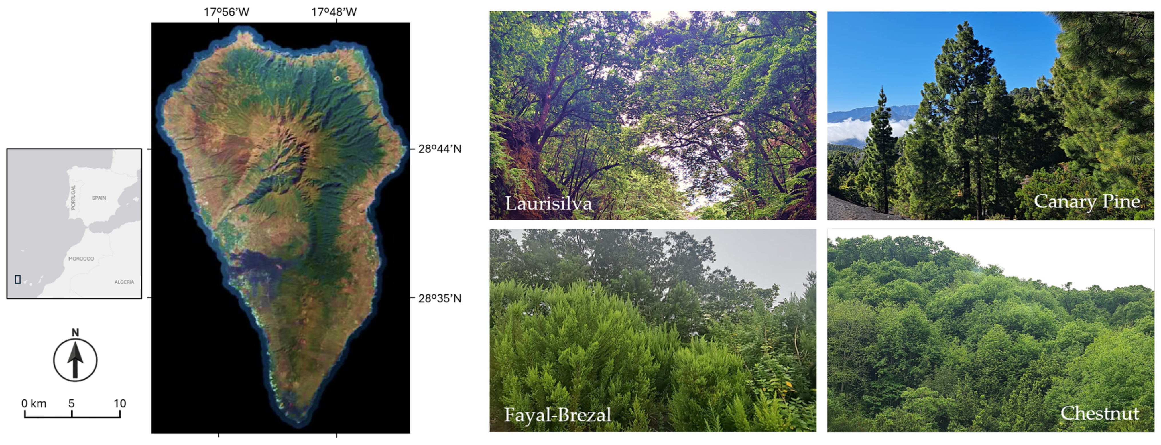
La Palma island exhibits remarkable diversity in its forest formations (Figure 1), resulting from its volcanic origin, steep altitudinal gradients, and the influence of a subtropical oceanic climate. The forest vegetation of La Palma forms a mosaic of high ecological and biogeographical value, characterized by elevated levels of endemism and playing a crucial role in hydrological regulation, soil conservation, and insular biodiversity. These formations are primarily organized into vegetation belts, which are shaped by altitude, exposure to the trade winds, and water availability [28].
In the humid mid-altitudes, particularly on the northern and northeastern slopes, the laurel forest (laurisilva) develops. This relict forest from the Tertiary period features a dense, evergreen canopy dominated by species such as Laurus novocanariensis, Ocotea foetens, Persea indica, and Apollonias barbujana. The understory is rich in ferns, mosses, and epiphytes. Also, sweet chestnut (Castanea sativa) persists on La Palma, primarily as naturalized and semi-naturalized stands, occurring mainly on humid mid-elevation slopes within the laurel forest’s potential range (∼600–1500 m). Although introduced centuries ago, C. sativa now occupies measurable portions of natural habitats [29]. In transitional areas between laurisilva and drier or disturbed environments, the fayal-brezal appears, a secondary forest dominated by Morella faya and Erica arborea. This formation often acts as a successional stage following natural or anthropogenic disturbances and plays a key role in ecological recovery. At higher elevations, roughly between 1200 and 2000 m, the Canary pine forest predominates, dominated almost exclusively by Pinus canariensis, an endemic species with unique fire adaptations, such as thick bark and epicormic sprouting. The pine forest has a relatively open structure and a variable understory composed of xerophytic shrubs and herbaceous species adapted to higher sunlight and thermal amplitude. In the summits and high-mountain zones, above the upper limit of the pine forest, high-altitude shrublands dominate. These ecosystems are adapted to volcanic soils, intense solar radiation, and strong temperature fluctuations, with endemic species such as Spartocytisus supranubius. Finally, in the lower, drier areas, largely altered by human activity, the original thermophilus woodland is present.

2.2. Data

Regarding remote sensing data, high-resolution multispectral imagery, acquired by the WorldView-2/3 satellite and multisensor UAV data were used.
The WorldView satellites provide eight multispectral bands with spatial resolution better than 2 m and 11-bit radiometric resolution [3]. The spectral and spatial specifications are summarized in Table 1. During preprocessing, all multispectral data were resampled to a common spatial resolution of 2 m to ensure consistency among the different scenes.
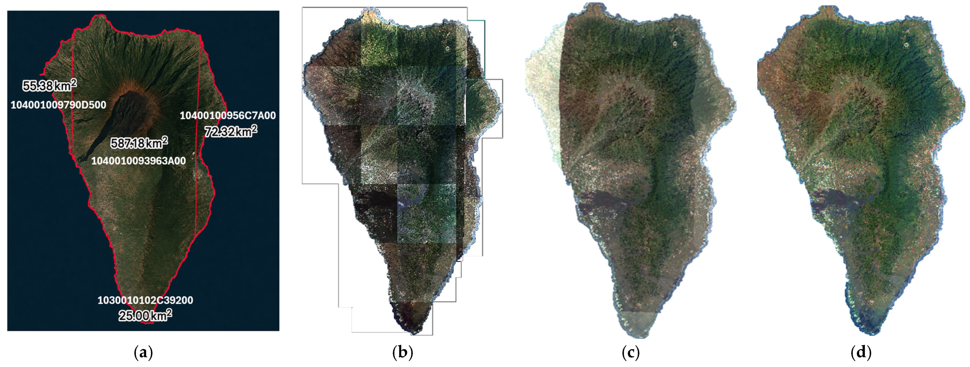
To cover the entire island, four scenes were used to generate the final mosaic. Two scenes, acquired on 4 May 2024, cover 88.3% of the island and almost all the main forested areas. The remaining areas were completed using the closest available cloud-free acquisitions. Table 2 and Figure 2 provide detailed information on each of the scenes used in the final mosaic.
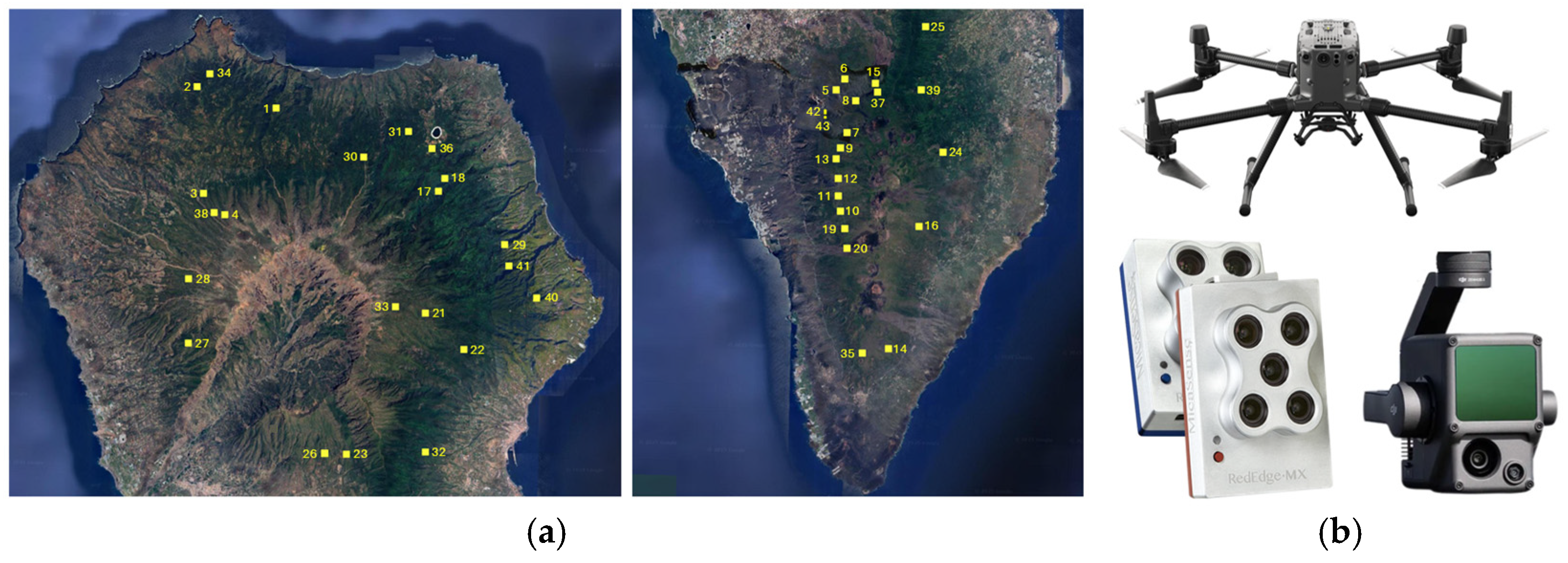
Additionally, UAV data were collected over 43 plots distributed across the island, each covering approximately 9 ha (300 m × 300 m), to obtain detailed vegetation reference information. A DJI Matrice 300 RTK platform (DJI, Shenzhen, Guangdong, China) equipped with a MicaSense RedEdge-MX Dual multispectral sensor (10 bands) was used (MicaSense, Inc., Seattle, WA, USA), providing high radiometric accuracy and narrow spectral bands (Table 1). Furthermore, vegetation height and terrain information were obtained using the Zenmuse L1 sensor (DJI, Shenzhen, Guangdong, China), allowing the acquisition of LiDAR data that facilitate the identification of vegetation species.
In addition, in situ field surveys were conducted in representative plots to identify the species present and to characterize vegetation cover, density, and structure. These field observations were used to support the interpretation and classification of the UAV multispectral and LiDAR data.
The reference cartography was used to identify the spatial distribution of the main forest vegetation types and to support the selection of representative samples for classification (training and testing regions of interest, ROIs). Specifically, cartographic products at island, regional, national, and European scales were reviewed, including vegetation maps from the Government of the Canary Islands (2021), Cabildo of La Palma (PIOLP 2020), Spanish Forest Map (2018), High-Resolution SIOSE (2017), and Corine Land Cover + BackBone (2021). The vegetation map produced by the Government of the Canary Islands, and distributed by GRAFCAN, was selected as the main reference because it is the most detailed and up-to-date product available [28].
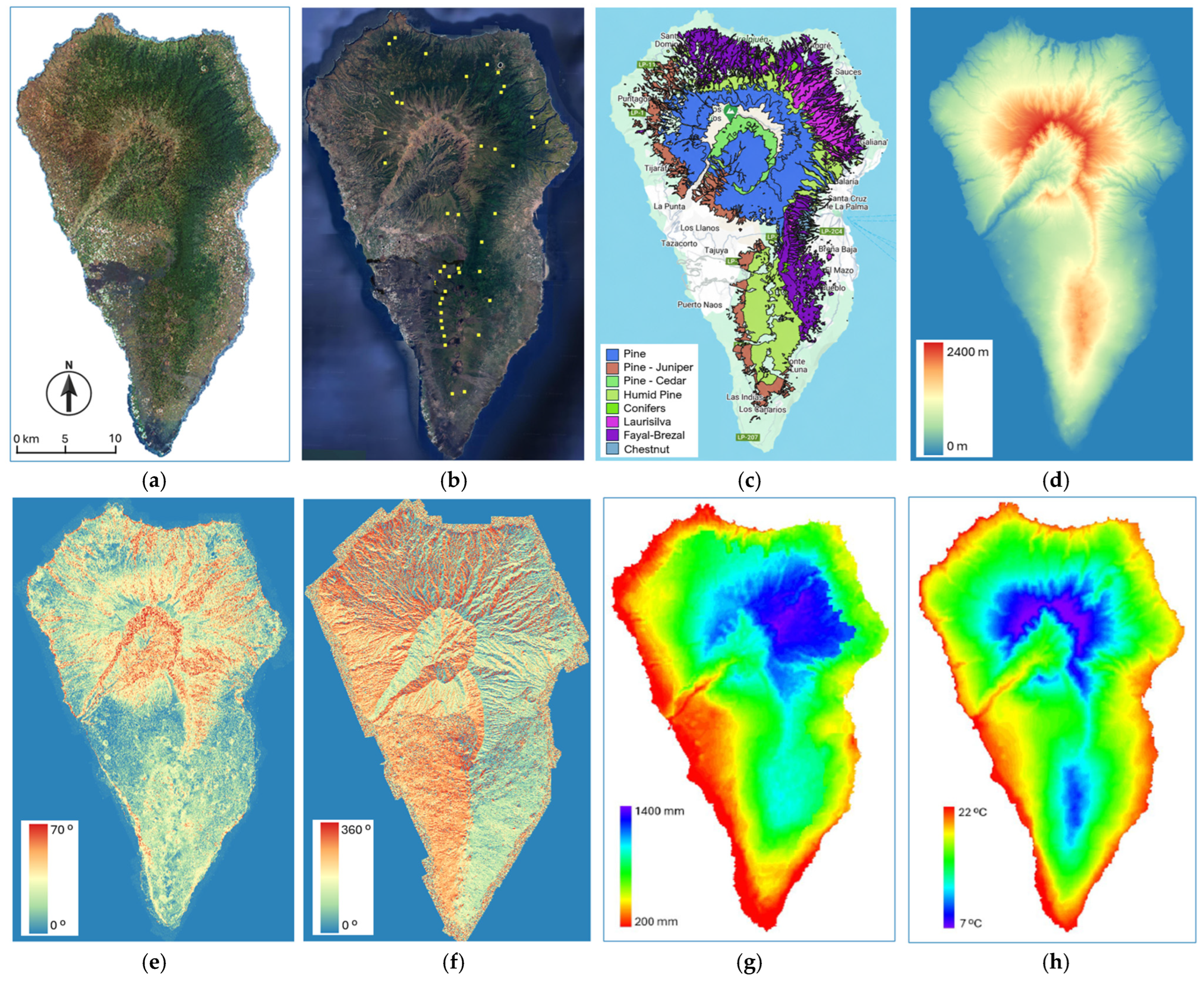
Topographic information of the island was used for geometric corrections and in the classification analysis. Specifically, a high-resolution 2 m Digital Terrain Model (DTM) provided by the National Geographic Institute (IGN) [30] was used, and slope and aspect layers were derived from it. These raster layers were introduced as additional predictor bands together with the WorldView spectral data. Finally, climatic information, including annual precipitation and mean annual temperature from the Canary Islands Climate Atlas [31], was additionally incorporated in the same way. The contribution of these topographic and climatic variables was assessed by comparing the classification accuracy achieved with different combinations of input layers.
Figure 3 shows the remote sensing and auxiliary datasets used in this study. For the UAV data, the location of the 9-ha plots analyzed is displayed. For the climatic data, the selected rainbow color palette was inverted between the two maps to ensure consistency with conventional visual perception; thus, areas with higher precipitation are shown in blue, whereas areas with higher temperatures are represented by reddish tones.

2.3. Processing Methodology

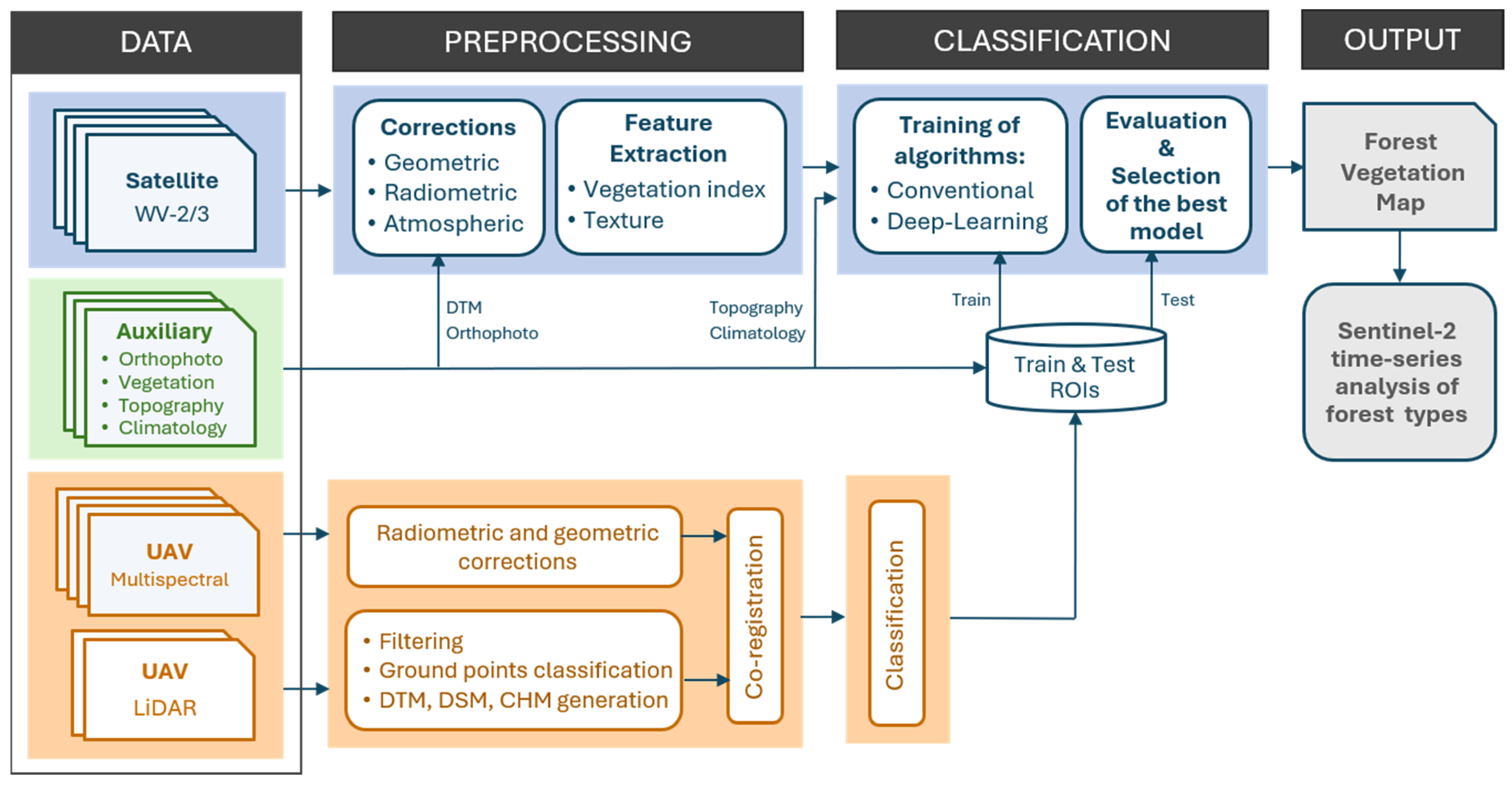
Figure 4 presents a simplified block diagram of the methodological workflow used to evaluate the performance of the classification algorithms and to generate the final forest vegetation map. This schematic overview summarizes the main processing stages, providing a clear visual representation of the analytical framework employed in this study.
Regarding the WorldView imagery, a preprocessing stage was first applied, as multispectral images acquired by spaceborne platforms are affected by several distortions that must be corrected to obtain accurate surface reflectance values [32,33]. Radiometric correction and calibration were applied to adjust sensor digital values and detector performance using the metadata information provided with the images. The atmospheric correction was applied to compensate for absorption and scattering effects in the atmosphere.
In this study, atmospheric correction was performed using the FLAASH (Fast Line-of-sight Atmospheric Analysis of Spectral Hypercubes) model [34]. The model requires information on sensor characteristics, acquisition geometry, surface elevation and atmospheric conditions. Sensor-specific parameters and acquisition metadata (date, time, spatial resolution and illumination conditions) were extracted from the image metadata. The Midlatitude Summer atmospheric model was selected, and a Maritime aerosol model was adopted. The aerosol optical depth (AOD) values at 550 nm were obtained from MODIS products using NASA’s Giovanni platform [35], employing the Combined Dark Target and Deep Blue algorithm for land and ocean [36].
To address the geometric distortions caused by sensor geometry, satellite motion, Earth curvature and terrain relief, geometric corrections were applied. Due to the pronounced relief of La Palma and the oblique viewing geometry of the sensor, each WorldView scene was individually orthorectified using the Rational Polynomial Coefficients (RPCs) provided with the imagery and the 2 m DTM. Following orthorectification, all scenes were further refined through image-to-image registration against a reference orthophoto using a set of well-distributed ground control points. This step ensured precise spatial alignment between scenes acquired on different dates. Multiple WorldView scenes were required to cover the entire island (total area of 708 km2); therefore, orthorectified and registered images were mosaicked into a single composite image. Radiometric consistency across scene boundaries was achieved by applying histogram matching over cloud-free overlap areas.
Upon completion of the preprocessing of the WorldView bands, the supervised classification process was carried out. This process started with the definition of six classes to be discriminated: coniferous forest, laurel forest, fayal-nrezal, chestnut, other vegetation, and soil/others. The first four classes correspond to the target forest vegetation types analyzed in this study. To train and evaluate the classifiers, training and test ROIs were generated as spatially independent and non-overlapping datasets using the reference vegetation map and UAV-derived vegetation maps where available. The ROIs were distributed across the island to capture the variability within each vegetation class. Specifically, they were generated over the WorldView mosaic and a similar number of pixels was selected for each class to avoid class imbalance. On average, approximately 100,000 pixels per class were used for training, while about 10,000 pixels per class were reserved for testing.
Classification performance was evaluated from the confusion matrix using User’s Accuracy (Precision) for each class, Overall Accuracy (OA), and the Kappa coefficient. User’s Accuracy was calculated as the proportion of correctly classified pixels for a given class relative to all pixels classified as belonging to that class, while OA represents the proportion of correctly classified pixels relative to the total number of test pixels.
Spectral separability between class pairs was analyzed using the Jeffries–Matusita distance [37], which is bounded by 2, where values above 1.8 typically indicate good class discrimination.
Two approaches were evaluated to assess the performance of the different algorithms:
(i)
Conventional supervised classification algorithms. Specifically, nine classifiers were evaluated [38]: Minimum Distance (MD), Mahalanobis Distance (MhD), Parallelepiped (P), Spectral Angle Mapper (SAM), Maximum Likelihood (ML), Naïve Bayes (NB), K-Nearest Neighbors (KNN), Random Forest (RF), and Support Vector Machine (SVM).
(ii)
An artificial intelligence approach based on deep learning. The SegFormer model [16] was selected because of its good trade-off between accuracy and computational efficiency for large-area very-high-resolution image classification. It is an encoder–decoder transformer-based architecture that combines an efficient hierarchical encoder with a lightweight decoder, capturing both local details and global context while handling high resolutions and spatial variability without heavy convolutions.
The network was fine-tuned using a random selection of 30% of the available training pixels from each land-cover class. However, the same spatially independent test ROIs were used for the evaluation of all classifiers. During this process, the weights of both the encoder and the decoder were updated. The pretrained backbone provides generalizable feature representations, while fine-tuning allows the model to adapt specifically to the spatial patterns, textures, and spectral signatures present in the study area. Before each forward pass, a normalization step is applied using fixed mean and standard-deviation tensors, ensuring stable input distributions throughout the training process. To improve the robustness and generalization capability of the SegFormer model, on-the-fly data augmentation was applied during training. Specifically, random rotations, random flips, and spectral noise addition were used. The model was trained for 50 epochs using a learning rate of 6 × 10⁻⁵, a batch size of 64, and input patches of 5 × 5 pixels.
The traditional and machine-learning classifications were performed using ENVI 6.2, while the SegFormer model was implemented in Python 3.8.10 using the PyTorch 1.10.1 framework.
To improve classification results, in addition to spectral bands, the inclusion of derived features (such as the vegetation index WDRVI and textural parameters), topographic information (DTM, slope, and aspect), and climatic variables (temperature and precipitation) was evaluated.
The Wide Dynamic Range Vegetation Index (WDRVI) has proven to be a robust and reliable indicator of vegetation status, particularly in areas with moderate to high biomass [37]. Unlike traditional indices such as NDVI, WDRVI enhances sensitivity in dense vegetation canopies by reducing saturation effects, allowing for improved discrimination of vegetation vigor and structural variations. This characteristic makes WDRVI especially suitable for detailed vegetation analysis and monitoring, providing more accurate information on canopy condition and spatial heterogeneity. The mathematical formulation of the WDRVI is as follows [37]:
W D R V I = 0.2   ×   N I R R E D 0.2   ×   N I R + R E D
where NIR represents the reflectance in the near-infrared band, RED corresponds to the reflectance in the red band, and 0.2 is a weighting coefficient used to reduce saturation effects.
Texture information was derived using the gray-level co-occurrence matrix (GLCM) computed on the first principal component obtained from the PCA transformation of the eight WorldView spectral bands [39]. From the GLCM, the eight Haralick texture features were extracted, namely, mean, variance, homogeneity, contrast, dissimilarity, entropy, second moment (angular second moment), and correlation. These parameters characterize different aspects of spatial gray-level relationships and textural heterogeneity. Nevertheless, a high degree of redundancy was observed among most of the extracted features; therefore, variance was selected as the most informative and representative texture descriptor for subsequent analyses.
In summary, the complete non-climatic input combination to the classifiers (MS + WDRVI + Texture + DTM + Slope + Aspect) contained 13 features. When precipitation and temperature were additionally included, the maximum number of input features was 15.
Following the methodology outlined in Figure 4, the information derived from the UAV campaigns over the 43 plots (300 × 300 m each), shown in Figure 3b, was used to support the generation of training and test regions for each land-cover class. Two complementary UAV-based data acquisitions were conducted: one using a MicaSense multispectral sensor and another employing a Zenmuse LiDAR system. These multisensor datasets provided high-resolution spectral and structural information that was essential for accurately delineating representative samples of the different forest vegetation types. Appendix A summarizes the preprocessing steps performed on the UAV sensor data. For the LiDAR dataset, standard preprocessing steps were applied to derive both the Digital Terrain Model (DTM) and the Canopy Height Model (CHM) [40]. Regarding the multispectral imagery, the raw data were corrected using the typical radiometric, atmospheric, and geometric procedures [33]. In addition, an automatic co-registration workflow was implemented to ensure spatial alignment between the multispectral layers and the LiDAR-derived models. Ground control points were also incorporated to further improve spatial accuracy and guarantee precise matching of both datasets. All UAV-derived products and the WorldView imagery were referenced to the same coordinate system (WGS 84/UTM zone 28N), allowing their direct spatial matching. Once the preprocessing steps were completed, the combined multispectral and LiDAR information served as the input for a robust supervised classification approach. Specifically, a Support Vector Machine (SVM) classifier was employed due to its well-known capacity to handle high-dimensional feature spaces and its effectiveness with limited training samples. Random Forest was also evaluated; however, in this case, it achieved slightly lower performance.
The resulting classification output generated detailed maps of forest vegetation types, which were used as high-resolution reference information to identify the vegetation classes present within the UAV plots. The ROIs used for the UAV classification were different from those subsequently defined for the WorldView classification. New WorldView training and test ROIs were independently delineated over the WorldView mosaic, using the UAV-derived maps as reference information, where available, without pixel-to-pixel transfer of the 10 cm UAV classification maps to the 2 m WorldView. Additional ROIs were selected, for the WorldView classification, in other areas of the island to capture the spatial, topographic, and within-class variability of the different forest vegetation types.
Finally, to illustrate the potential of the derived forest vegetation map for temporal monitoring of the main forest types of the island, a Sentinel-2 vegetation index time series was generated for the period 2019–2025. Sentinel-2 Level-2A images were used, which are provided as corrected surface reflectance products. For each month, the available cloud- and shadow-free acquisitions were selected to generate a monthly image. The forest vegetation map obtained in this study was then used to delimit each forest type and analyze its temporal evolution separately.

3. Results

This section summarizes the most significant results of the study, emphasizing the main outcomes derived from the implemented workflow.

3.1. WorldView Preprocessing

To increase revisit frequency, WorldView satellites are designed with pointing agility, allowing images to be acquired at substantial off-nadir viewing angles. However, this capability introduces geometric distortions and degrades the effective spatial resolution. As shown in Table 2, the available scenes for La Palma were acquired with relatively high off-nadir angles. As a result, the application of geometric correction and orthorectification techniques was critical to ensure the spatial accuracy of the data. This requirement is especially important given the complex topography of La Palma, characterized by steep slopes and pronounced elevation changes, which further amplify geometric distortions in off-nadir satellite imagery.
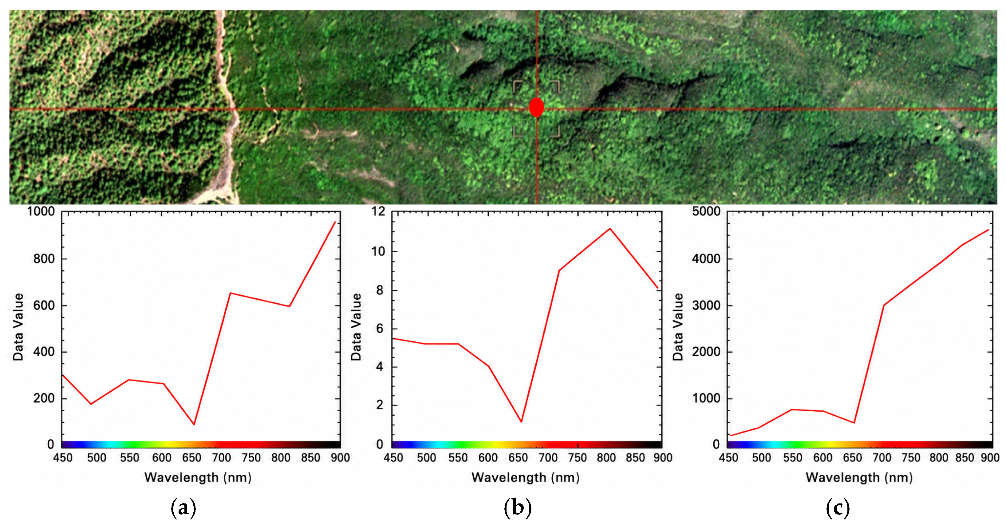
As indicated in Section 2.3, radiometric calibration and atmospheric correction were applied to the imagery. For the atmospheric correction, the FLAASH radiative transfer model was used and the parameters described in that section were selected. In particular, the atmospheric visibility was computed from the aerosol optical depth data obtained for each acquisition date. For example, an AOD value of 0.084 resulted in an estimated visibility of 93.15 km for the 4 May 2024 scenes, which were representative of the atmospheric conditions for most of the area used in the mosaic. Following the application of both corrections, image pixels can be considered to accurately represent surface reflectance values. Figure 5 shows an example of a vegetation pixel before and after the correction process, highlighting the improvement achieved in retrieving surface-level reflectance. It can be appreciated that, after the atmospheric correction, the spectral signature conforms to the typical behavior of vegetated surfaces. Reflectance values in the visible region are characterized by low responses in the blue and red bands and a relative maximum in the green band. In contrast, the near-infrared region exhibits high reflectance values, consistent with the strong scattering associated with healthy vegetation canopies.
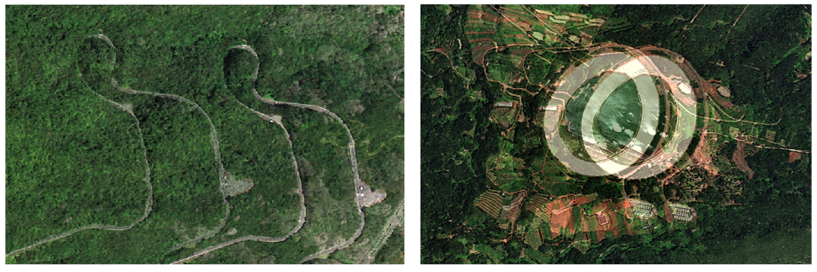
As indicated, very-high-resolution satellite imagery is affected by geometric distortions that hinder accurate geolocation and spatial comparison between datasets. Therefore, geometric correction is a critical preprocessing step for WorldView imagery, especially in areas with complex topography, as in La Palma. After geometric correction, orthorectification, registration and mosaicking, the resulting WorldView images were accurately geolocated and spatially consistent, allowing reliable multitemporal analysis and integration with other geospatial datasets. To illustrate the magnitude of the geometric variations, Figure 6 compares the original image with the image after orthorectification and geolocation. Both images were overlaid using transparency, before and after geometric corrections, in order to clearly visualize the spatial differences introduced by the correction process.

3.2. Classes

In accordance with the island’s conservation authorities, a set of vegetation classes was selected to represent the main forest vegetation types considered in the study (Figure 1):
  • Pine forest/coniferous;
  • Laurisilva (L);
  • Fayal-brezal (F-B);
  • Chestnut (C);
  • Other vegetation (OV);
  • Soil and others (S&O).
The “soil and others” class includes all remaining land-cover types, such as non-vegetated soil, built-up areas, asphalt, water bodies, and shadowed areas.
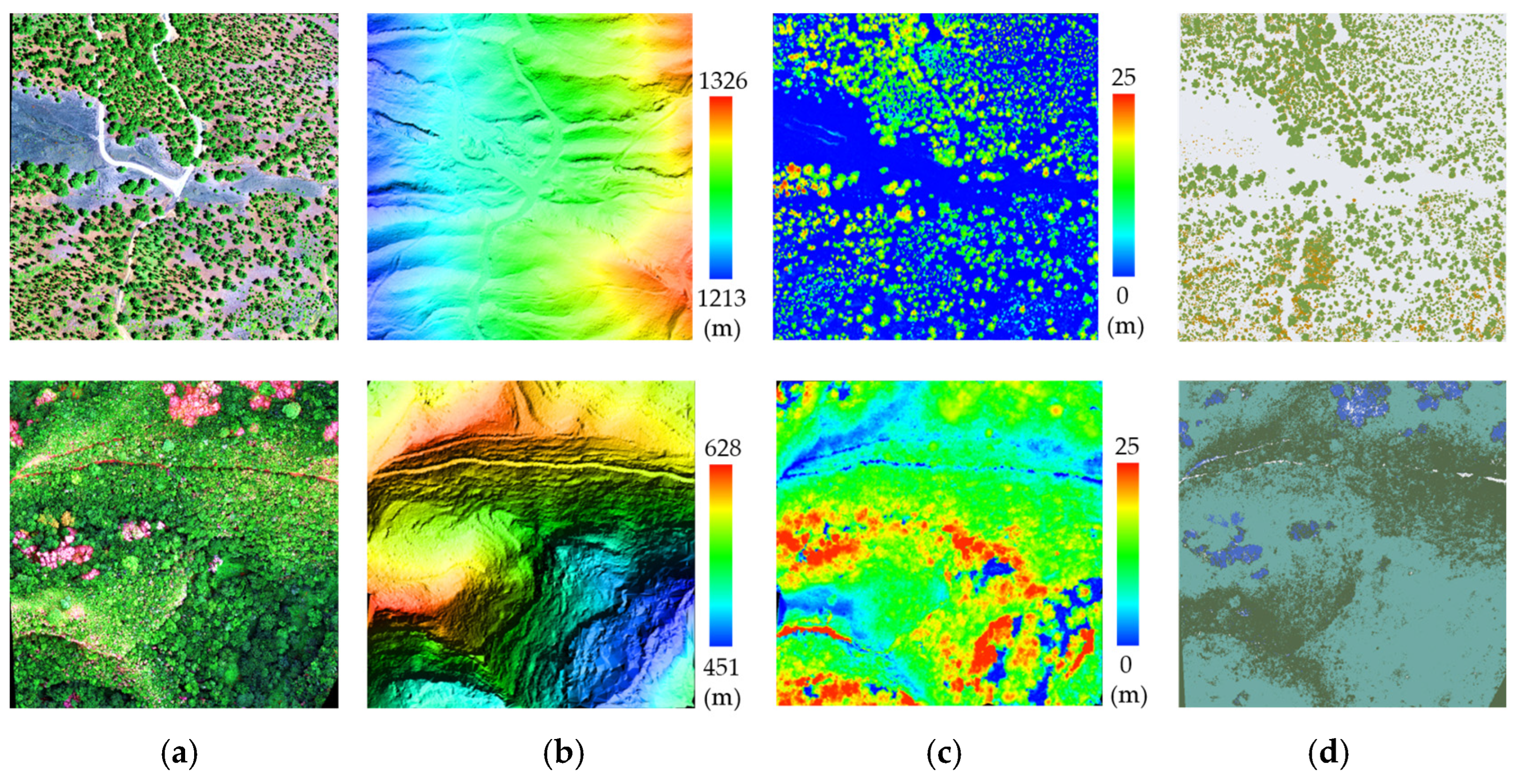
The vegetation map from the Canary Islands Government was used as the main reference for defining the WorldView training and test samples. In areas covered by the UAV surveys, the UAV vegetation maps (Figure 7 and Appendix A for further details) were used only as auxiliary high-resolution information to support the delineation and verification of WorldView samples. These UAV classification maps were not used as direct input to the WorldView classifiers.
A spectral separability analysis was conducted for each pair of classes using the Jeffries–Matusita (JM) distance as the separability metric. As previously noted, values close to 2 indicate good class separability, whereas lower values reflect higher spectral similarity and, consequently, a greater likelihood of confusion during classification. The results are summarized in Table 3, where the lowest separability values were observed between the laurisilva and fayal-brezal classes. Poor spectral separability was also found between the other vegetation class and both the chestnut and coniferous classes. As expected, the best separability was obtained between the soil/others class and the remaining vegetation classes.

3.3. Conventional Supervised Classifiers

A comparative analysis of classifiers was performed and the supervised classifier achieving the highest accuracy was identified using two input datasets: (1) MS: the eight WorldView-2 multispectral bands, and (2) All: multispectral bands plus derived features (vegetation index and texture) and topographic data (DTM, slope, and aspect).
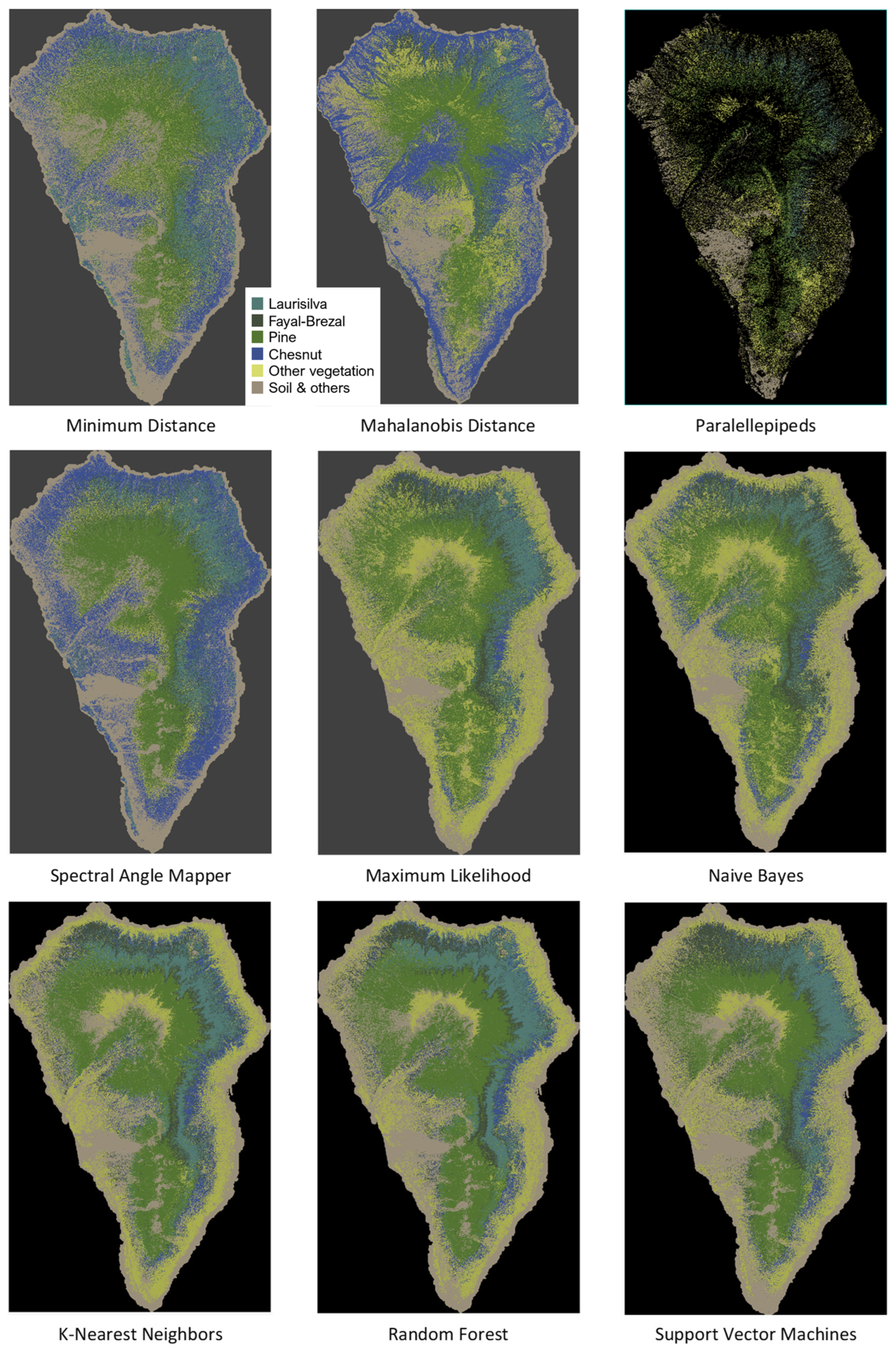
Table 4 and Figure 8 present the results obtained for the nine classifiers assessed. SVM, RF and Maximum Likelihood provided the highest accuracies. Based on accuracy and computational efficiency, the Random Forest classifier was selected. Next, a more detailed analysis was conducted for this classifier using different input combinations, including annual accumulated precipitation and mean temperature maps (Figure 3g,h). As shown in Table 5, results were generally similar; however, the combination of multispectral bands, vegetation index, slope, and aspect yielded the best performance for the target classes. The inclusion of temperature or precipitation did not improve classification accuracy.

3.4. Deep Learning–Based Classifier

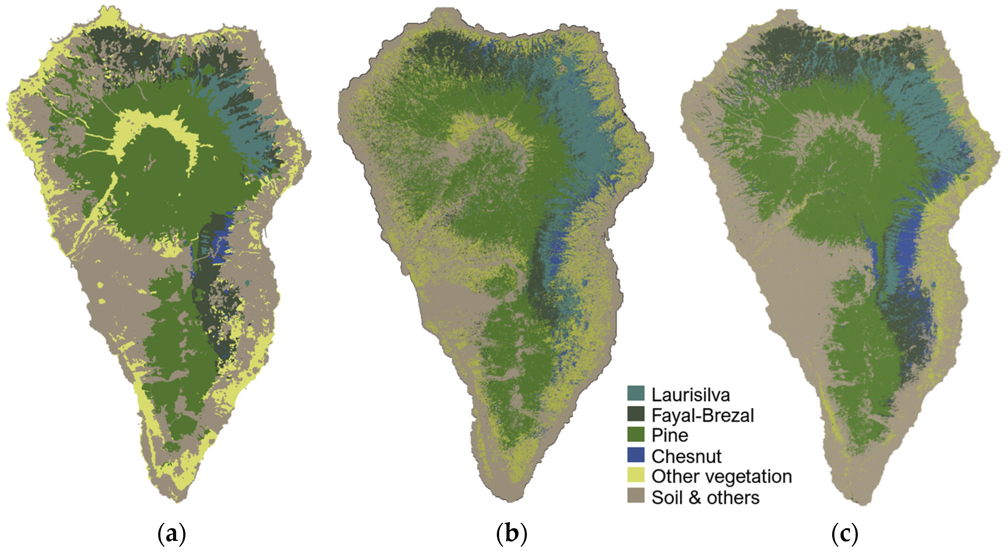
The map of the most representative forest vegetation types obtained with the fine-tuned SegFormer model using the 13-feature input combination (8 WorldView bands + WDRVI + texture + DTM + slope + aspect) is shown in Figure 9c. The map generated with Random Forest using the same input is also included for comparison. Visually, the SegFormer results are generally consistent with the reference map, although some discrepancies are observed in the Other Vegetation class. It should be noted that the reference map represents vegetation at the stand or dominant vegetation-unit level, rather than at the individual plant level. Moreover, the Other Vegetation class is inherently more dynamic, since herbaceous plants may be drier at the WorldView image acquisition date. This seasonal effect may increase spectral variability within this class and partly explain the discrepancies observed between the reference map and the satellite-derived classification.
The quantitative assessment computed over the same test regions (Table 6) shows that SegFormer outperformed the machine-learning models for most dominant cover types, with the exception of chestnut stands. However, the overall accuracy metrics were slightly lower than those obtained with Random Forest, mainly due to the lower accuracy achieved for the soil/other class.

3.5. Sentinel-2 Time-Series Analysis of Forest Vegetation Types

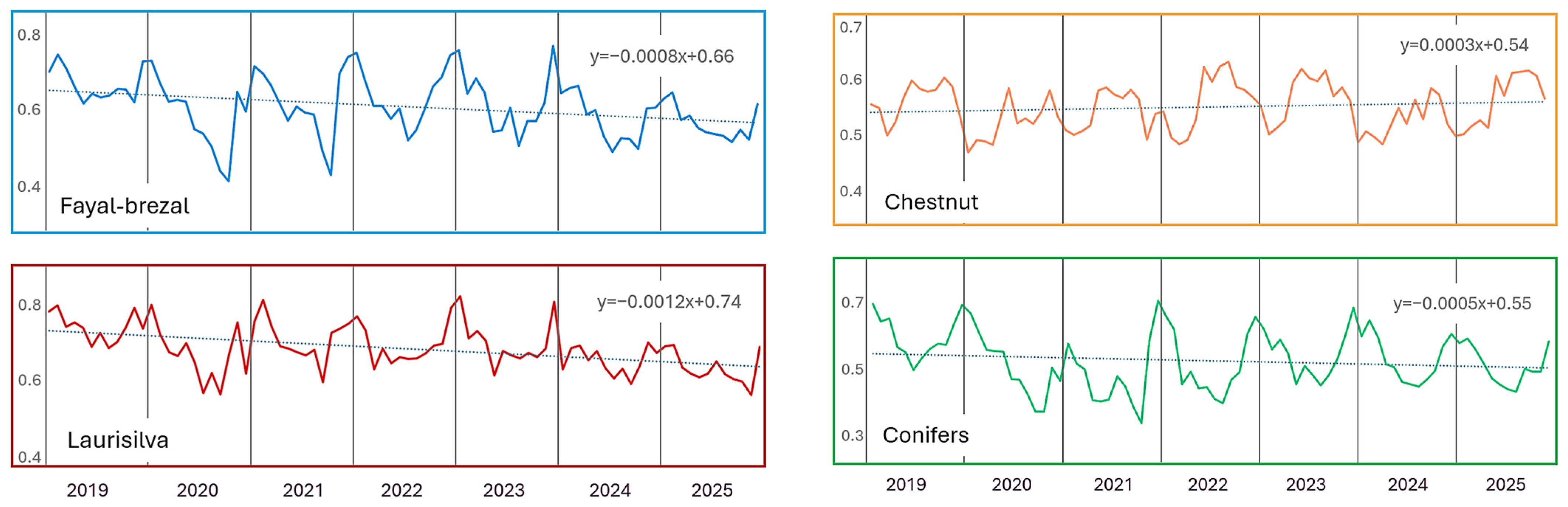
By combining Sentinel-2 imagery with the high-resolution vegetation classification derived from WorldView data, it has been possible to analyze the temporal variation in each vegetation type at the island-wide scale. This approach allows a more detailed understanding of habitat dynamics, providing a robust basis for monitoring forest health and conservation status. An illustrative example is included in Figure 10, where a seven-year time series (2019–2025) of the vegetation index was generated to assess the state of conservation of different forest vegetation types across the island. Overall, the fitted trends indicate slight decreases in the vegetation index for laurisilva, fayal-brezal, and pine forest, whereas chestnut stands show a slight increase. In all cases, these long-term trends are modest compared with the marked seasonal and interannual variability observed throughout the study period.

4. Discussion

4.1. Data and Preprocessing Challenges

This study focuses on the analysis of forest vegetation using high spatial resolution multispectral satellite data. Several challenges were addressed to get the desired information. The main difficulty was obtaining suitable imagery for this study for several reasons. First, the prevalence of cloud cover over La Palma. While the Canary Islands as a whole experience frequent cloud intervals on the windward (northern) slopes of the major islands due to trade wind regimes, this effect is especially pronounced over La Palma’s rugged terrain, making it difficult to find cloud-free scenes that cover the entire study area simultaneously. In addition, it was essential to select images acquired during months with relatively high solar elevation angles, as acquisitions in autumn or winter result in extensive shadowed areas due to the island’s steep topography. Furthermore, only a limited number of images fulfilling these requirements are available in the WorldView archive, and most of them do not provide full coverage of the island. This combination of constraints further increases the difficulty of obtaining a single, cloud-free, and geometrically suitable dataset covering the entire study area.
As indicated, the study area considered in this work covers a relatively large spatial extent, approximately 700 km2, which represents a significant challenge when using very high spatial resolution satellite imagery. In the existing literature, only a limited number of studies address areas of this magnitude, as most applications are restricted to regions of 100 km2 or less. This limitation is mainly driven by the high economic cost associated with the acquisition of high-resolution satellite data, as well as by the increasing complexity of the preprocessing workflow as the number of required scenes grows. In particular, the generation of large-area mosaics from multiple satellite scenes involves substantial radiometric challenges. For instance, a recent work [41] highlights the radiometric inconsistencies arising from differences in acquisition dates and observation geometries among the individual scenes composing the final mosaic. Such differences can lead to significant heterogeneity that, if not properly corrected, hinders the performance of image classification algorithms applied to the full dataset. When individual scenes exhibit different radiometric levels, achieving a consistent and reliable classification over the entire mosaic becomes particularly difficult.
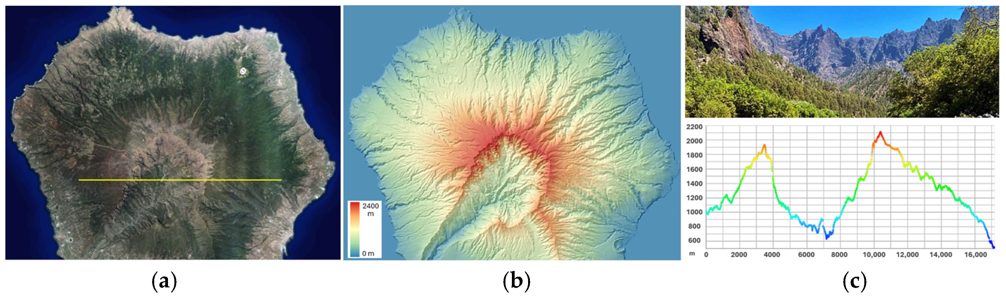
These radiometric challenges are further exacerbated in the present study by the pronounced topographic complexity of La Palma. This extreme relief introduces strong geometric distortions in satellite imagery when acquisitions are performed with high off-nadir viewing angles. Additionally, most of the study area was imaged with off-nadir angles of approximately 28°, which significantly increases geometric deformation effects and necessitates accurate correction. Consequently, image orthorectification required the use of a high-resolution digital terrain model with a spatial resolution of 2 m covering the entire island. Commonly, elevation models with coarser spatial resolutions of several meters are considered but are not suitable under such topographic conditions, as they may introduce substantial geometric errors. Figure 11 presents the generated DTM together with a representative topographic profile from the Caldera de Taburiente area, clearly illustrating the terrain complexity and the scale of the geometric corrections required. In particular, the topographic profile of the Caldera de Taburiente area shows elevation differences exceeding 1.5 km with extremely steep slopes approaching vertical conditions.

4.2. Classification Performance

Regarding classification performance, Random Forest and Support Vector Machine provided the best overall results among the conventional classifiers evaluated in this study. Using the full set of spectral, derived, and topographic features, RF achieved an overall accuracy of 77.5%, compared with 73.8% for SVM, respectively. These results are consistent with the general findings reported in a recent meta-analysis [5], which showed that RF and SVM are among the most robust classifiers in remote sensing applications and that their relative performance depends strongly on the characteristics of the dataset and classification problem.
It should also be noted that the reference vegetation map represents dominant vegetation units rather than individual trees or plants, while detailed UAV-derived reference information was available only for the surveyed plots. These factors should be considered when interpreting class-specific classification accuracy.
Quantitative comparison with previous studies provides useful context, although accuracy values should be interpreted with caution because classification performance depends on several factors, including the number and definition of classes, spatial and spectral resolution, heterogeneity of the study area, input features, training samples, and validation strategy. For example, ref. [42] reported an overall accuracy of approximately 82% for the classification of ten tree species using Random Forest and WorldView-2 imagery. A forest habitat mapping study [43], using Sentinel-1, Sentinel-2, and topographic information, reported overall accuracies ranging from 91.03% to 94.04% for three areas. These values are higher than those obtained in the present study, but they are not directly comparable. In the present case, the classification was performed over a large and highly heterogeneous island, including spectrally similar forest types and transitional vegetation communities. Other comparative studies [44,45,46] using medium- and high-resolution satellite data have also shown that both SVM and RF can achieve high overall accuracies in land cover mapping, with SVM sometimes exhibiting better performance when training sample sizes are small and class separability is high, while RF tends to be more robust when handling large datasets and heterogeneous spectral variability.
Regarding the deep-learning approach, previous studies have also shown that, despite the strong performance reported for SegFormer in several remote sensing applications, as detailed in the Introduction, transformer-based segmentation models do not universally outperform classical machine learning or convolutional neural network approaches. One of the main limitations arises in scenarios with limited training samples, where models such as RF or SVM often remain more robust due to their lower data requirements and reduced risk of overfitting [44,47]. Several comparative works in land cover and agricultural mapping have reported cases where classical methods or CNN-based architectures slightly outperform transformer-based models when annotated data are scarce or highly imbalanced [48,49,50]. In this study, SegFormer achieved an overall accuracy of 75.5% when all relevant input features were included. Although its global accuracy was slightly lower than that obtained with RF, SegFormer achieved higher class-specific accuracies for laurisilva (77.4% vs. 75.7%), fayal-brezal (62.3% vs. 44.2%), pine forest (84.6% vs. 79.8%), and other vegetation (84.6% vs. 78.4%). Nevertheless, deep learning approaches are more complex and generally require larger and more representative training datasets.

4.3. Auxiliary Data and Ecological Interpretation

The results show that adding ancillary information does not improve all classifiers in the same way. The complete set of non-climatic features increased the overall accuracy of RF from 76.1% to 77.5%, while larger improvements were obtained for ML, NB, and KNN. In contrast, SVM showed almost no improvement, and some classifiers performed worse when the additional features were included. For RF, precipitation and temperature reduced the overall accuracy. Conversely, SegFormer showed a stronger benefit from the additional features, increasing overall accuracy from 58.1% to 75.5%. These results indicate that adding more variables does not necessarily lead to higher accuracy and that the usefulness of ancillary information depends on its relationship with the spatial and ecological distribution of each vegetation type. A further methodological consideration concerns the use of aspect in its original 0–360° representation. Since aspect is a circular variable, alternative representations based on the joint use of sine and cosine components should be evaluated in future studies.
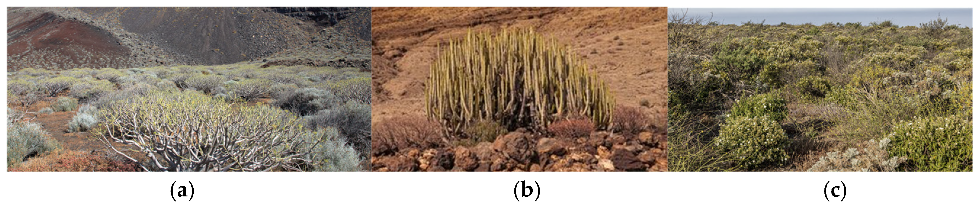
The classification results highlight that some vegetation types were particularly difficult to discriminate in La Palma due to their ecological and structural characteristics. This is especially the case for the fayal–brezal formation, which is often combined with laurel forest (laurisilva) stands, forming transitional zones and mixed canopies. These two formations share similar spectral responses in multispectral imagery, partly due to comparable leaf traits and canopy structures, which complicates their separation using spectral information alone. The most challenging class, however, corresponds to “other vegetation”, which encompasses a wide range of shrub and herbaceous communities. This class is highly heterogeneous, with phenological stages that can vary significantly depending on the acquisition date, leading to substantial intra-class spectral variability. In addition, many of these vegetation elements are small in size, in some cases smaller than the satellite ground sampling distance, which increases spectral mixing with surrounding bare soil and further hampers accurate classification. As an example, Figure 12 illustrates typical shrub species, highlighting the complexity of this class.
Despite these limitations, in insular forest ecosystems, where habitats are often spatially fragmented and include species and communities of high conservation value, detailed spatial information is essential to support effective monitoring. Recent Earth observation studies [51] have highlighted the potential of satellite archives and time-series analysis for characterizing forest disturbances over large spatial and temporal scales. In this context, an illustrative example of the main applications of this work is presented in Figure 10, going beyond mapping the distribution and area occupied by the dominant forest vegetation types. By combining Sentinel-2 time series with the high-resolution WorldView-derived classification, temporal variations in vegetation indices can be analyzed separately for each dominant forest type, both at an island scale and in specific areas of interest. Although vegetation indices alone do not provide a comprehensive assessment of forest health, they provide useful indicators of vegetation vigor and temporal change that can support longer-term forest monitoring.

5. Conclusions

This study demonstrates the potential of very-high-resolution multispectral satellite imagery combined with advanced classification techniques for detailed forest vegetation mapping over large and topographically complex areas. Using WorldView data, complemented by UAV-based multispectral and LiDAR information as auxiliary high-resolution reference data, it was possible to generate an accurate and spatially consistent map of the main forest vegetation types of La Palma island, despite the challenges posed by rugged terrain, frequent cloud cover, and radiometric inconsistencies among multiple satellite acquisitions.
The comparative analysis showed that RF and SVM were among the best-performing conventional classifiers, with RF achieving the highest overall accuracy. The effect of adding ancillary information depended on both the classifier and the forest class. For several conventional classifiers, the inclusion of vegetation, texture, and topographic information produced moderate improvements, although this effect was not consistent across all algorithms. In the case of RF, climatic variables did not improve the overall classification accuracy. In contrast, SegFormer benefited more clearly from the additional features, although deep learning approaches require higher computational resources and more extensive and balanced training datasets.
Beyond static mapping, the forest classification derived in this work provides a valuable baseline for monitoring temporal changes in forest extent and condition. When combined with medium-resolution time series data, such as Sentinel-2 imagery, this approach enables the assessment of vegetation dynamics and the detection of disturbances caused by wildfires, volcanic eruptions, and climate-related stressors in the main habitats considered. Overall, this study provides practical evidence for selecting suitable classifiers and input information for detailed forest monitoring and supports forest management and conservation in vulnerable island ecosystems.
Future research will focus on evaluating more advanced deep learning architectures and testing foundation models. These approaches may better capture both local spatial details and long-range contextual information, which is particularly relevant in heterogeneous forest landscapes. Future work will also explore the integration of LiDAR canopy height models as an additional input feature for the classifier. The incorporation of structural and height-related information is expected to improve the discrimination of spectrally similar or transitional forest classes, thereby supporting the generation of more accurate and robust forest vegetation maps.

Author Contributions

Conceptualization, J.M. and F.E.; methodology, All authors; software, J.M., A.M.-B., Á.G.-P. and M.B.; validation, J.M., A.M.-B., C.G.-M., Á.G.-P. and M.B.; formal analysis, J.M., A.M.-B. and Á.G.-P.; investigation, All authors; resources, F.E.; data curation, J.M., A.M.-B., Á.G.-P. and M.B.; writing—original draft preparation, J.M.; writing—review and editing, F.E., A.M.-B., C.G.-M. and Á.G.-P.; visualization, J.M., A.M.-B. and Á.G.-P.; supervision, J.M., F.E. and C.G.-M.; project administration, F.E.; funding acquisition, J.M. and F.E. All authors have read and agreed to the published version of the manuscript.

Funding

This research was funded by the Ministry for the Ecological Transition and the Demographic Challenge of the Government of Spain (Real Decreto-ley 20/2021 de 5 de octubre; 1207 456E 7600400 fondo 70V1201 227G0170), the Government of the Canary Islands (Orden de 22 de junio de 2022), and the Island Council of La Palma, within the framework of the project ‘Study of the effects of the La Palma volcanic eruption on threatened species and their natural habitats’. The project was entrusted to GESPLAN, S.A. (ref. 316/2023/ACU).

Data Availability Statement

The WorldView-2/3 datasets presented in this article are not readily available because a single user license was purchased.

Acknowledgments

We would like to express our sincere gratitude to GESPLAN and the Island Council of La Palma for their support regarding the forest vegetation of interest on the island (project ref. 316/2023/ACU). We also acknowledge the availability of the high-resolution digital terrain model (2 m) generated from the LiDAR flights of the second coverage of the National Aerial Orthophotography Plan and provided by the Spanish National Geographic Institute. We further acknowledge the availability of the precipitation and temperature maps obtained from the Canary Islands Climate Atlas, as well as the orthophotos supplied by the Government of the Canary Islands and accessible via the GRAFCAN platform. During the preparation of this manuscript, the author used ChatGPT-5.6 to improve the written quality and formatting of the text and to improve the quality or resolution of some figures (Figure 2, Figure 5, Figure 6, Figure 7, Figure 11 and Figure A2). The authors have reviewed and edited the output and take full responsibility for the content of this publication.

Conflicts of Interest

The authors declare no conflicts of interest.

Abbreviations

The following abbreviations are used in this manuscript:
AODAerosol Optical Depth
CHMCanopy Height Model
CNNsConvolutional Neural Networks
DL Deep Learning
DTMDigital Terrain Model
DSMDigital Surface Model
FLAASHFast Line-of-sight Atmospheric Analysis of Spectral Hypercubes
GLCMGray-Level Co-occurrence Matrix
GSDGround Sampling Distance
JM Jeffries–Matusita (distance)
KNNK-Nearest Neighbors
LiDARLight Detection and Ranging
MDMinimum Distance
MhDMahalanobis Distance
MLMaximum Likelihood
NB Naïve Bayes
NDVINormalized Difference Vegetation Index
PCAPrincipal Component Analysis
RF Random Forest
ROIRegion of Interest
RPCRational Polynomial Coefficients
SAMSpectral Angle Mapper
SVMSupport Vector Machine
TINTriangular Irregular Network
UAVUnmanned Aerial Vehicle
VI Vegetation Index
VHRVery High Resolution
WDRVIWide Dynamic Range Vegetation Index

Appendix A

To obtain accurate information on forest vegetation, a detailed analysis was conducted at 43 locations using data acquired by a UAV equipped with a multispectral sensor and a LiDAR system (Figure A1). In order to enable a multimodal analysis with the LiDAR data, all multispectral bands were resampled to a spatial resolution of 10 cm. In addition, for several of the surveyed plots, an exhaustive field campaign was conducted to collect forest inventory data, as well as detailed information on vegetation density and structural characteristics.
Figure A1. (a) Location of the UAV survey plots and (b) DJI Matrice 300 RTK drone equipped with a MicaSense RedEdge-MX Dual multispectral sensor and a Zenmuse L1 LiDAR system.
Remotesensing 18 02871 g0a1
The processing workflow applied to the UAV data is shown in Figure 4. In addition to standard radiometric and geometric corrections, the most relevant preprocessing step applied to multispectral data was the co-registration with the LiDAR dataset, ensuring spatial overlap and accurate georeferencing. Since the Zenmuse L1 system integrates both a LiDAR sensor and an RGB camera, it was possible to apply a semi-automatic registration procedure. This approach initially derived control points by estimating the similarity between both datasets using the green band and applying a cross-correlation algorithm within moving windows. Subsequently, heat maps were generated to support the manual identification, inclusion, or removal of outliers, providing a spatial indication of the distance between corresponding feature points in both images.
On the other hand, LiDAR data processing included outlier filtering followed by ground point classification for the generation of digital models (DTM, DSM and CHM). One of the most critical steps in the point cloud preprocessing is ground point classification. The separation between ground and non-ground classes enables the accurate generation of the Digital Terrain Model, which constitutes a fundamental basis for subsequent processing. Several algorithms have been developed for ground classification when the data provider does not supply pre-classified point clouds, as is the case in this study. After reviewing and evaluating different methods (e.g., Progressive Morphological Filter, Cloth Simulation Function, Triangular Irregular Network) [52,53,54], the Progressive TIN (Triangular Irregular Network) densification filter was selected.
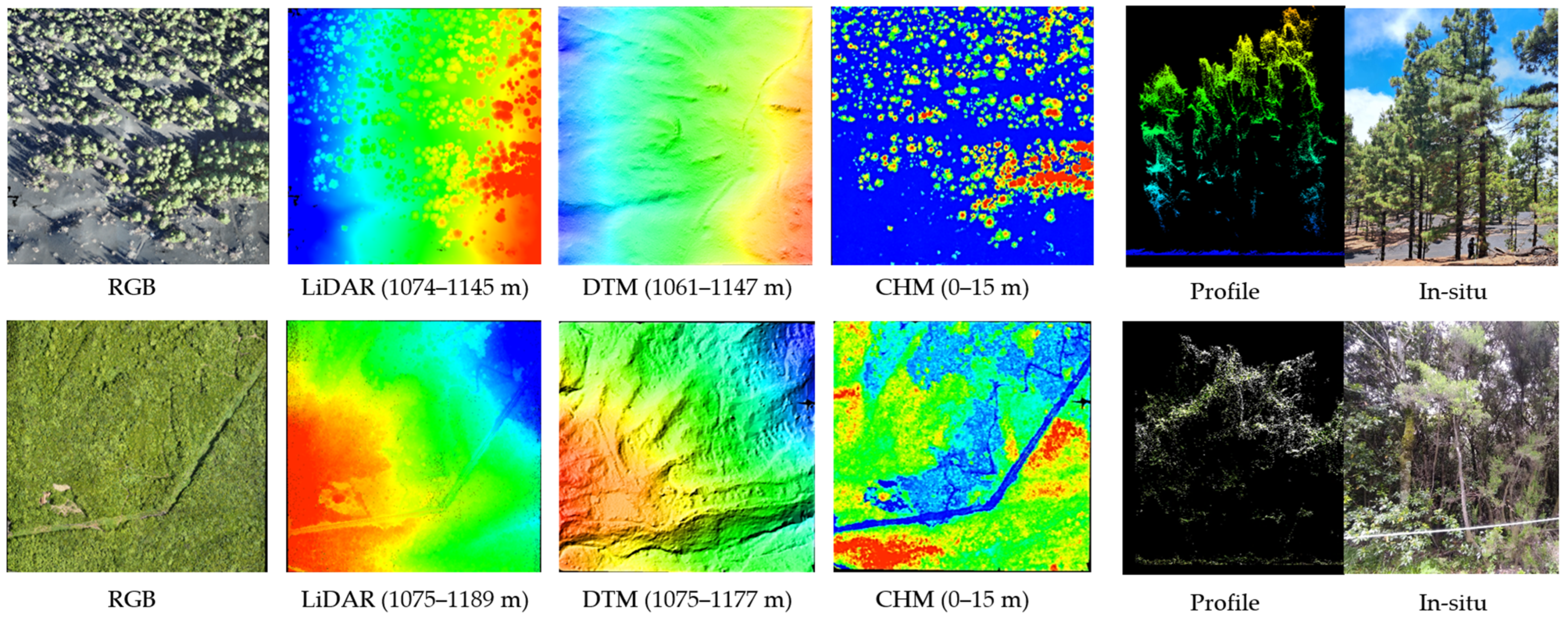
For the generation of the DTM, several approaches based on spatial interpolation of ground-classified points can be applied to estimate terrain elevations in unsampled areas. After evaluating three main interpolation techniques (Kriging, Inverse Distance Weighting, and TIN-based interpolation) [55,56], the TIN-based method again provided the best results. Subsequently, the DSM was generated from the highest LiDAR returns representing the upper surface of the vegetation. The CHM was then calculated by subtracting the DTM from the DSM, providing the vegetation height above the local ground surface. The following figure illustrates the three derived models. Figure A2 illustrates an example of LiDAR-derived products for two plots characterized by contrasting vegetation types: one located in a pine forest area and the other dominated by dense fayal-brezal vegetation. The figure includes the true-color RGB image, the original LiDAR point-cloud raster, in which elevations are represented using a rainbow color palette ranging from blue (lower values) to red (higher values), as well as the corresponding Digital Terrain Model and Canopy Height Model. Finally, the figure also displays a vertical profile extracted from the LiDAR data together with a field photograph taken at the same location during the ground survey.
Figure A2. RGB and LiDAR data acquired with the Zenmuse sensor over plots 5 (upper row) and 39 (lower row). Blue colors represent the lower elevation or height values, while reddish colors the higher values.
Remotesensing 18 02871 g0a2
For the classification stage, a properly parametrized Support Vector Machine algorithm using a Radial Basis Function kernel was employed [57], owing to its robustness and its capability to deliver high classification accuracy even when training data are limited. Classified maps were generated using different combinations of input features derived from the available UAV data, including multispectral and LiDAR products. As expected, the best results were obtained by combining multispectral bands with the CHM and DTMs. For each UAV plot, classification accuracy was assessed using validation ROIs that were spatially independent from those used to train the SVM classifier. Table A1 summarizes the accuracy results obtained for all plots, showing that an overall accuracy over 98% was achieved on average. In Section 3.2 (Figure 7) an example was presented covering two plots characterized by different types of forest vegetation (plot 19: pines + shrubs, and plot 41: laurisilva + fayal-brezal + chestnuts).
Table A1. Accuracy of the SVM classifier for all the plots sampled.
Plot NumberAccuracy (%)Kappa
LF-BPCOVS&OGlobal
1 97.13 98.9799.5997.980.9639
298.4999.38 76.2110098.390.9267
3 99.56 86.6110098.610.9753
4 97.72 80.6897.8696.190.9205
5 99.54 99.3899.9999.680.9947
6 98.92 99.4299.450.9834
7 93.89 88.3699.5395.120.9234
8 96.11 83.5999.8895.190.8930
9 99.53 95.0398.870.9544
10 98.52 53.7199.2696.650.9379
11 80.41 94.4199.8887.140.7868
12 99.83 95.4599.9099.610.9926
13 99.01 98.0899.1898.880.9822
14 95.60 88.4098.0395.630.9165
15 99.83 99.6210099.820.9965
16 98.36 99.0698.640.9716
1799.88 10099.890.9639
1899.2092.67 93.78 88.9397.260.9349
19 97.08 98.8694.5897.320.9559
20 97.80 97.4699.3298.050.9644
21 99.40 97.8895.3898.370.9686
22 99.7699.71 99.3599.720.9946
23 99.27 99.1099.6299.350.9893
2485.3093.02 79.7499.5590.480.8055
25 99.12 98.3499.120.6913
26 99.59 98.2999.9599.550.9925
27 98.43 92.5399.9196.410.9434
28 94.61 99.9899.9698.630.9788
2999.88 99.2799.7599.770.9931
30 99.7994.18 99.9995.790.9063
3199.8599.06 94.9295.2398.610.9729
32 97.44 99.78 98.060.9512
33 99.37 93.7597.8998.350.9634
34 99.85 96.3699.5999.360.9823
35 99.97 10099.980.9996
3699.98 96.5399.9699.9299.960.9992
37 97.95 98.4098.2598.060.9569
38 98.86 96.8484.2195.960.9246
39 99.84 98.5599.4499.730.9894
4091.9299.13 95.51 94.100.8874
4194.9092.82 89.16 96.9894.100.8754
42 99.61 97.0498.9798.980.9830
43 99.80 99.8899.850.9969
L: Laurisilva, F-B: Fayal-Brezal, P: Pine, C: Chestnut, OV: Other Vegetation, S&O: Soil & Others.

References

  1. Cabildo de La Palma. Medio Ambiente—Cabildo de La Palma. Available online: https://www.cabildodelapalma.es/es/medioambiente (accessed on 25 January 2026).
  2. Weiser, F.; Baumann, E.; Jentsch, A.; Medina, F.M.; Lu, M.; Nogales, M.; Beierkuhnlein, C. Impact of Volcanic Sulfur Emissions on the Pine Forest of La Palma, Spain. Forests 2022, 13, 299. [Google Scholar] [CrossRef] [Scilit]
  3. Vantor/Maxar. Our Constellation. Available online: https://maxarenergysource.com/maxar-intelligence/constellation.html (accessed on 25 January 2026).
  4. Zhong, L.; Dai, Z.; Fang, P.; Cao, Y.; Wang, L. A Review: Tree Species Classification Based on Remote Sensing Data and Classic Deep Learning-Based Methods. Forests 2024, 15, 852. [Google Scholar] [CrossRef] [Scilit]
  5. Sheykhmousa, M.; Mahdianpari, M.; Ghanbari, H.; Mohammadimanesh, F.; Ghamisi, P.; Homayouni, S. Support Vector Machine versus Random Forest for Remote Sensing Image Classification: A Meta-Analysis and Systematic Review. IEEE J. Sel. Top. Appl. Earth Obs. Remote Sens. 2020, 13, 6308–6325. [Google Scholar] [CrossRef] [Scilit]
  6. Fassnacht, F.E.; Latifi, H.; Stereńczak, K.; Modzelewska, A.; Lefsky, M.; Waser, L.T.; Straub, C.; Ghosh, A. Review of Studies on Tree Species Classification from Remote Sensed Data. Remote Sens. Environ. 2016, 186, 64–87. [Google Scholar] [CrossRef] [Scilit]
  7. Boston, T.; Van Dijk, A.; Rozas Larraondo, P.; Thackway, R. Comparing CNNs and Random Forests for Landsat Image Segmentation Trained on a Large Proxy Land Cover Dataset. Remote Sens. 2022, 14, 3396. [Google Scholar] [CrossRef] [Scilit]
  8. Aziz, G.; Minallah, N.; Saeed, A.; Frnda, J.; Khan, W. Remote Sensing-Based Forest Cover Classification Using Machine Learning. Sci. Rep. 2024, 14, 69. [Google Scholar] [CrossRef] [Scilit]
  9. Kattenborn, T.; Leitloff, J.; Schiefer, F.; Hinz, S. Review on Convolutional Neural Networks (CNN) in Vegetation Remote Sensing. ISPRS J. Photogramm. Remote Sens. 2021, 173, 24–49. [Google Scholar] [CrossRef] [Scilit]
  10. Ayhan, B.; Kwan, C.; Budavári, B.; Kwan, L.; Lu, Y.; Perez, D.; Li, J.; Skarlatos, D.; Vlachos, M. Vegetation Detection Using Deep Learning and Conventional Methods. Remote Sens. 2020, 12, 2502. [Google Scholar] [CrossRef] [Scilit]
  11. Boston, T.; Van Dijk, A.; Thackway, R. U-Net Convolutional Neural Network for Mapping Natural Vegetation and Forest Types from Landsat Imagery in Southeastern Australia. J. Imaging 2024, 10, 143. [Google Scholar] [CrossRef] [Scilit]
  12. Chen, S.; Zhang, M.; Lei, F. Mapping Vegetation Types by Different Fully Convolutional Neural Network Structures with Inadequate Training Labels in Complex Landscape Urban Areas. Forests 2023, 14, 1788. [Google Scholar] [CrossRef] [Scilit]
  13. Cao, Q.; Li, M.; Yang, G.; Tao, Q.; Luo, Y.; Wang, R.; Chen, P. Urban Vegetation Classification for UAV Remote Sensing Combining Feature Engineering and Improved DeepLabV3+. Forests 2024, 15, 382. [Google Scholar] [CrossRef] [Scilit]
  14. Drobnjak, S.; Stojanović, M.; Djordjević, D.; Bakrač, S.; Jovanović, J.; Djordjević, A. Testing a New Ensemble Vegetation Classification Method Based on Deep Learning and Machine Learning Using Aerial Photogrammetric Images. Front. Environ. Sci. 2022, 10, 896158. [Google Scholar] [CrossRef] [Scilit]
  15. Bazi, Y.; Bashmal, L.; Al Rahhal, M.M.; Dayil, R.A.; Ajlan, N.A. Vision Transformers for Remote Sensing Image Classification. Remote Sens. 2021, 13, 516. [Google Scholar] [CrossRef] [Scilit]
  16. Xie, E.; Wang, W.; Yu, Z.; Anandkumar, A.; Alvarez, J.M.; Luo, P. SegFormer: Simple and Efficient Design for Semantic Segmentation with Transformers. Adv. Neural Inf. Process. Syst. 2021, 34, 12077–12090. [Google Scholar]
  17. Li, M.; Rui, J.; Yang, S.; Liu, Z.; Ren, L.; Ma, L.; Li, Q.; Su, X.; Zuo, X. Method of Building Detection in Optical Remote Sensing Images Based on SegFormer. Sensors 2023, 23, 1258. [Google Scholar] [CrossRef] [Scilit]
  18. Sertel, E.; Hucko, C.M.; Kabadayı, M.E. Automatic Road Extraction from Historical Maps Using Transformer-Based SegFormers. ISPRS Int. J. Geo-Inf. 2024, 13, 464. [Google Scholar] [CrossRef] [Scilit]
  19. Wang, X.; Chen, S.; Yan, H.; Yang, H.; Yan, Z.; Wang, S. Road Recognition in Remote Sensing Images Using SegFormer Fused with Attention Mechanism. Comput. Syst. Appl. 2024, 33, 186–193. [Google Scholar]
  20. Yang, L.; Wang, X.; Zhai, J. Waterline Extraction for Artificial Coast with Vision Transformers. Front. Environ. Sci. 2022, 10, 799250. [Google Scholar] [CrossRef] [Scilit]
  21. Drakopoulou, P.; Tzouveli, P.; Karditsa, A.; Poulos, S. Integrating AI for In-Depth Segmentation of Coastal Environments in Remote Sensing Imagery. Remote Sens. 2026, 18, 325. [Google Scholar] [CrossRef] [Scilit]
  22. Chen, Y.; Wang, X. Farmland Extraction from UAV Remote Sensing Images Based on Improved SegFormer Model. J. Indian Soc. Remote Sens. 2025, 53, 421–433. [Google Scholar] [CrossRef] [Scilit]
  23. Wu, Y.; Tang, L.; Yuan, S. Semantic Segmentation Model of Multi-Source Remote Sensing Images Was Used to Extract Winter Wheat at Tillering Stage (Tif-SegFormer). Sci. Rep. 2025, 15, 98449. [Google Scholar] [CrossRef] [Scilit]
  24. Xie, J.; Hua, J.; Chen, S.; Wu, P.; Gao, P.; Sun, D.; Lyu, Z.; Lyu, S.; Xue, X.; Lu, J. HyperSFormer: A Transformer-Based End-to-End Hyperspectral Image Classification Method for Crop Classification. Remote Sens. 2023, 15, 3491. [Google Scholar] [CrossRef] [Scilit]
  25. Phahurat, S.; Thongsang, P.; Chotpantarat, S. CropNet: Leveraging SegFormer for Efficient and Scalable Crop Mapping with Sentinel-2 Data. Bull. Earth Sci. Thail. 2025, 17, 36–49. [Google Scholar]
  26. Dong, M.; Cao, H.; Zhao, T.; Zhao, X. SegFormer-Based Nectar Source Segmentation in Remote Sensing Imagery. Front. Plant Sci. 2025, 16, 1666619. [Google Scholar] [CrossRef] [Scilit]
  27. Spasev, V.; Dimitrovski, I.; Chorbev, I.; Kitanovski, I. Semantic Segmentation of Unmanned Aerial Vehicle Remote Sensing Images using SegFormer. arXiv 2024, arXiv:2410.01092. [Google Scholar] [CrossRef] [Scilit]
  28. Infraestructura de Datos Espaciales de Canarias (IDECanarias). Actualización del Mapa de Vegetación de Canarias en las Islas de La Palma y Lanzarote—Memoria Final (2021-C06) Diciembre 2021; 52 pp. PDF Disponible en. Available online: https://www.idecanarias.es/resources/Vegetacion/2021/2021_C06_memoria_idecanarias.pdf (accessed on 25 January 2026).
  29. Devkota, R.S.; Field, R.; Hoffmann, S.; Walentowitz, A.; Medina, F.M.; Vetaas, O.R.; Chiarucci, A.; Weiser, F.; Jentsch, A.; Beierkuhnlein, C. Assessing the Potential Replacement of Laurel Forest by a Novel Ecosystem in the Steep Terrain of an Oceanic Island. Remote Sens. 2020, 12, 4013. [Google Scholar] [CrossRef] [Scilit]
  30. Instituto Geográfico Nacional (CNIG). Modelos Digitales de Elevaciones—Centro de Descargas. Available online: https://centrodedescargas.cnig.es/CentroDescargas/modelos-digitales-elevaciones (accessed on 25 January 2026).
  31. Luque Söllheim, Á.L.; Máyer Suárez, P.; García Hernández, F. The Digital Climate Atlas of the Canary Islands: A Tool to Improve Knowledge of Climate and Temperature and Precipitation Trends in the Atlantic Islands. Clim. Serv. 2024, 34, 100487. [Google Scholar] [CrossRef] [Scilit]
  32. Marcello, J.; Eugenio, F.; Perdomo, U.; Medina, A. Assessment of Atmospheric Algorithms to Retrieve Vegetation in Natural Protected Areas Using Multispectral High Resolution Imagery. Sensors 2016, 16, 1624. [Google Scholar] [CrossRef] [Scilit]
  33. Marcello, J.; Eugenio, F.; Gonzalo-Martín, C.; Rodríguez-Esparragón, D.; Marqués, F. Advanced Processing of Multiplatform Remote Sensing Imagery for the Monitoring of Coastal and Mountain Ecosystems. IEEE Access 2021, 9, 6536–6549. [Google Scholar] [CrossRef] [Scilit]
  34. Anderson, G.P.; Felde, G.W.; Hoke, M.L.; Ratkowski, A.J.; Cooley, T.W.; Chetwynd, J.H., Jr.; Gardner, J.A.; Adler-Golden, S.M.; Matthew, M.W.; Berk, A.; et al. MODTRAN4-Based Atmospheric Correction Algorithm: FLAASH (Fast Line-of-Sight Atmospheric Analysis of Spectral Hypercubes). In Proceedings of the SPIE: Algorithms and Technologies for Multispectral, Hyperspectral, and Ultraspectral Imagery VIII, Orlando, FL, USA, 1–4 April 2002; SPIE: Bellingham, WA, USA, 2002; p. 4725. [Google Scholar] [CrossRef] [Scilit]
  35. NASA GES DISC. Giovanni—The Bridge Between Data and Science. Available online: https://giovanni.gsfc.nasa.gov/giovanni/ (accessed on 25 January 2026).
  36. NASA MODIS Atmosphere Team. Aerosol (MOD04/MYD04) Product—Dark Target & Deep Blue Algorithms. Available online: https://atmosphere-imager.gsfc.nasa.gov/products/aerosol (accessed on 25 January 2026).
  37. Rodríguez-Esparragón, D.; Marcello, J.; Eugenio, F.; Gamba, P. Index-Based Forest Degradation Mapping Using High and Medium Resolution Multispectral Sensors. Int. J. Digit. Earth 2024, 17, 2365981. [Google Scholar] [CrossRef] [Scilit]
  38. Richards, J.A. Remote Sensing Digital Image Analysis; Springer: Cham, Switzerland, 2022. [Google Scholar] [CrossRef] [Scilit]
  39. Medina Machín, A.; Marcello, J.; Hernández-Cordero, A.I.; Martín Abasolo, J.; Eugenio, F. Vegetation Species Mapping in a Coastal Dune Ecosystem Using High Resolution Satellite Imagery. GISci. Remote Sens. 2019, 56, 210–232. [Google Scholar] [CrossRef] [Scilit]
  40. Marcello, J.; Spínola, M.; Albors, L.; Marqués, F.; Rodríguez-Esparragón, D.; Eugenio, F. Performance of Individual Tree Segmentation Algorithms in Forest Ecosystems Using UAV LiDAR Data. Drones 2024, 8, 772. [Google Scholar] [CrossRef] [Scilit]
  41. Rodríguez-Dorna, A.; Alonso, L.; Costas, F.; Picos, J.; Armesto, J. Very High Resolution WorldView-3 Images for Land Cover Mapping on a Large Scale: Strengths and Remaining Challenges. Geocarto Int. 2025, 40, 2538802. [Google Scholar] [CrossRef] [Scilit]
  42. Immitzer, M.; Atzberger, C.; Koukal, T. Tree Species Classification with Random Forest Using Very High Spatial Resolution 8-Band WorldView-2 Satellite Data. Remote Sens. 2012, 4, 2661–2693. [Google Scholar] [CrossRef] [Scilit]
  43. Prodromou, M.; Theocharidis, C.; Gitas, I.Z.; Eliades, F.; Themistocleous, K.; Papasavvas, K.; Dimitrakopoulos, C.; Danezis, C.; Hadjimitsis, D. Forest Habitat Mapping in Natura2000 Regions in Cyprus Using Sentinel-1, Sentinel-2 and Topographical Features. Remote Sens. 2024, 16, 1373. [Google Scholar] [CrossRef] [Scilit]
  44. Thanh Noi, P.; Kappas, M. Comparison of Random Forest, k-Nearest Neighbor, and Support Vector Machine Classifiers for Land Cover Classification Using Sentinel-2 Imagery. Sensors 2018, 18, 18. [Google Scholar] [CrossRef] [Scilit]
  45. Adugna, T.; Xu, W.; Fan, J. Comparison of Random Forest and Support Vector Machine Classifiers for Regional Land Cover Mapping Using Coarse Resolution FY-3C Images. Remote Sens. 2022, 14, 574. [Google Scholar] [CrossRef] [Scilit]
  46. Ouma, Y.; Nkwae, B.; Moalafhi, D.; Odirile, P.; Parida, B.; Anderson, G.; Qi, J. Comparison of Machine Learning Classifiers for Multi-Temporal and Multi-Sensor Urban LULC Mapping. Int. Arch. Photogramm. Remote Sens. Spat. Inf. Sci. 2022, 43, 681–689. [Google Scholar] [CrossRef] [Scilit]
  47. Belgiu, M.; Drăguţ, L. Random Forest in Remote Sensing: A Review of Applications and Future Directions. ISPRS J. Photogramm. Remote Sens. 2016, 114, 24–31. [Google Scholar] [CrossRef] [Scilit]
  48. Zhao, W.; Du, S.; Emery, W.J. A Comparative Analysis of Convolutional Neural Networks and Vision Transformers for Remote Sensing Image Segmentation. Remote Sens. 2022, 14, 3286. [Google Scholar] [CrossRef] [Scilit]
  49. Li, Y.; Zhang, H.; Shen, Q.; Wang, S. On the Limitations of Vision Transformers in Remote Sensing Image Classification with Limited Training Data. IEEE Geosci. Remote Sens. Lett. 2023, 20, 1–5. [Google Scholar]
  50. Guidici, D.; Clark, M.L. One-Dimensional Convolutional Neural Network Land-Cover Classification of Multi-Seasonal Hyperspectral Imagery in the San Francisco Bay Area, California. Remote Sens. 2017, 9, 629. [Google Scholar] [CrossRef] [Scilit]
  51. Rodríguez Paulino, E.; Schlerf, M.; Röder, A.; Stoffels, J.; Udelhoven, T. Forest disturbance characterization in the era of earth observation big data: A mapping review. Int. J. Appl. Earth Obs. Geoinf. 2024, 128, 103755. [Google Scholar] [CrossRef] [Scilit]
  52. Zhang, K.; Chen, S.C.; Whitman, D.; Shyu, M.L.; Yan, J.; Zhang, C. A progressive morphological filter for removing nonground measurements from airborne LIDAR data. IEEE Trans. Geosci. Remote Sens. 2003, 41, 872–882. [Google Scholar] [CrossRef] [Scilit]
  53. Zhang, W.; Qi, J.; Wan, P.; Wang, H.; Xie, D.; Wang, X.; Yan, G. An Easy-to-Use Airborne LiDAR Data Filtering Method Based on Cloth Simulation. Remote Sens. 2016, 8, 501. [Google Scholar] [CrossRef] [Scilit]
  54. Chen, N.; Wang, N.; He, Y.; Ding, X.; Kong, J. An improved progressive triangular irregular network densification filtering algorithm for airborne LiDAR data. Front Earth Sci. 2023, 10, 1015153. [Google Scholar] [CrossRef] [Scilit]
  55. Lu, G.Y.; Wong, D.W. An adaptive inverse-distance weighting spatial interpolation technique. Comput. Geosci. 2008, 34, 1044–1055. [Google Scholar] [CrossRef] [Scilit]
  56. Lloyd, C.D.; Atkinson, P.M. Deriving DSMs from LiDAR data with kriging. Int. J. Remote Sens. 2002, 23, 2519–2524. [Google Scholar] [CrossRef] [Scilit]
  57. Mansor, N.S.; Awang, H.; Shehu Malami, S.T.; Zolkafli, A.; Taiye, M.A.; Maulana, H. Support Vector Machine for Satellite Images Classification Using Radial Basis Function Kernel Method. In Computing and Informatics (ICOCI 2023); Springer: Singapore, 2024; pp. 301–312. [Google Scholar] [CrossRef] [Scilit]
Figure 1. Location of La Palma island (GRAFCAN, orthophoto 5 October 2023) and its main forest ecosystems.
Remotesensing 18 02871 g001
Figure 2. Preprocessing of WorldView imagery: (a) Spatial extent and delineation of the scenes employed in the analysis, (b) individual WorldView acquisitions, (c) WorldView scenes, and (d) final WorldView composite after corrections and mosaicking the scenes.
Remotesensing 18 02871 g002
Figure 3. Data: (a) WorldView-2 image from 4 May 2024, (b) surveyed UAV plots (yellow boxes), (c) map with the most representative forest types (Canary Islands Government, 2021), (d) digital terrain model (m), (e) slope (°), (f) aspect (0°: N, 90°: E, 180°: S, 270°: W), (g) annual accumulated precipitation 1975–2020 (mm), and (h) mean annual temperature (°C).
Remotesensing 18 02871 g003
Figure 4. Overall workflow for data preprocessing, evaluation of the classification algorithms, and production of the final forest vegetation map.
Remotesensing 18 02871 g004
Figure 5. Spectral signatures for a vegetation pixel (red bullet) at different processing stages: (a) original digital numbers, (b) radiometrically calibrated radiance, and (c) atmospherically corrected reflectance (×10,000 factor included).
Remotesensing 18 02871 g005
Figure 6. Spatial differences observed in two areas before and after orthorectification and geolocation correction. Transparency overlays highlight geometric misalignments prior to corrections.
Remotesensing 18 02871 g006
Figure 7. Classification results for plots 19 and 41: (a) multispectral data, (b) DTM, (c) CHM, and (d) SVM classification map.
Remotesensing 18 02871 g007
Figure 8. Mapping of forest vegetation on La Palma for the classifiers analyzed using spectral, textural and topographical information.
Remotesensing 18 02871 g008
Figure 9. Forest vegetation mapping of La Palma using all the relevant features (MS + WDRVI + Texture + DTM + Slope + Aspect) for the remote sensing derived maps: (a) Government of the Canary Islands map (2021), (b) Random Forest, and (c) SegFormer.
Remotesensing 18 02871 g009
Figure 10. Time series of vegetation index derived from cloud-free Sentinel-2 imagery at habitat level. The dashed lines represent the linear trends.
Remotesensing 18 02871 g010
Figure 11. Topography of La Palma island: (a) orthophoto, (b) digital terrain model and (c) topographic profile of an area crossing the Caldera de Taburiente (yellow line overlaid on the orthophoto).
Remotesensing 18 02871 g011
Figure 12. Shrub species of La Palma: (a) tabaibas (Euphorbia balsamifera), (b) cardones (Euphorbia canariensis), and (c) jarales (Cistus monspeliensis).
Remotesensing 18 02871 g012
Table 1. Spectral and spatial specifications of the WorldView-2/3 and MicaSense RedEdge-MX Dual multispectral datasets.
Platform/SensorWorldView-2/WorldView-3UAV MicaSense
Spectral Bands and
Center Wavelength
(nm)
Coastal
Blue
Green
Yellow
Red
Red Edge
NIR1
NIR2
427
478
546
608
659
724
831
908
Coastal Blue
Blue
Green
Green
Red
Red
Red Edge
Red Edge
Red Edge
NIR
444
475
531
560
650
668
705
717
740
842
Native spatial resolutionWV-2: 1.84 m at nadir
WV-3: 1.24 m at nadir
8 cm/pixel at 120 m
(depends on flight altitude)
Spatial resolution used2.0 m10 cm
Table 2. Information on the WorldView scenes used to generate the composite image of La Palma.
ParametersScene 1Scene 2Scene 3Scene 4
Satellite: WV03WV03WV03 WV02
Date: 4 May 20244 May 202413 July 202412 August 2024
ID: 1040010093963A0010400100956C7A00104001009790D5001030010102C39200
Cloud percentage: 0.0%0.0%3.0%0.0%
Off Nadir:27.7°28.5°23.5°10°
GSD (PAN band): 0.38 m0.40 m0.37 m0.48 m
Sun Elevation: 71.4°71.5°72.3°66.3°
Max Target Azimuth: 91.2°117.3°84.6°234.4°
Table 3. Spectral separability, expressed as Jeffries–Matusita (JM) distance, across the WorldView spectral bands for each pair of classes, ordered from lowest to highest value.
Training ROIsTesting ROIs
0.721: Laurisilva-Fayal-Brezal 0.326: Laurisilva-Fayal-Brezal
1.282: Other_vegetation-Pine 1.283: Other_vegetation-Pine
1.338: Other_vegetation-Chestnut 1.401: Fayal-Brezal-Pine
1.627: Fayal-Brezal-Pine1.417: Other_vegetation-Chestnut
1.666: Other_vegetation-Fayal-Brezal1.571: Laurisilva-Pine
1.743: Laurisilva-Pine1.719: Other_vegetation-Fayal-Brezal
1.771: Fayal-Brezal-Chestnut1.764: Other_vegetation-Laurisilva
1.823: Other_vegetation-Laurisilva1.801: Fayal-Brezal-Chestnut
1.829: Soil/Others-Other_vegetation1.830: Laurisilva-Chestnut
1.846: Pine-Chestnut1.843: Pine-Chestnut
1.908: Laurisilva-Chestnut1.961: Soil/Others-Other_vegetation
1.931: Soil/Others–Pine1.987: Soil/Others–Pine
1.963: Soil/Others-Chestnut1.989: Soil/Others-Chestnut
1.988: Soil/Others-Fayal-Brezal1.996: Soil/Others–Laurisilva
1.993: Soil/Others-Laurisilva1.996: Soil/Others-Fayal-Brezal
Table 4. Classification accuracy achieved by the nine classifiers using two input data combinations.
Algorithm **InputUser’s Accuracy (%)Kappa
LF-BPCOVS&OOA
MDMS55.225.932.044.326.957.540.10.280
All *56.225.532.282.412.055.043.10.317
MhDMS60.731.447.072.254.079.057.20.485
All57.233.948.776.120.272.150.50.407
PMS20.35.129.60.039.249.524.20.130
All16.824.819.614.132.98.8718.90.140
SAM MS55.934.711.374.617.178.944.60.335
All58.833.133.792.23.175.348.10.378
MLMS71.942.067.992.062.987.270.40.645
All66.552.670.492.580.485.274.50.694
NBMS53.246.824.977.554.186.956.80.482
All47.470.247.184.173.679.566.60.600
KNNMS63.547.465.486.858.599.469.50.634
All60.848.174.486.180.697.674.40.692
RFMS72.849.575.891.570.399.076.10.713
All75.744.279.889.678.498.377.50.730
SVMMS73.749.571.189.365.098.374.10.689
All70.047.170.991.268.497.673.80.685
* All: MS + WDRVI + Texture + DTM + Slope + Aspect; ** MD: Minimum Distance, MhD: Mahalanobis Distance, P: Parallelepiped, SAM: Spectral Angle Mapper, ML: Maximum Likelihood, NB: Naïve Bayes, KNN: K-Nearest Neighbors, RF: Random Forest, SVM: Support Vector Machine. Bold values indicate the two best accuracy results in each column. The shaded row indicates the best-performing classification algorithm.
Table 5. Accuracy of the Random Forest classifier using different input data combinations.
Input *User’s Accuracy (%)Kappa
LF-BPCOVS&OOA
MS72.849.575.891.570.399.076.10.713
MS + WDRVI72.649.476.091.569.999.476.10.713
MS + Text71.349.676.282.565.168.968.90.633
MS + DTM71.242.778.990.478.498.376.50.717
MS + Slope75.551.077.589.965.798.575.90.711
MS + Aspect74.449.775.290.574.198.976.80.722
MS + Precipitation56.744.969.593.763.090.569.10.631
MS + Temperature62.942.770.084.575.090.470.70.649
MS + VI + S + A76.451.778.489.266.398.676.30.716
MS + VI + S + A + P + T57.847.676.286.260.595.469.90.640
MS + VI + Tx + DTM + S + A75.744.279.889.678.398.377.50.730
MS + VI + Tx + DTM + S + A + P + T62.948.478.893.465.196.673.60.684
* VI: WDRVI, Tx: Texture, S: Slope, A: Aspect, P: Precipitation, T: Temperature.
Table 6. Accuracy of the SegFormer classifier using two input data combinations.
AlgorithmInputUser’s Accuracy (%)Kappa
LF-BPCOVS&OOA
SegFormerMS52.340.758.147.623.662.658.10.40
All77.462.384.687.584.684.775.50.64
Disclaimer/Publisher’s Note: The statements, opinions and data contained in all publications are solely those of the individual author(s) and contributor(s) and not of MDPI and/or the editor(s). MDPI and/or the editor(s) disclaim responsibility for any injury to people or property resulting from any ideas, methods, instructions or products referred to in the content.