SAR-Oriented and Physics-Guided Ocean Wave Spectrum Retrieval

Highlights

What are the main findings?

• We developed PGT-Swin, a physics-guided, texture-enhanced Swin Transformer for retrieving ocean wave spectra from SAR images.
• PGT-Swin improves wave-spectrum reconstruction and provides reliable estimates of significant wave height (SWH) and mean wave period (MWP).

What are the implications of the main findings?

• Compared with direct regression of scalar wave parameters, the retrieved spectra provide more physically consistent information for preliminary wave-energy characterization.
• The framework supports large-scale ocean-wave monitoring using SAR imagery and may improve the reliability of preliminary wave-energy characterization.

Abstract

Accurate retrieval of ocean wave spectra from Synthetic Aperture Radar (SAR) images is important for understanding wave energy distribution and supporting large-scale ocean-wave monitoring. However, existing SAR-based wave retrieval methods often focus on scalar wave parameters and pay limited attention to the physical consistency of spectral energy reconstruction. In this study, we propose a physics-guided texture-enhanced Swin Transformer, named PGT-Swin, for retrieving one-dimensional wave frequency spectra from SAR images. The proposed method first constructs multi-channel SAR representations by combining intensity-enhanced images with Gray-Level Co-Occurrence Matrix (GLCM)-based texture features. A Swin Transformer backbone is then used to capture both local wave textures and global periodic structures. In addition, physics-guided spectral constraints are introduced to preserve total spectral energy and frequency-distribution consistency. Experiments were conducted using collocated Sentinel-1 SAR images and one-dimensional frequency spectra derived from CFOSAT SWIM products. The results show that PGT-Swin can effectively reconstruct wave spectra and derive reliable integral wave parameters. For SWH retrieval, the model achieves an MSE of 0.0014 and an R² of 0.9591. For MWP retrieval, it achieves an MSE of 0.0295 and an R² of 0.6659. These results demonstrate the effectiveness of PGT-Swin for SAR-based one-dimensional wave frequency-spectrum retrieval within the evaluated SWIM-referenced setting.

1. Introduction

Wave energy has emerged as one of the most promising renewable energy sources due to its vast potential, predictability, and low environmental impact [1,2]. The effective utilization of wave energy not only contributes to sustainable electricity generation but also supports coastal and offshore infrastructure planning [3]. Among various aspects of wave energy, the energy contained in ocean waves plays a critical role, as it directly reflects the transport and distribution of kinetic and potential energy across the sea surface. The accurate quantification of wave energy is, therefore, essential for evaluating marine energy resources, supporting offshore engineering design, and enabling large-scale ocean energy monitoring [4]. In this context, the ocean wave frequency spectrum plays a fundamental role, as it provides a complete description of the energy distribution across different frequencies, and serves as the basis for deriving key integral wave parameters, such as significant wave height (SWH) and mean wave period (MWP).

Accurate wave parameters are essential for ocean energy development, coastal engineering, and climate change research [5,6,7,8,9]. Traditional wave observations are mainly obtained from in situ instruments, such as buoys and ship-borne measurements. Although these observations can provide accurate local wave information, they are limited by sparse spatial coverage, high deployment and maintenance costs, and discontinuous temporal sampling. These limitations make it difficult to support real-time and large-scale monitoring of ocean wave energy [10,11]. With the rapid development of satellite remote sensing, Synthetic aperture radar (SAR) is well suited to ocean wave observation because it provides wide-swath, high-resolution measurements of the sea surface under all weather conditions and without direct contact [12,13,14]. Therefore, SAR imagery provides a promising data source for large-scale wave spectrum retrieval and preliminary wave-energy characterization.

However, retrieving wave spectra from SAR imagery remains a challenging inverse problem. The SAR imaging process of ocean waves is governed by a complex nonlinear mapping between the sea surface wave field and the SAR image intensity. This mapping is affected by multiple physical modulation mechanisms, including tilt modulation, hydrodynamic modulation, and velocity bunching effects [15,16]. In addition, speckle noise, imaging distortions, changing sea states, wind-wave interactions, and nonlinear wave conditions further increase the uncertainty of SAR-based wave retrieval. Although bulk wave parameters, such as SWH and MWP, are widely available from satellites, buoys, and numerical models, frequency-resolved observations have much sparser spatial and temporal coverage [17]. This matters because SWH and MWP summarize the spectrum through integral quantities. Different spectra can yield similar values of SWH and MWP while differing in peak frequency, bandwidth, secondary peaks, and the distribution of energy among frequency bands [18]. Agreement in these bulk parameters, therefore, does not ensure that the underlying spectral structure or its evolution is represented correctly. This gap constrains applications that depend on spectral shape. Validation based only on SWH and MWP can miss errors in a wave model’s peak frequency, bandwidth, or high-frequency energy [19]. Spectral observations are also needed to study wave growth, propagation, dissipation, and energy transfer across frequencies. A one-dimensional spectrum may distinguish wind–sea and swell components when their peaks occupy different frequency bands, but it cannot separate systems that overlap in frequency and propagate in different directions. Such cases require directional spectra.

In this study, we propose a deep learning framework based on the Swin Transformer to retrieve one-dimensional wave frequency spectra from SAR images and subsequently derive SWH and MWP through spectral integration. The proposed method uses the hierarchical structure and shifted-window attention mechanism of the Swin Transformer to capture both global energy patterns and local energy variations in remote sensing images. We regard wave parameter retrieval as a feature extraction task based on the energy-related patterns contained in the images. In this way, the proposed model builds a connection between image features and physical oceanographic parameters and provides an accurate and efficient solution for large-scale ocean energy monitoring. In a nutshell, the contributions of our work are summarized as follows:

• We propose a wave spectrum retrieval framework named PGT-Swin, which directly predicts frequency-resolved one-dimensional wave spectra from SAR images.
• PGT-Swin designs a multi-channel feature enhancement strategy to integrate intensity information and texture-aware representations for improved wave feature characterization.
• PGT-Swin enhances the physical consistency of wave spectrum retrieval through physically guided wave spectrum constraints.
• Extensive experiments demonstrate the effectiveness of PGT-Swin in reconstructing frequency spectra and deriving SWH and MWP estimates.

Finally, experimental results show that the proposed method achieves accurate wave spectrum retrieval, with $R^2$ values of 0.9591 and 0.6659 for the derived SWH and MWP, respectively. The proposed framework uses collocated SAR and SWIM observations to learn a mapping from SAR image features to SWIM-referenced one-dimensional frequency spectra. Once trained, it requires only a SAR image and may, therefore, provide spectral estimates when no concurrent SWIM observation is available. The method is intended not to replace SWIM products but to extend the spectral information learned from collocated observations to SAR-only acquisitions. Subject to the uncertainties associated with this cross-sensor mapping, these estimates could support spectrum-level model evaluation, studies of spectral variability, and marine applications that depend on the frequency distribution of wave energy.

2. Literature Review

In this section, we review some related works, including inversion of ocean parameters and deep learning in remote sensing.

2.1. Inversion of Ocean Parameters Based on SAR

The theoretical foundation of retrieving ocean wave parameters from SAR imagery lies in understanding the complex, non-linear mapping mechanism between the ocean surface and the SAR image intensity [20,21]. This mapping is primarily governed by tilt modulation [22], hydrodynamic modulation [23], and velocity bunching effects [24]. Classical physical inversion schemes, such as the Max-Planck Institute (MPI) algorithm and the Semi-Parametric Retrieval Algorithm (SPRA), rely on the nonlinear integral transform relation described by Hasselmann [25,26,27]. While these methods are physically rigorous, they are computationally intensive and inherently ill-posed, often requiring a high-precision “first-guess spectrum”, which usually come from numerical wave models like WAM or WW3 to resolve the ambiguity [28,29]. This heavy reliance on external prior information limits their applicability in stand-alone inversion scenarios.

To bypass the complexity of physical modulation transfer functions (MTFs), empirical approaches were developed to establish a direct relationship between SAR image statistics and ocean parameters [30]. The most prominent example is the CWAVE algorithm, such as CWAVE_ERS [31] and CWAVE_ENV [32], which utilizes hand-crafted features, such as image variance, skewness, and kurtosis to regress the SWH via linear or non-linear functions. Subsequently, traditional machine learning techniques, including Support Vector Regression (SVR) [33] and Artificial Neural Networks (ANNs) [34], were introduced to model these relationships more flexibly. While these data-driven methods significantly improved computational efficiency and removed the need for a first-guess spectrum [35], they typically treat the inversion as a scalar regression problem. Consequently, they generally do not reconstruct frequency-resolved wave spectra, resulting in the loss of information on spectral peaks, frequency-dependent energy distribution, and high-frequency decay. With deep learning powerful nonlinear feature extraction capability, it can effectively capture complex dynamic processes that are overlooked by traditional physical or mathematical models due to simplified assumptions, thus demonstrating significant advantages in satellite parameter inversion tasks, for example, SWH [36], internal wave (IW) propagation direction [37], and near-inertial internal wave (NIW) velocities [38], which are defined as single-parameter regression (SPR) problems. Compared with the relatively mature SPR, the research on multi-parameter regression (MPR) in the field of SAR still lags behind. The current mainstream strategies are often limited to using multi-task learning frameworks for independent decoupling estimation of each parameter [39], or using CNN for MPR tasks [40]. However, with the development of Transformers, the challenges of applying them to MPR problems in remote sensing still exist, making it an extremely challenging and underdeveloped field.

2.2. Deep Learning in Remote Sensing

The rapid evolution of Deep Learning (DL) over the past decade has marked a paradigm shift from hand-crafted features (e.g., HOG, SIFT) to end-to-end automated feature learning [41,42,43,44], significantly advancing the field of remote sensing. While early research utilized Stacked Autoencoders (SAEs) and Deep Belief Networks (DBNs), CNNs rapidly established themselves as the dominant architecture due to their superior capability in spatial feature extraction [45,46]. Currently, DL is widely used in various remote sensing tasks, including land cover classification [47], object detection [48], and semantic segmentation [49]. Compared to traditional physical models, DL models exhibit robust non-linear mapping capabilities, enabling the implicit learning of complex physical and geometric patterns from massive remote sensing datasets, thereby offering novel solutions to the ill-posed problems often encountered in traditional inversion algorithms.

In the domain of ocean remote sensing, CNN-based architectures have been extensively deployed to retrieve sea surface wind fields, SWH, and MWP from SAR imagery. For instance, a regression network based on ResNet has been proposed that achieved high-precision SWH estimation without relying on complex Modulation Transfer Functions (MTF) [50]. However, despite their proficiency in extracting local textural features, CNNs are limited by their inherent “inductive bias of locality [51].” The receptive fields of convolution kernels are typically restricted, making it challenging to capture long-range spatial dependencies. In the context of wave inversion, the wave spectrum depends not only on local textures but also on global periodic structures spanning the entire image [52]. CNNs struggle to integrate these dispersed energy features on a global scale, which constrains their accuracy in high-dimensional spectral reconstruction under complex sea states.

To overcome the limitations of CNNs, Transformer architectures originally designed for Natural Language Processing [53], have been adapted for computer vision [54]. The Vision Transformer (ViT) leverages a Self-Attention Mechanism, enabling the model to dynamically attend to any region within an image, thereby establishing global spatial dependencies [55]. In particular, the Swin Trans-former introduces a hierarchical structure with Shifted Window Attention, significantly reducing computational complexity while retaining global modeling capabilities [56]. In remote sensing inversion tasks, this global context-awareness is critical. For SAR wave imagery, the Swin Transformer can effectively aggregate ripple features distributed across the entire image, facilitating a more accurate reconstruction of the spectrum containing both wind sea and swell information [57,58]. This positions it as a superior backbone network for next-generation inversion tasks, surpassing traditional CNNs.

3. Materials and Methods

This section introduces PGT-Swin, a SAR-based model for retrieving one-dimensional wave frequency spectra. The model outputs a 32-bin spectrum $S\left(f\right)$, and no directional variable is included in the output.

3.1. Overview of the Proposed Method

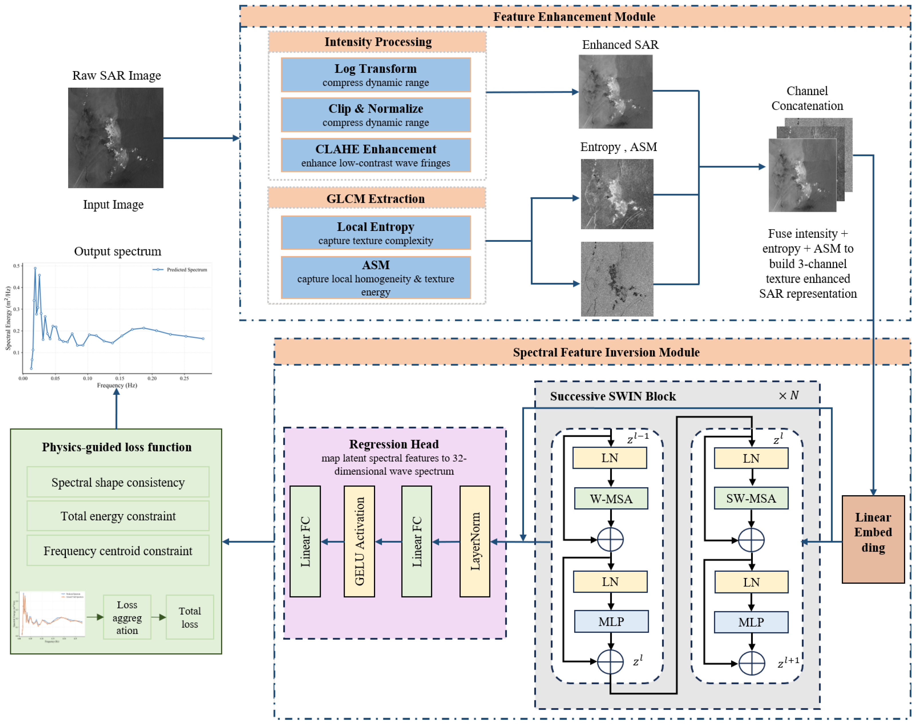
The workflow of the proposed PGT-Swin model is illustrated in Figure 1. The model is built on the Swin Transformer framework, which is suitable for high-dimensional physical parameter regression from remote sensing images. The framework consists of two main components, the feature enhancement module and the spectral inversion module. First, raw SAR images are processed by the feature enhancement module to generate multi-channel representations with explicit texture priors. Then, the spectral inversion module extracts hierarchical deep features and performs regression to obtain the 32-dimensional wave spectrum.

3.2. Image Preprocessing and Feature Enhancement

SAR images are inevitably disturbed by Speckle noise during the imaging process, and the texture of ocean waves is often hidden in the low-contrast background area. In order to enable the subsequent deep learning network to focus more efficiently on the wave-energy and orientation-sensitive texture features of ocean waves, this study designs a pre-feature Enhancement Module. As shown in Figure 1, this module mainly consists of three core steps: Intensity Processing, texture Extraction based on GLCM, and Channel Concatenation.

3.2.1. Intensity Processing

The original SAR image has an extremely high dynamic range. Direct input into the network is very likely to cause unstable gradients. Therefore, the intensity processing branch aims to standardize the image distribution and enhance local contrast, mainly including Log Transform, Clip & Normalize and CLAHE Enhancement.

To compress the dynamic range of the data and convert multiplicative noise into additive noise, a logarithmic transformation is first applied to the original pixel value $I_{raw}$:

$$I_{log}=10·lo{g}_{10}(I_{raw}+ϵ),$$

(1)

where $ϵ={10}^{-6}$ is a minimal constant to prevent logarithmic computation overflow. Then, the dynamic percentile clipping strategy is adopted to calculate the 2nd and 98th percentiles of $I_{log}$ (denoted as $P_2$ and $P_{98}$), and the outlier noise points in the extreme distribution are eliminated. Subsequently, the clipped data is linearly normalized to the range of $[0,1]$ and further mapped to an 8-bit unsigned integer format $[0,255]$:

$$I_{norm}={\displaystyle \frac{\mathrm{Clip}(I_{log},P_2,P_{98})-P_2}{P_{98}-P_2}}\times 255.$$

(2)

$\mathrm{Clip}(x,a,b)=\min \left\{\max \right(x,a),b\}$ limits x to the interval $[a,b]$. Finally, Contrast Limited Adaptive Histogram Equalization (CLAHE) is adopted to enhance the local contrast of $I_{norm}$. In this study, the clip limit was set to 3.0 and the tile grid size to 8 ∗ 8. This operation can effectively highlight the subtle wave crests and troughs hidden in the dark areas, and the output enhanced image is recorded as $I_{enhanced}$.

3.2.2. GLCM Extraction

The frequency spectrum of ocean waves essentially reflects the texture distribution characteristics of waves on the sea surface. To provide explicit physical texture priors to the network, the second branch of the module simulates the feature extraction process of the GLCM, extracting three key local texture feature maps from the preprocessed images.

Local entropy characterizes the complexity and information content of local textural patterns. The Shannon entropy within each local neighborhood is computed using a disk-shaped structuring element with a radius of 5, yielding the entropy map $I_{entropy}$, which effectively enhances the visualization of wave-breaking zones and complex intersecting wave systems. Homogeneity quantifies the uniformity of textural attributes across local image domains. In this study, a bilateral filter is utilized to characterize such textural homogeneity: it suppresses noise and smooths spatially uniform sea-surface regions while maintaining the sharpness of wave edges and discontinuities. Angular Second Moment (ASM) $I_{ASM}$ describes the uniformity and regularity of the grayscale distribution within an image. Herein, the local standard deviation is derived via a Laplacian-of-Gaussian (LoG) operator with Gaussian smoothing, and its reciprocal is adopted to approximate the ASM feature. A smaller local standard deviation (corresponding to higher energy) denotes more uniform and stable wave textural patterns in the respective region.

3.2.3. Channel Concatenation

In traditional visual models, single-channel grayscale images are usually constructed as three-channel inputs through simple replication, which not only leads to a waste of computing resources but also fails to provide additional information gain. In the final stage of this module, the traditional channel replication strategy was abandoned. Instead, the channel concatenation technology was adopted to fuse the outputs of the intensity processing branch and the texture extraction branch. Specifically, the model stacks the CLAHE-enhanced SAR image ($I_{enhanced}$), the local entropy feature map ($I_{entropy}$), and the homogeneity or ASM feature map in the channel dimension

$$C_{input}=\mathrm{Concat}(I_{enhanced},I_{entropy},I_{ASM}).$$

(3)

The operator $\mathrm{Concat}(·)$ denotes the concatenation of multiple feature maps along the channel dimension. This multi-channel fusion strategy ($3\times 448\times 448$) constructs a multi-dimensional feature space containing “intensity–complexity–uniformity” for the subsequent Swin Transformer network, enabling the network to retrieve the one-dimensional frequency spectrum. It can make full use of the statistical information of pixels and the spatial topological relationship.

3.3. Swin Transformer Architecture and Physics-Informed Optimization

3.3.1. Swin Transformer Feature Extraction Block

The core feature extraction network of this study adopts the Swin Transformer architecture. Different from the traditional global ViT, the Swin Transformer introduces the local window self-attention mechanism and hierarchical network structure. While significantly reducing the computational complexity, it can effectively extract the texture features of waves of different scales in SAR images. The basic building blocks of the Swin Transformer usually appear in pairs. Two successive Swin Transformer blocks are mainly composed alternately of Layer Normalization (LN), Multi-Layer Perceptron (MLP), and two different multi-head self-attention modules: Window-based Multi-head Self-Attention (W-MSA) and Shifted Window-based Multi-head Self-Attention (SW-MSA).

When traditional ViT calculates global self-attention, its computational complexity is in a square relationship with the image size, which will lead to a huge consumption of video memory when processing high-resolution SAR images. To solve this problem, Swin Transformer adopts the window segmentation strategy, as follows:

$$\mathsf{\Omega }\left(MSA\right)=4hw{C}^2+2{\left(hw\right)}^{2}C,$$

(4)

$$\mathsf{\Omega }(W-MSA)=4hw{C}^2+2M^{2}hwC,$$

(5)

where $\mathsf{\Omega }(·)$ denotes the computational complexity; h and w denote the height and width of the feature map, respectively; C is the number of channels; and M is the side length of each local attention window. MSA and W-MSA refer to global multi-head self-attention and window-based multi-head self-attention, respectively.

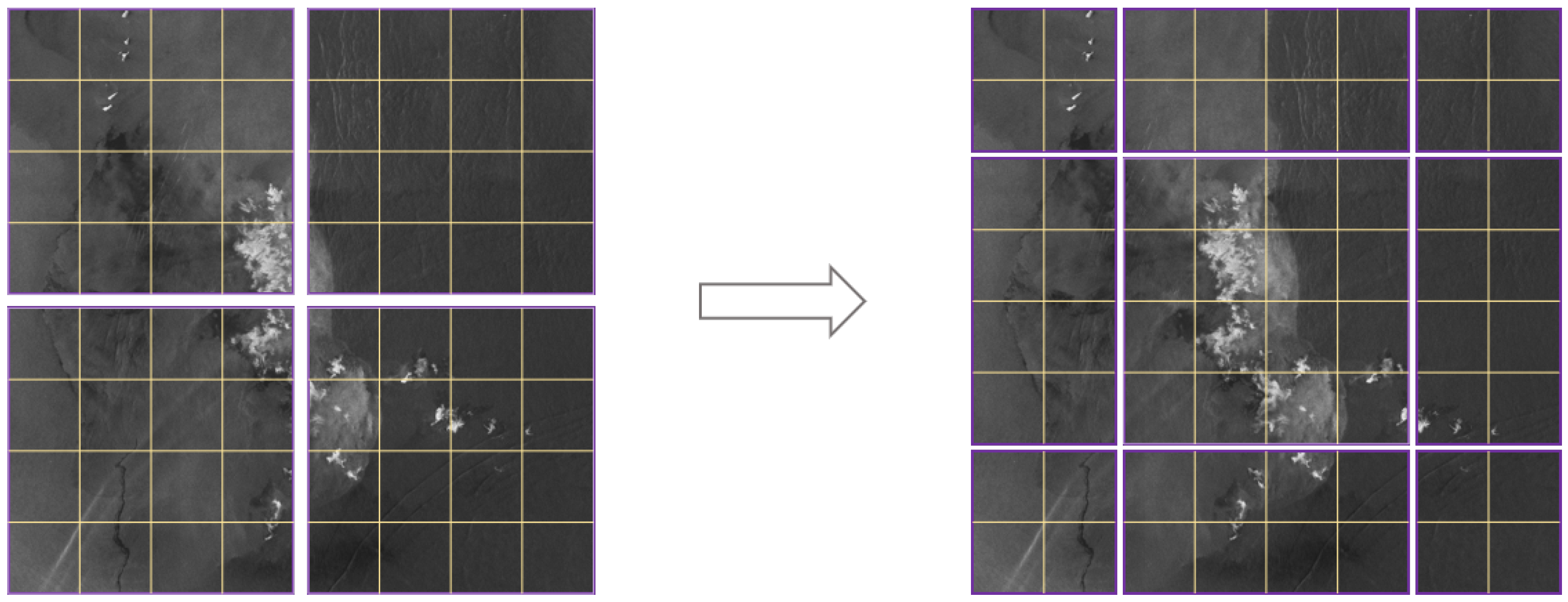
As illustrated in Figure 2, the input feature map is partitioned into non-overlapping local windows of equal size. During W-MSA, self-attention is computed independently within each window. This partitioning reduces the attention-related complexity from $2{\left(hw\right)}^{2}C$ to $2M^{2}hwC$, making it linear rather than quadratic with respect to the number of spatial positions when the window size is fixed. However, restricting self-attention to individual windows prevents direct information exchange across window boundaries. This limitation can hinder the representation of spatially continuous wave patterns and energy distributions that extend across large regions in SAR imagery. To address this issue, the subsequent layer applies shifted-window multi-head self-attention, in which the window partition is shifted by half the window size along both spatial dimensions. The shifted partition allows each new window to cover patches that belonged to different windows in the preceding layer, thereby enabling information exchange between neighboring regions. Alternating W-MSA and SW-MSA preserves the computational efficiency of local attention while progressively enlarging the effective receptive field. This design helps the model represent both local high-frequency textures and large-scale low-frequency variations in SAR ocean-wave imagery.

3.3.2. Physics-Informed Spectral Loss Function

In the retrieval task of the wave frequency spectrum, the traditional single Mean Squared Error ($MSE$) often can only punish the prediction deviation at the numerical level while ignoring the inherent physical characteristics and spatial distribution laws of the wave spectrum. In order to guide the model to learn an energy distribution that is not only numerically accurate but also conforms to the laws of ocean Physics, this study proposes a physics-informed Spectral Loss function [59]. This loss function combines numerical approximation in the logarithmic domain with physical momentum constraints in the linear domain. Its overall objective function ${\mathcal{L}}_{Total}$ is defined as:

$${\mathcal{L}}_{Total}={\mathcal{L}}_{MSE}+{\mathcal{L}}_{Cos}+{\mathcal{L}}_{Energy}+{\mathcal{L}}_{Centroid}.$$

(6)

Due to the large energy span of the wave spectrum, the model is directly fitted in the logarithmic domain to ensure the stability of the values. In the logarithmic domain, we simultaneously constrained the absolute error of the predicted values and the shape similarity. $MSE$ serves as the fundamental numerical constraint to punish the absolute difference between the logarithmic spectrum ${\widehat{S}}_{log}$ output by the network and the true logarithmic spectrum $S_{log}$:

$${\mathcal{L}}_{MSE}={\displaystyle \frac{1}{B·N}}{\displaystyle \sum _{i=1}^B}{\displaystyle \sum _{j=1}^N}{\left({\widehat{S}}_{log}^{(i,j)}-S_{log}^{(i,j)}\right)}^2,$$

(7)

where B represents the batch size and N represents the dimension of the frequency spectrum. Then, we introduced cosine similarity loss to enable the model to capture the peak positions and overall trends of the wave spectrum more accurately. This loss constrains structural consistency by calculating the angle between the predicted spectral vector and the true spectral vector in a high-dimensional space:

$${\mathcal{L}}_{Cos}={\displaystyle \frac{1}{B}}{\displaystyle \sum _{i=1}^B}\left(1-{\displaystyle \frac{{\widehat{S}}_{log}^{\left(i\right)}·S_{log}^{\left(i\right)}}{\parallel {\widehat{S}}_{log}^{\left(i\right)}\parallel \parallel S_{log}^{\left(i\right)}\parallel }}\right).$$

(8)

In addition, to introduce the prior knowledge of oceanography, we restore the prediction results in the logarithmic domain to the linear domain for physical momentum calculation. The mapping relationship is defined as:

$$S={\displaystyle \frac{\mathrm{ReLU}(\exp \left(S_{log}\right)-1)}{\mathrm{10,000}}},$$

(9)

where the $\mathrm{ReLU}\left(x\right)=\max (0,x)$ activation function ensures the nonnegative spectral energy density. The zero-order moment ($m_0$) of the wave spectrum represents the total area under the spectrum, whose physical meaning directly corresponds to the total energy of the wave and is proportional to the square of SWH. To ensure energy conservation, the L1 norm is adopted to compare the total energy differences, thereby enhancing the model’s robustness against outliers:

$${\mathcal{L}}_{Energy}={\displaystyle \frac{1}{B}}{\displaystyle \sum _{i=1}^B}\left|{\displaystyle \sum _{j=1}^N}{\widehat{S}}^{(i,j)}-{\displaystyle \sum _{j=1}^N}{S}^{(i,j)}\right|.$$

(10)

The first-order moment of the wave spectrum reflects the distribution center of energy at frequency, whose physical significance is closely related to the average wave period. To ensure the consistency of energy propagation characteristics, constraints are imposed by calculating the centroid difference between the predicted spectrum and the true spectrum:

$${\mathcal{L}}_{Centroid}={\displaystyle \frac{1}{B}}{\displaystyle \sum _{i=1}^B}\left|{\displaystyle \frac{{\sum }_{j=1}^N({\widehat{S}}^{(i,j)}·f_j)}{{\sum }_{j=1}^N{\widehat{S}}^{(i,j)}+\epsilon }}-{\displaystyle \frac{{\sum }_{j=1}^N(S^{(i,j)}·f_j)}{{\sum }_{j=1}^N{S}^{(i,j)}+\epsilon }}\right|,$$

(11)

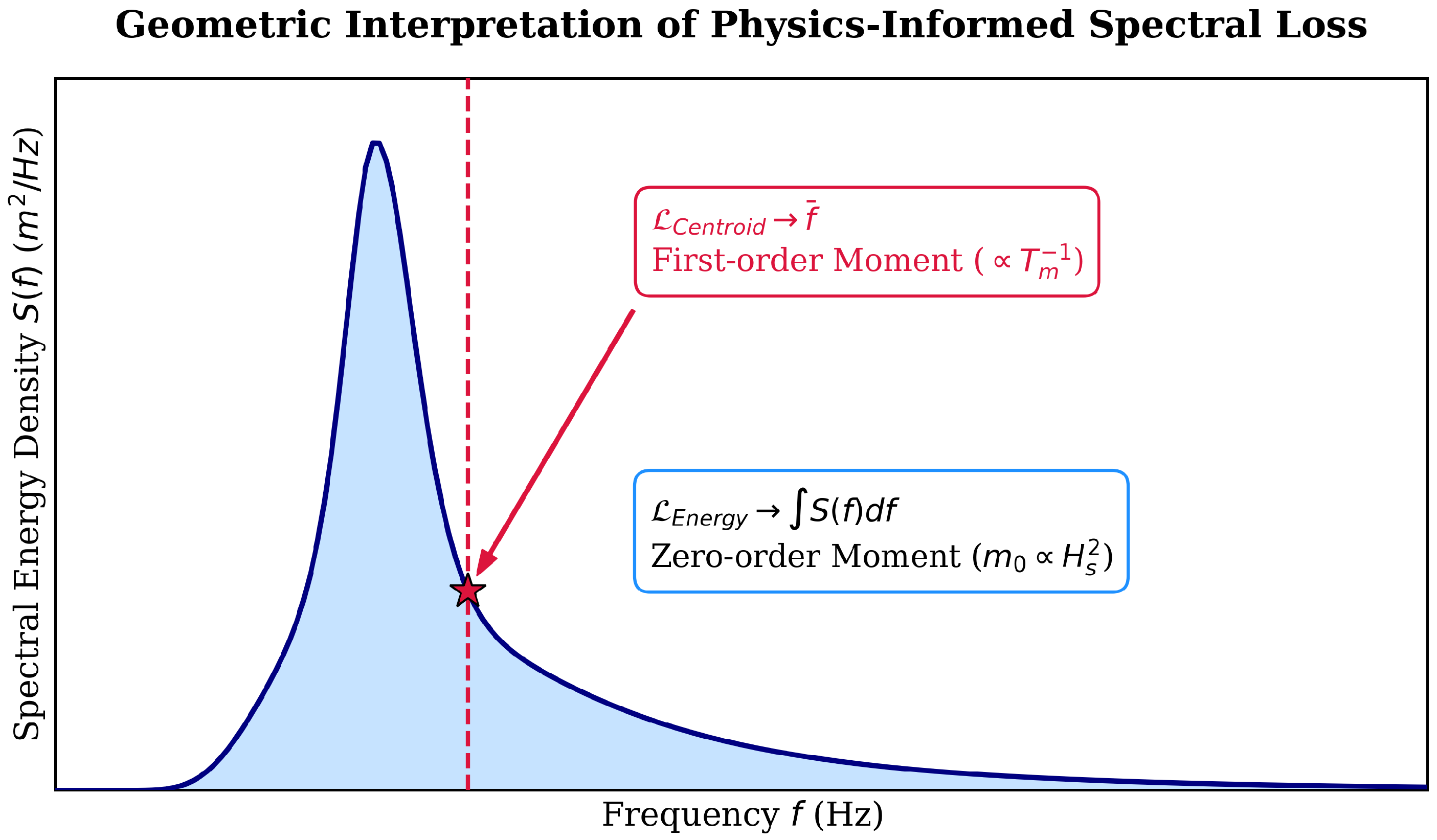
where $f_j$ is the frequency index vector of the jth dimension, $ϵ$ is a minimal positive number that prevents division-by-zero anomalies, and we let it be ${10}^{-6}$. As shown in Figure 3, it is the physical prior loss function.

The four loss components have complementary functions. ${\mathcal{L}}_{MSE}$ controls the pointwise reconstruction error in the logarithmic domain, while ${\mathcal{L}}_{Cos}$ preserves the overall spectral shape independently of spectral magnitude. After conversion to the linear domain, ${\mathcal{L}}_{Energy}$ constrains the integrated spectral energy associated with SWH, and ${\mathcal{L}}_{Centroid}$ constrains the energy-weighted position of the frequency distribution. Thus, the numerical losses regulate bin-wise agreement and spectral-shape similarity, whereas the physics-guided losses regulate physically interpretable integral properties of the reconstructed spectrum.

4. Results

We evaluate the proposed PGT-Swin model through ablation studies and comparative experiments on publicly available Sentinel-1 SAR images collocated with CFOSAT SWIM wave spectrum. First, we give a brief introduction to the benchmark datasets and describe the preprocessing. Next, we elaborate on the details of the implementation, covering the network architecture, shifted-window Swin Transformer backbone, physics-guided spectral loss functions, and training configuration. Subsequently, we validate the competitiveness of PGT-Swin by comparing its wave spectrum retrieval performance, as well as derived SWH and MWP, with several baseline models. Ablation tests are then performed to assess the contribution of three essential components: the texture-enhancement module based on GLCM features and the physics-guided spectral constraints. Finally, we discuss the limitations of the PGT-Swin model, analyze the reasons for lower MWP retrieval accuracy, and suggest potential improvements for future work.

4.1. Dataset

Our first contribution is to construct a reliable dataset for the supervised training of the inversion model, a rigorous spatiotemporal collocation was performed between the Sentinel-1 (S-1) SAR imagery and China-France Oceanography Satellite (CFOSAT) Surface Waves Investigation and Monitoring (SWIM) measurements. The imagery acquired from 1 to 31 May 2025 and the study area covers the South China Sea, bounded by 6–22°N and 105–122°E. The center latitude, longitude, and azimuth time were parsed from the associated annotation XML files. The CFOSAT Level-2 wave spectra database was subsequently queried to find measurements that strictly enveloped the SAR acquisition time ($t_{start}\le t_{SAR}\le t_{end}$). Spatial collocation was then achieved by calculating the minimum Euclidean distance between the SAR geometric center and the CFOSAT footprints, implemented efficiently on GPUs utilizing the cuDF library.

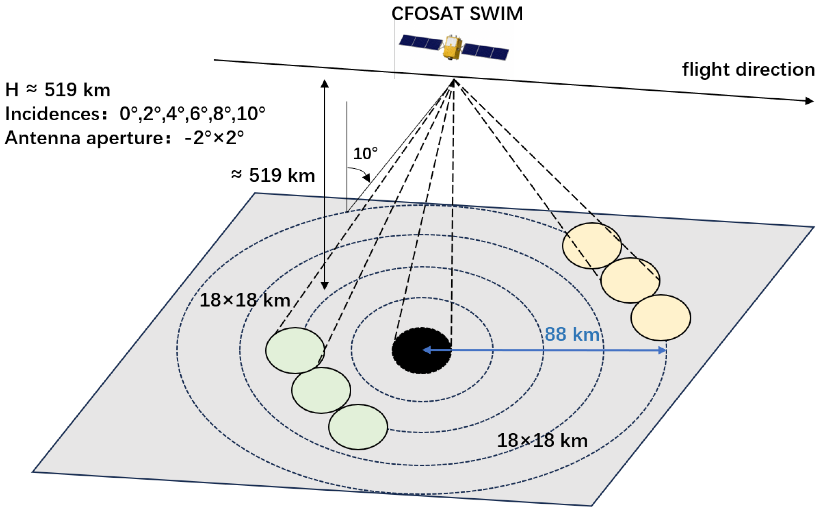
The primary wave-observation payload aboard CFOSAT is the Surface Waves Investigation and Monitoring (SWIM) instrument, a Ku-band real-aperture radar employing a rotating, multi-incidence scanning geometry. As shown in Figure 4, CFOSAT operates at an altitude of approximately 519 km. SWIM sequentially observes the sea surface using six beams with incidence angles of $0^{\circ }$ (nadir), $2^{\circ }$, $4^{\circ }$, $6^{\circ }$, $8^{\circ }$, and ${10}^{\circ }$, each with an antenna beamwidth of approximately $2^{\circ }\times 2^{\circ }$. The elementary footprint of an off-nadir beam is approximately $18\mathrm{km}\times 18\mathrm{km}$, while the outermost ${10}^{\circ }$ beam reaches approximately 88 km from the subsatellite track. Successive overlapping scans are combined into Level-2 spectral boxes with a spatial scale of approximately 70–90 km. This rotating conical-scanning configuration enables SWIM to retrieve wave spectra on both sides of the satellite track over a nominal wavelength range of approximately 70–500 m. Although reported error sources include radar speckle noise, low-wavenumber parasitic peaks and noise floors, incomplete representation of short-wavelength components outside the observable band, directional ambiguity, and spatial averaging within the relatively large spectral boxes [60,61,62]. SWIM products have been evaluated against numerical wave models, such as ECMWF WAM and MFWAM, in situ buoy observations, and independent satellite measurements including Jason-3 [60,63]. Additional spectrum-level comparisons with buoy measurements have shown that the $8^{\circ }$ and ${10}^{\circ }$ beams provide good spectral consistency [61,64]. A validation using spectra from 98 NDBC buoys further reported that the ${10}^{\circ }$ beam generally provided a reliable estimate of total spectral energy [62]. The products are considered reliable for quality-controlled observations in spatially homogeneous, open ocean. Therefore, we can regard the spectra of SWIM as the reference spectra.

SWIM provides dedicated wave-spectrum products, but only within the spatial and temporal sampling of the CFOSAT mission. Because CFOSAT and SAR missions differ in their orbits, acquisition times, and viewing geometries, an individual SAR scene may not have a concurrent SWIM spectrum. SWIM products, therefore, cannot provide frequency-resolved information for SAR acquisitions outside CFOSAT overpasses or for SAR archives predating the CFOSAT mission. This study does not seek to reproduce SWIM products where they are already available or to replace SWIM observations. Instead, collocated SAR and SWIM data are used to learn a cross-sensor mapping from SAR image features to SWIM-referenced frequency spectra. Once trained, the proposed model is intended to estimate a SWIM-referenced frequency spectrum from a SAR image when no concurrent SWIM spectrum is available, thereby extending frequency-resolved sea-state characterization to SAR-only acquisitions.

4.2. Implementation Details

To ensure stable gradient propagation and prevent vanishing gradients caused by the minuscule magnitude of wave energy densities, the matched 32-dimensional 1D frequency spectra S were scaled and transformed into the logarithmic domain:

$$S_{log}=\ln (1+S\times \mathrm{10,000}).$$

(12)

The successfully collocated dataset was then randomly partitioned into a training set (70%) and a testing set (30%). A fixed random seed (Seed = 42) was maintained throughout the data splitting and initialization processes to ensure rigorous reproducibility. After training and testing, we used the SAR images and ERA5 data of the Drake Passage 54–62°S and 60–70°W from 2025 January to February for independent verification of different ocean regions and seasons.

The model was implemented using the PyTorch 2.8.0 framework. To accelerate training and reduce memory footprint, Automatic Mixed Precision (AMP), coupled with a gradient scaler, was utilized. The network was optimized using the AdamW optimizer with a weight decay of $1\times {10}^{-4}$. To preserve the pre-trained representation capabilities of the Swin Transformer while adapting to the regression task, a layer-wise learning rate strategy was adopted: the Swin backbone was fine-tuned with a lower learning rate of $1\times {10}^{-5}$, whereas the randomly initialized regression head was trained with a higher learning rate of $1\times {10}^{-4}$. A ReduceLROnPlateau scheduler was employed to dynamically decay the learning rate by a factor of 0.5 if the validation loss stagnated for five epochs. Gradient clipping with a maximum norm of 5.0 was applied to prevent exploding gradients. The batch size was set to 16. An early stopping mechanism was configured to halt training if no improvement was observed over 30 consecutive epochs. Given the complex interplay between the numerical and physical loss components, a random search strategy was implemented for Hyperparameter Optimization (HPO) rather than a rigid grid search.

Two wave-integral parameters were employed to better demonstrate the characteristics and accuracy of ocean wave spectra retrieval, including SWH and MWP. Two integral wave parameters, SWH and MWP, were used to evaluate the physical consistency of the retrieved spectra. These parameters describe the overall energy level and characteristic period of ocean waves, respectively. They were calculated from the retrieved wave spectrum $S\left(f\right)$ as follows:

$$H_s=4\sqrt{\int S(f)df},$$

(13)

$$T_{m02}=\sqrt{{\displaystyle \frac{\int S(f)df}{\int f^{2}S(f)df}}}.$$

(14)

The SWH and MWP are denoted as $H_s$ and $T_{m02}$, and after the model inverted the wave spectrum, we performed calculations to obtain SWH and MWP.

4.3. Experimental Results on PGT-Swin

To evaluate the performance of the proposed model, we analyzed the results from two aspects. First, we examined whether the model could accurately reconstruct the wave spectrum from SAR images. This evaluation directly reflects the model’s ability to learn the spectral energy distribution. Second, we calculated the SWH and MWP from the retrieved spectra through spectral integration. These two parameters were then compared with the ground-truth values to further assess the physical reliability of the retrieved spectra. 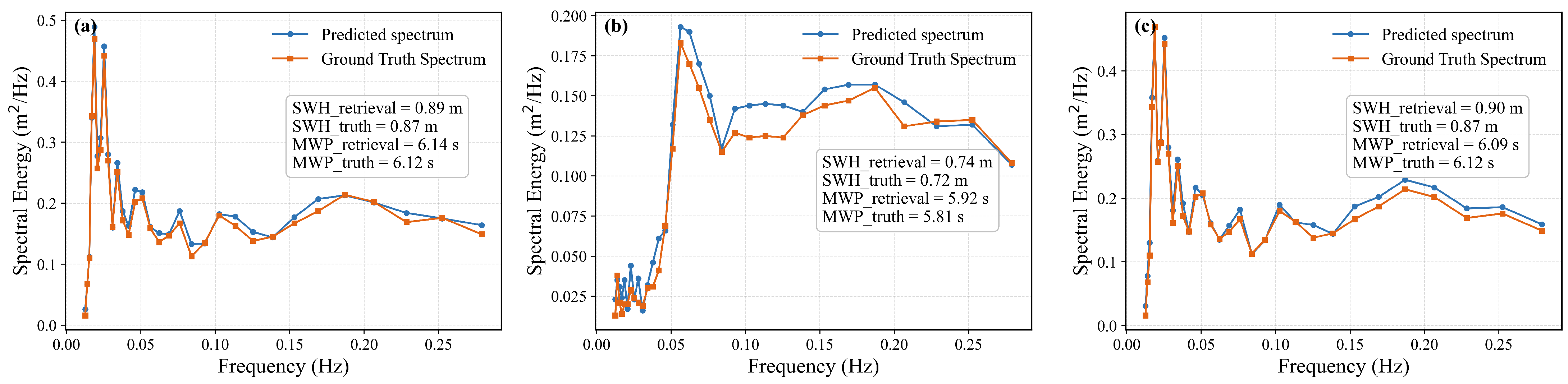Figure 5 shows representative examples of the one-dimensional frequency spectra retrieved by the proposed model. The blue curves denote the retrieved spectra, and the orange curves denote the ground-truth spectra. Overall, the proposed model can effectively reproduce the main shape of the wave spectrum under different spectral patterns. In particular, the model captures the dominant energy peak, the general spectral trend, and the decay behavior in the high-frequency region. These results indicate that the proposed method can learn the relationship between SAR image features and the corresponding wave spectral distribution.

Table 1. Comparison of spectrum-level reconstruction performance among different models.

Method	Spectral MAE	Spectral Correlation
Swin	0.0179	0.7275
ViT	0.0158	0.8100
SAR-WaveInv	0.0169	0.8328
ResNet	0.0172	0.7832
PGT-Swin	0.0139	0.8500

compares the spectrum-level reconstruction performance of different models. PGT-Swin achieves the lowest spectral MAE of 0.0139, representing a reduction of approximately 12.0% compared with the best-performing baseline, ViT (0.0158). It also obtains the highest spectral correlation of 0.8500, exceeding that of SAR-WaveInv (0.8328), the strongest baseline for this metric. These results demonstrate that PGT-Swin reduces pointwise spectral reconstruction errors while preserving greater consistency with the reference spectral shape, thereby confirming the effectiveness of the proposed texture-enhancement and physics-guided learning strategy.

Based on the retrieved wave spectra, SWH and MWP were further derived using spectral integration.

Table 2. Comparison of SWH and MWP retrieval performance among different models.

Feature	Method	MSE	MAE	R2
SWH (m)	Swin	0.0027	0.0393	0.9183
	ViT	0.0019	0.0354	0.9439
	SAR-WaveInv	0.0019	0.0354	0.9428
	CNN-SWH	0.0024	0.0377	0.9291
	ResNet	0.0024	0.0381	0.9288
	DenseNet	0.0019	0.0345	0.9431
	EfficientNet	0.0018	0.0306	0.9452
	PGT-Swin	0.0014	0.0327	0.9591
MWP (s)	Swin	0.0736	0.1957	0.1653
	ViT	0.0590	0.1554	0.3310
	SAR-WaveInv	0.0632	0.1479	0.2825
	CNN-SWH	0.0705	0.1736	0.2004
	ResNet	0.0524	0.1532	0.3166
	DenseNet	0.1008	0.1967	−0.1438
	EfficientNet	0.0691	0.1747	0.1736
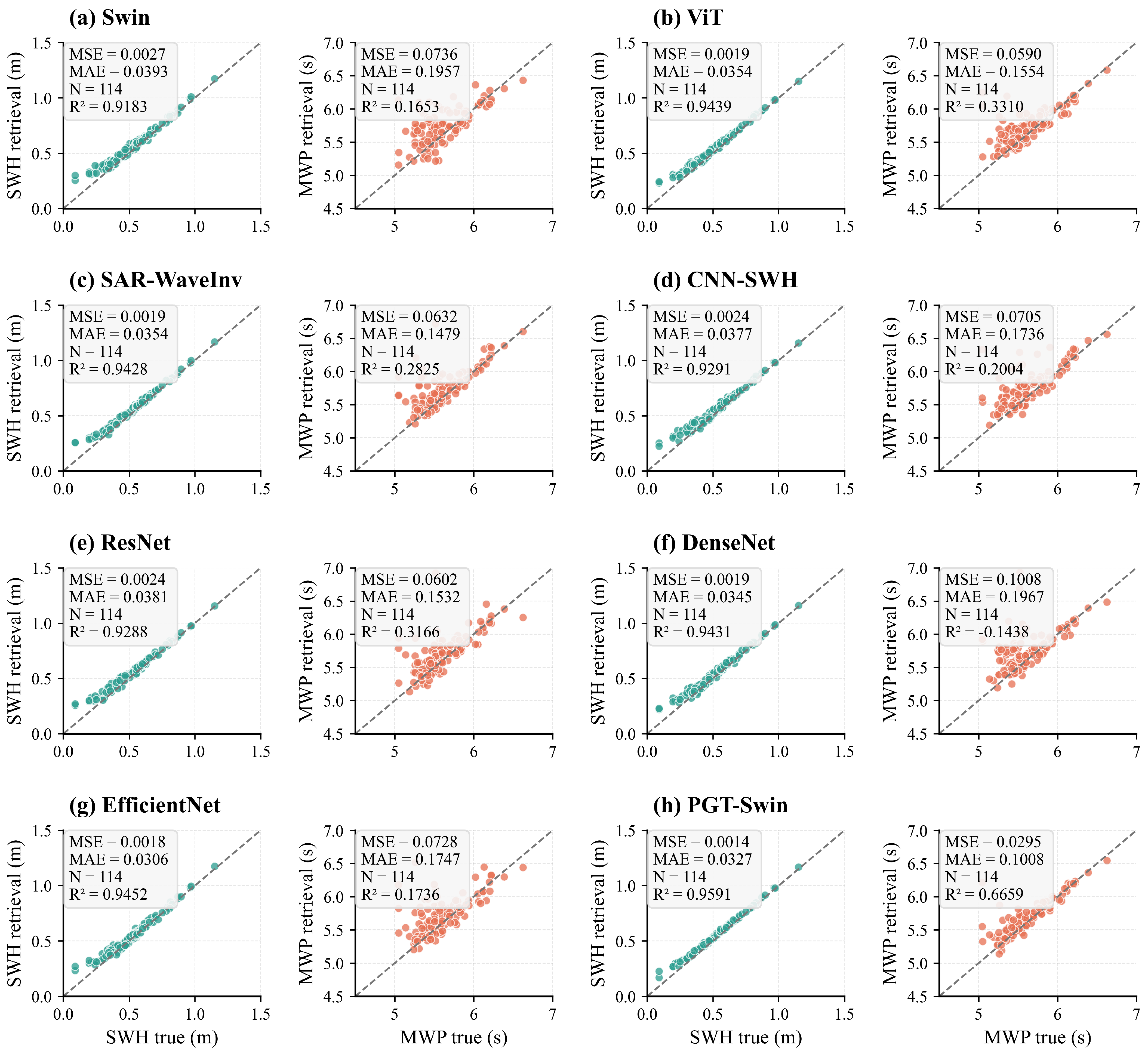
	PGT-Swin	0.0295	0.1008	0.6659

summarizes the quantitative comparison between PGT-Swin and other baseline models, including Swin, ViT, SAR-WaveInv, CNN-SWH, ResNet, DenseNet, and EfficientNet. For SWH retrieval, PGT-Swin achieves the best overall performance, with an MSE of 0.0014, a $MAE$ of 0.0327 m, and an $R^2$ of 0.9591. Although EfficientNet obtains the lowest $MAE$ value of 0.0306 m, PGT-Swin achieves a higher $R^2$, which indicates stronger consistency with the ground-truth SWH values. This result demonstrates that the proposed model can accurately preserve the total spectral energy, which is directly related to SWH.

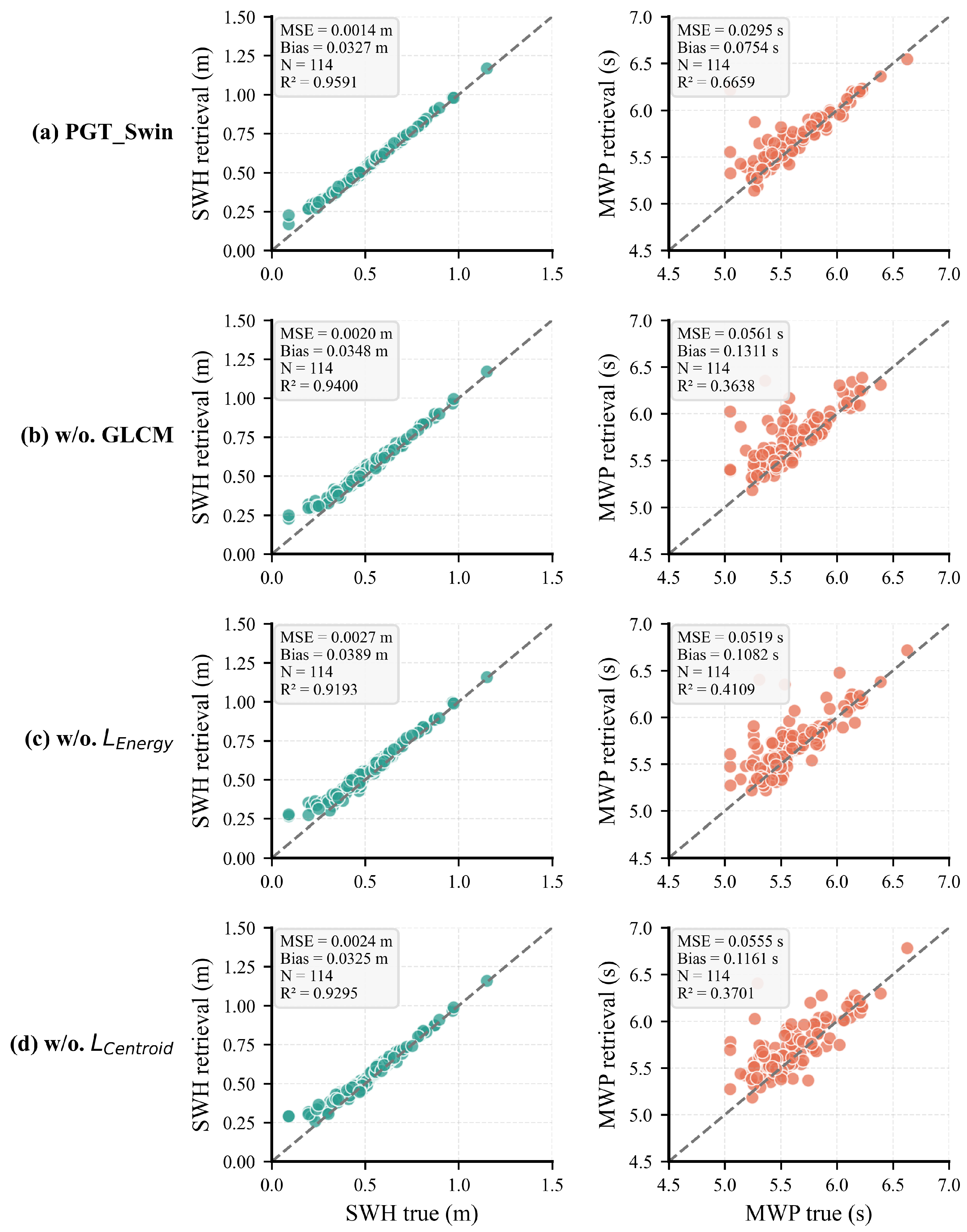
For MWP retrieval, PGT-Swin also shows the best performance among all models, with an $MSE$ of 0.0295, a $MAE$ of 0.1008 s, and an $R^2$ of 0.6659. Compared with the basic Swin model, the $MSE$ decreases from 0.0736 to 0.0295, and the $R^2$ increases from 0.1653 to 0.6659. This improvement indicates that the proposed GLCM-based texture enhancement and physics-guided spectral constraints can effectively improve the estimation of wave-period-related parameters. Compared with CNN-based models, such as ResNet, DenseNet, EfficientNet, and CNN-SWH, PGT-Swin also achieves more stable performance. This suggests that the shifted-window attention mechanism is beneficial for capturing both local wave textures and global periodic structures in SAR images.

Figure 6 further shows the scatter comparison of SWH and MWP retrieval results for different models. The left subplots of each model show SWH retrieval results, and the right subplots show MWP retrieval results. For SWH, most samples predicted by PGT-Swin are tightly distributed around the 1:1 line, showing strong agreement between retrieved and ground-truth values. Other baseline models also show reasonable SWH retrieval ability, but their point distributions are generally more dispersed than that of PGT-Swin. For MWP, the differences among models are more obvious. PGT-Swin produces the most concentrated distribution near the 1:1 line, while other models show larger deviations and stronger dispersion.

It should be noted that the MWP retrieval accuracy is generally lower than the SWH retrieval accuracy. This phenomenon is mainly related to the different physical meanings and calculation mechanisms of the two parameters. SWH is determined by the zeroth-order moment of the wave spectrum, which reflects the total spectral energy. Therefore, as long as the model can accurately reconstruct the overall energy level of the spectrum, SWH can be estimated with high accuracy. In contrast, MWP is determined by the ratio between the zeroth-order and second-order spectral moments. It is more sensitive to the detailed distribution of energy along the frequency axis. Small errors in the reconstructed spectrum may have a limited influence on the total spectral energy, but they can significantly affect the spectral moment related to frequency. In particular, deviations near the peak frequency or in the high-frequency tail may lead to clear changes in MWP. In addition, the dynamic range of MWP in the test set is relatively narrow. When the variation range of the true values is small, even a small absolute error can cause a noticeable decrease in $R^2$. Therefore, the lower $R^2$ of MWP does not necessarily indicate that the absolute retrieval error is large. Instead, it shows that MWP is more sensitive to spectral-shape errors and frequency-distribution deviations than SWH.

The experimental results demonstrate that PGT-Swin can effectively retrieve wave spectra from SAR images and further derive reliable energy-related wave parameters. The high SWH accuracy confirms that the proposed model can preserve the total wave energy of the reconstructed spectrum. The improved MWP performance shows that the model can also capture frequency-distribution information to a certain extent. These results indicate that PGT-Swin provides a physically meaningful and accurate solution for SAR-based wave spectrum retrieval and ocean-wave monitoring.

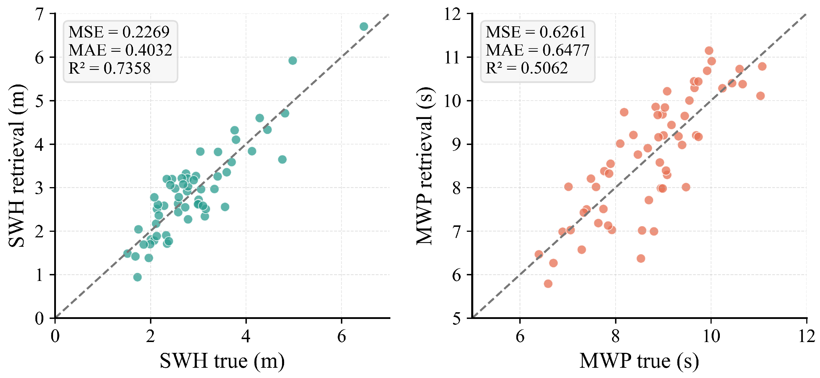
We further validated PGT-Swin using an independent external ERA5 dataset collected in the Drake Passage during January and February 2025. It contains 59 matched observations representing moderate-to-energetic sea states, with reference SWH values ranging from 1.52 to 6.47 m and MWP values ranging from 6.39 to 11.07 s. As shown in Figure 7, PGT-Swin achieved an $MSE$ of 0.2269, an $MAE$ of 0.4032, and an $R^2$ of 0.7358 for SWH. For MWP, the corresponding $MSE$, $MAE$, and $R^2$ were 0.6261, 0.6477, and 0.5062, respectively. Although performance declined relative to the randomly partitioned in-domain test set, the model remained able to retrieve wave parameters in a geographically distinct region under higher-energy sea states. These results suggest some capacity to generalize across regions and seasons. The evaluation also covered SWH values up to approximately 6.5 m. The greater scatter in the MWP estimates, however, suggests that period retrieval is more sensitive to regional and sea-state shifts. Additional evaluation using severe storm events, collocated wind-speed measurements, and observations from independent buoys is needed to assess the model’s robustness under these conditions.

4.4. Ablation Experiments

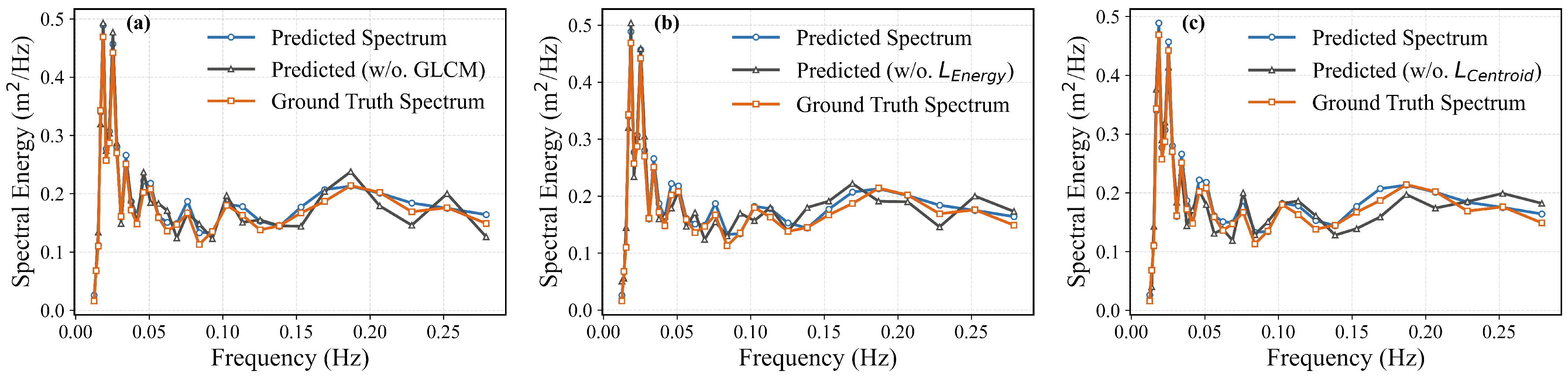
Figure 8 reports inversion results of the wave spectrum, comparing the complete model with variants obtained by removing specific modules (i.e., “w/o.”) while keeping all other settings identical. It can be seen that removing any module will introduce deviations at the main peak position and the high-frequency tail, indicating that each module contributes to the spectral shape reconstruction.

As shown in Figure 8a, although the variant model lacking GLCM texture enhancement can roughly capture the contour of the spectrum, obvious overfitting and oscillation occur in the high-frequency tail and the peak area with sharp energy fluctuations. This verifies that models relying solely on a single intensity information are difficult to parse complex local wave textures, resulting in poor subsequent inversion effects of wave parameters. However, the introduction of GLCM features effectively enhances the model’s perception ability for detailed high-frequency information.

Table 3. Comparative performance of ablation analysis on SWH and MWP.

Feature	Method	MSE	MAE	R2
SWH (m)	w/o. GLCM	0.0020	0.0351	0.9400
	w/o. ${\mathcal{L}}_{Energy}$	0.0027	0.0403	0.9193
	w/o. ${\mathcal{L}}_{Centroid}$	0.0024	0.0350	0.9295
	PGT-Swin	0.0014	0.0327	0.9591
MWP (s)	w/o. GLCM	0.0561	0.1574	0.3638
	w/o. ${\mathcal{L}}_{Energy}$	0.0519	0.1505	0.4109
	w/o. ${\mathcal{L}}_{Centroid}$	0.0555	0.1661	0.3701
	PGT-Swin	0.0295	0.1008	0.6659

and Figure 9 detail $MSE$, $MAE$ and $R^2$ of different ablation variants on the two macroscopic integral physical quantities SWH and MWP. According to the linear wave theory, the $m_0$ of the wave spectrum is proportional to the square of the SWH. The data indicates that when the ${\mathcal{L}}_{Energy}$ constraint is removed, the inversion performance of SWH shows the most significant decline, with its $MSE$ surging from 0.0014 of the complete model to 0.0027. The value of $R^2$ sharply declined from 0.9591 to the lowest of 0.9193 in this group. This fully demonstrates that ${\mathcal{L}}_{Energy}$ plays a substantial contribution in constraining the network output to conform to the conservation of total energy and thereby achieving high-precision wave height inversion.

MWP is extremely sensitive to the center of the frequency distribution. As shown in Table 3, the removal of ${\mathcal{L}}_{Centroid}$ caused the $R^2$ of MWP to drop sharply to 0.3701, indicating that when the network lacks first-order moment constraints, it is highly prone to serious misjudgment of the average wave propagation period. Meanwhile, the removal of GLCM features dealt the most fatal blow to MWP ($R^2$ dropped to 0.3638, $MSE$ rose to 0.0561). This indicates that the accurate inversion of MWP is highly dependent on the clear spatial frequencies of wave fringes in SAR images, and the local entropy and homogeneity features provided by GLCM offer crucial explicit texture priors for the network to capture these spatial frequencies.

Overall, the comparison with the Swin baseline demonstrates that the improvement of the proposed method does not derive only from the backbone network. Instead, the GLCM module and the physics-guided loss functions provide complementary contributions. The GLCM module enhances the representation of local wave texture information, while ${\mathcal{L}}_{Energy}$ and ${\mathcal{L}}_{Centroid}$ guide the reconstructed spectrum to satisfy energy conservation and frequency-distribution consistency. Their combination enables the model to achieve more accurate and physically reliable inversion results.

4.5. Preliminary Wave-Energy Resource Characterization

To quantitatively investigate the relevance of the retrieved frequency spectra to wave-energy applications, the wave-energy density, energy period, and wave-energy flux were derived from both the retrieved and reference spectra. For a one-dimensional sea-surface-elevation frequency spectrum, $S\left(f\right)$, the (n)-th-order spectral moment is defined as

$$m_n={\int }_{f_{\min }}^{f_{\max }}{f}^{n}S\left(f\right)df,$$

(15)

where $f_{\min }$ and $f_{\max }$ denote the lower and upper limits of the retrieved frequency range. The total wave-energy density per unit sea-surface area can then be calculated as

$$E={\rho }_{w}g{m}_0={\displaystyle \frac{{\rho }_{w}g{H}_s^2}{16}},$$

(16)

where E is expressed in J/m², ${\rho }_w=1025$ kg/m³ is the seawater density, and $g=9.81$ m/s² is the gravitational acceleration. The energy period is calculated from the negative first-order spectral moment as

$$T_e={\displaystyle \frac{m_{-1}}{m_0}}.$$

(17)

The wave-energy flux per unit wave-crest width is generally expressed as

$$P={\rho }_{w}g{\int }_{f_{\min }}^{f_{\max }}{C}_g(f,h)S\left(f\right)df,$$

(18)

where $C_g(f,h)$ is the frequency- and water-depth-dependent group velocity. Under deep-water conditions, $C_g=g/\left(4\pi f\right)$, and the wave-energy flux can be simplified as

$$P={\displaystyle \frac{{\rho }_w{g}^2}{4\pi }}{m}_{-1}={\displaystyle \frac{{\rho }_w{g}^2}{64\pi }}{H}_s^2{T}_e,$$

(19)

where P is expressed in W/m and is converted to kW/m in the subsequent analysis. For each matched sample, E, $T_e$, and P were independently calculated from the retrieved and reference spectra.

Table 4. Descriptive statistics of the reference and retrieved wave-energy parameters.

Quantity	Reference				Retrieved
	Mean	Std.	Min.	Max.	Mean	Std.	Min.	Max.
Energy density ($\mathrm{J}/{\mathrm{m}}^2$)	188.3816	134.2551	5.0547	832.4768	207.5757	134.3078	18.3423	857.2961
Energy period $T_e$ ($\mathrm{s}$)	8.0277	1.2046	6.0626	13.1620	8.5970	1.0445	7.1781	12.9451
Wave power ($\mathrm{kW}/\mathrm{m}$)	1.2500	1.0587	0.0239	6.0253	1.4258	1.0625	0.1558	6.2664

shows the descriptive statistics of the reference and retrieved wave-energy parameters. Moreover, $T_e=m_{-1}/m_0$ should be distinguished from the MWP $T_{m02}=\sqrt{m_0/m_2}$; the two periods represent different spectral moments and are not interchangeable.

The total wave-energy density can be derived from SWH, while the total deep-water wave-power flux can be estimated from SWH and the energy period. These integrated quantities, however, do not show how energy is distributed across frequencies. The reconstructed spectrum allows the energy and power contributions of individual frequency bands to be evaluated. As reported in

Table 5. Frequency-band evaluation of the energy distribution and wave-power contributions derived from the retrieved and SWIM-referenced spectra.

Frequency Band	Energy-Fraction MAE	Energy RMSE (J/m2)	Energy Correlation	Power MAE (kW/m)	Power RMSE (kW/m)
Low frequency	0.0208	5.1819	0.8390	0.1058	0.1096
Intermediate frequency	0.0182	6.3479	0.8612	0.0385	0.0427
High frequency	0.0249	9.4997	0.8435	0.0311	0.0346

, the energy-fraction MAEs for the low, intermediate, and high-frequency bands are 0.0208, 0.0182, and 0.0249, respectively. These values correspond to errors of approximately 1.82–2.49 percentage points. The correlations between the retrieved and reference band-limited energies exceed 0.8 for all three bands, showing that the model tracks sample-to-sample changes in spectral energy allocation. The error pattern differs between energy and wave power. The high-frequency band has the largest energy RMSE of 9.4997, whereas the low-frequency band has the largest wave-power MAE of 0.1058. This difference follows from the deep-water group velocity, $C_g=g/\left(4\pi f\right)$, which assigns greater weight to low-frequency components when calculating energy flux. The reconstructed spectrum, therefore, provides frequency-resolved information that is absent from SWH and representative-period descriptions, including how energy is allocated among frequency bands and which bands make the largest contributions to wave-power flux.

The descriptive statistics in Table 4 nevertheless reveal a systematic positive bias in the retrieved energy-related quantities. Relative to the SWIM-referenced values, the retrieved mean energy density is higher by 19.1941, corresponding to a relative bias of 10.19%; the mean energy period is overestimated by 0.5693 s, or 7.09%; and the mean wave-power flux is overestimated by 0.1758, or 14.06%. These differences should not be interpreted as negligible or automatically acceptable. In practical wave-energy characterization, the positive power bias would lead to an overestimation of the available incident-wave resource. The larger relative bias in wave power is also physically understandable because, under the deep-water approximation, $P\propto H_s^2{T}_e$, meaning that positive errors in wave height and energy period can be amplified through the nonlinear calculation. Therefore, although the high frequency-band correlations in Table 5 demonstrate that the model captures variations in spectral energy allocation, the remaining systematic bias indicates that further calibration and independent validation are required before the retrieved spectra can be used for operational wave-energy resource assessment or device-performance evaluation.

5. Discussion

From the perspective of preliminary wave-energy characterization, the proposed method improves the accuracy and reliability of wave-energy-related parameter estimation by retrieving more physically consistent wave spectra and derived wave parameters. The wave spectrum describes the distribution of wave energy over frequency. Therefore, accurate reconstruction of the spectral shape, dominant peak position and high-frequency decay is essential for identifying the effective energy band of ocean waves. Compared with scalar-parameter regression methods, spectrum retrieval provides richer information for evaluating wave energy resources and matching wave conditions with the operating frequency range of wave energy converters.

To further quantify the improvement of the proposed method in energy-related wave parameter estimation,

Table 6. Error reduction in PGT-Swin compared with representative baseline models for energy-related wave parameter estimation.

Method	SWH MSE	SWH Reduction	MWP MSE	MWP Reduction
Swin	0.0027→0.0014	$\downarrow 48.15$%	0.0736→0.0295	$\downarrow 59.92$%
ResNet	0.0024→0.0014	$\downarrow 41.67$%	0.0524→0.0295	$\downarrow 43.70$%
SAR-WaveInv	0.0019→0.0014	$\downarrow 26.32$%	0.0632→0.0295	$\downarrow 53.32$%

compares the MSE reduction in PGT-Swin with representative baseline models. The results show that PGT-Swin consistently reduces the prediction errors of both SWH and MWP, indicating that the proposed texture-enhanced representation and physics-guided constraints can provide more reliable inputs for preliminary wave-energy characterization.

The improvement in SWH retrieval is particularly important for wave energy estimation because the total wave energy is proportional to the square of wave height under linear wave theory. Therefore, even a small error in SWH may lead to amplified uncertainty in the estimated wave energy. As shown in Table 6, PGT-Swin reduces the SWH MSE by 48.15% compared with the basic Swin model, demonstrating that the proposed method can more accurately preserve the total spectral energy and reduce the uncertainty of wave-energy-density estimation.

The improvement in MWP retrieval further enhances the reliability of wave energy flux estimation and energy utilization analysis. Since wave power is closely related to both wave height and wave period, more accurate MWP estimation helps characterize the propagation and temporal structure of wave energy. Compared with the basic Swin model, PGT-Swin reduces the MWP MSE by 59.92%, suggesting that it can better capture the frequency-distribution information of the reconstructed spectrum. This improvement is important for practical wave energy applications because reduced prediction uncertainty can support more reliable resource assessment.Therefore, the value of the proposed method lies not in increasing the wave energy itself, but in improving the accuracy of wave-energy-related information. More accurate wave spectra, SWH and MWP can reduce uncertainty in wave power estimation. In this sense, the proposed method can contribute to improving the efficiency of wave energy supply by providing more reliable environmental inputs for energy forecasting, converter operation, and power-dispatching strategies.

6. Conclusions

In this study, we proposed a physics-guided texture-enhanced Swin Transformer model, named PGT-Swin, for retrieving wave spectra from SAR images. The proposed model combines three key designs. First, a feature enhancement module was used to construct multi-channel SAR representations by integrating intensity information with GLCM-based texture features. This design provides explicit texture priors for the model and improves its ability to capture wave fringes and local spatial-frequency patterns. Second, the Swin Transformer backbone was adopted to extract both local wave textures and global periodic structures from SAR images. Third, physics-guided spectral constraints were introduced into the loss function to regulate the retrieved spectra from the perspectives of total energy and frequency distribution.

The experimental results demonstrate that PGT-Swin can effectively reconstruct wave spectra from SAR images. The retrieved spectra preserve the dominant spectral peaks, the overall spectral shape and the high-frequency decay trend. The ablation experiments further verify the effectiveness of each component of the proposed framework. Removing the GLCM-based texture features weakens the model’s ability to capture local wave patterns, especially those related to MWP estimation. Removing the energy constraint leads to a clear decline in SWH accuracy, confirming the role of ${\mathcal{L}}_{Energy}$ in preserving total wave energy. Removing the centroid constraint reduces the accuracy of MWP retrieval, showing that ${\mathcal{L}}_{Centroid}$ is important for maintaining the consistency of the spectral frequency distribution. Compared with the basic Swin Transformer trained only with the conventional $MSE$ loss, PGT-Swin achieves better accuracy and stronger physical consistency, demonstrating that the improvement does not only come from the backbone network but also from the integration of texture priors and physical constraints. It should be noted that the comparative experiments in this study mainly focus on deep learning models under the same input-output setting. Classical physical SAR wave inversion algorithms usually require additional prior information, such as modulation transfer functions, SAR image cross-spectra, wind fields, or a first-guess spectrum from numerical wave models. These requirements make their input conditions and inversion procedures different from the image-to-spectrum learning framework adopted in this study. Therefore, a direct quantitative comparison with physical inversion algorithms is not straightforward under the current experimental setting.

The contribution of this study is a cross-sensor spectral-transfer framework rather than a replacement for the SWIM retrieval product. By learning from collocated SAR–SWIM observations, PGT-Swin enables the estimation of SWIM-referenced one-dimensional frequency spectra from SAR scenes without simultaneous SWIM measurements. However, some limitations remain. The current model mainly focuses on one-dimensional frequency spectra and derives SWH and MWP from spectral integration. Future work will further extend the model to directional wave spectra with both frequency and direction dimensions. In addition, more SAR data under different sea states, wind conditions, incidence angles, and geographic regions should be included to improve the generalization ability and the applicability to high-energy sea conditions of the model. In particular, future research can also combine SAR observations with numerical wave models, buoy data, and multi-source satellite products to build a more robust framework for operational ocean wave monitoring and establish a multi-source validation framework and further evaluate the retrieved spectral shape, peak location, bandwidth, and energy distribution under a wider range of sea states and environmental conditions.

References

- Falnes, J. A review of wave-energy extraction. Mar. Struct. 2007, 20, 185–201. [Google Scholar] [CrossRef] [Scilit]
- Guillou, N.; Lavidas, G.; Chapalain, G. Wave energy resource assessment for exploitation—A review. J. Mar. Sci. Eng. 2020, 8, 705. [Google Scholar] [CrossRef] [Scilit]
- Stopa, J.E.; Cheung, K.F.; Chen, Y.L. Assessment of wave energy resources in Hawaii. Renew. Energy 2011, 36, 554–567. [Google Scholar] [CrossRef] [Scilit]
- Holthuijsen, L.H. Waves in Oceanic and Coastal Waters; Cambridge University Press: Cambridge, UK, 2010. [Google Scholar]
- Comiso, J.C.; Cavalieri, D.J.; Parkinson, C.L.; Gloersen, P. Passive microwave algorithms for sea ice concentration: A comparison of two techniques. Remote Sens. Environ. 1997, 60, 357–384. [Google Scholar] [CrossRef] [Scilit]
- Bailey, S.W.; Werdell, P.J. A multi-sensor approach for the on-orbit validation of ocean color satellite data products. Remote Sens. Environ. 2006, 102, 12–23. [Google Scholar] [CrossRef] [Scilit]
- Yang, J.; Gong, P.; Fu, R.; Zhang, M.; Chen, J.; Liang, S.; Dickinson, R. The role of satellite remote sensing in climate change studies. Nat. Clim. Change 2013, 3, 875–883. [Google Scholar] [CrossRef] [Scilit]
- Morton, D.C.; Nagol, J.; Carabajal, C.C.; Rosette, J.; Palace, M.; Cook, B.D.; North, P.R. Amazon forests maintain consistent canopy structure and greenness during the dry season. Nature 2014, 506, 221–224. [Google Scholar] [CrossRef] [Scilit] [PubMed]
- Cavender-Bares, J.; Schneider, F.D.; Santos, M.J.; Armstrong, A.; Carnaval, A.; Dahlin, K.M.; Wilson, A.M. Integrating remote sensing with ecology and evolution to advance biodiversity conservation. Nat. Ecol. Evol. 2022, 6, 506–519. [Google Scholar] [CrossRef] [Scilit] [PubMed]
- dos Santos, A.L.C.; Dos Santos, F.M.; Violante-Carvalho, N.; Carvalho, L.M.; Venceslau, H.M. The controlled four-parameter method for cross-assignment of directional wave systems. Ocean Model. 2025, 197, 102584. [Google Scholar] [CrossRef] [Scilit]
- Wang, J.; Chang, X.; Tu, R.; Yan, S.; Wang, S.; Zhang, P. Retrieval of wave parameters from GNSS buoy measurements using spectrum analysis: A case study in the Huanghai Sea. Remote Sens. 2025, 17, 2869. [Google Scholar] [CrossRef] [Scilit]
- Li, J.; Ma, R.; Cao, Z.; Xue, K.; Xiong, J.; Hu, M.; Feng, X. Satellite detection of surface water extent: A review of methodology. Water 2022, 14, 1148. [Google Scholar] [CrossRef] [Scilit]
- Freeman, A. SAR calibration: An overview. IEEE Trans. Geosci. Remote Sens. 2002, 30, 1107–1121. [Google Scholar]
- European Space Agency. Sentinel-1 Mission. Available online: https://sentiwiki.copernicus.eu/web/s1-mission (accessed on 15 June 2026).
- Alpers, W.R.; Rufenach, C.L. The effect of orbital motions on synthetic aperture radar imagery of ocean waves. IEEE Trans. Antennas Propag. 1981, 29, 685–690. [Google Scholar]
- Alpers, W.; Hasselmann, K. Spectral signal-to-clutter and thermal noise properties of ocean wave imaging synthetic aperture radars. Int. J. Remote Sens. 1985, 6, 37–56. [Google Scholar]
- Hauser, D.; Abdalla, S.; Ardhuin, F.; Bidlot, J.-R.; Bourassa, M.; Cotton, D.; Gommenginger, C.; Evers-King, H.; Johnsen, H.; Knaff, J.; et al. Satellite Remote Sensing of Surface Winds, Waves, and Currents: Where Are We Now? Surv. Geophys. 2023, 44, 1357–1446. [Google Scholar] [CrossRef] [Scilit]
- Clarindo, G.; Campos, R.M.; Guedes Soares, C. Uncertainty of Wave Spectral Shape and Parameters Associated with the Spectral Estimation. J. Mar. Sci. Eng. 2024, 12, 1666. [Google Scholar] [CrossRef] [Scilit]
- Wang, C.; Li, S.; Yu, H.; Wu, K.; Lang, S.; Xu, Y. Comparison of Wave Spectrum Assimilation and Significant Wave Height Assimilation Based on Chinese–French Oceanography Satellite Observations. Remote Sens. Environ. 2024, 305, 114085. [Google Scholar] [CrossRef] [Scilit]
- Ardhuin, F.; Stopa, J.; Chapron, B.; Collard, F.; Smith, M.; Thomson, J.; Wadhams, P. Measuring ocean waves in sea ice using SAR imagery: A quasi-deterministic approach evaluated with Sentinel-1 and in situ data. Remote Sens. Environ. 2017, 189, 211–222. [Google Scholar] [CrossRef] [Scilit]
- Shao, W.; Zhang, Z.; Li, X.; Li, H. Ocean wave parameters retrieval from Sentinel-1 SAR imagery. Remote Sens. 2016, 8, 707. [Google Scholar] [CrossRef] [Scilit]
- Shao, W.; Hu, Y.; Jiang, X.; Zhang, Y. Wave retrieval from quad-polarized Chinese Gaofen-3 SAR image using an improved tilt modulation transfer function. Geo-Spat. Inf. Sci. 2024, 27, 1405–1423. [Google Scholar] [CrossRef] [Scilit]
- Zheng, Q.; Li, L.; Guo, X.; Ge, Y.; Zhu, D.; Li, C. SAR imaging and hydrodynamic analysis of ocean bottom topographic waves. J. Geophys. Res. Ocean. 2006, 111, C09028. [Google Scholar] [CrossRef] [Scilit]
- Hao, M.; Shao, W.; Yao, R.; Zhang, Y.; Jiang, X. Improvement of quad-polarized velocity bunching modulation transfer function by C-band Gaofen-3 SAR. Remote Sens. Lett. 2023, 14, 970–980. [Google Scholar] [CrossRef] [Scilit]
- Xiong, T.; Li, Y.; Xing, M. Quality improvement synthetic aperture radar images using compressive sensing with Moore–Penrose inverse and prior from spatial variant apodization. IEEE Trans. Pattern Anal. Mach. Intell. 2024, 46, 10349–10361. [Google Scholar] [CrossRef] [Scilit] [PubMed]
- Wu, R.; Li, J.; Bi, Z.; Stoica, P. SAR image formation via semiparametric spectral estimation. IEEE Trans. Aerosp. Electron. Syst. 1999, 35, 1318–1333. [Google Scholar] [CrossRef] [Scilit]
- Hasselmann, K.; Raney, R.K.; Plant, W.J.; Alpers, W.; Shuchman, R.A.; Lyzenga, D.R.; Tucker, M.J. Theory of synthetic aperture radar ocean imaging: A MARSEN view. J. Geophys. Res. Ocean. 1985, 90, 4659–4686. [Google Scholar] [CrossRef] [Scilit]
- Heimbach, P.; Hasselmann, S.; Hasselmann, K. Statistical analysis and intercomparison of WAM model data with global ERS-1 SAR wave mode spectral retrievals over 3 years. J. Geophys. Res. Ocean. 1998, 103, 7931–7977. [Google Scholar] [CrossRef] [Scilit]
- Shao, W.; Zhang, L.; Hu, Y.; Zhou, Y.; Zhang, Q. WRF-based wind assimilated with SAR measurements: With application of wave simulation by WW3 during tropical cyclone. IEEE J. Sel. Top. Appl. Earth Obs. Remote Sens. 2025, 18, 15568–15576. [Google Scholar] [CrossRef] [Scilit]
- Schulz-Stellenfleth, J.; König, T.; Lehner, S. An empirical approach for the retrieval of integral ocean wave parameters from synthetic aperture radar data. J. Geophys. Res. Ocean. 2007, 112, C03019. [Google Scholar] [CrossRef] [Scilit]
- EnviSat ASAR. ENVISAT ASAR Product Handbook; European Space Agency: Paris, France, 2004. [Google Scholar]
- Li, X.M.; Lehner, S.; Bruns, T. Ocean wave integral parameter measurements using Envisat ASAR wave mode data. IEEE Trans. Geosci. Remote Sens. 2010, 49, 155–174. [Google Scholar] [CrossRef] [Scilit]
- Wagner, S.A. SAR ATR by a combination of convolutional neural network and support vector machines. IEEE Trans. Aerosp. Electron. Syst. 2017, 52, 2861–2872. [Google Scholar] [CrossRef] [Scilit]
- Tajima, Y.; Wu, L.; Watanabe, K. Development of a shoreline detection method using an artificial neural network based on satellite SAR imagery. Remote Sens. 2021, 13, 2254. [Google Scholar] [CrossRef] [Scilit]
- Wan, Y.; Qu, R.; Dai, Y.; Zhang, X. Research on the applicability of the E spectrum and PM spectrum as the first guess spectrum of SAR wave spectrum inversion. IEEE Access 2020, 8, 169082–169095. [Google Scholar] [CrossRef] [Scilit]
- Quach, B.; Glaser, Y.; Stopa, J.E.; Mouche, A.A.; Sadowski, P. Deep learning for predicting significant wave height from synthetic aperture radar. IEEE Trans. Geosci. Remote Sens. 2020, 59, 1859–1867. [Google Scholar] [CrossRef] [Scilit]
- Cui, G.; Cai, Z.; Yang, X. IWResNet-MA: A deep learning framework for extracting internal wave stripe and propagation direction from SAR imagery. Ocean Eng. 2025, 328, 121030. [Google Scholar] [CrossRef] [Scilit]
- Liu, K.; Kuang, X.; Li, Y.; Cui, B.; Liu, J.; Wang, H.; Guo, W. Harnessing deep learning to improve near-inertial internal wave forecasts. J. Geophys. Res. Mach. Learn. Comput. 2025, 2, e2025JH000950. [Google Scholar] [CrossRef] [Scilit]
- Min, W.Q.; Mei, S.; Liu, L.; Wang, Y.; Jiang, S. Multi-task deep relative attribute learning for visual urban perception. IEEE Trans. Image Process. 2019, 29, 657–669. [Google Scholar] [CrossRef] [Scilit] [PubMed]
- Wu, K.; Li, X.M. Deep learning for retrieving omni-directional ocean wave spectra from spaceborne synthetic aperture radar. Remote Sens. Environ. 2024, 314, 114386. [Google Scholar] [CrossRef] [Scilit]
- Wang, X.; Han, T.X.; Yan, S. An HOG-LBP human detector with partial occlusion handling. In Proceedings of the 2009 IEEE 12th International Conference on Computer Vision, Kyoto, Japan, 29 September–2 October 2009; IEEE: New York, NY, USA, 2009; pp. 32–39. [Google Scholar]
- Mi, K.; Kang, G.; Li, G.; Zhao, L.; Zhou, T.; Gong, C. Cross-domain attribute alignment with CLIP: A rehearsal-free approach for class-incremental unsupervised domain adaptation. In Proceedings of the 33rd ACM International Conference on Multimedia; ACM: New York, NY, USA, 2025; pp. 7883–7892. [Google Scholar]
- Zhao, S.; Wang, Q.; Zhao, X.; Kang, Y.; Zhang, C.; Luo, Y. Frequency-adaptive disentanglement and topological graph alignment for cross-modal optical-SAR ship re-identification. IEEE J. Sel. Top. Appl. Earth Obs. Remote Sens. 2026, 19, 23017–23030. [Google Scholar] [CrossRef] [Scilit]
- Zheng, L.; Yang, Y.; Tian, Q. SIFT meets CNN: A decade survey of instance retrieval. IEEE Trans. Pattern Anal. Mach. Intell. 2017, 40, 1224–1244. [Google Scholar] [CrossRef] [Scilit] [PubMed]
- Gehring, J.; Miao, Y.; Metze, F.; Waibel, A. Extracting deep bottleneck features using stacked auto-encoders. In Proceedings of the 2013 IEEE International Conference on Acoustics, Speech and Signal Processing, Vancouver, BC, Canada, 26–31 May 2013; IEEE: New York, NY, USA, 2013; pp. 3377–3381. [Google Scholar]
- Salakhutdinov, R.; Murray, I. On the quantitative analysis of deep belief networks. In Proceedings of the 25th International Conference on Machine Learning, Helsinki, Finland, 5–9 July 2008; ACM: New York, NY, USA, 2008; pp. 872–879. [Google Scholar]
- Vali, A.; Comai, S.; Matteucci, M. Deep learning for land use and land cover classification based on hyperspectral and multispectral earth observation data: A review. Remote Sens. 2020, 12, 2495. [Google Scholar] [CrossRef] [Scilit]
- Ma, C.; Li, B.; Gao, Z.; Zhang, C.; Zhao, C.; Chen, G. Detecting internal waves from altimeter data using deep learning method. IEEE Trans. Geosci. Remote Sens. 2025, 63, 4202611. [Google Scholar] [CrossRef] [Scilit]
- Garcia-Garcia, A.; Orts-Escolano, S.; Oprea, S.; Villena-Martinez, V.; Garcia-Rodriguez, J. A review on deep learning techniques applied to semantic segmentation. arXiv 2017, arXiv:1704.06857. [Google Scholar]
- Wu, L.; An, Y.; Qin, P.; Hu, H. BiCross-STFNet: Significant wave height inversion based on spatiotemporal-frequency feature fusion. IEEE Trans. Geosci. Remote Sens. 2025, 63, 4213315. [Google Scholar] [CrossRef] [Scilit]
- Wang, Z.; Wu, L. Theoretical analysis of the inductive biases in deep convolutional networks. Adv. Neural Inf. Process. Syst. 2023, 36, 74289–74338. [Google Scholar] [CrossRef] [Scilit]
- Hasselmann, K.; Hasselmann, S. On the nonlinear mapping of an ocean wave spectrum into a synthetic aperture radar image spectrum and its inversion. J. Geophys. Res. Ocean. 1991, 96, 10713–10729. [Google Scholar] [CrossRef] [Scilit]
- Kalyan, K.S.; Rajasekharan, A.; Sangeetha, S. AMMUS: A survey of transformer-based pretrained models in natural language processing. arXiv 2021, arXiv:2108.05542. [Google Scholar]
- Han, K.; Xiao, A.; Wu, E.; Guo, J.; Xu, C.; Wang, Y. Transformer in transformer. Adv. Neural Inf. Process. Syst. 2021, 34, 15908–15919. [Google Scholar]
- Dosovitskiy, A. An image is worth 16x16 words: Transformers for image recognition at scale. arXiv 2020, arXiv:2010.11929. [Google Scholar]
- Liu, Z.; Lin, Y.; Cao, Y.; Hu, H.; Wei, Y.; Zhang, Z.; Guo, B. Swin transformer: Hierarchical vision transformer using shifted windows. In Proceedings of the IEEE/CVF International Conference on Computer Vision, Montreal, QC, Canada, 10–17 October 2021; IEEE: New York, NY, USA, 2021; pp. 10012–10022. [Google Scholar]
- Meena, T.; Vijaya, J.; Harsha, B. Swin transformers for remote sensing SAR image classification. In Proceedings of the 2025 IEEE International Conference on Emerging Technologies and Applications, Gwalior, India, 21–23 February 2025; IEEE: New York, NY, USA, 2025; pp. 1–6. [Google Scholar]
- Pan, Y.; Zhong, L.; Chen, J.; Li, H.; Zhang, X.; Pan, B. SAR image despeckling based on denoising diffusion probabilistic model and Swin transformer. Remote Sens. 2024, 16, 3222. [Google Scholar] [CrossRef] [Scilit]
- Jadon, A.; Patil, A.; Jadon, S. A comprehensive survey of regression-based loss functions for time series forecasting. In Proceedings of the International Conference on Data Management, Analytics & Innovation; Springer Nature: Singapore, 2024; pp. 117–147. [Google Scholar]
- Hauser, D.; Tourain, C.; Hermozo, L.; Alraddawi, D.; Aouf, L.; Chapron, B.; Dalphinet, A.; Delaye, L.; Dalila, M.; Dormy, E.; et al. New observations from the SWIM radar on-board CFOSAT: Instrument validation and ocean wave measurement assessment. IEEE Trans. Geosci. Remote Sens. 2021, 59, 5–26. [Google Scholar] [CrossRef] [Scilit]
- Xu, Y.; Hauser, D.; Liu, J.; Si, J.; Yan, C.; Chen, S.; Meng, J.; Fan, C.; Liu, M.; Chen, P. Statistical comparison of ocean wave directional spectra derived from SWIM/CFOSAT satellite observations and from buoy observations. IEEE Trans. Geosci. Remote Sens. 2022, 60, 5117520. [Google Scholar] [CrossRef] [Scilit]
- Li, S.; Yu, H.; Wu, K.; Yin, X.; Lang, S.; Ye, J. Validation of the ocean wave spectrum from the remote sensing data of the Chinese–French Oceanography Satellite. Remote Sens. 2023, 15, 3918. [Google Scholar] [CrossRef] [Scilit]
- Liang, G.; Yang, J.; Wang, J. Accuracy evaluation of CFOSAT SWIM L2 products based on NDBC buoy and Jason-3 altimeter data. Remote Sens. 2021, 13, 887. [Google Scholar] [CrossRef] [Scilit]
- Jiang, H.; Mironov, A.S.; Ren, L.; Babanin, A.V.; Wang, J.; Mu, L. Validation of wave spectral partitions from SWIM instrument on-board CFOSAT against in situ data. IEEE Trans. Geosci. Remote Sens. 2022, 60, 4204013. [Google Scholar] [CrossRef] [Scilit]
Figure 1.
Workflow of the proposed model.
Figure 2.
Illustration of the shifted-window mechanism in the Swin Transformer.
Figure 3.
The blue shaded area, covering the entire spectral region, represents the total wave energy as defined in Equation (
10). Additionally, the red star, located in the region of maximum energy concentration, denotes the spectral centroid formulated in Equation (
11).
Figure 4.
Schematic illustration of the observation geometry of the CFOSAT SWIM instrument.
Figure 5.
Representative one-dimensional frequency-spectrum retrieval results of PGT-Swin under different spectral patterns. Panels (a–c) correspond to three test samples with different spectral shapes and energy levels. The blue curves represent the retrieved spectra, and the orange curves represent the ground-truth spectra. The embedded text boxes report the SWH and MWP values calculated from the corresponding retrieved and reference spectra, respectively.
Figure 6.
Scatter comparison of SWH and MWP retrieval results among different models. For each model, the left subplot shows SWH retrieval results, and the right subplot shows MWP retrieval results.
Figure 7.
External validation of PGT-Swin using Sentinel-1 SAR observations collocated with ERA5 data over the Drake Passage during January–February 2025.
Figure 8.
Comparison results of wave spectra in the ablation experiment. The blue line represents the complete model prediction spectrum, the orange line is the true spectrum, and the gray line is the prediction spectrum after removing specific modules: (a) w/o. GLCM; (b) w/o. ; (c) w/o. .
Figure 9.
Ablation comparison of SWH and MWP retrieval performance.