Preprocessing Mismatch and Input Normalisation in Transferring a Multispectral Foundation Model to Marine Surface Segmentation

Highlights

What are the main findings?

• Where the pretraining and target datasets are produced by different atmospheric correction algorithms, test-time normalisation mismatch is the dominant source of performance degradation, reducing the mean Intersection over Union (mIoU) by 0.458 in the Hydro-to-MADOS transfer.
• A zero-parameter Frobenius-matched column crop of the pretrained patch embedding adapts the 12-band Hydro encoder to the 11-band MADOS target at least as effectively as any learnt adapter tested.
• Under limited target supervision, freezing the encoder outperforms both fine-tuning in full and training from scratch.
• With matched preprocessing, the frozen Hydro encoder matches the published MariNeXt baseline within seed variability.
• Band-occlusion attribution shows that input normalisation determines which spectral bands the encoder uses, with the importance shift correlated to the per-band source–target gap.

What are the implications of the main findings?

• In the transfer settings examined (frozen multispectral encoder, limited target supervision), preprocessing alignment rather than architectural modification carries most of the practical effort.
• Operational pipelines should enforce consistency between the atmospheric correction chain at inference and the chain implicit in the encoder’s pretraining statistics. The cross-pipeline failure mode is qualitatively distinct from routine radiometric variability and is not flagged by standard quality checks.
• A frozen encoder with a zero-parameter input adapter is a competitive, low-cost baseline that should be evaluated before any learnt adapter or partial unfreezing strategy.
• Band-occlusion attribution, combined with feature-space separability, offers a tractable mechanistic diagnostic for evaluating preprocessing choices in multispectral remote sensing pipelines.

Abstract

Foundation models for Earth observation are commonly transferred to downstream tasks without explicit attention to the preprocessing mismatch between pretraining and target distributions. This study isolates preprocessing mismatch as a controlled experimental factor in transferring the Hydro multispectral foundation model, a Swin Transformer V2 Base encoder pretrained with SimMIM on Sentinel-2 Level-2A water-body imagery, to the Marine Debris and Oil Spill (MADOS) marine pollution benchmark dataset, processed through ACOLITE Rayleigh reflectance and providing 11 of the 12 spectral bands used during pretraining. The two datasets are therefore produced by different atmospheric correction algorithms under different reflectance conventions, and the resulting per-band statistical discrepancy is quantified as the starting point of the analysis. Three preprocessing dimensions are then systematically varied while all other settings are held constant: input normalisation, spectral band adaptation for the missing B09, and encoder transfer mode. From this, four findings emerge. Normalisation mismatch between training and inference is the single largest source of performance degradation, reducing the mean Intersection over Union (mIoU) by 0.458, more than seven times the largest radiometric perturbation tested. A zero-parameter Frobenius-matched column crop of the patch embedding adapts the 12-band pretrained encoder to the 11-band target, at least as effectively as any learnt linear or nonlinear adapter, at a lower cross-seed variance. Under limited target supervision (1433 training patches against an 87.9 million-parameter encoder), freezing the encoder outperforms both fine-tuning in full and random initialisation training from scratch. The gains of partial unfreezing are attributable to augmented training (very simple copy–paste (VSCP) augmentation, exponential moving average (EMA), and test-time augmentation (TTA)) rather than to encoder adaptation. With matched preprocessing, the frozen encoder reaches 0.600 mIoU and matches the published MariNeXt baseline within seed variability. Mechanistic analysis via band-occlusion attribution and feature-space separability shows that input normalisation determines which spectral bands the encoder relies upon, with the magnitude of the shift correlated to the per-band gap between the source and target distributions. Operationally, preprocessing alignment, rather than architectural modification, carries most of the practical effort in transferring a multispectral foundation model to marine surface segmentation. These results are established for a single encoder–benchmark pair under limited target supervision. The mechanism they identify is more portable than the magnitude reported. A frozen encoder’s representations remain bound to the normalisation statistics of its pretraining dataset, so any transfer that departs from these statistics at inference is predicted to degrade sharply in proportion to the per-band distance between the two distributions.

1. Introduction

Foundation models are increasingly used in Earth observation research. These models are usually pretrained on large image datasets with self-supervised learning and then adapted to downstream tasks. Recent examples include SatMAE [1], Prithvi [2], Prithvi EO 2.0 [3], SkySense [4], Clay [5], SpectralGPT [6], and Hydro [7]. They have been used in land cover mapping, segmentation, change detection, crop monitoring, and disaster-related applications [1,2,3,4,6,8,9,10]. Recent surveys have shown the fast growth of this research area and the increasing diversity of remote sensing foundation models [8,9,10].

A practical issue in transferring these models is the mismatch between the pretraining data and the downstream dataset. In Earth observation, model inputs depend strongly on the preprocessing chain. Different atmospheric correction (AC) methods, reflectance conventions, and band configurations can produce different input distributions. For Sentinel-2 imagery, widely used preprocessing approaches include ACOLITE, Sen2Cor, and LaSRC [11,12,13] for generic scene AC, as well as water-dedicated ones. The choice of AC should not be treated as a trivial matter, as the theoretical principles of each algorithm, as well as its implementation and parameterisation, have an impact on a given scene, which, among others, depends on the depicted land/water surface features (clean water, turbid water, algal bloom, etc.). These methods can produce noticeable differences in per-band statistics and the dynamic range. As a result, two datasets acquired by the same sensor may still differ substantially at the model input level.

This matters for pretrained encoders. During pretraining, the model is optimised on data with a specific statistical structure. Theoretically, if the downstream data follow a different statistical distribution, the first layers will receive inputs that differ from those seen during pretraining. This can reduce the quality of the extracted features and the final task performance, which however depends on the level of differences in these distributions. A second issue appears when the target dataset does not contain the same spectral bands as the pretraining dataset. In that case, the input embedding layer must be modified. In practice, both issues are often handled with task-specific solutions, and the exact choices are rarely analysed in detail. Recent work on parameter-efficient fine-tuning has shown that foundation models can be adapted effectively to geospatial tasks, but preprocessing and the methods used for band adaptation to the pretrained encoder are still not usually examined as controlled experimental factors [14,15].

These issues are relevant for marine pollution mapping from multispectral satellite data. In this setting, target classes may have weak spectral contrast, variable spatial extent, and strong dependence on acquisition conditions. The task is also affected by class imbalance, as water-related classes occupy larger areas than pollutants or other rare water surface features. In addition, annotation is challenging because several categories co-occur, class boundaries are often diffused, and some targets are hard to distinguish from others that have similar properties and characteristics under realistic sea states and atmospheric conditions [16,17,18,19]. For this reason, marine pollution benchmark datasets include confidence-aware and sparse annotation strategies to reduce potentially noisy labels [20]. These characteristics make marine pollution datasets suitable for studying how pretrained encoders on multispectral data behave under preprocessing mismatch.

This study examines this problem using the Hydro foundation model [7] and the MADOS benchmark dataset [20]. Hydro is a water-focused foundation model based on a Swin Transformer V2 encoder [21] pretrained with SimMIM [22] on Sentinel-2 Level-2A water-body imagery [7]. This transfer setting includes two mismatches. The first is spectral, because the B09 water vapour band is absent from MADOS. The second is radiometric, because the target data follow a different preprocessing chain and reflectance convention from the Hydro pretraining dataset.

The present work addresses these issues by treating normalisation, band adaptation, and encoder transfer mode as separate but interacting experimental factors within a single controlled framework. All other settings are kept fixed. This design makes it possible to isolate the effect of each factor and to avoid confounding between preprocessing, architecture adaptation, and training strategy.

The main contributions of this work are as follows.

• The discrepancy in atmospheric correction algorithm and reflectance convention between the Hydro pretraining dataset and the MADOS target is documented and quantified band by band, establishing the preprocessing gap within which transfer is attempted.
• Normalisation mismatch between training and inference is shown to be the dominant source of performance degradation in this setting, exceeding the largest radiometric perturbation tested.
• A zero-parameter weight adaptation is shown to match or exceed every learnt adapter tested for mapping the 12-band pretrained encoder onto the 11-band target dataset with no parameter cost.
• Partial encoder unfreezing is shown not to improve performance under matched controlled settings.
• Under matched settings, the pretrained frozen Hydro encoder is shown to match the MariNeXt baseline on MADOS within seed variability.

2. Related Work

2.1. Marine Pollution Detection on Sentinel-2 Imagery

Remote sensing for marine pollution detection has been studied for many years. Most early and operational work focused on synthetic aperture radar (SAR) data, as it supports day and night acquisitions and is far less affected by cloud cover and atmospheric conditions [16]. SAR remains the main source for large-scale oil spill monitoring in operational settings.

Multispectral imagery provides complementary information. Unlike SAR, multispectral data contain spectral information that can help distinguish between different surface materials and water-related phenomena [17,18,19]. This is useful in marine environments, where oil spills, floating debris, algae, foam, wakes, and different water types may show similar spatial patterns but different spectral behaviours. For this reason, Sentinel-2 has been used in several studies for oil spill detection with spectral indices, band ratios, thresholding, and supervised machine learning methods [18,19,23,24].

Most of these studies were limited in at least one of three ways. First, many focused on a single class, usually oil spills or floating debris. Second, several were based on local-scale studies rather than globally distributed datasets. Third, the evaluation protocols were often not standardised across scenes and target types. These limitations made it difficult to assess generalisation across different marine conditions and to draw broadly applicable conclusions.

A major step toward benchmark-based evaluation was the introduction of MARIDA [25]. MARIDA provided a globally distributed Sentinel-2 dataset with 11 marine surface classes and enabled the systematic comparison of machine learning and deep learning methods. MADOS [20] extended this line of work by increasing the label space to 15 classes, including oil spills, floating debris, vessels, wakes, and several water categories across 174 scenes. The accompanying MariNeXt model combined a Multi-Scale Convolutional Attention Network (MSCAN) encoder with a Hamburger-based decoder and a stronger training configuration, which included very simple copy–paste (VSCP) augmentation, exponential moving average (EMA), and test-time augmentation (TTA) [20]. To date, the reported MADOS results are based on models trained from scratch on the target dataset.

2.2. Foundation Models for Remote Sensing

Self-supervised pretraining has produced several foundation models for remote sensing. SatMAE [1] applied masked autoencoding to temporal and multispectral Sentinel-2 data. Prithvi [2] used a temporal Vision Transformer trained on Harmonised Landsat-Sentinel imagery. Prithvi EO 2.0 [3] extended this direction with larger models and a broader evaluation. SkySense [4] moved toward multimodal and large-scale pretraining on optical and SAR data. SpectralGPT [6] focused on spectral remote sensing imagery through a three-dimensional generative transformer design. Clay [5] provided an openly available Earth observation foundation model. Hydro [7] differs from these more general models because it was developed specifically for water-body scenes.

Although these models are often grouped together, they differ in important ways. They use different sensors, pretraining objectives, input resolutions, temporal settings, and band configurations. They also rely on different preprocessing assumptions. For multispectral data, these assumptions include atmospheric correction algorithms, reflectance scaling, cloud and invalid pixel masking, and the exact set of spectral bands. These factors affect the input distribution and the features learnt during pretraining.

A pretrained encoder is shaped not only by the semantic content of the source data but also by the statistical properties of the inputs used during pretraining, which matters for transfer learning. If the downstream dataset follows a different preproceessing chain, transfer performance may depend as much on input compatibility as it does on the architecture quality or fine-tuning strategy. However, most benchmark comparisons of Earth observation foundation models treat preprocessing as fixed, and do not analyse their effects separately [8,9,10,14,15].

This gap is especially relevant for multispectral models. Unlike three-band (red, green, blue) models, multispectral encoders depend directly on band identity and per-band statistics. A change in the number of bands, the scaling of the inputs, or the radiometric distribution can alter the behaviour of the first layers. These considerations suggest that preprocessing mismatch should be treated as a model adaptation issue rather than a minor implementation detail.

2.3. Transfer Learning and Domain Adaptation for Multispectral Data

Parameter-efficient adaptation methods are widely used in large pretrained models. Common approaches include low-rank adaptation, visual prompts, and adapter layers [26,27,28]. These methods aim to reduce the number of trainable parameters while preserving most of the pretrained model. In Earth observation, this is useful because foundation models are often large and expensive to fine-tune fully.

Recent studies have started to evaluate such methods for geospatial foundation models [15] by comparing parameter-efficient fine-tuning strategies for foundation models on several Earth observation benchmark datasets. Their results showed that parameter-efficient methods can approach or exceed full fine-tuning while reducing memory costs [14]. Studies have also evaluated Prithvi across several benchmark datasets and proposed strategies to improve transferability under spectral mismatch [29]. Moreover, an embedding deflection approach for adapting geospatial foundation models to new multispectral settings has been proposed.

The problem of spectral mismatch between a pretrained model and a target dataset has also been addressed in other ways. Missing bands can be handled through direct band removal, remapping, or intermediate projection layers [14,29]. Similar ideas have also been used when transferring models across spectral domains with different numbers of input bands [6]. However, these studies do not isolate the effects of radiometric preprocessing from the effects of the architectural adaptation itself.

This question is closely related to domain adaptation. CORAL aligns the covariance of source and target feature distributions by minimising the Frobenius distance between their covariance matrices [30]. Adaptive batch normalisation updates internal feature statistics using target domain data [31]. In remote sensing, domain adaptation studies have repeatedly shown that changes in acquisition conditions, atmospheric states, and sensor properties can reduce model generalisation [32]. Similar conclusions have been reported in the atmospheric correction literature, where different preprocessing chains can produce different reflectance distributions even for the same scene [11,12,13].

3. Materials and Methods

3.1. Data

3.1.1. MADOS

The MADOS dataset [20] was developed for semantic segmentation of marine pollutants and sea surface features on Sentinel-2 imagery. It consists of 2803 image patches extracted from 174 globally distributed scenes acquired between 2015 and 2022. Level-1C products were processed to Rayleigh reflectance using the ACOLITE water-focused atmospheric processor [11]. Eleven spectral bands are provided, which include three visible (B02, B03, B04) bands and one near-infrared (NIR) band (B08) at 10 m spatial resolution, four red-edge/narrow NIR bands at 20 m (B05, B06, B07, B8A), two shortwave infrared (SWIR) bands at 20 m (B11, B12), and one coastal aerosol band at 60 m (B01). The water vapour band B09 is not retained by the ACOLITE Rayleigh processing chain and is absent from the dataset.

The label space comprises 15 thematic classes: Marine Debris, Dense Sargassum, Sparse Floating Algae, Natural Organic Material, Ship, oil spill, Marine Water, Sediment-Laden Water, foam, turbid water, Shallow Water, Waves and Wakes, Oil Platform, Jellyfish, and Sea Snot. The class distribution is heavily imbalanced. Unannotated pixels are assigned a label of −1 and are excluded from training loss computations and evaluations. The dataset is divided into training (1433 patches), validation (642 patches), and test (728 patches) splits, as reported by [20], and constructed by the authors to be representative of the full dataset in terms of patch and pixels statistics.

The MADOS annotations are sparse. Only a subset of pixels in each scene is labelled, and the remaining pixels are marked unannotated and excluded from training and evaluation. Residual label noise near class boundaries cannot be excluded, and the absolute mIoU values reported should be read based on this limitation. Because every configuration in this study is trained and evaluated on the identical annotation set, this does not affect the relative comparisons that constitute the paper’s findings.

3.1.2. Hydro Pretraining Dataset

The Hydro foundation model [7] was pretrained on globally distributed Sentinel-2 Level-2A patches sampled to contain water bodies, drawn from the Microsoft Planetary Computer Sentinel-2 Level-2A STAC Collection. The collection provides bottom-of-atmosphere reflectance imagery generated by ESA’s Sen2Cor processor [12], which are terrain corrected and distributed as cloud-optimised GeoTIFFs. The pretraining set consists of approximately 100,000 patches of 256 × 256 pixels and twelve spectral bands (B01, B02, B03, B04, B05, B06, B07, B08, B8A, B09, B11, B12). The cirrus band B10 is excluded. The patch sampling was driven by a water-presence criterion and was not class balanced, and no thematic labels are associated with the patches. Pretraining was performed with SimMIM masked image modelling [22] on a Swin Transformer V2 Base encoder for 800 epochs. Two checkpoints are available: a three-band RGB variant and the twelve-band multispectral variant used in this study.

Two properties of this pretraining set are relevant to the present transfer setting of this work. First, the atmospheric correction is Sen2Cor [12], which is parameterised primarily for land surfaces and is known to produce different reflectance distributions over water better than water-dedicated processors, such as ACOLITE [11]. Second, the patch selection contains predominantly clear-water inland and coastal scenes without the marine surface features that constitute the majority of MADOS non-water classes. Both factors contribute to the per-band statistical gap quantified in Section 3.2.

The per-band statistics used as the Hydro reference in Section 3.2 are the normalisation constants applied during Hydro pretraining, as retrieved from the released configuration file in the authors’ GitHub repository (commit hash: abaec2d) [7]. The values are stored in raw Sentinel-2 Level-2A reflectance digital counts (scaled reflectance × 10,000) and are converted to reflectance values through division by 10,000 for comparability with the MADOS statistics in

Table 1. Per-band statistical comparison between the MADOS training set and the Hydro pretraining dataset.

Band	$\mathit{\lambda }$ (nm)	${\mathit{\mu }}_{\mathit{M}\mathit{A}\mathit{D}\mathit{O}\mathit{S}}$	${\mathit{\sigma }}_{\mathit{M}\mathit{A}\mathit{D}\mathit{O}\mathit{S}}$	${\mathit{\mu }}_{\mathit{H}\mathit{y}\mathit{d}\mathit{r}\mathit{o}}$	${\mathit{\sigma }}_{\mathit{H}\mathit{y}\mathit{d}\mathit{r}\mathit{o}}$	$\mathit{\delta }\mathit{\mu }$	$\mathit{\sigma }$ Ratio
B01	442	0.0583	0.0324	0.0341	0.0555	+0.44	1.71
B02	492	0.0522	0.0343	0.0430	0.0572	+0.16	1.67
B03	559	0.0438	0.0355	0.0614	0.0583	−0.30	1.64
B04	665	0.0357	0.0376	0.0590	0.0676	−0.34	1.80
B05	704	0.0341	0.0379	0.0951	0.0730	−0.84	1.93
B06	739	0.0368	0.0499	0.1792	0.1096	−1.30	2.20
B07	780	0.0400	0.0588	0.2075	0.1273	−1.32	2.16
B08	833	0.0357	0.0555	0.2219	0.1366	−1.36	2.46
B8A	864	0.0397	0.0642	0.2266	0.1356	−1.38	2.11
B11	1610	0.0268	0.0421	0.1594	0.1079	−1.23	2.56
B12	2186	0.0198	0.0302	0.1009	0.0819	−0.99	2.71

. These constants define the input distributions under which the encoder weights were optimised and constitute the correct radiometric references for assessing transfer comparability. The raw digital count values are reported for completeness in Appendix D.

3.2. Preprocessing Mismatch

Table 1 presents the per-band means and standard deviations for both distributions. The normalised mean gap $\delta \mu$ is defined as

$$\delta \mu (c)={\displaystyle \frac{{\mu }_{MADOS}(c)-{\mu }_{Hydro}(c)}{{\sigma }_{Hydro}(c)}}$$

(1)

and expresses how far the MADOS pixel distribution lies from the Hydro reference in units of the pretraining standard deviation. Negative values indicate that MADOS reflectance values are lower than the Hydro reference. In the visible range (B01 through B04), $\delta \mu$ ranges from +0.44 to −0.34. In the red-edge and NIR range (B05 through B8A), the gap deepens substantially, with $\delta \mu$ reaching −1.30 to −1.38. In the SWIR range (B11 and B12), the gap is −1.23 and −0.99, respectively.

These discrepancies reflect both the atmospheric correction method and surface composition of the two datasets. The Hydro pretraining set was sampled by a water-presence criterion without curation for surface composition, drawing scenes processed through the Sen2Cor pipeline. The MADOS dataset was curated for marine pollution events and is processed through ACOLITE to Rayleigh reflectance. The statistical shift in the two datasets is a result of the varying atmospheric conditions during imagery acquisition, the selection of different preprocessing algorithms for radiometric correction, and the prevalence of non-water surface targets. The B01 band shows a higher Hydro standard deviation than MADOS despite a lower mean. This reflects the heavy-tailed distribution produced by Hydro’s water-presence sampling. B01 is the most sensitive Sentinel-2 band to atmospheric aerosols and to subpixel cloud or non-water contamination, all of which are more variable across the broad Hydro sampling than across the curated MADOS marine targets.

3.3. Architecture

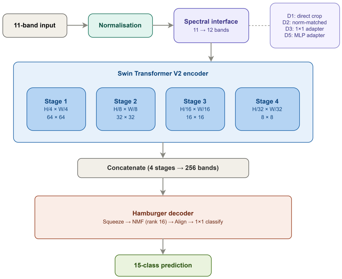
The segmentation model used in this study combines a pretrained Swin Transformer V2 encoder with a Hamburger decoder, following a standard encoder–decoder layout for dense prediction. The same decoder architecture is used in the MariNeXt baseline [20], enabling the direct comparison of encoder representations. Figure 1 illustrates the overall architecture and the position of the band adaptation within the processing pipeline.

3.3.1. Encoder: Swin Transformer V2

The encoder is a Swin Transformer V2 Base [21] initialised from the Hydro pretrained weights [7]. Its configuration is summarised in

Table 2. Swin Transformer V2 Base encoder configuration.

Parameter	Value
Embedding dimension	128
Stage depths	[2, 2, 18, 2]
Attention heads per stage	[4, 8, 16, 32]
Window size	16
Pretrained input bands	12
Target input bands	11

. The architecture consists of four hierarchical stages that produce feature maps at progressively reduced spatial resolutions (1/4, 1/8, 1/16, and 1/32 of the input). Each stage applies shifted window self-attention with a window size of 16 tokens. The patch embedding layer at the input projects the spectral bands into a 128-dimensional token space through a convolutional operation with kernel and stride of 4. In its pretrained form, this layer expects 12 input bands that correspond to the Sentinel-2 bands B01 through B12 (excluding B10). The adaptation of this layer to the 11-band MADOS input is the subject of the band adaptation experiments described in Section 3.4. The encoder contains approximately 87.9 million parameters.

3.3.2. Decoder: Hamburger

The decoder follows the Hamburger design introduced by [33], which applies non-negative matrix factorisation (NMF) as a global context aggregation mechanism. The same decoder architecture is used in MariNeXt [20]. Feature maps from all four encoder stages are resized to the spatial dimensions of the first stage (64 × 64 for the 256 × 256 padded input) using bilinear interpolation and then concatenated along the band dimension. A squeeze convolution reduces the concatenated representations to 256 bands. The resulting feature map is processed by the Hamburger module, which decomposes the spatial features into a low-rank basis and coefficient matrices through iterative NMF updates. The decomposition uses a rank of 16, with 6 iterations during training and 7 during evaluation. Group normalisation with 32 groups is applied throughout the decoder. A final 1 × 1 convolution produces per-pixel logits for the 15 output classes. The decoder contains approximately 694,000 parameters, bringing the total model size to approximately 88.6 million parameters.

3.3.3. Reference Baseline: MariNeXt

MariNeXt [20] serves as the from-scratch baseline. It replaces the Swin Transformer encoder with a MSCAN, a four-stage convolutional encoder that employs cascaded dilated convolutions with kernel sizes of 5, 7, 11, and 21 to capture multi-scale spatial context. The authors trained the MSCAN encoder end-to-end alongside the Hamburger decoder. Both MariNeXt and the Swin V2 hybrid feed all four encoder stages into the decoder. Neither discards the first-stage features. An inverse-logarithmic class weighting constant of $c$ = 1.02 is used in loss weighting.

In its published configuration, MariNeXt includes VSCP augmentation, EMA weight averaging with a decay of 0.999, and TTA via eight geometric transformations with majority voting. For controlled comparisons in this study, MariNeXt was retrained using the present training and evaluation pipelines without these enhancements.

3.4. Strategies for the Preprocessing Mismatch

Three aspects of the preprocessing mismatch issue are treated as experimental variables: the spectral band adaptation, the input normalisation, and the encoder transfer mode. Each addresses a different aspect of the mismatch characterised in Section 3.2.

• The spectral band adaptation handles the missing band.
• The input normalisation determines the statistical reference frame in which the encoder operates.
• The encoder transfer mode controls whether the pretrained weights are preserved, partially adapted, or fully retrained.

The following paragraphs describe the options considered for each aspect and the reasoning behind them.

The spectral band adaptation addresses the 12-to-11 band mismatch. The pretrained patch embedding layer is a convolution with weight tensor of shape ($C_{out}, 12, k, k$) with $k$ = 4 that projects the 12 input bands into a 128-dimensional token space. Two families of adaptation are considered. Direct weight adaptation modifies the weight tensor to operate on 11 bands, preserving the pretrained mapping for the shared bands and adding no parameters. Learnt input adapters leave the patch embedding unchanged and prepend a trainable module that maps the 11 input bands to the 12 bands as the patch embedding layer expects. The five strategies are compared in

Table 3. Spectral band adaptation variants for mapping the 12-band pretrained patch embedding onto the 11 available MADOS bands. All variants use a frozen Hydro encoder with MADOS normalisation.

Variant	Method	Parameters	Encoder
D1	Direct column crop	0	Frozen
D2	Crop + Frobenius rescaling	0	Frozen
D3	1 × 1 convolution (11-to-12)	144	Frozen
D4	D3 + partially unfrozen (ep. 40)	144	Partial
D5	MLP (11, 24, 11, GELU)	588	Frozen

.

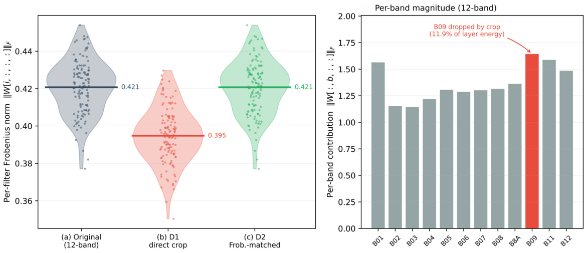
D1 (direct crop) removes the B09 column from the weight tensor without further modification. D2 (Frobenius-matched crop) removes the column and rescales each filter so that its Frobenius norm matches the original 12-band value. This compensates for the magnitude reduction caused by the lost dot-product term and preserves the activation configuration under which the downstream layer normalisation and self-attention blocks were optimised. D3 (linear adapter) prepends a 1 × 1 convolution from 11 to 12 bands, which is initialised so that the 11 shared bands pass through unchanged to their corresponding positions in the 12-band patch embedding, and the missing B09 band is seeded from the spectrally adjacent B8A band (detailed below). This adds 144 trainable parameters. D4 (adapter with partial unfreezing) extends D3 by unfreezing the last encoder stage at epoch 40 with a learning-rate scale of 0.05 times the decoder rate. D5 (nonlinear adapter) replaces the linear mapping with a two-layer perceptron with GELU activation and a hidden width of 24, as detailed below. The total parameter count is 588.

In particular, regarding variant D3, it uses a 1 × 1 convolution implemented as a linear projection from 11 input bands to 12 output bands, acting on the input band vector at each spatial location. The weight matrix is initialised so that each of the 11 MADOS bands passes through unchanged to its corresponding position in the 12-band patch embedding, and the missing B09 output band is initialised by copying the spectrally adjacent B8A band (864 nm and 945 nm). The bias vector is initialised to zero. The adapter contributes 144 trainable parameters (132 weight entries plus 12 biases), which are refined by a gradient descent during training.

In addition, the variant D5 replaces the linear projection with a two-layer perceptron. The first layer is a linear projection of ${\mathbb{R}}^{11}$ to ${\mathbb{R}}^{24}$ with bias, followed by GELU activation. The second layer is a linear projection of ${\mathbb{R}}^{24}$ to ${\mathbb{R}}^{12}$ with bias and no output activation. The parameter count is (11 × 24 $+$ 24) $+$ (24 × 12 $+$ 12) = 588. All parameters are trainable from random initialisation (Kaiming uniform for the linear weights, zero for the biases).

The input normalisation determines the per-band affine transformation applied to the raw reflectance values before they reach the band adaptation. Two competing objectives exist. The first is encoder compatibility: feeding the encoder inputs whose statistics match the pretraining dataset (Hydro z-score) preserves the operating configuration for which its weights were optimised. The second is decoder consistency: feeding the encoder inputs whose statistics match the downstream training set (MADOS z-score) ensures that the decoder learns representations under the same distribution it will encounter at test time. These two objectives conflict when the pretraining and downstream distributions differ (see Table 1).

The affine MADOS-to-Hydro (M2H) attempts to satisfy both objectives by mapping MADOS statistics onto Hydro statistics, though in practice this produces a third distribution that satisfies neither objective fully. The learnable affine strategy allows the network to discover the optimal mapping, but it may overfit with only 22 parameters and limited training data. The five strategies are compared and summarised in

Table 4. Normalisation strategies.

Strategy	Transformation	Parameters
MADOS z-score	${\displaystyle \frac{x-{\mu }_{MADOS}}{{\sigma }_{MADOS}}}$	Fixed (training set)
Hydro z-score	${\displaystyle \frac{x-{\mu }_{Hydro}}{{\sigma }_{Hydro}}}$	Fixed (pretraining)
Patch z-score	${\displaystyle \frac{x-{\mu }_{Patch}}{{\sigma }_{Patch}}}$	Per patch
Affine M2H	$\alpha x+\beta$, $\alpha ={\displaystyle \frac{{\sigma }_{Hydro}}{{\sigma }_{MADOS}}}$	Fixed (derived)
Learnable affine	$\alpha x+\beta$, optimised	22 trainable

.

The encoder transfer mode controls whether the pretrained weights are updated during training. With 1433 training patches and an encoder containing 87.9 million parameters, the ratio of supervised pixels to encoder parameters is low. Full fine-tuning in this configuration risks overwriting the general spectral and spatial features learnt during pretraining with noisy gradients derived from a small dataset. Freezing the encoder avoids this risk entirely. Only the 694,000-parameter decoder is trained. Partial unfreezing offers a middle ground: the encoder begins frozen, and only the last transformer stage becomes trainable after a specified number of epochs with a reduced learning rate. This limits the number of updated parameters and delays adaptation until the decoder has stabilised. The three modes are compared: frozen, partial unfrozen, and fully fine-tuned.

3.5. Analysis Methods

3.5.1. Feature-Space Separability

The primary source of classification errors in the MADOS task is the confusion between oil spill and Marine Water. In the published confusion matrix [20], 28.3% of oil spill test pixels are misclassified as Marine Water. To measure this effect, feature vectors are extracted at two points in the decoder: before the Hamburger NMF (pre-HAM) and after it (post-HAM). For each class, a centroid is computed as the mean feature vector over all annotated test pixels of that class. The cosine distance between oil spill and Marine Water centroids quantifies how well the decoder separates these two classes in its internal representation. Comparing this distance across normalisation strategies reveals whether the selection of input statistics affects the decoder’s ability to distinguish oil from water.

3.5.2. Band-Occlusion Attribution

To determine which spectral bands contribute most to each class prediction, a leave-one-out occlusion protocol is applied, following the permutation importance framework of [34] and the occlusion sensitivity analysis of [35], with per-class IoU as the scoring function. For each of the 11 bands in turn, all input values for each band are set to zero across the full test set, and the complete evaluation is repeated. The importance of band b for class c is defined as

$$I_{b,c}={IoU}_c-{IoU}_c^{(-b)}$$

(2)

where ${IoU}_c$ is the class IoU with all bands present, and ${IoU}_c^{(-b)}$ is the IoU when band b is set to zero. A positive value indicates that removing band b reduces segmentation accuracy for class c. Because inputs are normalised using MADOS per-band statistics, setting a band to zero in the network input corresponds to replacing the physical reflectance with the MADOS per-band mean.

The protocol is applied to matched pairs of normalisation strategies (B1 with MADOS z-score and B2 with Hydro z-score) using identical architecture and training. The shift in per-band importance between the two strategies is then correlated with the absolute normalised mean gap $\left|\delta \mu \right|$ from Table 1 using the Spearman rank coefficient, which measures monotonic associations without assuming linearity and is robust to outliers in the per-patch metric. A strong positive correlation would indicate that the bands most affected by the preprocessing mismatch are the same bands whose utilisation changes when the normalisation is switched.

3.5.3. Patch-Level Radiometric Analysis

To assess whether normalisation sensitivity varies across the test set, a patch-level analysis is conducted. For each of the 728 test patches, the spectral distance to the normalisation reference distribution is computed. Performance is evaluated twice for each patch: once with matched normalisation (the statistics used during training) and once with mismatched normalisation (the alternative set of statistics). The per-patch performance drop, defined as the matched-condition metric minus the mismatched-condition metric, is compared with the spectral distance using the Spearman rank coefficient. This analysis tests whether patches whose radiometric properties deviate more from the training-time reference undergo greater degradation under normalisation mismatch.

3.6. Experimental Protocol

3.6.1. Training Configuration

All experiments follow a common training configuration unless otherwise specified. The 11-band MADOS patches are loaded as per-band GeoTIFF files at their native spatial resolutions (10 m, 20 m, 60 m), upsampled to a common 10 m grid via nearest-neighbour interpolation, and stacked into tensors of shape (11, 240, 240). Pixels containing missing values (NaN) are replaced with per-band global means derived from the MADOS training set [20]. Normalisation is then applied according to the strategy under evaluation (Section 3.4). Finally, images are centre-padded to 256 × 256 using the constant zero fill to match the Hydro encoder expected input dimensions. The corresponding mask positions are filled with $-$1 so that padded pixels are excluded from the loss and all other evaluation metrics. The padded border is visible to the encoder during the forward pass and contributes to spatial context, but it does not generate supervised gradients or affect reported scores.

Models are trained for 80 epochs using the Adam optimiser with an initial learning rate of 2 × 10⁻⁴ and no weight decay. A multistep schedule reduces the learning rate by a factor of 10 at epochs 45 and 65. The batch size is 5. The loss function is the cross-entropy with inverse-logarithmic class weighting, which is computed as

$$w_i={\displaystyle \frac{1}{\mathrm{l}\mathrm{o}\mathrm{g}(c+p_i)}}$$

(3)

where $p_i$ is the pixel fraction of class $i$ in the training set and $c$= 1.02. No label smoothing is applied.

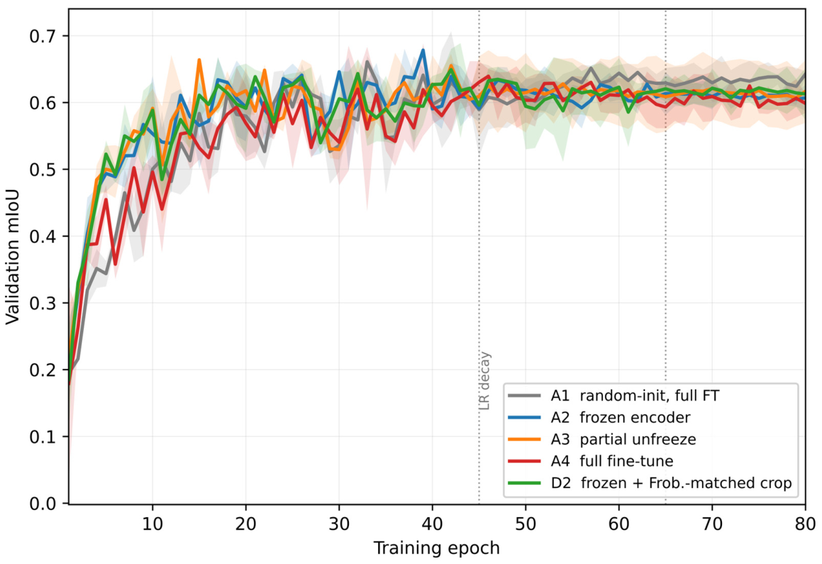
Data augmentation in the controlled blocks consists of random horizontal flips, random vertical flips, and random rotations (90°, 180°, or 270°) applied with 80% probability. VSCP augmentation [20], EMA, and TTA are all disabled in the controlled blocks. Model selection retains the checkpoint with the highest validation mIoU across the 80-epoch run. The last-epoch checkpoint is also stored but is not used for test evaluation in the controlled blocks. Validation mIoU trajectories across the 80-epoch experiments are provided in Appendix E. Each configuration is trained with two random seeds (0 and 1). These seeds control the weight initialisation, data loader shuffling, and augmentation randomness. The results are reported as the mean and standard deviation over seeds. The limited number of seeds is a constraint imposed by the available compute and is acknowledged in Section 5.7.

3.6.2. Encoder Transfer Mode Settings

In the frozen configuration, all encoder parameters are set to evaluation mode and receive no gradients. In the fully fine-tuned configuration, all parameters are trainable from epoch 1 at the same learning rate. In the partially unfrozen configuration, the encoder begins frozen, and the last $k$ stages become trainable at a specified epoch. The encoder learning rate is scaled relative to the decoder rate. The specific settings vary by block. Block A3 uses a scale of 0.10, with the last stage unfrozen from epoch 1. Block D4 uses a scale of 0.05, with the last stage unfrozen from epoch 40. The bridge ablation configurations use a scale of 0.10, with the last stage unfrozen from epoch 1. Throughout this work, partial unfreezing denotes any configuration in which the last k encoder stages become trainable while the remainder stay frozen. As such, each configuration is specified by three quantities: the number of unfrozen stages, the epoch from which they are trainable, and the encoder learning-rate scale relative to the decoder. No separate term is used for configurations whose unfreezing is delayed, as the epoch parameter carries this information. The partially unfrozen blocks (P1 through P4) use a scale of 0.05, with the last stage unfrozen at epoch 40 (P1, P2, P4) or epoch 25 (P3).

3.6.3. Controlled Block Configurations

The experiments in this study are organised into six groups, referred to here as experimental blocks, each of which isolates a single variable while holding all others fixed. Each block is a set of training or evaluation runs. The term “block” denotes an experimental grouping and is unrelated to the transformer blocks of the encoder architecture. The six blocks are: block A (encoder transfer mode), block B (input normalisation strategy), block C (test-time perturbation robustness), block D (spectral band adaptation), block H (label-free harmonisation), and block P (augmented training extension framework). Within each block, individual configurations are identified by the block letter and an index. For example, A2 denotes the second configuration of block A. The band adaptation configurations of D1–D5 introduced in Section 3.4 correspond to the rows of block D.

Table 5. (a) Controlled block configurations for blocks A, B, and D. All blocks use the Hamburger decoder, 80 epochs, Adam optimiser, $c$ = 1.02, no VSCP, no EMA, and no TTA. (b) Block C perturbation conditions. All applied to the B1 checkpoint at test time. (c) Block H label-free harmonisation transforms. All applied to the B1 checkpoint at test time. (d) Extension framework configurations. All use the Hydro encoder. Frozen mirror rows duplicate the settings of their partially unfrozen counterpart (same seeds, epochs, learning rate schedule, VSCP, EMA, and TTA), differing only in that the encoder remains frozen throughout training. This paired design isolates the contribution of encoder unfreezing from the contribution of the augmented training configuration.

(a)
Configuration	Block	Encoder Initialisation	Transfer Mode	Normalisation	Adapter
A1	A	Random	Full	MADOS	None
A2	A	Hydro	Frozen	MADOS	None
A3	A	Hydro	Partial (last stage = 1, ep. 1, lr × 0.10)	MADOS	None
A4	A	Hydro	Full	MADOS	None
B1	B	Hydro	Frozen	MADOS z-score	None
B2	B	Hydro	Frozen	Hydro z-score	None
B3	B	Hydro	Frozen	Patch z-score	None
B4	B	Hydro	Frozen	Affine M2H	None
B5	B	Hydro	Frozen	Learnable affine	None
D1	D	Hydro	Frozen	MADOS	Direct crop
D2	D	Hydro	Frozen	MADOS	Frobenius-matched crop
D3	D	Hydro	Frozen	MADOS	1 × 1 adapter
D4	D	Hydro	Partial (last stage = 1, ep. 40, lr × 0.05)	MADOS	1 × 1 adapter
D5	D	Hydro	Frozen	MADOS	MLP adapter
(b)
Condition		Perturbation		Operational Analogue
C1 (clean)		None (reference)		-
C2 (gain 0.95)		All bands × 0.95		Sensor calibration drift
C2 (gain 1.05)		All bands × 1.05		Atmospheric transmittance shift
C3 (bias −0.005)		All bands − 0.005		Dark current offset
C3 (bias +0.005)		All bands + 0.005		Path radiance increase
C4 (noise)		Gaussian, $\sigma$ = 0.005		Detector noise
C5 (wrong normalisation)		Hydro stats at test time		Different atmospheric correction pipeline
C6 (reverse normalisation)		MADOS stats at test time, model trained under Hydro stats		Reverse-direction normalisation mismatch
(c)
Transform		Description		Reference Distribution
H1		Robust per-band percentile stretch (2–98%) + post-clip re-standardisation		MADOS train split
H2		Diagonal CORAL: per-band rescaling ${\displaystyle \frac{{\sigma }_{Hydro}}{{\sigma }_{MADOS}}}$, re-centring to ${\mu }_{Hydro}$		Hydro pretraining statistics
H3		Per-patch affine to Hydro median/IQR (gain bounded to [0.8, 1.2])		Hydro pretraining statistics
(d)
Configuration	Transfer Mode	Normalisation	Adaptation	VSCP	EMA	TTA
D2 ceiling	Frozen	MADOS	D2	On	0.999	On
P1	Partial (ep. 40, lr × 0.05)	Hydro	D3	On	0.999	On
P1 frozen mirror	Frozen	Hydro	D3	On	0.999	On
P2	Partial (ep. 40, lr × 0.05)	MADOS	D2	On	0.999	On
P2 frozen mirror	Frozen	MADOS	D2	On	0.999	On
P3	Partial (ep. 25, lr × 0.05)	Hydro	D3	On	0.999	On
P3 frozen mirror	Frozen	Hydro	D3	On	0.999	On
P4	Partial (ep. 40, lr × 0.05)	Hydro	D3	On	Off	Off
P4 frozen mirror	Frozen	Hydro	D3	On	Off	Off

a specifies the configurations for blocks A, B, and D. Block C and block H configurations are reported in Table 5b and Table 5c, respectively.

Block A evaluates the four encoder transfer modes (random initialisation with full training, Hydro with full fine-tuning, partial unfreezing, and frozen encoder), all using MADOS normalisation with no spectral adapter. Block B compares the five normalisation strategies with a frozen Hydro encoder and no adapter. Block D compares the five band adaptation strategies with a frozen Hydro encoder and MADOS normalisation. Block C evaluates the B1 checkpoint under six perturbation conditions at the test time without additional training. These perturbations simulate operational scenarios: multiplicative gain simulates sensor calibration drift or atmospheric transmittance variation, additive bias simulates path radiance offset, Gaussian noise simulates detector noise, and wrong normalisation simulates deployment on data processed through a different atmospheric correction pipeline.

Block H evaluates three label-free harmonisation transforms as candidate mitigations for the normalisation mismatch identified in Block C. Each row of block H trains a model from scratch on the D2 architecture, with the harmoniser substituted for the per-band MADOS z-score in the input pipeline. The four rows of block H (baseline plus H1, H2, and H3) differ only in this input normalisation. Each harmoniser is fitted from the MADOS training split (H1, H2) or on a per-scene basis at inference (H3) and requires no access to target-class labels. H1 performs a per-band 2nd–98th percentile stretch followed by an additive re-standardisation using the post-clip mean and standard deviation. H2 applies a diagonal CORAL alignment in which each band is rescaled by the ratio of the Hydro-to-MADOS standard deviations and re-centred to the Hydro mean, producing an output in the raw Hydro reflectance space that the encoder was pretrained on. H3 replaces the dataset’s global gain and bias of H2 with a per-scene calibration, in which the scene median and interquartile range (IQR) are matched to the Hydro target statistics, with the multiplicative gain bounded to [0.8, 1.2] and the additive bias bounded to ±0.25 times the target IQR to prevent overcorrection on patches dominated by a single material. Full specifications of H1, H2, and H3 are given in Appendix C.

3.6.4. Extension Frameworks

The extension frameworks depart from the controlled setup to quantify the contributions of individual training enhancements. Table 5d specifies each extension’s configuration.

The ceiling framework trains D2 using VSCP and EMA (decay 0.999) with the encoder frozen, as evaluated with TTA. The partially unfrozen sweep (P1 through P4) combines partial unfreezing with VSCP. P1 through P3 additionally enable EMA and TTA. P4 serves as a no-EMA and no-TTA control. VSCP operates within each training batch by replacing annotated pixels from one image with annotated pixels from another, synthesising additional training samples without external data [20]. TTA applies eight geometric transformations (four rotations combined with horizontal flipping) and aggregates predictions by majority voting.

For each partially unfrozen configuration, a frozen mirror counterpart is trained with identical settings (same seeds, epochs, learning rate schedule, augmentation, EMA, TTA). The only difference is that the encoder remains frozen throughout. This paired design isolates the contribution of encoder unfreezing from the effect of the augmented training configuration.

3.6.5. Evaluation

Evaluation is performed at the pixel level on the 728-patch test set. During inference, the model produces logits at the decoder output resolution, which are cropped to the original 240 × 240 pixel size. Class predictions are obtained through the argmax over the band dimension. Only pixels with valid ground-truth labels (label ≠ $-1$) contribute to the metrics. Padded border pixels and unannotated regions are excluded. Three primary metrics are reported: mean Intersection over Union (mIoU), macro-averaged F1 score (macro F1), and overall accuracy (OA). Inference in this implementation is not deterministic by default, as the LightHam decoder head initialises its non-negative matrix factorisation bases randomly at each forward pass, so repeated evaluations of a single checkpoint yield slightly different predictions unless the random-number stream is fixed. All results reported here were produced with a fixed evaluation seed, unit batch size and fixed dataset ordering; under this protocol every configuration reproduces its reported mIoU exactly. Reported cross-seed standard deviations therefore reflect training stochasticity alone. All configurations are trained with two random seeds (0 and 1). This reflects a deliberate allocation of a fixed compute budget: the full experimental programme comprises 92 training runs across six controlled blocks, and seed replication was traded against coverage of the preprocessing factor space. Cross-seed standard deviations are reported throughout, and differences smaller than the relevant standard deviation are reported as indistinguishable rather than as clear rankings. Because test patches drawn from the same Sentinel-2 scene are not independent, uncertainty attributable to test-set sampling is estimated by a scene-level bootstrap: the 42 test scenes are resampled with replacement over 10,000 iterations, per-scene confusion matrices are summed within each resample, and mIoU is recomputed under the reduction defined above. Intervals are reported for the mean-over-seed statistic used throughout the manuscript. The results are given in Appendix H.

3.6.6. Computational Resources

Training and evaluation were conducted on a workstation equipped with an NVIDIA GeForce RTX 4060 Ti GPU, using CUDA 12.4 and PyTorch 2.5.1 under Python 3.10. A single 80-epoch training run requires approximately 1 h for frozen encoder configurations and approximately 2 h for full fine-tuning. All metrics are computed using scikit-learn 1.6.0 and pooled across the full test set.

4. Results

4.1. Transfer Strategy

Table 6. Transfer strategy comparison. P1 frozen mirror uses VSCP, EMA, and TTA with a frozen encoder and D3 adapter under Hydro normalisation. Bold marks the best value per column. MariNeXt (ctrl) refers to the experiment without the training enhancements and retrained with the present settings.

Configuration	Encoder	Transfer Mode	mIoU	$\mathit{\sigma }$	Macro F1	Overall Accuracy
A4	Hydro	Full fine-tune	0.489	0.037	0.618	0.833
A1	Random	Full (scratch)	0.528	0.030	0.652	0.850
A3	Hydro	Partial	0.540	0.022	0.649	0.855
MariNeXt (ctrl)	MSCAN	Full (scratch)	0.559	-	0.684	0.896
A2	Hydro	Frozen	0.574	0.005	0.699	0.838
D2	Hydro	Frozen + D2	0.600	0.004	0.726	0.858
MariNeXt [20]	MSCAN	Full (scratch)	0.643	-	0.760	0.891
P1 frozen mirror	Hydro	Frozen + D3	0.660	0.024	0.772	0.867

summarises the results for block A, which compares four encoder transfer modes, together with the D2 band adaptation configuration and the MariNeXt baseline. Among the Hydro-initialised configurations, the frozen encoder (A2) achieves the highest mIoU at 0.574, followed by partial unfreezing (A3, 0.540) and full fine-tuning (A4, 0.489). The full fine-tuned Hydro encoder performs worse than a randomly initialised encoder trained from scratch (A1, 0.527). The frozen configuration also exhibits the lowest inter-seed variance ($\sigma$ = 0.005).

Adding the D2 band adaptation (Frobenius-matched weight crop) to the frozen encoder raises performance to 0.600 mIoU, which exceeds the MariNeXt baseline retrained in the present codebase without training enhancements (0.559 mIoU) by 4.1%. When engineering enhancements are enabled, the frozen Hydro encoder (P1 frozen mirror, 0.660 mIoU with VSCP, EMA, and TTA) reaches a mean mIoU 1.7% above the published MariNeXt result (0.643 mIoU with VSCP, EMA, and TTA). Given $\sigma$ = 0.024 for P1 frozen mirror, the matched comparison falls within seed variability ($\Delta$ = 0.017 < $\sigma$). The two configurations are therefore reported as a match rather than as an improvement of one over another. It is also noted that the published MariNeXt achieves the highest overall accuracy (0.891) in Table 6, while the frozen Hydro configurations achieve the highest mIoU and macro F1. This pattern is expected on a heavily imbalanced dataset. A classifier that performs slightly better on the dominant water classes can score higher on the pixel-pooled overall accuracy, while macro-averaged mIoU and F1, which weight all classes equally, favour configurations that improve on the minority classes.

To verify whether the gains observed in the extension frameworks originate from encoder unfreezing or from the augmented training techniques, two complementary comparisons were performed: a bridge ablation between matched frozen and partially unfrozen configurations under controlled conditions (no VSCP, EMA, and TTA), and a frozen mirror set under the augmented recipe (VSCP, EMA, and TTA enabled). Three matched bridge ablation pairs are derivable from the controlled blocks: A2 (frozen, no adapter) versus A3 (partial unfreezing from epoch 1, no adapter); D2 (frozen, Frobenius-matched crop) versus D4 (partial unfreezing from epoch 40, D3 adapter); and D3 (frozen, D3 adapter) versus D4 (partial unfreezing from epoch 40, D3 adapter). In all three pairs, the frozen configuration outperforms the partially unfrozen counterpart: A2 (0.574)—A3 (0.540) = +0.034; D2 (0.600)—D4 (0.575) = +0.025; D3 (0.582)—D4 (0.575) = +0.006. The first two differences exceed the cross-seed standard deviation of the partially unfrozen variant ($\sigma$ = 0.022 for A3, $\sigma$ = 0.033 for D4) and are therefore robust. The third is within seed variability. In the frozen mirror experiments, the same training conditions were applied (including VSCP, EMA, and TTA) with and without encoder unfreezing. Across the four matched extension framework pairs, the frozen mirror clearly exceeds the partially unfrozen counterpart in two cases (P2: 0.611 versus 0.590, $\Delta$ = +0.022; P4: 0.620 versus 0.593, $\Delta$ = +0.027). In the remaining two cases, the direction is reversed: P1 partial (0.663) marginally beats P1 frozen mirror (0.660) by $\Delta$ = +0.003, well within the frozen mirror standard deviation of $\sigma$ = 0.024; and P3 partial (0.662) beats P3 frozen mirror (0.631) by $\Delta$ = +0.031, comparable to the partially unfrozen standard deviation of $\sigma$ = 0.048. Across all four pairs, partial unfreezing produces no statistically robust gain over frozen encoder training under matched VSCP + EMA + TTA conditions: when partial wins, the margin is within seed variability, whereas when frozen mirror wins, the margins (0.022 and 0.027) are larger than typical seed dispersion. The frozen encoder configuration is therefore as good as or better than the partially unfrozen one in every pair tested modulo cross-seed noise.

4.2. Band Adaptation

Table 7. Band adaptation comparison. All bands use the frozen Hydro encoder with MADOS normalisation. Bold marks the best value per column.

Variant	Method	Parameters	mIoU	$\mathit{\sigma }$
D1	Direct column crop	0	0.553	0.034
D2	Crop + Frobenius rescaling	0	0.600	0.004
D3	1 × 1 convolution (11-to-12)	144	0.582	0.043
D4	D3 + partial unfreeze	144	0.575	0.033
D5	MLP (11, 24, 12)	588	0.509	0.038

presents the results for block D, which compares five strategies for adapting the 12-band pretrained patch embeddings to the 11 MADOS bands. All configurations use a frozen encoder with MADOS normalisation.

The Frobenius-matched crop (D2) achieves the highest mean mIoU (0.600) and the lowest cross-seed deviation (0.004). The direct crop without rescaling (D1) reaches 0.553, indicating that the Frobenius norm compensation in D2 accounts for a gain of 4.7%. The learnt linear adapter (D3) reaches 0.582 with substantially higher variance ($\sigma$ = 0.043). Adding partial encoder unfreezing from epoch 40 (D4, 0.575) does not improve over D3 and increases instability. The nonlinear MLP adapter (D5) yields the lowest performance across all variants (0.509). Across the five strategies, the zero-parameter weight adaptation (D2) attains the highest mean mIoU and the lowest cross-seed dispersion. Its margin over the learnt linear adapter (D3, Δ = 0.018) falls within D3’s inter-seed variability, so D3 cannot be declared inferior in mean; thus, the comparison establishes that the learnt adapter delivers no demonstrable benefit over the zero-parameter alternative while introducing 144 trainable parameters and markedly higher run-to-run variance. Against the direct crop (D1, Δ = 0.047) and the MLP adapter (D5, Δ = 0.091), the advantage of D2 exceeds inter-seed variability. A paired scene-level bootstrap over the 42 test scenes places the D2—D3 difference at +0.019 with a 95% interval of [−0.012, +0.052]; the sign is preserved in 89% of resamples, so the ordering is directionally consistent but not resolvable against scene-level sampling noise.

4.3. Normalisation

4.3.1. Matched Normalisation

Table 8. Normalisation strategy comparison. All strategies use the frozen Hydro encoder without spectral adapter. Bold marks the best value per column.

Configuration	Strategy	mIoU	$\mathit{\sigma }$
B1	MADOS z-score	0.571	0.016
B2	Hydro z-score	0.560	0.027
B3	Patch z-score	0.478	0.026
B4	Affine M2H	0.404	0.007
B5	Learnable affine	0.386	0.003

reports the results for block B, in which the five normalisation strategies are compared using a frozen Hydro encoder without a spectral adapter.

The MADOS z-score (B1, 0.571) and Hydro z-score (B2, 0.560) both yield higher mIoU than the remaining alternatives. A paired scene-level bootstrap resampling the 42 test scenes gives a difference of +0.011 with a 95% interval of [−0.019, +0.081]. The sign is preserved in 82% of resamples whereas the interval includes zero. The difference between B1 and B2 is small (0.011 mIoU) and falls within the range of inter-seed variability for B2 ($\sigma$ = 0.027). MADOS normalisation is marginally preferred for this task. Patch z-score (B3, 0.478) performs worse. The per-patch statistics are noisy and vary with scene composition, resulting in inconsistent input distributions across the training and test samples. The explicit domain alignment strategies, affine M2H (B4, 0.404) and learnable affine (B5, 0.386), yield the lowest accuracy. Although designed to reduce distributional divergence, they produce a synthetic distribution that matches neither dataset. The encoder performs best when it receives globally consistent statistics from either reference rather than a statistical compromise.

4.3.2. Normalisation Mismatch

Table 9. Block C perturbation robustness. $\Delta$ denotes change relative to the clean condition.

Configuration	mIoU	$\mathit{\Delta }$
Clean	0.571	-
Gain 0.95	0.588	+0.017
Gain 1.05	0.550	−0.021
Bias −0.005	0.574	+0.004
Bias +0.005	0.547	−0.024
Noise $\sigma$ = 0.005	0.507	−0.064
Wrong normalisation (Hydro)	0.113	−0.458
B2 clean (Hydro normalisation)	0.560	-
C6 reverse (MADOS stats at test)	0.241	−0.319

reports the perturbation robustness results from block C. The B1 checkpoint (frozen encoder, MADOS normalisation) was evaluated under six perturbation conditions applied to the test inputs, without additional training.

Multiplicative gain perturbations of ±5% produce mIoU changes of +0.017 (gain = 0.95) and −0.021 (gain = 1.05). Additive bias perturbations of ±0.005 produce changes of +0.004 and −0.024. Gaussian noise ($\sigma$ = 0.005) reduces mIoU by 0.064. Applying the wrong normalisation statistics (Hydro z-score applied to a model trained with MADOS z-score) reduces mIoU from 0.571 to 0.113. This degradation is an order of magnitude larger than any of the radiometric perturbations tested.

The reverse direction was evaluated to establish whether this collapse depends on which set of statistics is substituted. The B2 checkpoint, trained under Hydro statistics, was evaluated on the same test data with MADOS statistics applied at inference (C6). That is, performance falls from 0.560 to 0.241 mIoU, a loss of 0.319, with overall accuracy declining from 0.858 to 0.661 and macro F1 from 0.674 to 0.327. Mismatched normalisation is therefore catastrophic in either direction, and the effect reported above is not an artefact of the direction tested. The magnitudes are not equal, as the forward direction loses 80.2% of its clean mIoU against 57.0% in the reverse at a ratio of 0.70. Per-class behaviour is correspondingly uneven. Under C6, Oil Platform loses 0.68 IoU, Jellyfish 0.50 (to exactly zero), turbid water 0.46, and foam 0.44, whereas Marine Water loses 0.16 and Sediment-Laden Water 0.21. The rare classes that the Hydro-normalised pipeline recovers are also the first to disappear when the normalisation is mismatched.

Table 10. Block H label-free harmonisation transforms. Each row trains a model from scratch on the D2 architecture with the harmoniser substituted for MADOS z-score. The baseline retains MADOS z-score. Values are mean mIoU across two seeds. Bold marks the best value in the column.

Transform	mIoU	$\mathit{\sigma }$
Baseline (no transform)	0.566	0.029
H1 (percentile + re-standardisation)	0.514	0.003
H2 (diagonal CORAL)	0.409	0.010
H3 (per-patch affine)	0.345	0.008

reports the block H results, in which three label-free harmonisation transforms are evaluated as candidate mitigations for the normalisation mismatch revealed in block C. Each row was trained from scratch on the D2 architecture with the harmoniser substituted for MADOS z-score. The baseline row uses the same architecture with MADOS z-score retained. None of the three transforms recovers the matched normalisation performance: H1 (percentile stretch with post-clip re-standardisation) reaches 0.514, H2 (diagonal CORAL alignment to Hydro reflectance) reaches 0.409, and H3 (constrained per-patch affine to Hydro) reaches 0.345 mIoU. All three fall below the D2 configuration (0.600) and below the unmodified MADOS z-score baseline of this block (0.566). The relative ordering baseline > H1 > H2 > H3 is preserved across the two seeds.

4.4. Mechanism: Normalisation Controls Band Utilisation

The results in the preceding sections indicate that MADOS and Hydro normalisation produce similar aggregate performance (0.571 versus 0.560) while the mismatch at test time is catastrophic. This section examines the internal mechanism through which normalisation affects the pretrained encoder.

4.4.1. Feature-Space Separability

Table 11. Decoder feature-space separability of oil spill versus Marine Water class centroids, measured cosine distance.

Configuration	Normalisation	Hook	Cosine Distance
B1	MADOS	pre-HAM	0.079
B2	Hydro	pre-HAM	0.117
D2	MADOS	pre-HAM	0.092
B1	MADOS	post-HAM	0.194
B2	Hydro	post-HAM	0.388
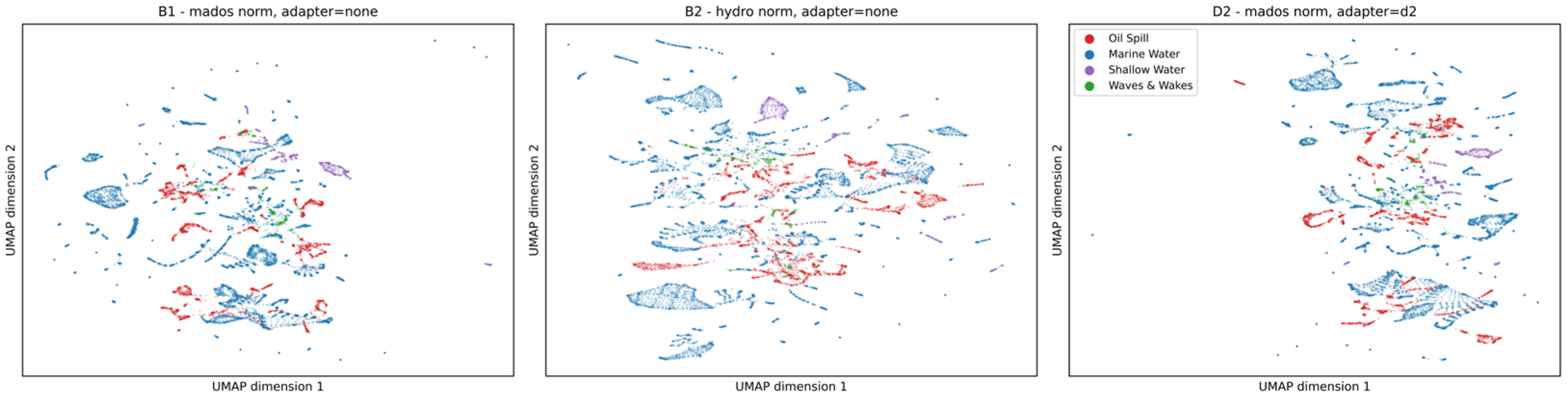
D2	MADOS	post-HAM	0.252

reports the cosine distance between oil spill and Marine Water class centroids in the decoder feature space, measured at two hook points. Under MADOS normalisation (B1), the pre-Hamburger (pre-HAM) cosine distance between the two classes is 0.079. Under Hydro normalisation (B2), this increases to 0.117, representing a factor of 1.5. After the Hamburger NMF module, the separation grows from 0.194 (B1) to 0.388 (B2) at a factor of 2.0. The NMF module amplifies the normalisation-induced separability advantage: the ratio of post-Hamburger (post-HAM) to pre-HAM distance is 2.5 under MADOS normalisation and 3.3 under Hydro normalisation. Figure 2 shows the corresponding UMAP projection of the pre-HAM decoder features for the B1, B2, and D2 configurations.

These measurements indicate that, although the aggregate mIoU difference between B1 and B2 is only 0.011, the decoder’s internal geometry for the oil spill versus Marine Water boundary differs substantially. Hydro normalisation produces a feature space in which the two most confused classes are better separated, when this advantage is diluted in the 15-class macro-averaged metric.

4.4.2. Band-Occlusion Attribution

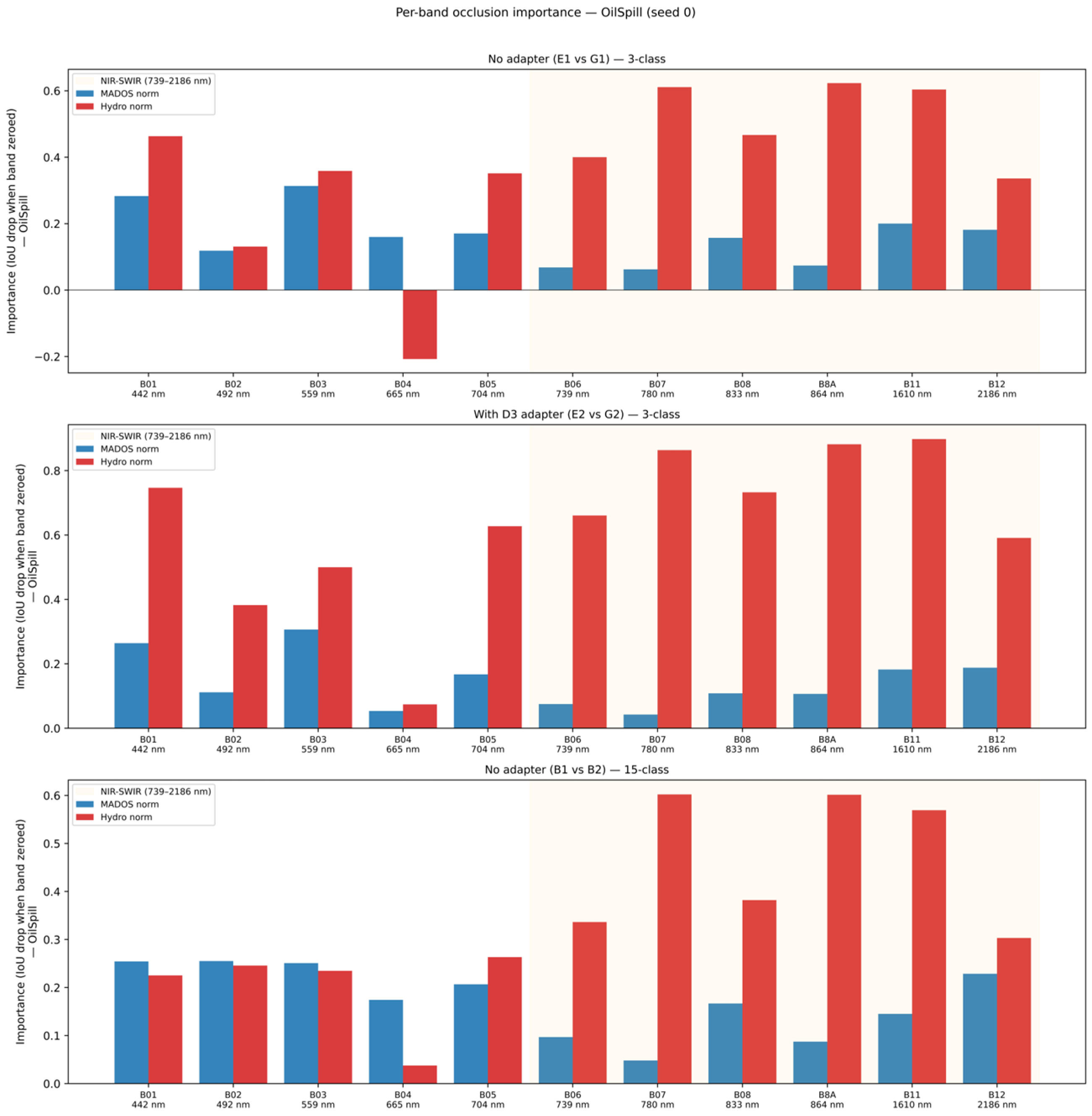
To determine whether the separability difference reflects a change in spectral band utilisation, a band-occlusion analysis was conducted on the B1 versus B2 pair. Figure 3 shows the per-band importance for oil spill under both normalisation strategies.

Under MADOS normalisation (B1), oil spill importance is distributed relatively evenly across all 11 bands, with the highest values in the visible range (B01 through B04) and moderate contributions from the near-infrared and shortwave infrared bands B06 (739 nm), B07 (780 nm), B8A (864 nm), and B11 (1610 nm). These are spectral regions where oil films modify the Fresnel surface through capillary wave damping [17] and where the SWIR bands bracket the diagnostic C-H stretch hydrocarbon absorption features near 1730 nm and 2300 nm [36]. Simultaneously, the importance of the red band (B04, 665 nm) decreases, indicating that the model reduces its reliance on a spectrally less diagnostic wavelength.

Table 12. Spearman rank correlation between the per-band importance shift under mismatched normalisation and the absolute normalised per-band mean gap between the MADOS and Hydro distributions.

Class	Spearman $\mathit{\rho }$	$\mathit{p}$-Value
Oil Spill	0.836	0.001
Marine Water	0.791	0.004

reports the Spearman rank correlation between the per-band importance shift (Hydro minus MADOS importance) and the absolute normalised mean gap $\left|\delta \mu \right|$ from Table 1. For oil spill, the correlation is 0.836 ($p$ = 0.001). For Marine Water, it is 0.791 ($p$ = 0.004). These values confirm that the bands most affected by the preprocessing mismatch are the same bands whose utilisation changes most when the normalisation is switched.

4.5. Spatial Structure of Normalisation Fragility

The normalisation mismatch effect reported in Section 4.3.2 represents an aggregate over all 728 test patches. To assess whether the degradation varies spatially, a patch-level analysis was conducted for the D2 configuration. For each test patch, the mIoU was evaluated under both matched (MADOS) and mismatched (Hydro) normalisation, and the drop was correlated with the spectral distance of that patch to the MADOS reference distribution.

Table 13. Patch-level Spearman correlations between spectral distance to the MADOS reference and the mIoU drop under mismatched normalisation (D2 configuration, marine patches, $n$ = 669).

Distance Metric	Spearman $\mathit{\rho }$	$\mathit{p}$-Value
$D_{MADOS}$ (Euclidean)	0.105	0.007
SAM-to-MADOS	0.080	0.038
$\Delta$ Mahalanobis	−0.088	0.022

reports the Spearman correlation for the marine patch subset (n = 669), which excludes patches dominated by land cover or coastal features. A positive correlation between the Euclidean distance to the MADOS reference mean ($D_{MADOS}$) and the mIoU drop is observed ($\rho$ = 0.105, $p$ = 0.007), indicating that patches whose spectral statistics deviate more from the MADOS training distribution experience greater degradation under mismatched normalisation, though the effect size is small. The spectral angle to the MADOS reference (SAM-to-MADOS) shows a similar trend ($\rho$ = 0.080, $p$ = 0.038), again with a small effect magnitude. The Mahalanobis distance shows the opposite sign ($\rho$ = −0.088, $p$ = 0.022). Mahalanobis whitens by the inverse MADOS covariance and therefore emphasises deviations along low-variance directions of the training distribution, whereas the failure mode under mismatched normalisation is driven by the systematic per-band mean offset between MADOS and Hydro, which is largely orthogonal to those low-variance directions. The three distance metrics therefore identify partially disjoint subsets of at-risk patches, with small effect sizes across the board, indicating that input radiometric statistics alone are weakly predictive of patch-level susceptibility to normalisation mismatch.

Unsupervised clustering of the test patches based on 28 radiometric descriptors (per-band medians, interquartile ranges, spectral indices, and water-pixel fractions) identifies two latent radiometric configurations within the marine partition ($k$ = 2, silhouette coefficient = 0.67). These clusters correspond to patches with different brightness profiles and water composition, indicating that MADOS is not radiometrically homogenous.

5. Discussion

5.1. Preprocessing Mismatch as the Dominant Factor in Transfer Performance

Across all controlled blocks, the configurations that most strongly affect performance are those that alter the statistical relationship between the input distribution and the encoder’s pretrained operating configuration. Block C demonstrates this most directly, as applying the wrong normalisation statistics at test time reduces mIoU by 0.458, roughly an order of magnitude larger than the largest radiometric perturbation tested. This dominance of normalisation over other preprocessing perturbations indicates that the encoder’s representations are tightly bound to the statistical distribution under which they were learnt, and that recovery from a mismatched distribution does not occur within the downstream layers.

Two observations support the framing of preprocessing mismatch as a transfer-level problem rather than a per-pixel calibration problem. First, the explicit domain alignment strategies (B4, B5) underperform in contrast to the simple z-score strategies (B1, B2). The encoder benefits from globally consistent statistics from either reference distribution, but not from a synthesised intermediate distribution that satisfies neither. Second, the label-free harmonisation transforms in block H (H1, H2, H3) also fall below B1, indicating that purely statistical alignment of source-to-target distributions is insufficient when the encoder’s internal feature distribution is the actual referent. None of the three block H transforms recovers the matched normalisation performance, even though all three reduce the marginal distance between source and target band statistics by design.

A distinction should be drawn between the preprocessing discrepancy documented in Section 3.1 and the mechanism established in block C. Hydro and MADOS differ in their atmospheric correction algorithm and reflectance convention, but they also differ in scene composition, geographic and temporal sampling, class definitions, and label distribution. The present design does not separate these sources, and the degradation reported here is therefore not attributed to atmospheric correction as such. What block C establishes is narrower and does not depend on that attribution, whereby holding the model, the imagery, and the labels as fixed and altering only the normalisation statistics applied at inference reproduces a collapse of 0.458 mIoU. The operative variable is the statistical correspondence between the input and the encoder’s pretrained operating point, irrespective of what produced the discrepancy. Isolating the contribution of atmospheric correction specifically would require the same imagery processed through several correction algorithms and evaluated under an otherwise identical protocol; this is identified as a direction for future work in Section 6.

5.2. Why Direct Weight Adaptation Outperforms Learnt Adapters

The band adaptation results in block D show that the zero-parameter Frobenius-matched crop (D2) exceeds the direct crop (D1) and the nonlinear MLP adapter (D5) by margins larger than inter-seed variability, and matches the learnt linear adapter (D3) at a tenth of its cross-seed dispersion and at zero-parameter cost. Two factors plausibly drive this. First, D2 preserves the exact pretrained mapping for the eleven shared bands and applied a closed-form magnitude correction. It introduces no degrees of freedom that can drift during training. Second, the learnt adapters operate before a frozen encoder whose weights were optimised under the original input configuration. Gradients flowing into the adapter must compensate not only for the missing band but also for any deviation between the encoder’s expected input geometry and the adapter’s output. With 144 (D3) or 588 (D5) parameters, this is a fragile optimisation, and the elevated cross-seed variance for D3 and D5 ($\sigma$ = 0.034 to 0.043) is consistent with this interpretation.

The 4.7% gain of D2 over D1 isolates the magnitude-compensation effect specifically. Removing one input band without rescaling reduces the per-filter dot-product magnitude by approximately one twelfth, which propagates as a distributional shift through the subsequent layer normalisation and self-attention blocks. The encoder’s downstream layers were not optimised under this shifted setting. The Frobenius rescaling in D2 restores the per-filter weight norm to the original 12-band value, eliminating this shift. The result is consistent with prior observations that activation-scale preservation matters when modifying the input layer of a pretrained network [14,29]. The distribution of per-filter Frobenius norms before and after this rescaling is reported in Appendix F.

5.3. Encoder Freezing Under Limited Target Data

The ratio of supervised pixels to encoder parameters in this transfer setting is low: 1433 training patches against an 87.9-million-parameter encoder. Under these conditions, full fine-tuning of the pretrained encoder (A4, 0.489 mIoU) underperforms not only with the frozen encoder (A2, 0.574) but also with a randomly initialised encoder trained from scratch (A1, 0.527). The from-scratch random model carries no prior assumptions about its representations and is therefore not at risk of overwriting useful structures. However, the fully fine-tuned pretrained model is. This pattern is consistent with the framing in Section 3.4.

The bridge ablation and frozen mirror experiments further indicate that the performance gains in the extension frameworks (P1–P4) originate from the augmented training setting (VSCP, EMA, TTA) rather than from encoder unfreezing. Across the four matched extension framework pairs, the frozen mirror clearly exceeds the partially unfrozen counterpart in two cases (P2, P4). In the remaining two (P1, P3), the direction is reversed but the partial advantage is within seed variability ($\Delta$ = 0.003, $\sigma$ = 0.024; $\Delta$ = 0.031, $\sigma$ = 0.048). Across all four pairs, partial unfreezing never produces a statistically robust gain over frozen encoder training under matched augmented training conditions. For practitioners working under similar data constraints, freezing the encoder remains the safer default.

It is noted that the choice of D3 rather than D2 for the block P configurations reflects an interaction between adapter complexity and augmented training. The D2 ceiling experiment (

Table A4. Per-class IoU for block D (band adaptation strategies) and the D2 ceiling framework. All values are means over seeds 0 and 1. Bold marks the best value per column.

Configuration	MD	DSg	SFA	NOM	Sh	OS	MW	SLW	Fm	TW	ShW	WW	OP	Jf	SnS	mIoU
D1	0.33	0.77	0.56	0.33	0.47	0.56	0.71	0.99	0.06	0.74	0.68	0.39	0.68	0.26	0.76	0.55
D2	0.34	0.76	0.51	0.36	0.50	0.59	0.74	0.95	0.30	0.77	0.83	0.41	0.75	0.36	0.82	0.60
D3	0.34	0.73	0.58	0.55	0.50	0.57	0.73	0.99	0.05	0.73	0.73	0.37	0.71	0.39	0.78	0.58
D4	0.36	0.79	0.64	0.33	0.46	0.59	0.73	0.94	0.34	0.72	0.71	0.33	0.68	0.18	0.84	0.57
D5	0.27	0.78	0.56	0.07	0.33	0.53	0.73	0.94	0.60	0.70	0.55	0.26	0.49	0.14	0.67	0.51
D2 ceiling	0.44	0.80	0.73	0.38	0.53	0.58	0.73	0.99	0.04	0.71	0.77	0.40	0.74	0.34	0.81	0.60

) trains D2 with the fully augmented settings (VSCP, EMA, TTA) under MADOS normalisation and reaches 0.600 mIoU, the same as D2 alone. Augmentation under D2 redistributes per-class accuracy but cannot lift the aggregate, because D2 is a closed-form, zero-parameter operation with no degrees of freedom for the augmented gradient signal to exploit. D3, with its 144 trainable parameters, retains an adaptation surface that augmented training can use, and under matched conditions (Hydro normalisation, frozen encoder, VSCP, EMA, TTA) lifts performance to 0.660 mIoU (P1 frozen mirror). The two adapters therefore serve different roles: D2 is the preferred zero-cost solution under controlled (non-augmented) conditions, and D3 is the preferred adapter when the augmented training setting is enabled. The same logic explains the absence of a separate Hydro plus D2 plus augmented configuration in block P. The D2 ceiling result establishes that augmentation does not lift D2’s mIoU under MADOS normalisation, and there is no mechanism by which switching to Hydro normalisation would create augmentation headroom in a zero-parameter adapter.

5.4. Normalisation as the Driver of Band Usage by the Encoder

Section 4.4.1 and Section 4.4.2 together provide a mechanistic account of how input normalisation affects performance. The feature-space separability analysis shows that the decoder’s internal geometry for the oil spill versus Marine Water boundary differs substantially between B1 and B2 despite a small aggregate mIoU difference. Hydro normalisation produces a feature space in which the two most confused classes are better separated, even when the advantage is diluted in the 15-class macro-averaged metric.

The band-occlusion analysis explains where this separability advantage comes from. Under Hydro normalisation, the encoder’s reliance shifts toward the NIR and SWIR bands (B06, B07, B8A, B11) and away from the red band (B04), targeting the physically diagnostic spectral regions identified in Section 4.4.2. The Spearman rank correlations between the per-band importance shift and the absolute normalised mean gap $\left|\delta \mu \right|$ ($\rho$ = 0.836 for oil spill, $\rho$ = 0.791 for Marine Water) confirm that the bands most affected by the preprocessing mismatch are the same bands whose utilisation changes most when the normalisation is switched. The mechanism is therefore not a generic loss of accuracy but a targeted reweighting of band importance.

The two directions are not mirror images of one another, and the asymmetry between them follows from that. The imagery is MADOS in both cases; only the constants change. Because the Hydro per-band standard deviations exceed the MADOS values by factors of 1.6 to 1.7 (Table 1), substituting Hydro statistics at test time compresses the input distribution relative to the range under which the encoder was trained, whereas substituting MADOS statistics into a model trained under Hydro statistics expands it. Compression is the more destructive of the two operations, as it reduces the effective dynamic range presented to the patch embedding, and the subsequent layer normalisation rescales the diminished signal together with whatever noise accompanies it, while expansion preserves the relative structure and is partially absorbed by the same normalisation layers. This account is consistent with the ordering observed, but the present design does not isolate compression as the mechanism; doing so would require sweeping the ratio between the train-time and test-time scales independently from the mean offset.

5.5. Spatial Structure and Operational Implications

The patch-level analysis in Section 4.5 indicates that normalisation-induced degradation varies systematically across the test set. Patches whose spectral statistics deviate more from the MADOS training reference experience greater mIoU drops under mismatched normalisation. While the correlation magnitudes are small, they are statistically significant and persist across two complementary distance metrics (Euclidean and SAM), suggesting that radiometric distance to the training distribution is one of the factors governing per-patch sensitivity. The small effect size also implies that distance to the training distribution alone is not a sufficient predictor of per-patch degradation. Additional factors not captured by simple band-wise distance metrics likely contribute.

The negative correlation observed for the Mahalanobis distance ($\rho$ = −0.088, $p$ = 0.022) is in the opposite direction from the Euclidean and SAM results. A plausible explanation is that the Mahalanobis distance, by inverting the training covariance, downweights variance directions that are aligned with the training distribution and upweights those that are orthogonal to it. Patches with a high Mahalanobis distance may therefore be those whose deviation from the training reference is dominated by underrepresented variance directions, which the encoder is comparatively less reliant on. The negative correlation should be interpreted with caution given the small effect size.

The patch-level analysis quantifies a statistically detectable weak relationship between a patch’s input radiometric distance to the MADOS training reference and the magnitude of its mIoU drop under normalisation mismatch. The effect size is too small to support reliable per-patch flagging in deployment, and the result is better read as evidence of dataset-level radiometric heterogeneity than as a per-patch risk-prediction tool. The presence of two latent radiometric clusters in the test set ($k$ = 2, silhouette = 0.67) nonetheless confirms that the test imagery is not radiometrically homogenous. Operational pipelines ingesting imagery from multiple atmospheric correction chains should therefore expect a heterogeneous rather than uniform degradation under preprocessing mismatch.

5.6. Comparison with the MariNeXt Baseline

The frozen Hydro encoder with the D2 band adaptation reaches 0.600 mIoU under matched conditions, exceeding the MariNeXt baseline retrained without engineering enhancements (0.559) by 4.1%. When VSCP, EMA, and TTA are enabled for both model families, the frozen Hydro encoder reaches 0.660 mIoU compared with 0.643 for the published MariNeXt. The 0.017 mIoU difference is within the cross-seed variability of P1 frozen mirror ($\sigma$ = 0.024), so the two configurations are reported as comparable rather than a claim that one outperforms the other.

The substantive contribution is not a new state of the art on MADOS. It is the demonstration that a pretrained foundation model encoder, adapted to the target preprocessing chain through a single principled weight tensor operation and used with its weights frozen, achieves performance comparable to end-to-end training of a state-of-the-art convolutional baseline. Under this framing, careful preprocessing alignment, not deeper architectural changes, accounts for most of the practical adaptation effort needed to transfer a multispectral foundation model onto a marine surface segmentation task.

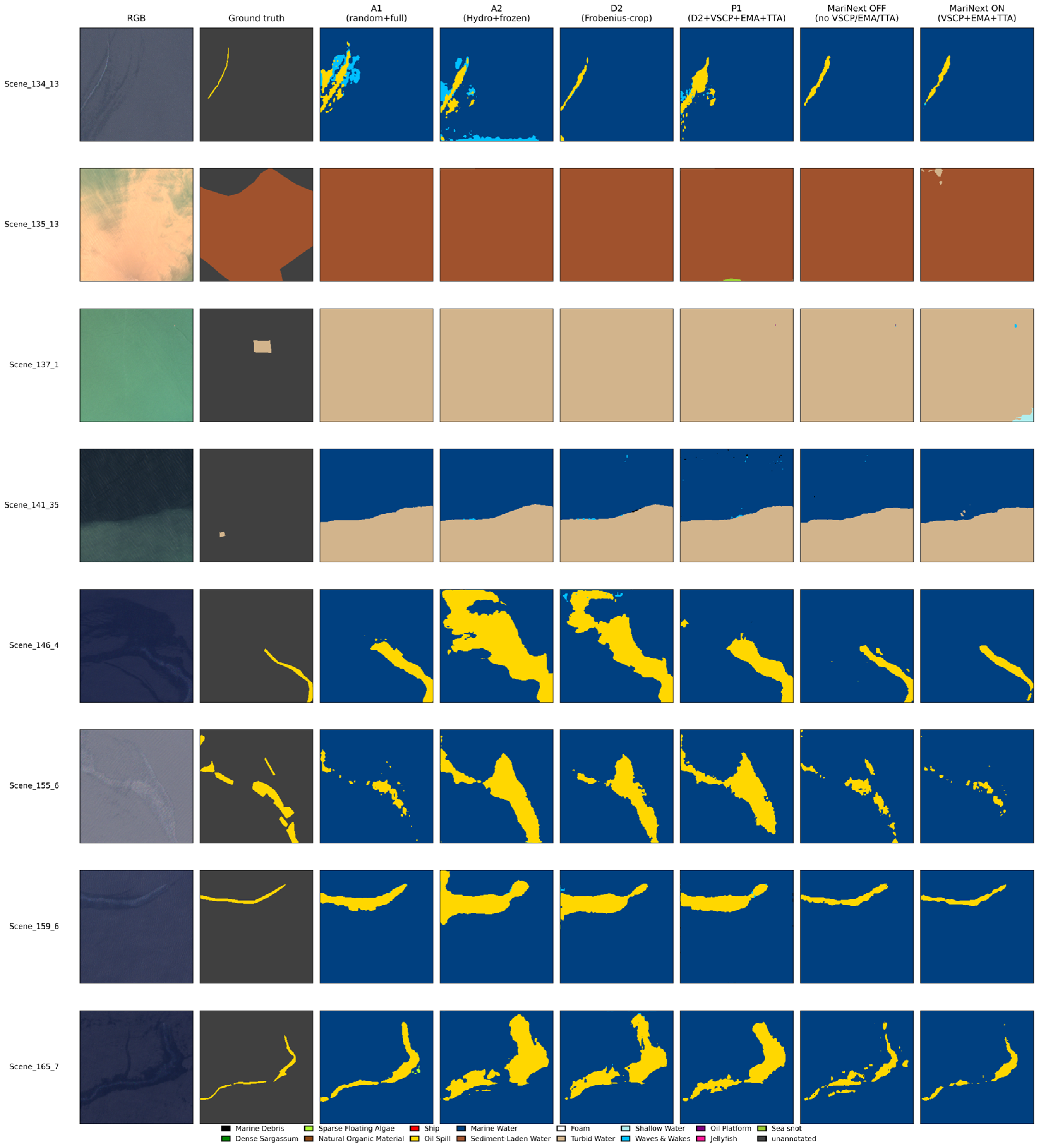
The confusion matrix analysis in Appendix B sharpens this comparison. The published MariNeXt confusion matrix [20] reports 28.3% of oil spill test pixels misclassified as Marine Water. The D2 configuration in the present study reduces this confusion to 5.30%. The opposite direction confusion (Marine Water as oil spill) is 19.8% under D2, indicating that the residual oil spill–Marine Water confusion in the present setting is asymmetric. The model underpredicts oil spill less frequently than it overpredicts it. This is consistent with the band utilisation shift observed in Section 4.4.2, in which Hydro normalisation routes more decision weight to the NIR and SWIR bands where oil–water contrast is largest. Qualitative segmentation outputs for eight representative test patches across the two latent radiometric settings of Section 4.5 are provided in Appendix G, and they visually corroborate the confusion pattern differences quantified above.

5.7. Limitations

Several limitations of the present study should be acknowledged. First, all configurations are trained with two random seeds, and standard deviations computed from two runs carry limited statistical power. The conclusions reported here rest on margins between 0.046 and 0.458 mIoU against cross-seed standard deviations between 0.004 and 0.038; comparisons with smaller margins are reported as indistinguishable throughout. The scene-level bootstrap in Appendix H indicates that the bootstrap standard error exceeds the cross-seed standard deviation in eleven of the twelve configurations examined and is within three per cent of it in the twelfth, so the precision of the reported estimates is limited principally by the number of independent test scenes rather than by seed count. The two comparisons closest to the resolution limit illustrate this directly: paired bootstraps place B1–B2 at +0.011 (95% interval [−0.019, +0.081]) and D2–D3 at +0.019 (95% interval [−0.012, +0.052]), with the sign preserved in 82% and 89% of resamples, respectively. Both orderings are directionally consistent and neither is resolvable against scene-level noise. Replication with additional seeds and evaluation on a larger independent test partition would strengthen the individual comparisons.

Second, while the normalisation mismatch directions have been reported (Section 4.3.2 and Section 5.4), the asymmetry between them is not yet mechanistically resolved. The forward direction loses 80.2% of its clean mIoU against 57.0% in the reverse, and the compression account offered in Section 5.4 is consistent with that ordering without isolating it experimentally. Separating the effect of scale contraction from that of mean offset would require a sweep over the ratio between train-time and test-time normalisation constants, which is left for future work. Third, the MADOS splits were verified to be disjointed at the scene level for the present study; the 174 scenes partition into 96 training, 36 validation, and 42 test scenes, with no scene appearing in more than one split, so the results are not affected by cross-split scene leakage. The test partition is nonetheless small in terms of independent units. Its 42 scenes contribute between two and 48 patches each (median 14.5), and no single scene contains more than eight of the fifteen classes. This is the principal reason the intervals in Appendix H are wide, and it bounds the precision attainable on this benchmark irrespective of training protocol.

Fourth, the spectral importance attribution in Section 4.4.2 uses a zero occlusion (equivalent to MADOS-mean replacement) as the baseline. Alternative baselines such as noise injection may yield different importance rankings. The conclusions drawn here pertain to relative shifts in band utilisation between normalisation strategies, which are less sensitive to the choice of baseline than absolute importance values.

Fifth, the experiments use only the Hydro foundation model and the MADOS dataset. Generalisation of these findings to other foundation models (e.g., Prithvi, SatMAE, SpectralGPT) and multispectral benchmark datasets is not established and is a natural direction for follow-up work.

6. Conclusions

This study examined preprocessing mismatch as a controlled experimental factor in transferring a multispectral foundation model to a marine surface segmentation task. Using the Hydro Swin Transformer V2 encoder and the MADOS benchmark dataset, three preprocessing dimensions (input normalisation, band adaptation, and encoder transfer mode) were systematically varied while all other settings were held constant.

The two datasets are produced by different atmospheric correction algorithms under different reflectance conventions, and the per-band statistical discrepancy that follows is documented in Section 3.1. The controlled experiments were conducted within that setting. Four findings emerge from them. First, the normalisation mismatch between training and inference is the single largest source of performance degradation observed, exceeding all other radiometric perturbations by an order of magnitude. Second, a zero-parameter Frobenius-matched weight crop adapts the 12-band pretrained patch embedding to the 11-band target dataset more effectively than any learnt adapter tested. Third, under limited target data, freezing the encoder outperforms both the fine-tuning in full of the pretrained encoder and the full training from a random initialisation. The gains observed under partially unfrozen configurations are attributable to the augmented training configuration (VSCP, EMA, TTA) rather than to encoder adaptation itself. Fourth, with matched preprocessing, the frozen pretrained encoder matches the published MariNeXt baseline on MADOS within seed variability, demonstrating that careful preprocessing alignment carries most of the practical adaptation effort.

Mechanistic analysis shows that input normalisation alters which spectral bands the encoder relies on, with the magnitude of the shift correlated with the per-band gap between the source and target distributions. This indicates that preprocessing mismatch is not a generic accuracy loss but a structured reweighting of the encoder’s spectral utilisation pattern.

These findings are established for a single encoder–benchmark pair under limited target supervision, and the magnitudes reported should not be read as general constants. The mechanism they identify is the more portable result, whereby a frozen encoder’s representations remain bound to the normalisation statistics of the dataset on which it was pretrained, so any transfer that departs from those statistics at inference should be expected to degrade sharply, and the degradation should scale with the per-band distance between the two distributions. This is testable on any pretrained multispectral encoder with a documented normalisation convention, and it is offered as the generalisable claim of the present work.

Three directions for future work follow. First, the scope of the present study should be extended to additional foundation models and additional multispectral benchmark datasets, in order to establish whether the dominance of normalisation observed here generalises beyond the Hydro–MADOS pair. Second, label-aware harmonisation strategies that explicitly use a small set of target labels to align source and target statistics, rather than the label-free transforms tested on block H, may close more of the mismatch gap. Third, the operational implications of patch-level normalisation fragility (the ability to flag at-risk patches from input statistics alone) warrant integration into deployed marine pollution monitoring pipelines. Fourth, the contribution of atmospheric correction specifically, as distinct from the other differences between the two datasets, could be isolated by processing a common set of scenes through several correction algorithms and repeating the controlled protocol on each.

References

1. Cong, Y.; Khanna, S.; Meng, C.; Liu, P.; Rozi, E.; He, Y.; Burke, M.; Lobell, D.B.; Ermon, S. SatMAE: Pre-Training Transformers for Temporal and Multi-Spectral Satellite Imagery. In Proceedings of the Advances in Neural Information Processing Systems (NeurIPS 2022), New Orleans, LA, USA, 28 November–9 December 2022. [Google Scholar]
2. Jakubik, J.; Roy, S.; Phillips, C.E.; Fraccaro, P.; Godwin, D.; Zadrozny, B.; Szwarcman, D.; Gomes, C.; Nyirjesy, G.; Edwards, B.; et al. Foundation Models for Generalist Geospatial Artificial Intelligence. arXiv 2023, arXiv:2310.18660. [Google Scholar] [CrossRef] [Scilit]
3. Szwarcman, D.; Roy, S.; Fraccaro, P.; Gislason, T.E.; Blumenstiel, B.; Ghosal, R.; de Oliveira, P.H.; de Sousa Almeida, J.L.; Sedona, R.; Kang, Y.; et al. Prithvi-EO-2.0: A Versatile Multitemporal Foundation Model for Earth Observation Applications. IEEE Trans. Geosci. Remote Sens. 2026, 64, 4400120. [Google Scholar] [CrossRef] [Scilit]
4. Guo, X.; Lao, J.; Dang, B.; Zhang, Y.; Yu, L.; Ru, L.; Zhong, L.; Huang, Z.; Wu, K.; Hu, D.; et al. SkySense: A Multi-Modal Remote Sensing Foundation Model Towards Universal Interpretation for Earth Observation Imagery. In Proceedings of the IEEE/CVF Conference on Computer Vision and Pattern Recognition (CVPR), Seattle, WA, USA, 17–21 June 2024; pp. 27672–27683. [Google Scholar]
5. Clay Foundation. Clay Foundation Model: An Open Source AI Foundation Model for Earth. Available online: https://github.com/Clay-foundation/model (accessed on 1 June 2026).
6. Hong, D.; Zhang, B.; Li, X.; Li, Y.; Li, C.; Yao, J.; Yokoya, N.; Li, H.; Ghamisi, P.; Jia, X.; et al. SpectralGPT: Spectral Remote Sensing Foundation Model. IEEE Trans. Pattern Anal. Mach. Intell. 2024, 46, 5227–5244. [Google Scholar] [CrossRef] [Scilit] [PubMed]
7. Corley, I.; Robinson, C. Hydro Foundation Model. 2024. Available online: https://github.com/isaaccorley/hydro-foundation-model (accessed on 1 June 2026).
8. Huo, C.; Chen, K.; Zhang, S.; Wang, Z.; Yan, H.; Shen, J.; Hong, Y.; Qi, G.; Fang, H.; Wang, Z. When Remote Sensing Meets Foundation Model: A Survey and Beyond. Remote Sens. 2025, 17, 179. [Google Scholar] [CrossRef] [Scilit]
9. Zhou, G.; Qian, L.; Gamba, P. Advances on Multimodal Remote Sensing Foundation Models for Earth Observation Downstream Tasks: A Survey. Remote Sens. 2025, 17, 3532. [Google Scholar] [CrossRef] [Scilit]
10. Wang, Y.; Braham, N.A.A.; Xiong, Z.; Liu, C.; Albrecht, C.M.; Zhu, X.X. SSL4EO-S12: A Large-Scale Multi-Modal, Multi-Temporal Dataset for Self-Supervised Learning in Earth Observation. IEEE Geosci. Remote Sens. Mag. 2023, 11, 98–106. [Google Scholar] [CrossRef] [Scilit]
11. Vanhellemont, Q.; Ruddick, K. Atmospheric Correction of Metre-Scale Optical Satellite Data for Inland and Coastal Water Applications. Remote Sens. Environ. 2018, 216, 586–597. [Google Scholar] [CrossRef] [Scilit]
12. Main-Knorn, M.; Pflug, B.; Louis, J.; Debaecker, V.; Müller-Wilm, U.; Gascon, F. Sen2Cor for Sentinel-2. In Proceedings of the SPIE Image and Signal Processing for Remote Sensing XXIII, Warsaw, Poland, 4 October 2017; Volume 10427, p. 1042704. [Google Scholar] [CrossRef] [Scilit]
13. Vermote, E.; Justice, C.; Claverie, M.; Franch, B. Preliminary Analysis of the Performance of the Landsat 8/OLI Land Surface Reflectance Product. Remote Sens. Environ. 2016, 185, 46–56. [Google Scholar] [CrossRef] [Scilit] [PubMed]
14. Hsu, C.-Y.; Li, W.; Wang, S. Geospatial Foundation Models for Image Analysis: Evaluating and Enhancing NASA-IBM Prithvi’s Domain Adaptability. Int. J. Geogr. Inf. Sci. 2025, 39, 2096–2125. [Google Scholar] [CrossRef] [Scilit]
15. Marti-Escofet, F.; Blumenstiel, B.; Scheibenreif, L.; Fraccaro, P.; Schindler, K. Fine-Tune Smarter, Not Harder: Parameter-Efficient Fine-Tuning for Geospatial Foundation Models. In Machine Learning and Knowledge Discovery in Databases; Ribeiro, R.P., Ed.; Research Track. ECML PKDD 2025; Lecture Notes in Computer Science; Springer: Cham, Switzerland, 2025; Volume 16018, pp. 359–375. [Google Scholar] [CrossRef] [Scilit]
16. Al-Ruzouq, R.; Gibril, M.B.A.; Shanableh, A.; Kais, A.; Hamed, O.; Al-Mansoori, S.; Khalil, M.A. Sensors, Features, and Machine Learning for Oil Spill Detection and Monitoring: A Review. Remote Sens. 2020, 12, 3338. [Google Scholar] [CrossRef] [Scilit]
17. Fingas, M.; Brown, C.E. A Review of Oil Spill Remote Sensing. Sensors 2018, 18, 91. [Google Scholar] [CrossRef] [Scilit] [PubMed]
18. Garcia-Pineda, O.; Staples, G.; Jones, C.E.; Hu, C.; Holt, B.; Kourafalou, V.; Graettinger, G.; DiPinto, L.; Ramirez, E.; Streett, D.; et al. Classification of Oil Spill by Thicknesses Using Multiple Remote Sensors. Remote Sens. Environ. 2020, 236, 111421. [Google Scholar] [CrossRef] [Scilit]
19. Sun, S.; Hu, C.; Garcia-Pineda, O.; Kourafalou, V.; Le Hénaff, M.; Androulidakis, Y. Remote Sensing Assessment of Oil Spills near a Damaged Platform in the Gulf of Mexico. Mar. Pollut. Bull. 2018, 136, 141–151. [Google Scholar] [CrossRef] [Scilit] [PubMed]
20. Kikaki, K.; Kakogeorgiou, I.; Hoteit, I.; Karantzalos, K. Detecting Marine Pollutants and Sea Surface Features with Deep Learning in Sentinel-2 Imagery. ISPRS J. Photogramm. Remote Sens. 2024, 210, 39–54. [Google Scholar] [CrossRef] [Scilit]
21. Liu, Z.; Hu, H.; Lin, Y.; Yao, Z.; Xie, Z.; Wei, Y.; Ning, J.; Cao, Y.; Zhang, Z.; Dong, L.; et al. Swin Transformer V2: Scaling Up Capacity and Resolution. In Proceedings of the IEEE/CVF Conference on Computer Vision and Pattern Recognition (CVPR), New Orleans, LA, USA, 18–24 June 2022; pp. 12009–12019. [Google Scholar] [CrossRef] [Scilit]
22. Xie, Z.; Zhang, Z.; Cao, Y.; Lin, Y.; Bao, J.; Yao, Z.; Dai, Q.; Hu, H. SimMIM: A Simple Framework for Masked Image Modeling. In Proceedings of the IEEE/CVF Conference on Computer Vision and Pattern Recognition (CVPR), New Orleans, LA, USA, 18–24 June 2022; pp. 9643–9653. [Google Scholar] [CrossRef] [Scilit]
23. Kolokoussis, P.; Karathanassi, V. Oil Spill Detection and Mapping Using Sentinel 2 Imagery. J. Mar. Sci. Eng. 2018, 6, 4. [Google Scholar] [CrossRef] [Scilit]
24. Rajendran, S.; Sadooni, F.N.; Al-Kuwari, H.-A.-S.; Oleg, A.; Govil, H.; Nasir, S.; Vethamony, P. Monitoring Oil Spill in Norilsk, Russia Using Satellite Data. Sci. Rep. 2021, 11, 3817. [Google Scholar] [CrossRef] [Scilit] [PubMed]
25. Kikaki, K.; Kakogeorgiou, I.; Mikeli, P.; Raitsos, D.E.; Karantzalos, K. MARIDA: A Benchmark for Marine Debris Detection from Sentinel-2 Remote Sensing Data. PLoS ONE 2022, 17, e0262247. [Google Scholar] [CrossRef] [Scilit] [PubMed]
26. Hu, E.J.; Shen, Y.; Wallis, P.; Allen-Zhu, Z.; Li, Y.; Wang, S.; Wang, L.; Chen, W. LoRA: Low-Rank Adaptation of Large Language Models. In Proceedings of the International Conference on Learning Representations (ICLR), Virtual, 25–29 April 2022. [Google Scholar]
27. Jia, M.; Tang, L.; Chen, B.-C.; Cardie, C.; Belongie, S.; Hariharan, B.; Lim, S.-N. Visual Prompt Tuning. In Computer Vision—ECCV 2022; Avidan, S., Brostow, G., Cissé, M., Farinella, G.M., Hassner, T., Eds.; Lecture Notes in Computer Science; Springer: Cham, Switzerland, 2022; Volume 13693, pp. 709–727. [Google Scholar] [CrossRef] [Scilit]
28. Houlsby, N.; Giurgiu, A.; Jastrzebski, S.; Morrone, B.; De Laroussilhe, Q.; Gesmundo, A.; Attariyan, M.; Gelly, S. Parameter-Efficient Transfer Learning for NLP. In Proceedings of the International Conference on Machine Learning (ICML), Long Beach, CA, USA, 9–15 June 2019; pp. 2790–2799. [Google Scholar]
29. Thoreau, R.; Marsocci, V.; Derksen, D. Parameter-Efficient Adaptation of Geospatial Foundation Models through Embedding Deflection. In Proceedings of the IEEE/CVF International Conference on Computer Vision (ICCV), Honolulu, HI, USA, 19–25 October 2025. [Google Scholar] [CrossRef] [Scilit]
30. Sun, B.; Saenko, K. Deep CORAL: Correlation Alignment for Deep Domain Adaptation. In Computer Vision—ECCV 2016 Workshops; Hua, G., Jégou, H., Eds.; Lecture Notes in Computer Science; Springer: Cham, Switzerland, 2016; Volume 9915, pp. 443–450. [Google Scholar] [CrossRef] [Scilit]
31. Li, Y.; Wang, N.; Shi, J.; Liu, J.; Hou, X. Revisiting Batch Normalization for Practical Domain Adaptation. In Proceedings of the International Conference on Learning Representations (ICLR) Workshop, Toulon, France, 24–26 April 2017. [Google Scholar]
32. Tuia, D.; Persello, C.; Bruzzone, L. Domain Adaptation for the Classification of Remote Sensing Data: An Overview of Recent Advances. IEEE Geosci. Remote Sens. Mag. 2016, 4, 41–57. [Google Scholar] [CrossRef] [Scilit]
33. Geng, Z.; Guo, M.-H.; Chen, H.; Li, X.; Wei, K.; Lin, Z. Is Attention Better Than Matrix Decomposition? In Proceedings of the International Conference on Learning Representations (ICLR), Virtual, 25–29 April 2022. [Google Scholar]
34. Breiman, L. Random Forests. Mach. Learn. 2001, 45, 5–32. [Google Scholar] [CrossRef] [Scilit]
35. Zeiler, M.D.; Fergus, R. Visualizing and Understanding Convolutional Networks. In Computer Vision—ECCV 2014; Fleet, D., Pajdla, T., Schiele, B., Tuytelaars, T., Eds.; Lecture Notes in Computer Science; Springer: Cham, Switzerland, 2014; Volume 8689, pp. 818–833. [Google Scholar] [CrossRef] [Scilit]
36. Asadzadeh, S.; de Souza Filho, C.R. Investigating the Capability of WorldView-3 Superspectral Data for Direct Hydrocarbon Detection. Remote Sens. Environ. 2016, 173, 162–173. [Google Scholar] [CrossRef] [Scilit]
Figure 1. Architecture diagram.
Remotesensing 18 02905 g001
Figure 2. UMAP projection of pre-HAM decoder features (seed 0). Three panels: B1 (MADOS normalisation, no adapter), B2 (Hydro normalisation, no adapter), and D2 (MADOS normalisation, Frobenius-matched crop). Four classes are highlighted: oil spill (red), Marine Water (blue), Shallow Water (purple), Waves and Wakes (green). Axes are UMAP dimension components 1 and 2 in arbitrary units.
Remotesensing 18 02905 g002
Figure 3. Per-band-occlusion importance for oil spill, seed 0, in three settings: top, frozen Hydro encoder without adapter (B1 versus B2); middle, frozen Hydro encoder with D3 linear adapter (E2 versus G2 mirror); bottom, evaluation under both normalisation strategies. Blue bars: MADOS normalisation. Red bars: Hydro normalisation. The NIR-SWIR region is shaded.
Remotesensing 18 02905 g003