


GeoAI-Driven Wetland Change Analysis in the Sangamon River Watershed (2000–2025): A Comparative Assessment of Machine Learning and Deep Learning Approaches


Highlights
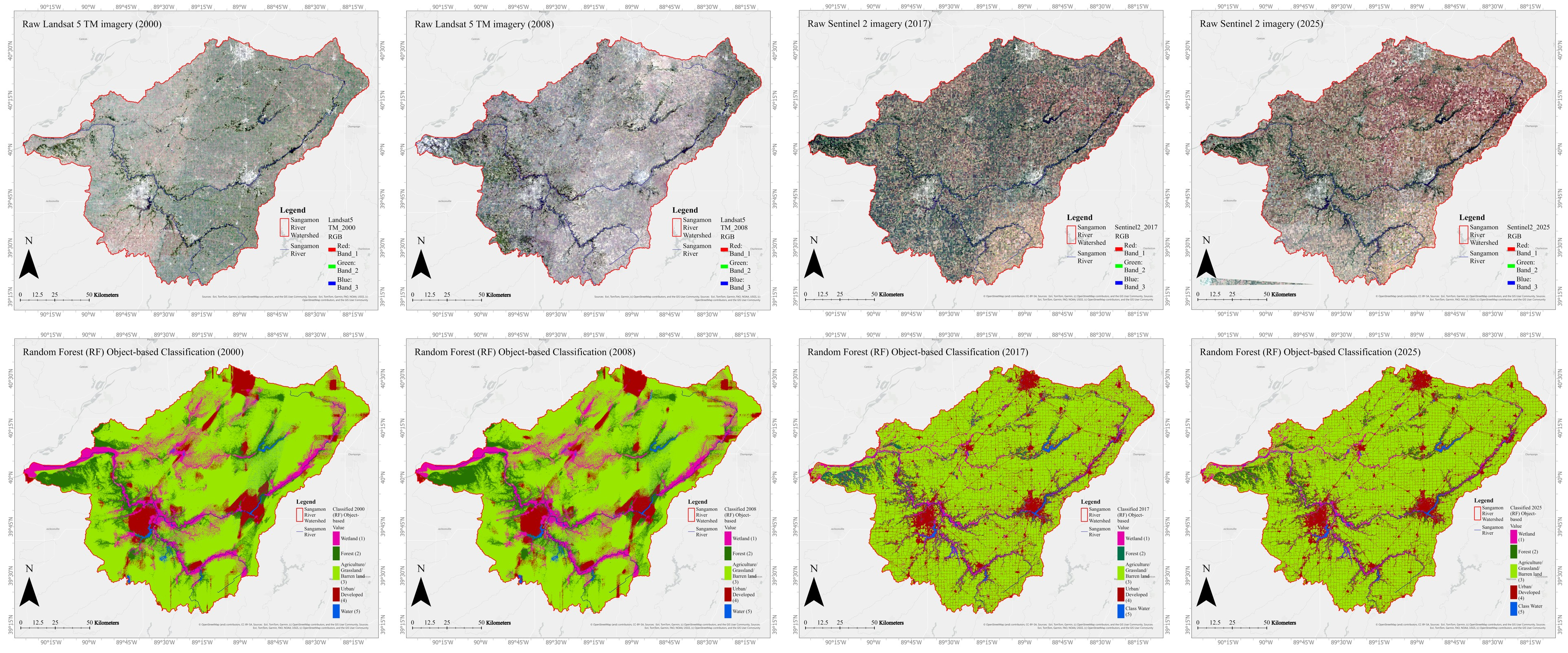
- The Sangamon River Watershed experienced major landscape transformation over 25 years, including a loss of 54.85% of wetland extent (860.68 km2), 46.51% of forest cover (694.88 km2), and 36.8% of water bodies (66.13 km2), alongside substantial increases in agriculture/grassland/barren land 8.56% (820.62 km2) and urban/developed areas 72.92% (799.52 km2).
- A comparative GeoAI framework integrating multi–source Earth observations, object–based image analysis, ML, CNNs, and transformer–based DL models demonstrated that transformer-based models achieved superior segmentation of spatially fragmented and spectrally heterogeneous wetlands and land–cover classes.
- The findings show the potential of advanced GeoAI and multi–source Earth observation for accurate, scalable, and transferable watershed–scale wetland monitoring and landuse change analysis.
- Results provide valuable geospatial insights for wetland conservation, restoration, and climate–resilient watershed planning in agriculturally dominated watersheds.
Abstract
1. Introduction
- Integrating multi-season Landsat 5 TM (for years 2000–2008) and Sentinel-2 (for years 2017–2025) optical indices, Sentinel-1 SAR backscatter, GLCM, and terrain-derived variables within a comparative ML through both pixel-based and object-based approaches and core and advanced DL-based workflows to evaluate their accuracy performance in wetland mapping and change detection.
- Investigating the contribution of Sentinel-1 SAR data when integrated with Sentinel-2, terrain, and GLCM variables to determine its effectiveness for wetland classification in agriculture-dominated landscapes.
- ▪ Applying a temporally consistent classification approach using identical predictors, training data for 2001 and 2017, and classification methodology to ensure that changes reflect true land cover transitions.
- Evaluating DL models performance against ML models for Landsat 5 TM and Sentinel-2, respectively, for different spatial resolutions, and temporal periods, sensor characteristics, and model architectures.
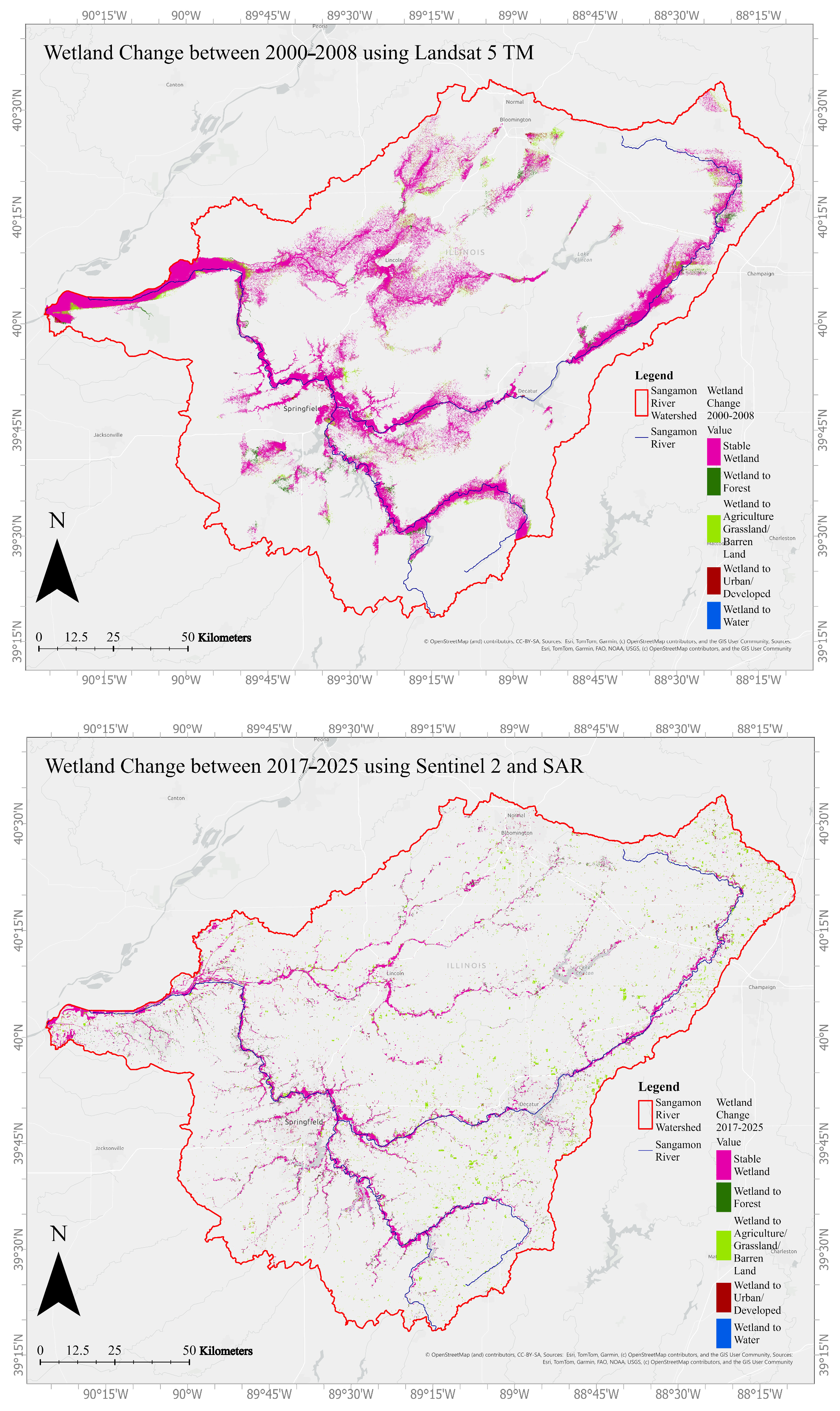
- Quantifies and spatially characterizes wetland dynamics, including gains, losses, and conversions to other land use types, providing critical understanding into landscape-level transformations.
- Integrating cloud-based GEE and Colab platforms that provide high computational efficiency with ArcGIS-based visualization and quantification.
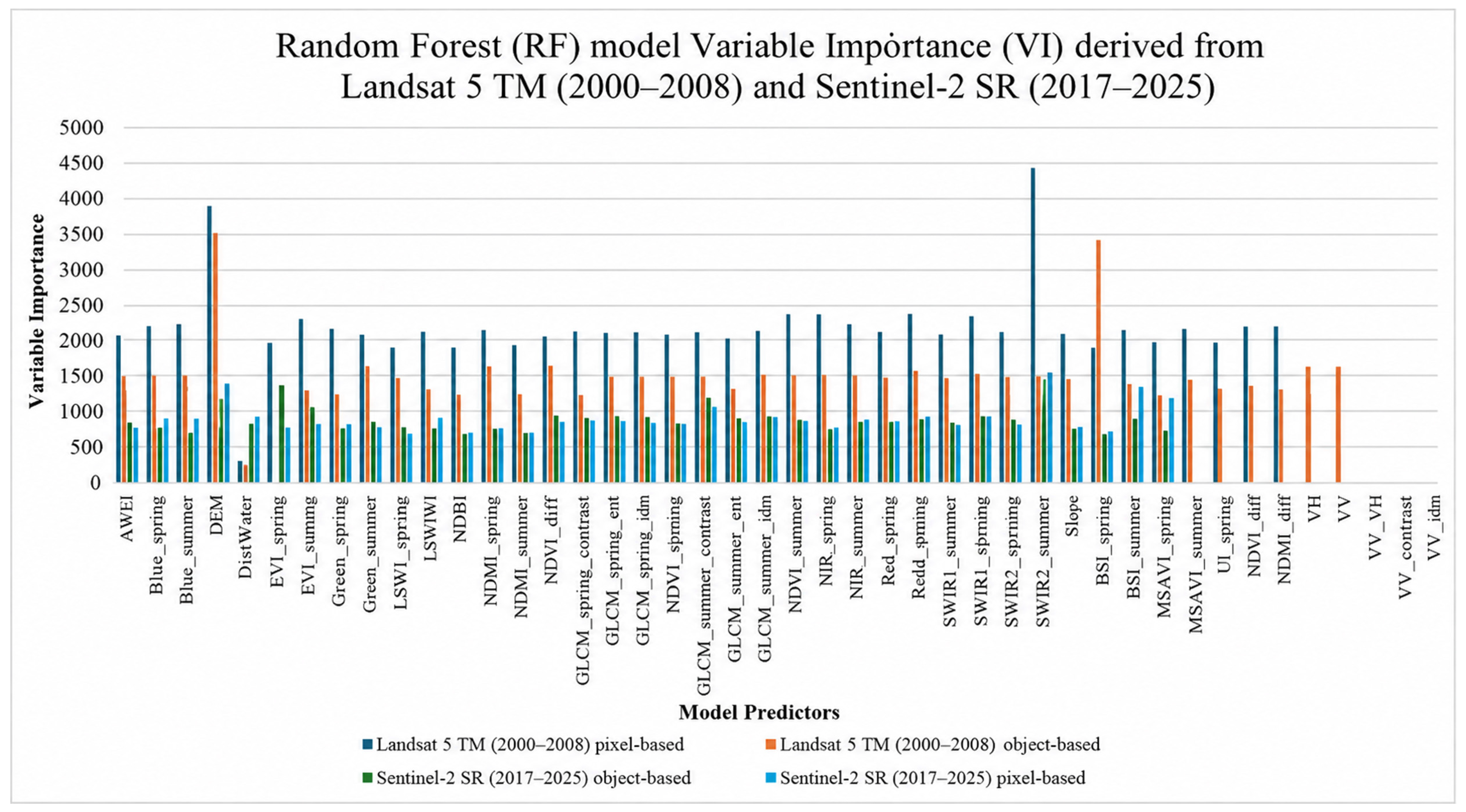
- ▪ Determining the “variable importance” of variables used in this study through the RF classifier algorithm.
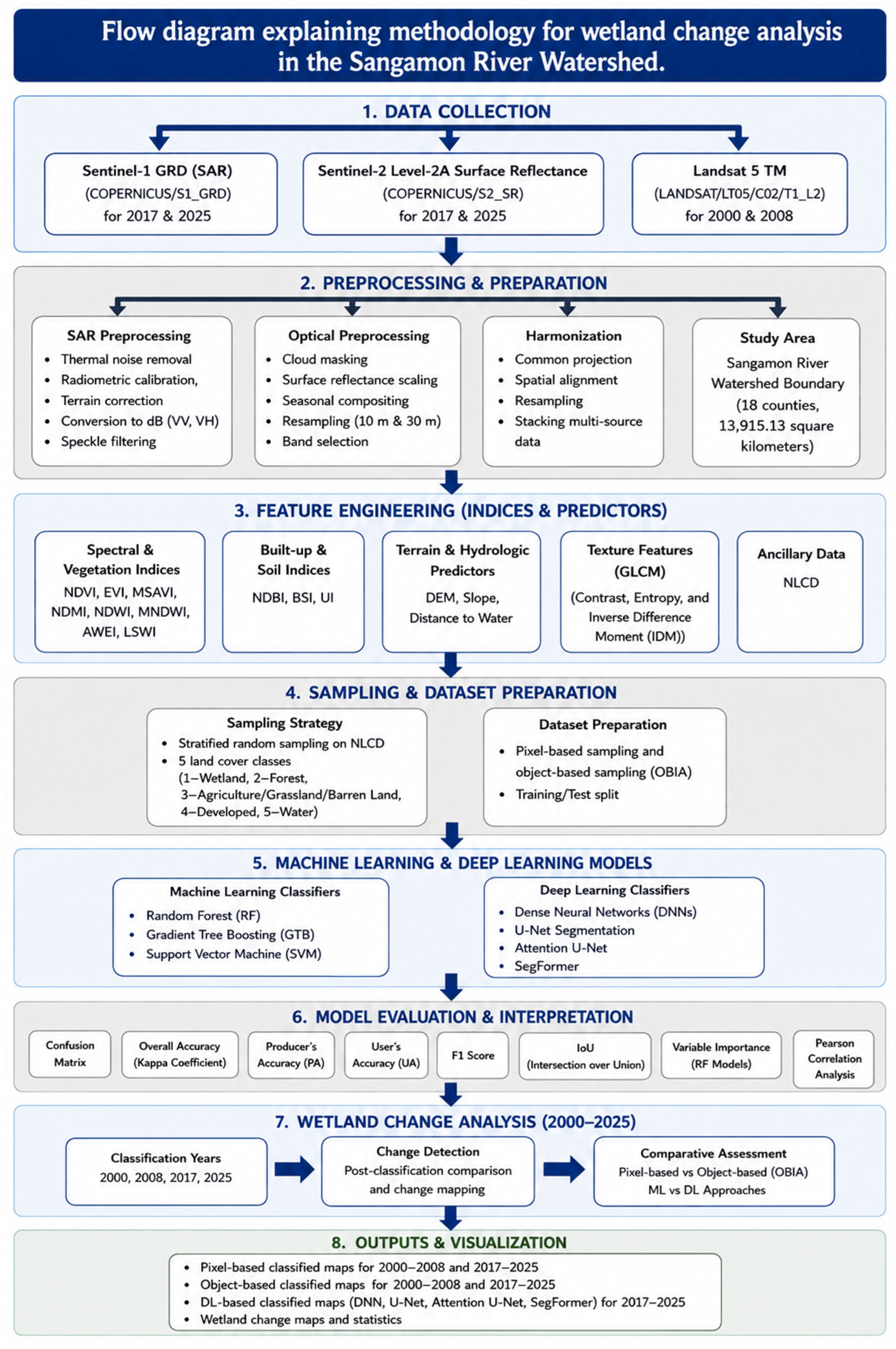
2. Methods
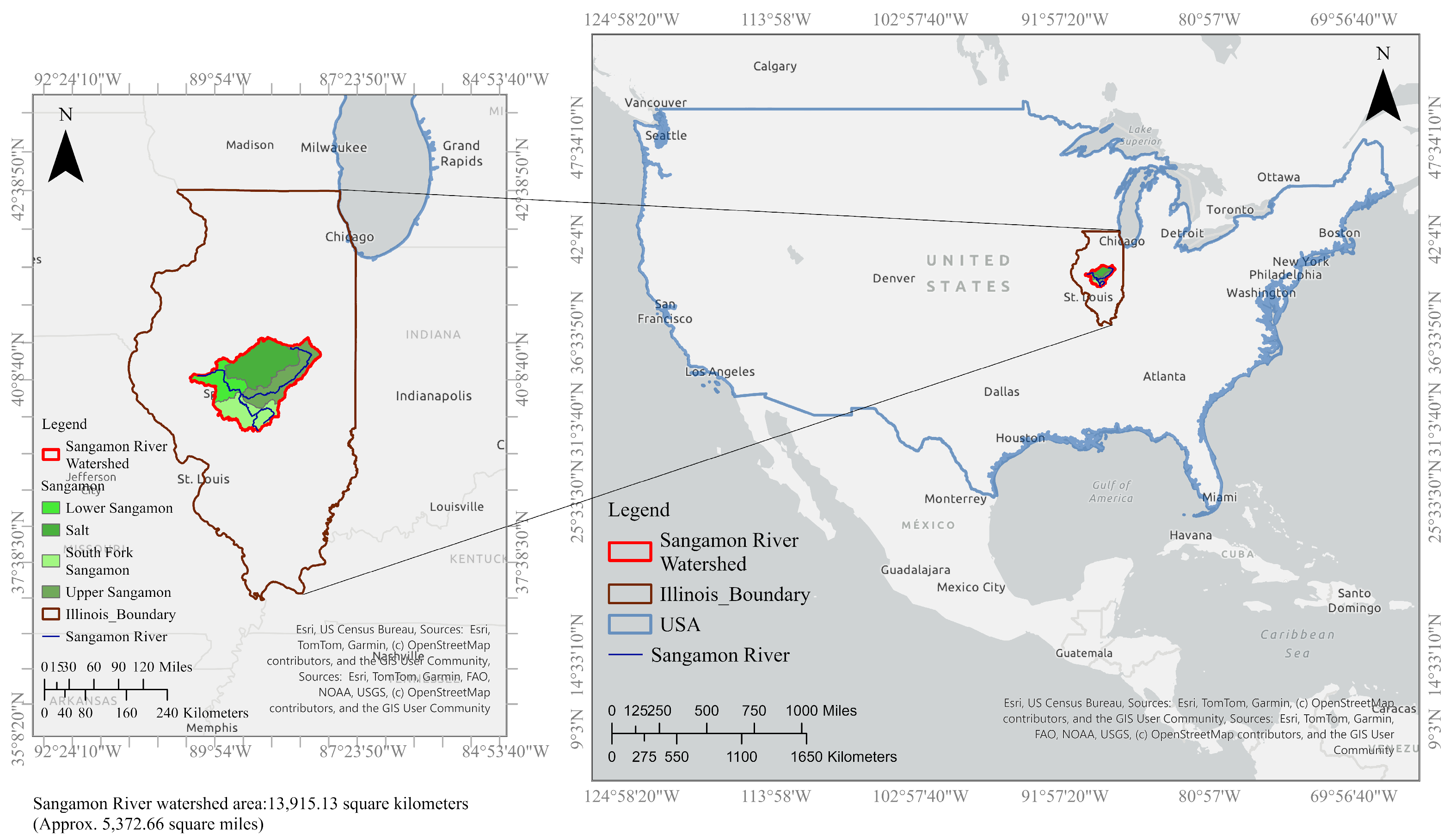
2.1. Study Area (Sangamon River Watershed)
2.2. Data Sources and Data Processing
2.3. Cloud Masking, Surface Reflectance Scaling and Band Selection
2.4. Composite Generation and Normalization
2.5. DNN, Attention U-Net and SegFormer Semantic Segmentation for Landsat 5 TM (2000–2008)
2.6. U-Net, Attention U-Net, and SegFormer Semantic Segmentation for Sentinel–2 and Sentinel–1 Data (2017–2025)
2.7. Spectral Indices
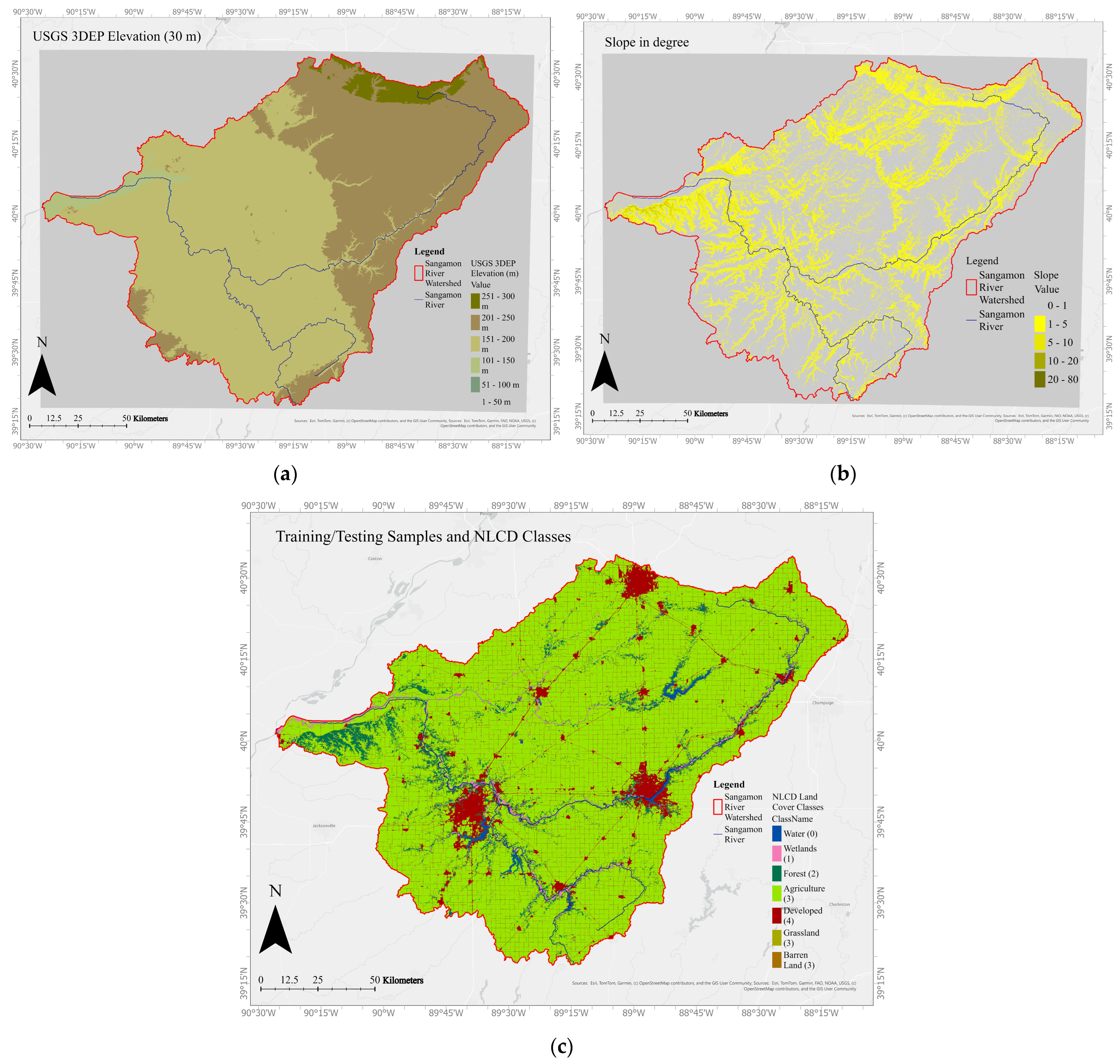
2.8. Digital Elevation Model (DEM), Slope, and Distance–to–Water
2.9. Gray-Level Co-Occurrence Matrix (GLCM)
2.10. Training Samples
2.11. Training ML and DL Classifiers for Classifying Maps (2000–2008–2017–2025)
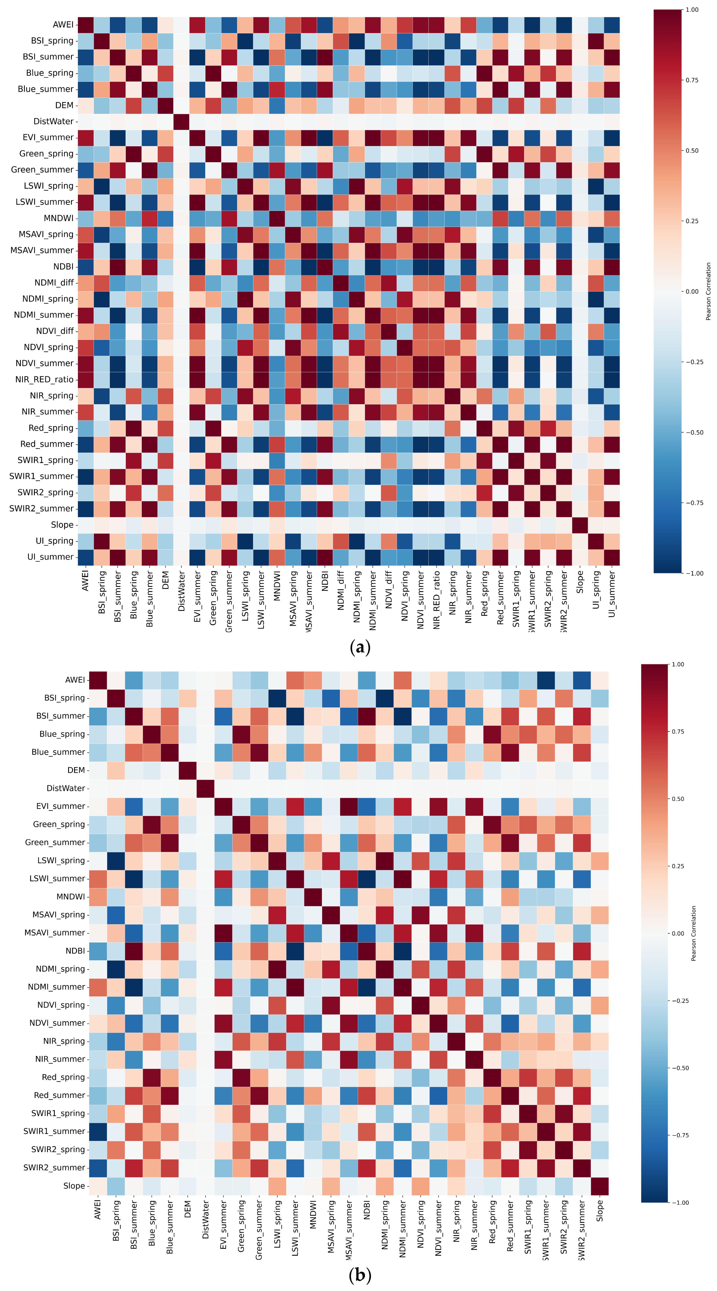
2.12. Pearsons Correlation Analysis
3. Results
3.1. Accuracy Assessment
3.2. Landsat 5 TM for Period 2000–2008
3.3. Sentinel–2 for Period 2017–2025
3.4. Variable Importance (VI) and Relative Importance (RI) in RF Models
3.4.1. Landsat 5 TM (2000–2008)
3.4.2. Sentinel-2 SR (2017–2025)
3.5. Change Detection and Wetland Loss Calculations (2000–2008–2017–2025)
4. Discussion
5. Conclusions
Author Contributions
Funding
Data Availability Statement
Acknowledgments
Conflicts of Interest
Abbreviations
| ANN | Artificial neural network |
| AWEI | Automated Water Extraction Index |
| BSI | Bare Soil Index |
| CART | Classification and regression tree |
| CM | Confusion matrix |
| FCN | Fully convolutional network |
| CNN | Convolutional neural network |
| DL | Deep learning |
| DNN | Dense neural network |
| DEM | Digital elevation model |
| DEP | Digital elevation product |
| EVI | Enhanced Vegetation Index |
| GEE | Google Earth Engine |
| GTB | Gradient tree boosting |
| GLCM | Gray-level co-occurrence matrix |
| GRD | Ground range detected |
| HUC | Hydrologic unit code |
| IDM IMLCZO | Inverse difference moment Intensively Managed Landscapes Critical Zone Observatory |
| KC | Kappa coefficient |
| LSWI | Land Surface Water Index |
| LULC | Land Use and Land Cover |
| L5 LiDAR | Landsat 5 Light Detection and Ranging |
| ML | Machine learning |
| MNDWI | Modified Normalized Difference Water Index |
| MSAVI | Modified Soil Adjusted Vegetation Index |
| NLCD | National Land Cover Database |
| NIR | Near infrared |
| NDBI | Normalized Difference Built-up Index |
| NDMI | Normalized Difference Moisture Index |
| NDVI | Normalized Difference Vegetation Index |
| NAD | North American Datum |
| OBIA | Object-based image analysis |
| OA | Overall accuracy |
| PA | Producer’s accuracy |
| QA | Quality assessment |
| RF | Random forest |
| RNN | Recurrent neural network |
| RI | Relative importance |
| SLR | Sea-level rise |
| S2 | Sentinel-2 |
| SWIR | Short wave infrared |
| SVM | Support vector machine |
| SR | Surface reflectance |
| SAR | Synthetic aperture radar |
| TFRecord | TensorFlow record |
| TM | Thematic mapper |
| US | United States |
| USGS | United States Geological Survey |
| UI | Urban Index |
| UA | User’s accuracy |
| VI | Variable importance |
References
- Groot, R.D.; Stuip, M.; Finlayson, M.; Davidson, N. Valuing Wetlands: Guidance for Valuing the Benefits Derived from Wetland Ecosystem Services; Secretariat of the Convention on Wetlands: Gland, Switzerland; Secretariat of the Convention on Biological Diversity: Montreal, QC, Canada, 2006; pp. 2–45. [Google Scholar]
- Mitsch, W.J.; Bernal, B.; Hernandez, M.E. Ecosystem services of wetlands. Int. J. Biodivers. Sci. Ecosyst. Serv. Manag. 2015, 11, 1–4. [Google Scholar] [CrossRef] [Scilit]
- Barbier, E.B. The value of coastal wetland ecosystem services. In Coastal Wetlands; Elsevier: Amsterdam, The Netherlands, 2019; pp. 947–964. [Google Scholar]
- Xu, X.; Chen, M.; Yang, G.; Jiang, B.; Zhang, J. Wetland ecosystem services research: A critical review. Glob. Ecol. Conserv. 2020, 22, e01027. [Google Scholar] [CrossRef] [Scilit]
- Ballut–Dajud, G.A.; Sandoval Herazo, L.C.; Fernández–Lambert, G.; Marín–Muñiz, J.L.; López Méndez, M.C.; Betanzo–Torres, E.A. Factors affecting wetland loss: A review. Land 2022, 11, 434. [Google Scholar] [CrossRef] [Scilit]
- Dahl, T.E. Wetlands losses in the United States, 1780’s to 1980’s; US Department of the Interior, Fish and Wildlife Service: Washington, DC, USA, 1990.
- Gibbs, J.P. Wetland loss and biodiversity conservation. Conserv. Biol. 2000, 14, 314–317. [Google Scholar] [CrossRef] [Scilit]
- Zedler, J.B.; Kercher, S. Wetland RESOURCES: Status, trends, ecosystem services, and restorability. Annu. Rev. Environ. Resour. 2005, 30, 39–74. [Google Scholar] [CrossRef] [Scilit]
- Hu, S.; Niu, Z.; Chen, Y.; Li, L.; Zhang, H. Global wetlands: Potential distribution, wetland loss, and status. Sci. Total Environ. 2017, 586, 319–327. [Google Scholar] [CrossRef] [Scilit]
- Fluet–Chouinard, E.; Stocker, B.D.; Zhang, Z.; Malhotra, A.; Melton, J.R.; Poulter, B.; Kaplan, J.O.; Goldewijk, K.K.; Siebert, S.; Minayeva, T.; et al. Extensive global wetland loss over the past three centuries. Nature 2023, 614, 281–286. [Google Scholar] [CrossRef] [Scilit]
- Wilkening, J.L.; Esralew, R.A.; Newman, B.F. From assessment to action: Informing water resource management in protected areas amid global change. Front. Water 2026, 7, 1719814. [Google Scholar] [CrossRef] [Scilit]
- Groschen, G.E.; Harris, M.A.; King, R.B.; Terrio, P.J.; Warner, K.L. Water Quality in the Lower Illinois River Basin, Illinois, 1995–1998; (No. 1209); US Geological Survey: Reston, VA, USA, 2000.
- Borah, D.K.; Bera, M.; Shaw, S. Water, sediment, nutrient, and pesticide measurements in an agricultural watershed in Illinois during storm events. Trans. ASAE 2003, 46, 657. [Google Scholar] [CrossRef] [Scilit]
- Dahl, T.E.; Allord, G.J. History of wetlands in the conterminous United States. In National Water Summary on Wetland Resources Water–Supply Paper 2425; Fretwell, J.D., Williams, J.S., Redman, P.J., Eds.; U.S. Geological Survey: Washington, DC, USA, 1996; pp. 19–25. [Google Scholar]
- Farda, N.M. Multi–temporal land use mapping of coastal wetlands area using machine learning in Google earth engine. In IOP Conference Series: Earth and Environmental Science; IOP Publishing: Bristol, UK, 2017; Volume 98, p. 012042. [Google Scholar]
- Salas, E.A.L.; Kumaran, S.S.; Bennett, R.; Willis, L.P.; Mitchell, K. Machine learning–based classification of small–sized wetlands using Sentinel–2 images. AIMS Geosci. 2024, 10, 62. [Google Scholar] [CrossRef] [Scilit]
- Mahdianpari, M.; Granger, J.E.; Mohammadimanesh, F.; Salehi, B.; Brisco, B.; Homayouni, S.; Gill, E.; Huberty, B.; Lang, M. Meta–Analysis of wetland classification using remote sensing: A systematic review of a 40–Year trend in North America. Remote Sens. 2020, 12, 1882. [Google Scholar] [CrossRef] [Scilit]
- Jafarzadeh, H.; Mahdianpari, M.; Gill, E.W.; Brisco, B.; Mohammadimanesh, F. Remote sensing and machine learning tools to support wetland monitoring: A meta–analysis of three decades of research. Remote Sens. 2022, 14, 6104. [Google Scholar] [CrossRef] [Scilit]
- Day, J.W.; Britsch, L.D.; Hawes, S.R.; Shaffer, G.P.; Reed, D.J.; Cahoon, D. Pattern and process of land loss in the Mississippi Delta: A spatial and temporal analysis of wetland habitat change. Estuaries 2000, 23, 425–438. [Google Scholar] [CrossRef] [Scilit]
- Montgomery, J.; Mahoney, C.; Brisco, B.; Boychuk, L.; Cobbaert, D.; Hopkinson, C. Remote sensing of wetlands in the prairie pothole region of North America. Remote Sens. 2021, 13, 3878. [Google Scholar] [CrossRef] [Scilit]
- Ballanti, L.; Byrd, K.B.; Woo, I.; Ellings, C. Remote sensing for wetland mapping and historical change detection at the Nisqually River Delta. Sustainability 2017, 9, 1919. [Google Scholar] [CrossRef] [Scilit]
- Mattson, M.; Sousa, D.; Quandt, A.; Ganster, P.; Biggs, T. Mapping multi–decadal wetland loss: Comparative analysis of linear and nonlinear spatiotemporal characterization. Remote Sens. Environ. 2024, 302, 113969. [Google Scholar] [CrossRef] [Scilit]
- Ghorbanian, A.; Zaghian, S.; Asiyabi, R.M.; Amani, M.; Mohammadzadeh, A.; Jamali, S. Mangrove ecosystem mapping using Sentinel–1 and Sentinel–2 satellite images and random forest algorithm in Google Earth Engine. Remote Sens. 2021, 13, 2565. [Google Scholar] [CrossRef] [Scilit]
- Mahdianpari, M.; Jafarzadeh, H.; Granger, J.E.; Mohammadimanesh, F.; Brisco, B.; Salehi, B.; Homayouni, S.; Weng, Q. A large–scale change monitoring of wetlands using time series Landsat imagery on Google Earth Engine: A case study in Newfoundland. GISci. Remote Sens. 2020, 57, 1102–1124. [Google Scholar] [CrossRef] [Scilit]
- Chasmer, L.; Mahoney, C.; Millard, K.; Nelson, K.; Peters, D.; Merchant, M.; Hopkinson, C.; Brisco, B.; Niemann, O.; Montgomery, J.; et al. Remote sensing of boreal wetlands 2: Methods for evaluating boreal wetland ecosystem State and drivers of change. Remote Sens. 2020, 12, 1321. [Google Scholar] [CrossRef] [Scilit]
- Zerrouk, M.; Ait El Kadi, K.; Sebari, I.; Fellahi, S. Machine and Deep Learning for Wetland Mapping and Bird–Habitat Monitoring: A Systematic Review of Remote–Sensing Applications (2015–April 2025). Remote Sens. 2025, 17, 3605. [Google Scholar] [CrossRef] [Scilit]
- Pashaei, M.; Kamangir, H.; Starek, M.J.; Tissot, P. Review and evaluation of deep learning architectures for efficient land cover mapping with UAS hyper–spatial imagery: A case study over a wetland. Remote Sens. 2020, 12, 959. [Google Scholar] [CrossRef] [Scilit]
- Fickas, K.C.; Cohen, W.B.; Yang, Z. Landsat–based monitoring of annual wetland change in the Willamette Valley of Oregon, USA from 1972 to 2012. Wetl. Ecol. Manag. 2016, 24, 73–92. [Google Scholar] [CrossRef] [Scilit]
- Sultana, S.; Inayathulla, M. Precision land use and land cover classification using Google Earth Engine: Integrating random forest and support vector machine algorithms. Geo. Eye 2022, 11, 9–14. [Google Scholar] [CrossRef] [Scilit]
- Rodriguez–Galiano, V.F.; Ghimire, B.; Rogan, J.; Chica–Olmo, M.; Rigol–Sanchez, J.P. An assessment of the effectiveness of a random forest classifier for land–cover classification. ISPRS J. Photogramm. Remote Sens. 2012, 67, 93–104. [Google Scholar] [CrossRef] [Scilit]
- Delalay, M.; Tiwari, V.; Ziegler, A.D.; Gopal, V.; Passy, P. Land–use and land–cover classification using Sentinel–2 data and machine–learning algorithms: Operational method and its implementation for a mountainous area of Nepal. J. Appl. Remote Sens. 2019, 13, 014530. [Google Scholar] [CrossRef] [Scilit]
- Tu, Y.; Lang, W.; Yu, L.; Li, Y.; Jiang, J.; Qin, Y.; Wu, J.; Chen, T.; Xu, B. Improved mapping results of 10 m resolution land cover classification in Guangdong, China using multisource remote sensing data with Google Earth Engine. IEEE J. Sel. Top. Appl. Earth Obs. Remote Sens. 2020, 13, 5384–5397. [Google Scholar] [CrossRef] [Scilit]
- Talukdar, S.; Singha, P.; Mahato, S.; Pal, S.; Liou, Y.A.; Rahman, A. Land–use land–cover classification by machine learning classifiers for satellite observations–A review. Remote Sens. 2020, 12, 1135. [Google Scholar] [CrossRef] [Scilit]
- Sultan, M.; Saleous, N.; Issa, S.; Dahy, B.; Sami, M. Optimizing land use classification using Google Earth Engine: A comparative analysis of machine learning algorithms. ISPRS Ann. Photogramm. Remote Sens. Spat. Inf. Sci. 2025, X-G-2025, 863–869. [Google Scholar] [CrossRef] [Scilit]
- Yuan, S.; Liang, X.; Lin, T.; Chen, S.; Liu, R.; Wang, J.; Zhang, H.; Gong, P. A comprehensive review of remote sensing in wetland classification and mapping. arXiv 2025, arXiv:2504.10842. [Google Scholar]
- Zelioli, L.; Farahnakian, F.; Middleton, M.; Pitkänen, T.P.; Tuominen, S.; Nevalainen, P.; Pohjankukka, J.; Heikkonen, J. Peatland pixel–level classification via multispectral, multiresolution and multisensor data using convolutional neural network. Ecol. Inform. 2025, 90, 103233. [Google Scholar] [CrossRef] [Scilit]
- Merchant, M.A.; Evans, J.; Edwards, R.; Boychuk, L.; Simms, J.; Hird, J.N.; Dooley, J.; Doan, T.; Toni, S.; Cobbaert, D.; et al. AI–Driven Wetland Mapping Across Diverse Natural Regions of Alberta, Canada, Using Combined Airborne and Satellite Remote Sensing Data. Remote Sens. 2026, 18, 507. [Google Scholar] [CrossRef] [Scilit]
- Wang, B.; Sun, Y.; Zhu, X.; Teng, S.; Li, Y. A modified Swin–UNet model for coastal wetland classification using multi–temporal Sentinel–2 images. Estuaries Coasts 2025, 48, 72. [Google Scholar] [CrossRef] [Scilit]
- Lin, X.; Cheng, Y.; Chen, G.; Chen, W.; Chen, R.; Gao, D.; Zhang, Y.; Wu, Y. Semantic segmentation of China’s coastal wetlands based on Sentinel–2 and Segformer. Remote Sens. 2023, 15, 3714. [Google Scholar] [CrossRef] [Scilit]
- Jamali, A.; Mahdianpari, M.; Brisco, B.; Mao, D.; Salehi, B.; Mohammadimanesh, F. 3DUNetGSFormer: A deep learning pipeline for complex wetland mapping using generative adversarial networks and Swin transformer. Ecol. Inform. 2022, 72, 101904. [Google Scholar] [CrossRef] [Scilit]
- Zhao, Z.; Islam, F.; Waseem, L.A.; Tariq, A.; Nawaz, M.; Islam, I.U.; Bibi, T.; Rehman, N.U.; Ahmad, W.; Aslam, R.W.; et al. Comparison of three machine learning algorithms using google earth engine for land use land cover classification. Rangel. Ecol. Manag. 2024, 92, 129–137. [Google Scholar] [CrossRef] [Scilit]
- Dronova, I. Object–based image analysis in wetland research: A review. Remote Sens. 2015, 7, 6380–6413. [Google Scholar] [CrossRef] [Scilit]
- Hossain, M.D.; Chen, D. Segmentation for Object–Based Image Analysis (OBIA): A review of algorithms and challenges from remote sensing perspective. ISPRS J. Photogramm. Remote Sens. 2019, 150, 115–134. [Google Scholar] [CrossRef] [Scilit]
- Duro, D.C.; Franklin, S.E.; Dubé, M.G. A comparison of pixel–based and object–based image analysis with selected machine learning algorithms for the classification of agricultural landscapes using SPOT–5 HRG imagery. Remote Sens. Environ. 2012, 118, 259–272. [Google Scholar] [CrossRef] [Scilit]
- Zheng, J.-Y.; Hao, Y.-Y.; Wang, Y.-C.; Zhou, S.-Q.; Wu, W.-B.; Yuan, Q.; Gao, Y.; Guo, H.-Q.; Cai, X.-X.; Zhao, B. Coastal wetland vegetation classification using pixel–based, object–based and deep learning methods based on RGB–UAV. Land 2022, 11, 2039. [Google Scholar] [CrossRef] [Scilit]
- Badruzzaman, A.; Wulandari, P.; Sainal, S.; Ashley, M.; Jobling, S.; Austen, M.C.; Praptiwi, R.A. Satellite imagery pre–processing and feature extraction for the mapping of coastal ecosystems using Google Earth Engine: A workflow for practitioners. Methods X 2025, 15, 103516. [Google Scholar] [CrossRef] [Scilit]
- Shafizadeh–Moghadam, H.; Khazaei, M.; Alavipanah, S.K.; Weng, Q. Google Earth Engine for large–scale land use and land cover mapping: An objectbased classification approach using spectral, textural and topographical factors. GIScience Remote Sens. 2021, 58, 914–928. [Google Scholar] [CrossRef] [Scilit]
- Berra, E.F.; Fontana, D.C.; Yin, F.; Breunig, F.M. Harmonized Landsat and Sentinel–2 Data with Google Earth Engine. Remote Sens. 2024, 16, 2695. [Google Scholar] [CrossRef] [Scilit]
- Wilson, C.G.; Abban, B.; Keefer, L.L.; Wacha, K.; Dermisis, D.; Giannopoulos, C.; Zhou, S.; Goodwell, A.E.; Woo, D.K.; Yan, Q.; et al. The intensively managed landscape critical zone observatory: A scientific testbed for understanding critical zone processes in agroecosystems. Vadose Zone J. 2018, 17, 1–21. [Google Scholar] [CrossRef] [Scilit]
- Wright, N.; Duncan, J.M.; Callow, J.N.; Thompson, S.E.; George, R.J. CloudS2Mask: A novel deep learning approach for improved cloud and cloud shadow masking in Sentinel–2 imagery. Remote Sens. Environ. 2024, 306, 114122. [Google Scholar] [CrossRef] [Scilit]
- Pettorelli, N. The Normalized Difference Vegetation Index; Oxford University Press: New York, NY, USA, 2013. [Google Scholar]
- Xu, H. Modification of normalised difference water index (NDWI) to enhance open water features in remotely sensed imagery. Int. J. Remote Sens. 2006, 27, 3025–3033. [Google Scholar] [CrossRef] [Scilit]
- Zha, Y.; Gao, J.; Ni, S. Use of normalized difference built–up index in automatically mapping urban areas from TM imagery. Int. J. Remote Sens. 2003, 24, 583–594. [Google Scholar] [CrossRef] [Scilit]
- Wilson, E.H.; Sader, S.A. Detection of forest harvest type using multiple dates of Landsat TM imagery. Remote Sens. Environ. 2002, 80, 385–396. [Google Scholar] [CrossRef] [Scilit]
- Feyisa, G.L.; Meilby, H.; Fensholt, R.; Proud, S.R. Automated Water Extraction Index: A new technique for surface water mapping using Landsat imagery. Remote Sens. Environ. 2014, 140, 23–35. [Google Scholar] [CrossRef] [Scilit]
- Huete, A.; Didan, K.; Miura, T.; Rodriguez, E.P.; Gao, X.; Ferreira, L.G. Overview of the radiometric and biophysical performance of the MODIS vegetation indices. Remote Sens. Environ. 2002, 83, 195–213. [Google Scholar] [CrossRef] [Scilit]
- Nguyen, C.T.; Chidthaisong, A.; Kieu Diem, P.; Huo, L.Z. A modified bare soil index to identify bare land features during agricultural fallow–period in southeast Asia using Landsat 8. Land 2021, 10, 231. [Google Scholar] [CrossRef] [Scilit]
- Qi, J.; Chehebouni, A.; Huete, A.R.; Kerr, Y.H.; Sorooshian, S. A Modified soil adjusted vegetation index (MSAVI). Remote Sens. Environ. 1994, 48, 119–126. [Google Scholar] [CrossRef] [Scilit]
- Kawamura, M.; Jayamanna, S.; Tsujiko, Y. Quantitative evaluation of urbanization in developing countries using satellite data. Doboku Gakkai Ronbunshu 1997, 1997, 45–54. [Google Scholar] [CrossRef] [Scilit]
- Xiao, X.; Boles, S.; Liu, J.; Zhuang, D.; Liu, M. Characterization of forest types in Northeastern China, using multi–temporal SPOT–4 VEGETATION sensor data. Remote Sens. Environ. 2002, 82, 335–348. [Google Scholar] [CrossRef] [Scilit]
- Adeli, S.; Quackenbush, L.J.; Salehi, B.; Mahdianpari, M. The importance of seasonal textural features for object–based classification of wetlands: New York state case study. Int. Arch. Photogramm. Remote Sens. Spat. Inf. Sci. 2022, 43, 471–477. [Google Scholar] [CrossRef] [Scilit]
- Yang, D.; Zhou, N.; Zhu, Z.; Ge, H.; Wang, W.; Xu, C.; Zhang, J. Coastal wetland classification method based on UAV imagery: Integrating hierarchical sample enhancement and multiscale sample selection techniques. Geomat. Nat. Hazards Risk 2025, 16, 2585167. [Google Scholar] [CrossRef] [Scilit]
- Dewitz, J.; U.S. Geological Survey. National Land Cover Database (NLCD) 2019 Products (ver. 3.0, February 2024); U.S. Geological Survey: Reston, VA, USA, 2021; p. 624.
- Gentry, L.E.; David, M.B.; Smith, K.M.; Kovacic, D.A. Nitrogen cycling and tile drainage nitrate loss in a corn/soybean watershed. Agric. Ecosyst. Environ. 1998, 68, 85–97. [Google Scholar] [CrossRef] [Scilit]
- Pitts, D.J.; Cooke, R.; Terrio, P.J. Illinois drainage water management demonstration project. In Drainage VIII, 21–24 March 2004; American Society of Agricultural and Biological Engineers: St. Joseph, MI, USA, 2004; p. 1. [Google Scholar]
- Hey, D.L.; Kenimer, A.L.; Barrett, K.R. Water quality improvement by four experimental wetlands. Ecol. Eng. 1994, 3, 381–397. [Google Scholar] [CrossRef] [Scilit]

| Landsat 5 TM | Sentinel–2 SR L2A | SAR GRD | ||||||||||
|---|---|---|---|---|---|---|---|---|---|---|---|---|
| Band | Spectral | Wavelength (µm) | Resolution (m) | Band | Spectral | Wavelength (µm) | Resolution (m) | Band | Polarization | Frequency/Wavelength | Resolution (m) | |
| B1 | Blue | 0.45–0.52 | 30 | B2 | Blue | 0.45–0.52 | 10 | VV | Vertical transmit/Vertical receive | C–band (~5.6 cm; 5.405 GHz) | 10 | |
| B2 | Green | 0.52–0.60 | 30 | B3 | Green | 0.52–0.60 | 10 | |||||
| B3 | Red | 0.63–0.69 | 30 | B4 | Red | 0.63–0.69 | 10 | |||||
| B4 | NIR (near infrared) | 0.76–0.90 | 30 | B8 | NIR | 0.76–0.90 | 10 | VH | Vertical transmit/Horizontal receive | C–band (~5.6 cm; 5.405 GHz) | 10 | |
| B5 | SWIR1 (short wave infrared) | 1.55–1.75 | 30 | B11 | SWIR1 | 1.55–1.75 | 20 | |||||
| B7 | SWIR2 | 2.08–2.35 | 30 | B12 | SWIR2 | 2.08–2.35 | 20 | |||||
| Temporal resolution 16 day | 3–5 days | 6–12 days | ||||||||||
| Index | Purpose | Range | Equations | Number | Explanation/References | Interpretation | |
|---|---|---|---|---|---|---|---|
| 1 | Normalized Difference Vegetation Index (NDVI) | Vegetation health | −1 to +1 | (2) | Equation (2) calculates NDVI, i.e., vegetation greenness, to check vegetation density, vigor, and overall health and use to differentiate vegetated areas from other land use types (e.g., soil, water, covered areas) [51]. Healthy vegetation absorbs red and reflects NIR due to chlorophyll and cell structure. | (<0) are clouds and water bodies. (0) are barren rock, sand, or snow. (0.2 to 0.5) are shrubs, grasslands, or sparse vegetation. (0.6 to 0.9) are dense, healthy vegetation (temperate, and tropical forests). | |
| 2 | Modified Normalized Difference Water Index (MNDWI) | Wetlands and shallow water | −1 to +1 | (3) | MNDWI in Equation (3) improves NDWI by using SWIR to suppress built–up land spectral signatures, making it more effective for water mapping in urban regions [52]. It is better at delineating waterlogged areas mixed with vegetation, which are common in the Sangamon River watershed floodplains. | (>0.2) are open water. (−1 to 0) are non–water features (built–up/soil/vegetation) | |
| 3 | Normalized Difference Built–up Index (NDBI) | Differentiates built–up areas | −1 to +1 | (4) | NDBI in Equation (4) highlights and differentiates built-up areas from vegetation and soil [53]. | (−1 to 0) are vegetation, water bodies, or empty, non-urban land. (0 to 1) are built-up, urban areas. (+1) are high-density, dense urban areas. (0) is a mix of built–up, urban areas and sparse, sparse vegetation. | |
| 4 | Normalized Difference Moisture Index (NDMI) | Vegetation moisture/soil moisture | −1 to +1 | (5) | NDMI in Equation (5) is useful to estimate vegetation moisture content [54]. | (>0.5) indicate higher vegetation water content and moist surfaces (wetlands, irrigated areas). (0.2–0.5) indicate moderate moisture conditions. (−1 to 0) indicate dry vegetation, bare soil, or built-up areas. | |
| 5 | Automated Water Extraction Index (AWEI) | Improved water detection from shadows and built–up areas | −1 to +1 | (6) | AWEI in Equation (6) has improved water mapping accuracy by reducing noise from shadows and dark surfaces than MNDWI [55]. | (>0.5) indicate open water and waterlogged areas. (−1 to 0) represent non-water features. | |
| 6 | Enhanced Vegetation Index (EVI) | Enhanced vegetation health | −1 to +1 | (7) | EVI in Equation (7) is an improvement upon the NDVI by enhancing sensitivity in high biomass regions and reducing canopy background noise and atmospheric interference [56]. | (<0) indicate water, clouds, or non–vegetated surfaces. (<0.2) indicate sparse vegetation or bare land. (0.2–0.5) represent moderate vegetation. (>0.5) indicate dense vegetation with high biomass. | |
| 7 | Bare Soil Index (BSI) | differentiate bare soil from vegetation, water, and built–up areas | −1 to +1 | (8) | BSI in Equation (8) is used to enhance bare soil features that distinguish them from other land uses such as water, vegetation, and built-up areas [57]. | (<0) indicate water bodies or dense vegetation. (≈−0.2 to 0) represent vegetated surfaces with minimal exposed soil. (0 to 0.3) indicate mixed surfaces (sparse vegetation with exposed soil). (>0.3) indicate bare soil, dry riverbeds, or exposed land surfaces. | |
| 8 | Modified Soil Adjusted Vegetation Index (MSAVI) | Enhanced early–season crops detection from barren land | −1 to +1 | (9) | Equation (9) illustrates MSAVI, which is useful for distinguishing early-season crops from barren land and reduces soil background impacts [58]. | (<0) indicate water, clouds, or non–vegetated surfaces. (<0.2) indicate bare soil or very sparse vegetation. (0.2–0.5) represent emerging or moderately dense vegetation, especially useful in early growth stages. (>0.5) indicate dense, healthy vegetation with minimal soil influence. | |
| 9 | Urban Index (UI) (Landsat 5 TM) | differentiate barren land from other land uses | −1 to +1 | (10) | Equation (10) illustrates UI which is used specifically for Landsat TM to distinguish built–up areas from bare soil [59]. | (<0) indicate water bodies or vegetated areas. (≈−0.2 to 0) represents dense vegetation or moist surfaces. (0 to 0.2) indicate mixed land cover (transitional zones). (>0.2) indicate urban/built–up areas, dry soil, or impervious surfaces. | |
| 10 | Land Surface Water Index (LSWI) | detect the water content in vegetation and soil | −1 to +1 | (11) | Equation (11) illustrates LSWI which is used to monitor the water content in vegetation and soil [60]. | (<0) indicate dry soil, impervious surfaces, urban/built-up areas, barren land, or sparse vegetation with low moisture content. (≈0 to 0.1) indicate dry vegetation, agricultural fields, grasslands, or mixed land-cover conditions with limited surface moisture. (≈0.1 to 0.3) indicate healthy vegetation, moist soils, wetlands, and areas with moderate water content. (>0.3) indicate saturated soils, inundated wetlands, flooded vegetation, and open water bodies with high moisture content. |
| (a) | |||||||
| Pixel–Based Sampling | Object–Based Sampling | ||||||
| Class Name/Class ID | Sub–Classes | Samples per Class | Training Distribution | Testing Distribution | Samples per Class | Training Distribution | Testing Distribution |
| Wetland (1) | NLCD 90, 95 (woody wetlands/emergent herbaceous wetlands, freshwater-forested and shrub wetland) | 2600 | 1822 | 778 | 3500 | 2450 | 1050 |
| Forest (2) | NLCD 41, 42, 43, | 2000 | 1414 | 586 | 1500 | 1050 | 450 |
| Agriculture/grassland/barren land (3) | NLCD 81, 82, 71, 31 | 2500 | 1732 | 768 | 2000 | 1400 | 600 |
| Urban/developed (4) | NLCD 21, 22, 23, 24 | 2200 | 1530 | 670 | 1500 | 1050 | 450 |
| Water (5) | NLCD 11, 12 | 700 | 493 | 207 | 500 | 350 | 150 |
| Total sample size | 10,000 | 9000 | |||||
| Training size (70%) | 6991 | 6300 | |||||
| Testing size (30%) | 3009 | 2700 | |||||
| (b) | |||||||
| Model Type | Sampling Approach | ||||||
| RF (ML) and GTB (ML) | Pixel–based, object–based | ||||||
| SVM (ML) | normalized pixel-based, OBIA | ||||||
| Dense neural network (DL) | tabular predictor samples, | ||||||
| U-NET, Attention U-NET, and SegFormer (DL) | TFRecord patches | ||||||
| Accuracy Metric | Equations | Number | Explanation | |
|---|---|---|---|---|
| 1 | Overall accuracy (OA) | (12) | OA measures correctly classified pixels in all cases, representing Equation (12). | |
| where TP is true positive, FP is false positive, TN is true negative, and FN is false negative. | ||||
| 2 | Kappa coefficient (KC) | (13) | KC measures classification agreement beyond chance, represented with Equation (13). | |
| where KC is the Kappa coefficient. | ||||
| 3 | Producer accuracy (PA) | (14) | PA measures the ability of the classifier to correctly identify reference samples for each class (i.e., omission error) and represents Equation (14). | |
| 4 | User accuracy (UA) | (15) | UA measures the reliability of classified pixels for each class and represents Equation (15). | |
| 5 | Class–wise F1–score | (16) | Class–wise F1-scores calculate the harmonic mean of PA and UA (precision and recall, respectively) when evaluating classifier performance on each class (i = 1–5) and represents Equation (16). | |
| where F1i is F1-score for class i. | ||||
| 6 | Intersection over union (IoU) | (17) | Intersection over union (IoU) calculates the overlap between true positive and false positive or false negative. | |
| where F1i is F1-score for class i. | ||||
| Confusion Matrix | Wetland (1) | Forest (2) | Agriculture/Grassland/Barren Land (3) | Urban/Developed (4) | Water (5) | Producer Accuracy | User Accuracy | Overall Accuracy (%) | F1 Score | IoU |
|---|---|---|---|---|---|---|---|---|---|---|
| Pixel–based | ||||||||||
| Random Forest (RF) Kappa Coefficient = 0.57, mean IoU = 0.51 | ||||||||||
| Wetland (1) | 1358 | 110 | 64 | 25 | 4 | 0.87 | 0.70 | 67% | 0.78 | 0.64 |
| Forest (2) | 256 | 711 | 102 | 85 | 3 | 0.61 | 0.62 | 0.61 | 0.44 | |
| Agriculture/grassland/barren land (3) | 132 | 147 | 1000 | 206 | 1 | 0.67 | 0.62 | 0.64 | 0.47 | |
| Urban/developed (4) | 113 | 135 | 421 | 665 | 1 | 0.50 | 0.66 | 0.57 | 0.40 | |
| Water (5) | 78 | 30 | 21 | 22 | 247 | 0.62 | 0.96 | 0.75 | 0.60 | |
| Gradient Tree Boosting (GTB) Kappa Coefficient = 0.57, mean IoU = 0.51 | ||||||||||
| Wetland (1) | 1312 | 111 | 83 | 40 | 15 | 0.84 | 0.70 | 67% | 0.76 | 0.61 |
| Forest (2) | 241 | 670 | 145 | 97 | 4 | 0.58 | 0.62 | 0.60 | 0.43 | |
| Agriculture/grassland/barren land (3) | 90 | 120 | 1036 | 239 | 1 | 0.69 | 0.60 | 0.64 | 0.47 | |
| Urban/developed (4) | 100 | 122 | 427 | 685 | 1 | 0.51 | 0.63 | 0.56 | 0.39 | |
| Water (5) | 60 | 22 | 25 | 25 | 266 | 0.66 | 0.93 | 0.77 | 0.63 | |
| Support Vector Machine (SVM) Kappa Coefficient = 0.38, mean IoU = 0.36 | ||||||||||
| Wetland (1) | 1121 | 168 | 216 | 49 | 8 | 0.71 | 0.55 | 53% | 0.62 | 0.45 |
| Forest (2) | 336 | 482 | 263 | 105 | 6 | 0.40 | 0.49 | 0.44 | 0.28 | |
| Agriculture/grassland/barren land (3) | 206 | 90 | 1092 | 127 | 9 | 0.71 | 0.48 | 0.57 | 0.40 | |
| Urban/developed (4) | 236 | 207 | 635 | 257 | 8 | 0.19 | 0.46 | 0.27 | 0.16 | |
| Water (5) | 113 | 30 | 52 | 17 | 253 | 0.54 | 0.89 | 0.67 | 0.50 | |
| Object–based | ||||||||||
| Random Forest (RF) Kappa Coefficient = 0.85, mean IoU = 0.77 | ||||||||||
| Wetland (1) | 2056 | 10 | 17 | 5 | 1 | 0.98 | 0.89 | 88% | 0.93 | 0.87 |
| Forest (2) | 116 | 703 | 40 | 38 | 3 | 0.78 | 0.83 | 0.80 | 0.67 | |
| Agriculture/grassland/barren land (3) | 54 | 63 | 1038 | 33 | 0 | 0.87 | 0.88 | 0.87 | 0.77 | |
| Urban/developed (4) | 48 | 46 | 71 | 753 | 2 | 0.82 | 0.90 | 0.86 | 0.75 | |
| Water (5) | 30 | 19 | 7 | 3 | 231 | 0.80 | 0.97 | 0.88 | 0.79 | |
| Gradient Tree Boosting (GTB) Kappa Coefficient = 0.88, mean IoU = 0.87 | ||||||||||
| Wetland (1) | 2090 | 14 | 12 | 0 | 0 | 0.99 | 0.92 | 91% | 0.95 | 0.91 |
| Forest (2) | 48 | 784 | 36 | 25 | 47 | 0.87 | 0.90 | 0.88 | 0.79 | |
| Agriculture/grassland/barren land (3) | 32 | 21 | 1147 | 24 | 30 | 0.93 | 0.91 | 0.92 | 0.85 | |
| Urban/developed (4) | 17 | 20 | 35 | 828 | 1 | 0.92 | 0.92 | 0.92 | 0.85 | |
| Water (5) | 8 | 2 | 4 | 2 | 300 | 0.95 | 0.99 | 0.97 | 0.94 | |
| Support Vector Machine (SVM) Kappa Coefficient = 0.84, mean IoU = 0.78 | ||||||||||
| Wetland (1) | 1973 | 23 | 33 | 21 | 7 | 0.96 | 0.87 | 88% | 0.91 | 0.84 |
| Forest (2) | 117 | 723 | 40 | 35 | 2 | 0.78 | 0.89 | 0.83 | 0.71 | |
| Agriculture/grassland/barren land (3) | 89 | 41 | 961 | 39 | 2 | 0.85 | 0.87 | 0.86 | 0.75 | |
| Urban/developed (4) | 82 | 22 | 55 | 731 | 5 | 0.81 | 0.88 | 0.84 | 0.72 | |
| Water (5) | 10 | 4 | 6 | 0 | 265 | 0.93 | 0.94 | 0.93 | 0.87 | |
| Deep Learning (DL) | ||||||||||
| Dense Neural Networks (DNNs) Kappa Coefficient = 0.50, mean IoU = 0.45 | ||||||||||
| Wetland (1) | 1294 | 86 | 144 | 27 | 9 | 0.83 | 0.64 | 61% | 0.72 | 0.56 |
| Forest (2) | 262 | 662 | 170 | 101 | 5 | 0.55 | 0.59 | 0.57 | 0.40 | |
| Agriculture/grassland/barren land (3) | 219 | 140 | 965 | 173 | 3 | 0.64 | 0.53 | 0.59 | 0.41 | |
| Urban/developed (4) | 146 | 195 | 487 | 486 | 6 | 0.36 | 0.60 | 0.46 | 0.29 | |
| Water (5) | 100 | 34 | 23 | 12 | 251 | 0.59 | 0.91 | 0.72 | 0.56 | |
| Attention U-Net Model Kappa Coefficient = 0.85, mean IoU = 0.60 | ||||||||||
| Wetland (1) | 9,447,824 | 29,364 | 13,663 | 4127 | 3253 | 0.99 | 0.97 | 92% | 0.98 | 0.97 |
| Forest (2) | 61,601 | 335,905 | 116,801 | 50,720 | 4663 | 0.59 | 0.50 | 0.55 | 0.38 | |
| Agriculture/grassland/barren land (3) | 150,864 | 192,679 | 6,783,963 | 345,459 | 5976 | 0.90 | 0.92 | 0.91 | 0.84 | |
| Urban/developed (4) | 36,838 | 91,424 | 419,245 | 311,265 | 3377 | 0.40 | 0.43 | 0.40 | 0.25 | |
| Water (5) | 10,592 | 10,492 | 9162 | 2342 | 51,841 | 0.61 | 0.75 | 0.68 | 0.60 | |
| SegFormer Model Kappa Coefficient = 0.89, mean IoU = 0.70 | ||||||||||
| Wetland (1) | 55,675,649 | 299,617 | 104,552 | 16,750 | 5984 | 0.99 | 0.97 | 94% | 0.98 | 0.97 |
| Forest (2) | 62,041 | 1,586,300 | 97,874 | 42,095 | 10,956 | 0.88 | 0.40 | 0.55 | 0.38 | |
| Agriculture/grassland/barren land (3) | 1,196,325 | 2,014,006 | 40,583,655 | 1,477,721 | 37,778 | 0.89 | 0.97 | 0.93 | 0.88 | |
| Urban/developed (4) | 39,537 | 116,979 | 869,816 | 3,460,327 | 48,133 | 0.76 | 0.69 | 0.72 | 0.57 | |
| Water (5) | 100 | 2023 | 3532 | 17,201 | 299,913 | 0.93 | 0.74 | 0.83 | 0.70 | |
| Confusion Matrix | Wetland (1) | Forest (2) | Agriculture/Grassland/Barren land (3) | Urban/Developed (4) | Water (5) | Producer Accuracy | User Accuracy | Overall Accuracy (%) | F1 Score | IoU |
|---|---|---|---|---|---|---|---|---|---|---|
| Machine Learning (ML) Models-Pixel-based | ||||||||||
| Random Forest (RF) Kappa Coefficient = 0.77, mean IoU = 0.72 | ||||||||||
| Wetland (1) | 675 | 93 | 13 | 17 | 4 | 0.85 | 0.82 | 81% | 0.83 | 0.71 |
| Forest (2) | 125 | 415 | 43 | 26 | 1 | 0.69 | 0.75 | 0.72 | 0.56 | |
| Agriculture/grassland/barren land (3) | 7 | 23 | 591 | 65 | 0 | 0.87 | 0.85 | 0.86 | 0.75 | |
| Urban/developed (4) | 10 | 22 | 46 | 566 | 7 | 0.87 | 0.82 | 0.84 | 0.72 | |
| Water (5) | 9 | 0 | 1 | 10 | 189 | 0.90 | 0.94 | 0.92 | 0.85 | |
| Gradient Tree Boosting (GTB) Kappa Coefficient = 0.77, mean IoU = 0.69 | ||||||||||
| Wetland (1) | 632 | 84 | 12 | 14 | 14 | 0.84 | 0.80 | 80% | 0.82 | 0.69 |
| Forest (2) | 119 | 457 | 32 | 38 | 1 | 0.70 | 0.77 | 0.73 | 0.57 | |
| Agriculture/grassland/barren land (3) | 6 | 23 | 629 | 73 | 0 | 0.86 | 0.84 | 0.85 | 0.74 | |
| Urban/developed (4) | 10 | 30 | 74 | 494 | 0 | 0.81 | 0.79 | 0.80 | 0.67 | |
| Water (5) | 29 | 0 | 1 | 4 | 174 | 0.84 | 0.92 | 0.88 | 0.79 | |
| Support Vector Machine (SVM) Kappa Coefficient = 0.54, mean IoU = 0.47 | ||||||||||
| Wetland (1) | 504 | 112 | 81 | 36 | 23 | 0.66 | 0.62 | 61% | 0.64 | 0.47 |
| Forest (2) | 150 | 339 | 89 | 63 | 6 | 0.52 | 0.58 | 0.55 | 0.38 | |
| Agriculture/grassland/barren land (3) | 82 | 71 | 411 | 166 | 1 | 0.56 | 0.57 | 0.56 | 0.39 | |
| Urban/developed (4) | 56 | 64 | 150 | 334 | 4 | 0.54 | 0.55 | 0.54 | 0.37 | |
| Water (5) | 18 | 2 | 5 | 8 | 175 | 0.84 | 0.83 | 0.84 | 0.72 | |
| Machine Learning (ML) Models-Object-based | ||||||||||
| Random Forest (RF) Kappa Coefficient = 0.82, mean, IoU = 0.74 | ||||||||||
| Wetland (1) | 2022 | 73 | 31 | 17 | 17 | 0.94 | 0.85 | 87% | 0.89 | 0.80 |
| Forest (2) | 268 | 566 | 32 | 27 | 3 | 0.63 | 0.81 | 0.71 | 0.55 | |
| Agriculture/grassland/barren land (3) | 26 | 33 | 1044 | 80 | 0 | 0.88 | 0.88 | 0.88 | 0.79 | |
| Urban/developed (4) | 31 | 24 | 68 | 766 | 10 | 0.85 | 0.85 | 0.85 | 0.74 | |
| Water (5) | 27 | 0 | 0 | 8 | 277 | 0.88 | 0.90 | 0.89 | 0.80 | |
| Gradient Tree Boosting (GTB) Kappa Coefficient = 0.84, mean IoU = 0.75 | ||||||||||
| Wetland (1) | 1984 | 123 | 24 | 13 | 16 | 0.92 | 0.88 | 88% | 0.90 | 0.82 |
| Forest (2) | 203 | 641 | 26 | 23 | 3 | 0.70 | 0.77 | 0.73 | 0.58 | |
| Agriculture/grassland/barren land (3) | 17 | 38 | 1042 | 86 | 0 | 0.87 | 0.90 | 0.88 | 0.79 | |
| Urban/developed (4) | 22 | 25 | 54 | 788 | 11 | 0.87 | 0.86 | 0.86 | 0.75 | |
| Water (5) | 25 | 0 | 0 | 5 | 282 | 0.89 | 0.90 | 0.89 | 0.80 | |
| Support Vector Machine (SVM) Kappa Coefficient = 0.84, mean IoU = 0.78 | ||||||||||
| Wetland (1) | 2123 | 7 | 18 | 0 | 0 | 0.98 | 0.97 | 88% | 0. 97 | 0.94 |
| Forest (2) | 55 | 810 | 3 | 0 | 0 | 0.93 | 0.65 | 0.77 | 0.63 | |
| Agriculture/grassland/barren land (3) | 3 | 412 | 789 | 41 | 1 | 0.63 | 0.96 | 0.76 | 0.61 | |
| Urban/developed (4) | 0 | 1 | 10 | 868 | 0 | 0.98 | 0.90 | 0.94 | 0.89 | |
| Water (5) | 0 | 0 | 0 | 48 | 251 | 0.83 | 0.99 | 0.91 | 0.84 | |
| Deep Learning (DL) Models | ||||||||||
| U-Net Kappa Coefficient = 0.91, mean IoU = 0.70 | ||||||||||
| Wetland (1) | 83,675,186 | 472,908 | 632,020 | 42,665 | 12,786 | 0.98 | 0.99 | 95% | 0.99 | 0.98 |
| Forest (2) | 96 | 781 | 18 | 4 | 0 | 0.55 | 0.74 | 0.63 | 0.46 | |
| Agriculture/grassland/barren land (3) | 11 | 72 | 1112 | 36 | 1 | 0.95 | 0.93 | 0.94 | 0.89 | |
| Urban/developed (4) | 3 | 4 | 44 | 873 | 1 | 0.79 | 0.70 | 0.74 | 0.59 | |
| Water (5) | 1 | 0 | 0 | 12 | 298 | 0.78 | 0.71 | 0.75 | 0.60 | |
| Attention U-Net Kappa Coefficient = 0.90, mean IoU = 0.73 | ||||||||||
| Wetland (1) | 83,812,735 | 307,318 | 755,123 | 48,673 | 24,118 | 0.98 | 0.98 | 95% | 0.99 | 0.98 |
| Forest (2) | 242,025 | 3,587,953 | 1,354,160 | 242,751 | 29,655 | 0.66 | 0.98 | 0.63 | 0.46 | |
| Agriculture/grassland/barren land (3) | 117,948 | 1,791,321 | 63,503,964 | 2,651,095 | 65,308 | 0.93 | 0.99 | 0.95 | 0.89 | |
| Urban/developed (4) | 15,013 | 126,999 | 1,090,279 | 6,648,437 | 118,485 | 0.83 | 0.99 | 0.75 | 0.60 | |
| Water (5) | 2968 | 2968 | 11,151 | 25,276 | 574,449 | 0.93 | 1.00 | 0.80 | 0.67 | |
| SegFormer Kappa Coefficient = 0.92, mean IoU = 0.73 | ||||||||||
| Wetland (1) | 55,592,386 | 214,527 | 238,019 | 34,000 | 1492 | 0.99 | 0.99 | 96% | 0.98 | 0.99 |
| Forest (2) | 4186 | 1,096,925 | 634,066 | 69,680 | 2074 | 0.61 | 0.65 | 0.63 | 0.50 | |
| Agriculture/grassland/barren land (3) | 12,681 | 308,702 | 43,242,050 | 2,062,264 | 13,992 | 0.94 | 0.95 | 0.95 | 0.90 | |
| Urban/developed (4) | 556 | 71,835 | 1,016,761 | 3,460,327 | 27,979 | 0.76 | 0.62 | 0.68 | 0.51 | |
| Water (5) | 0 | 6380 | 3988 | 26,097 | 275,879 | 0.88 | 0.85 | 0.87 | 0.77 | |
| Landsat 5 TM (2000–2008) | Sentinel-2 SR (2017–2025) | ||||||||
|---|---|---|---|---|---|---|---|---|---|
| Pixel-Based | Object-Based | Pixel-Based | Object-Based | ||||||
| No. | Variables | RF VI | RI (w.r.t. Slope) (%) | RF VI | RI (w.r.t. Slope) (%) | RF VI | RI (w.r.t. DEM) (%) | RF VI | RI (w.r.t. Slope) (%) |
| 1 | AWEI | 1998.51 | 2.50 | 1392.28 | 2.50 | 681.78 | 2.77 | 637.84 | 2.57 |
| 2 | Blue_spring | 2171.77 | 2.53 | 1483.51 | 2.67 | 563.83 | 2.80 | 730.06 | 2.95 |
| 3 | Blue_summer | 2162.47 | 2.25 | 1388.20 | 2.50 | 480.97 | 2.75 | 709.05 | 2.86 |
| 4 | DEM | 3898.17 | 4.88 | 3572.73 | 6.44 | 690.84 | 5.30 | 1300.62 | 5.26 |
| 5 | DistWater | 139.03 | 0.17 | 43.12 | 0.07 | 677.04 | 3.58 | 765.77 | 3.09 |
| 6 | EVI_summer | 1883.86 | 2.36 | 1183.89 | 2.36 | 1305.76 | 2.32 | 590.51 | 2.38 |
| 7 | Green_spring | 2192.45 | 2.74 | 1537.69 | 2.74 | 880.79 | 2.75 | 669.41 | 2.70 |
| 8 | Green_summer | 2117.58 | 2.65 | 1350.96 | 2.65 | 572.64 | 2.49 | 655.60 | 2.65 |
| 9 | LSWI_spring | 2014.94 | 2.52 | 1277.33 | 2.52 | 677.02 | 2.35 | 605.54 | 2.44 |
| 10 | LSWI_summer | 1813.86 | 2.27 | 1108.57 | 2.27 | 613.79 | 1.97 | 509.25 | 2.05 |
| 11 | MNDWI | 2048.35 | 2.56 | 1531.15 | 2.56 | 579.81 | 2.80 | 719.04 | 2.90 |
| 12 | NDBI | 1777.19 | 2.22 | 1091.20 | 2.22 | 495.99 | 2.01 | 526.67 | 2.13 |
| 13 | NDMI_spring | 2071.63 | 2.59 | 1562.58 | 2.59 | 580.54 | 2.36 | 611.86 | 2.47 |
| 14 | NDMI_summer | 1817.91 | 2.28 | 1091.03 | 2.28 | 483.51 | 1.96 | 521.09 | 2.10 |
| 15 | NDVI_spring | 1960.67 | 2.45 | 1357.21 | 2.45 | 765.15 | 3.11 | 714.26 | 2.88 |
| 16 | GLCM_spring_contrast: | 2033.63 | 2.55 | 1411.11 | 2.55 | 743.57 | 3.02 | 719.85 | 2.91 |
| 17 | GLCM_spring_ent | 1999.56 | 2.50 | 1398.42 | 2.50 | 718.72 | 2.92 | 695.94 | 2.81 |
| 18 | GLCM_spring_idm | 1995.57 | 2.50 | 1389.26 | 2.50 | 743.08 | 3.02 | 716.18 | 2.89 |
| 19 | NDVI_summer | 1980.28 | 2.48 | 1224.30 | 2.48 | 651.94 | 2.65 | 647.28 | 2.61 |
| 20 | GLCM_summer_contrast | 1999.84 | 2.50 | 1411.39 | 2.50 | 1052.80 | 4.27 | 893.82 | 3.61 |
| 21 | GLCM_summer_ent | 1985.15 | 2.48 | 1369.51 | 2.48 | 702.47 | 2.85 | 680.04 | 2.75 |
| 22 | GLCM_summer_idm | 2019.73 | 2.53 | 1418.07 | 2.53 | 733.13 | 2.98 | 732.11 | 2.96 |
| 23 | NIR_spring | 2288.32 | 2.87 | 1409.68 | 2.87 | 664.49 | 2.70 | 707.84 | 2.86 |
| 24 | NIR_summer | 2272.23 | 2.85 | 1370.25 | 2.85 | 556.39 | 2.26 | 595.85 | 2.41 |
| 25 | Red_spring | 2156.80 | 2.70 | 1511.61 | 2.70 | 664.83 | 2.70 | 690.66 | 2.79 |
| 26 | Red_summer | 2043.31 | 2.56 | 1357.56 | 2.56 | 675.30 | 2.74 | 683.77 | 2.76 |
| 27 | SWIR1_spring | 2297.34 | 2.88 | 1458.11 | 2.88 | 739.67 | 3.00 | 774.10 | 3.13 |
| 28 | SWIR1_summer | 1966.76 | 2.46 | 1371.00 | 2.46 | 668.18 | 2.71 | 636.96 | 2.57 |
| 29 | SWIR2_spring | 2253.85 | 2.82 | 1418.44 | 2.82 | 768.42 | 3.12 | 765.47 | 3.09 |
| 30 | SWIR2_summer | 2031.24 | 2.54 | 1350.84 | 2.54 | 710.72 | 2.88 | 626.44 | 2.53 |
| 31 | Slope | 4470.74 | 5.60 | 3362.89 | 5.60 | 1363.57 | 5.54 | 1473.20 | 5.95 |
| 32 | BSI_spring | 2024.63 | 2.53 | 1312.47 | 2.36 | 563.83 | 2.29 | 611.16 | 2.47 |
| 33 | BSI_summer | 1798.20 | 2.25 | 1113.93 | 2.00 | 480.97 | 1.95 | 533.10 | 2.15 |
| 34 | MSAVI_spring | 2062.33 | 2.58 | 1307.49 | 2.58 | 687.67 | 2.79 | 1245.09 | 2.81 |
| 35 | MSAVI_summer | 1901.76 | 2.38 | 1210.56 | 2.38 | 567.14 | 2.30 | 1049.83 | 2.31 |
| 36 | UI_spring | 2092.16 | 2.62 | 1278.16 | 2.62 | ||||
| 37 | UI_summer | 1848.08 | 2.31 | 1177.39 | 2.31 | ||||
| 38 | NDVI_diff | 2135.98 | 2.67 | 1568.33 | 2.67 | ||||
| 39 | NDMI_diff: | 2130.13 | 2.50 | 1562.58 | 2.50 | ||||
| 40 | VH | 0 | 0.00 | 0 | 0.00 | ||||
| 41 | VV | 0.15 | 0.00 | 0.15 | 0.00 | ||||
| 42 | VV_VH | 0 | 0.00 | 0 | 0.00 | ||||
| 43 | VV_contrast | 0.98 | 0.00 | 0.98 | 0.00 | ||||
| 44 | VV_ent | 1.33 | 0.00 | 1.33 | 0.00 | ||||
| 45 | VV_idm | 2.09 | 0.00 | 2.09 | 0.00 | ||||
| Out of bag error estimate:0.34 | 0.11 | 0.19 | 0.13 | ||||||
| Class Name | Area (km2) in 2000 | % of Land Use | Area (km2) in 2008 | % of Land Use | Area (km2) in 2017 | % of Land Use | Area (km2) in 2025 | % of Land Use | Change in Area Between 2000–2025 | % of Land Use Change Based on the Year 2000 | Increase/Decrease |
|---|---|---|---|---|---|---|---|---|---|---|---|
| Wetland (1) | 1569.2436 | 11.27% | 1551.9123 | 11.15% | 771.9249 | 5.54% | 708.5648 | 5.09% | 860.6788 | 54.85% | Decrease |
| Forest (2) | 1494.0486 | 10.74% | 1499.7681 | 10.78% | 729.5228 | 5.24% | 799.1661 | 5.74% | 694.8825 | 46.51% | Decrease |
| Agriculture/grassland/barren land (3) | 9575.7489 | 68.81% | 9563.5845 | 68.75% | 10,246.1084 | 73.66% | 10,396.3652 | 74.74 | 820.6163 | 8.56% | Increase |
| Urban/developed (4) | 1096.3863 | 7.87% | 1141.8759 | 8.20% | 2051.9583 | 14.75% | 1895.9107 | 13.62 | 799.5244 | 72.92% | Increase |
| Water (5) | 179.700 | 1.29% | 157.9896 | 1.13% | 113.3917 | 0.81% | 113.5674 | 0.81 | 66.1326 | 36.80% | Decrease |
| Total watershed area: 13,915.13 | |||||||||||
| Class Name | Area (km2) 2000 –2008 | % of Wetland Area Transition | Area (km2) 2017–2025 | % of Wetland Area Transition |
|---|---|---|---|---|
| Stable Wetland between 2000–2008 | 1363.4874 | 86.88% | ||
| Stable Wetland between 2017–2025 | 460. 9723 | 59.71% | ||
| Wetland to Forest (2) | 50.4567 | 3.18% | 88.794 | 11.54% |
| Wetland to Agriculture/Grassland/Barren Land (3) | 119.9862 | 7.57% | 176.7847 | 22.91% |
| Wetland to Urban (4) | 18.3033 | 1.25% | 36.2248 | 4.70% |
| Wetland to Water (5) | 17.01 | 1.07% | 9.1491 | 1.18% |
| Total | 1569.2436 | 100% | 771.9249 | 100% |
| Total watershed area: 13,915.13 | ||||
Disclaimer/Publisher’s Note: The statements, opinions and data contained in all publications are solely those of the individual author(s) and contributor(s) and not of MDPI and/or the editor(s). MDPI and/or the editor(s) disclaim responsibility for any injury to people or property resulting from any ideas, methods, instructions or products referred to in the content. |
© 2026 by the authors. Licensee MDPI, Basel, Switzerland. This article is an open access article distributed under the terms and conditions of the Creative Commons Attribution (CC BY) license.
Share and Cite
Sadaf, A.; Amer, R. GeoAI-Driven Wetland Change Analysis in the Sangamon River Watershed (2000–2025): A Comparative Assessment of Machine Learning and Deep Learning Approaches. Remote Sens. 2026, 18, 2949. https://doi.org/10.3390/rs18172949
Sadaf A, Amer R. GeoAI-Driven Wetland Change Analysis in the Sangamon River Watershed (2000–2025): A Comparative Assessment of Machine Learning and Deep Learning Approaches. Remote Sensing. 2026; 18(17):2949. https://doi.org/10.3390/rs18172949
Chicago/Turabian StyleSadaf, Afsheen, and Reda Amer. 2026. "GeoAI-Driven Wetland Change Analysis in the Sangamon River Watershed (2000–2025): A Comparative Assessment of Machine Learning and Deep Learning Approaches" Remote Sensing 18, no. 17: 2949. https://doi.org/10.3390/rs18172949
APA StyleSadaf, A., & Amer, R. (2026). GeoAI-Driven Wetland Change Analysis in the Sangamon River Watershed (2000–2025): A Comparative Assessment of Machine Learning and Deep Learning Approaches. Remote Sensing, 18(17), 2949. https://doi.org/10.3390/rs18172949

