Geometry-Guided Semi-Supervised Multimodal Segmentation for UAV-Based Rice-Lodging Mapping

Highlights

What are the main findings?

• We propose GUMatch, a geometry-guided RGB–DSM semi-supervised framework for UAV rice-lodging segmentation with limited labels.
• Evaluation on the three-parcel UAV rice-lodging collection shows that reliability-aware geometric guidance improves lodged-rice delineation, crop–background discrimination, and cross-scene robustness under limited pixel-level labels.

What are the implications of the main findings?

• For limited-label UAV agricultural segmentation, DSM information is most useful when it acts as a reliability signal for supervision and boundary recovery rather than as a fixed auxiliary input.
• The proposed design supports annotation-efficient rice-lodging assessment from co-registered RGB–DSM imagery and offers a reusable paradigm for structure-sensitive multimodal remote-sensing segmentation.

Abstract

Accurate rice-lodging mapping from unmanned aerial vehicle (UAV) imagery supports post-disaster loss assessment, crop insurance, and precision field management. Existing deep-learning methods typically require dense pixel-level annotations, which are costly and time-consuming to produce. Moreover, RGB imagery alone often fails to distinguish lodged from healthy rice when their canopy colors and textures are similar. To address these challenges, we propose Geometry-Guided UniMatch (GUMatch), a semi-supervised multimodal segmentation framework that leverages registered RGB imagery and UAV-derived digital surface models (DSMs). Unlike conventional approaches that treat DSMs as uniformly fused auxiliary channels, GUMatch uses them as reliability-aware geometric priors, incorporating height and boundary evidence to guide lodging segmentation. Our framework integrates three key components. First, Adaptive Geometric Prompting (AGP) injects DSM-based prompt features into the decoder based on local geometric reliability and RGB–DSM compatibility. Second, Geometry-Calibrated Pseudo-Label Learning (GPL) down-weights uncertain pseudo-label supervision within teacher-identified boundary-risk regions. Third, Boundary-Aware Geometric Regularization (BGR) refines boundary localization exclusively where pseudo-labels and geometric evidence are jointly reliable. Experiments are conducted on a three-parcel UAV rice-lodging collection. The main semi-supervised benchmark trains and selects models on the Huai’an parcel HA-P2 under labeled ratios of 10%, 20%, and 40%, and evaluates them on the held-out HA-P1 parcel. The external Wuxi parcel WX-P3 is reserved solely for direct cross-region testing. With an RN-101 backbone, GUMatch achieves 80.12%, 82.98%, and 85.06% mIoU under the three labeled ratios, consistently outperforming representative semi-supervised baselines including UniMatch V2 and RSProtoSemiSeg. With a DINOv2-B backbone, GUMatch further reaches 82.64%, 84.95%, and 86.72% mIoU. On WX-P3 under the 40% labeled setting with models trained on HA-P2, GUMatch with DINOv2-B achieves 68.34% mIoU, improving over UniMatch V2 by 5.39 points. These results demonstrate that reliability-aware geometric guidance enhances annotation-efficient UAV-based rice-lodging mapping.

1. Introduction

Rice feeds more than half of the world’s population, making stable production closely linked to food security and rural livelihoods—particularly in Asian monsoon regions, where yield fluctuations can have broad socioeconomic effects [1,2]. Lodging, the permanent displacement of rice stems from their upright position, is one of the most damaging stresses in rice production. It reduces yield, lowers grain quality, and interferes with mechanical harvesting [3,4,5]. Timely mapping of lodged areas is therefore critical for disaster assessment, crop insurance, phenotyping, and field management [6,7,8]. Compared with labor-intensive field surveys and coarse-resolution satellite observations, unmanned aerial vehicle (UAV) remote sensing offers a flexible, high-resolution, and nondestructive solution for field-scale lodging monitoring [9,10,11,12]. Consequently, UAV-based lodging assessment has become an important topic in precision agriculture.

Deep-learning-based semantic segmentation has recently emerged as the dominant paradigm for extracting lodging information from UAV optical imagery. Su et al. [13] proposed LodgeNet, which integrates DenseNet blocks, dilated convolutions, and channel attention into a U-Net backbone, achieving 97.30% pixel accuracy on UAV rice-lodging imagery. Sun et al. [14] developed RL-DeepLabv3+, a lightweight DeepLabV3+ variant with a channel-wise feature-pyramid backbone and depth-wise separable convolutions for real-time lodging detection on unmanned rice harvesters. Kang et al. [15] introduced GloAN, a plug-in global-attention module that can be embedded into various CNN backbones to improve rice-lodging segmentation with limited computational overhead. Zhang et al. [16] presented AAUConvNeXt, which couples a U-Net–ConvNeXt encoder with an intelligent optimization algorithm for automatic hyperparameter selection. While these studies demonstrate the feasibility of deep-learning-based lodging segmentation from UAV RGB imagery, they leave two important limitations unaddressed.

The first limitation concerns input modality. Most existing lodging-mapping methods rely solely on RGB imagery, despite the fact that spectral and textural contrast between lodged and healthy rice is often weak. Lodged canopies may resemble healthy canopies under varying illumination and growth-stage conditions, while bare soil and field ridges introduce confounding textures. Consequently, color information alone is frequently insufficient for separating crop and background regions [6,7,8]. Moreover, lodging is inherently a structural phenomenon: it reduces canopy height and weakens vertical structure—three-dimensional cues that cannot be fully captured by two-dimensional appearance features [3,17,18,19]. Digital surface models (DSMs), derived from photogrammetric reconstruction or LiDAR, encode canopy-height and surface-structure information [20,21]. Studies on wheat lodging have shown that RGB–DSM fusion improves accuracy over RGB alone [20], and multimodal remote-sensing research broadly indicates that elevation or geometric cues can strengthen spectral features for land-cover classification [22,23,24,25,26]. These findings suggest that DSM is a promising information source for rice-lodging segmentation, yet its integration into a dedicated framework remains underexplored.

The second limitation is annotation cost. Semantic segmentation demands dense pixel-level labels, which are expensive to produce for lodging scenes due to heterogeneous field conditions and gradual, often ambiguous boundaries [7,16]. Most existing lodging-segmentation studies operate in a fully supervised setting, assuming the availability of large annotated training sets [13,14,16,27]. Semi-supervised semantic segmentation addresses this issue by combining a small labeled subset with abundant unlabeled imagery. Teacher–student frameworks with weak-to-strong consistency, such as UniMatch [28] and UniMatch V2 [29], have substantially narrowed the gap between semi-supervised and fully supervised segmentation. Remote-sensing methods like RSProtoSemiSeg [30] further adapt semi-supervised learning to RGB imagery through prototype-based regularization. However, these methods remain predominantly appearance-driven: their pseudo-label selection or weighting relies mainly on RGB semantic confidence, without leveraging DSM geometry to verify uncertain boundaries. In contrast, RGB–DSM segmentation networks such as CMGFNet [22], LMFNet [24], and GIMMNet [26] focus on supervised cross-modal feature fusion and assume dense labels. They do not address pseudo-label noise in unlabeled multimodal data, nor do they explicitly assess whether local DSM evidence is reliable. Consequently, a direct combination of UniMatch V2 with a standard RGB–DSM fusion module is insufficient for limited-label rice-lodging segmentation. An effective method must exploit DSM height and boundary cues while simultaneously managing unreliable geometry and ambiguous pseudo-label supervision.

To address these limitations, we propose Geometry-Guided UniMatch (GUMatch), a semi-supervised segmentation framework for registered UAV RGB and DSM imagery. GUMatch is neither a simple DSM-input extension of UniMatch V2 nor a semi-supervised version of a fully supervised RGB–DSM fusion network. It retains the effective teacher–student optimization scaffold of UniMatch V2 but fundamentally changes how geometric information enters both representation learning and unlabeled supervision. The core idea is to treat DSM not as a uniformly fused auxiliary channel but as a reliability-aware geometric prior for height and boundary reasoning. This design is motivated by two observations: (1) DSM quality is spatially nonuniform because height estimates can be affected by canopy occlusion, reconstruction noise, surface discontinuities, and residual mis-registration; and (2) geometric cues are most valuable where RGB appearance is ambiguous, particularly near lodging boundaries and mixed-canopy areas.

Based on these observations, GUMatch integrates three geometry-guided components at different levels of the semi-supervised pipeline: Adaptive Geometric Prompting (AGP) for reliability-aware decoder prompting, Geometry-Calibrated Pseudo-Label Learning (GPL) for geometry-calibrated pseudo-label supervision, and Boundary-Aware Geometric Regularization (BGR) for conservative boundary refinement. This decomposition allows DSM evidence to guide representation learning and unlabeled supervision without treating every DSM response as equally trustworthy. During weak-to-strong training, strong appearance perturbations are applied only to RGB images, while DSM inputs follow synchronized geometric transformations to preserve height meaning and cross-modal alignment.

The main contributions of this study are summarized as follows:

• We propose GUMatch, a geometry-guided semi-supervised multimodal segmentation framework for UAV rice-lodging mapping. Unlike single-modal semi-supervised methods, GUMatch leverages DSM to guide both feature decoding and pseudo-label reliability. Unlike supervised RGB–DSM fusion networks, it is designed for unlabeled RGB–DSM pairs and explicitly models unreliable local geometry.
• We design AGP, a reliability-aware decoder prompting module that selectively injects DSM height and boundary evidence based on local geometric reliability and RGB–DSM compatibility.
• We develop a coupled geometry-calibrated supervision strategy combining GPL and BGR to suppress boundary-risk pseudo-label noise and apply conservative geometric boundary constraints.
• We construct a three-parcel UAV rice-lodging collection and evaluate GUMatch under a strict parcel-level split. HA-P2 serves for training and validation with 10%, 20%, and 40% labeled ratios; HA-P1 is the held-out Huai’an test parcel; and WX-P3 provides external cross-region testing. Under the DINOv2-B setting, GUMatch improves over UniMatch V2 by 5.39 mIoU points on WX-P3. The results demonstrate consistent gains over representative semi-supervised baselines, particularly in lodged-rice boundary recovery and heterogeneous-background suppression.

2. Dataset Acquisition

2.1. Study Area and Data Acquisition

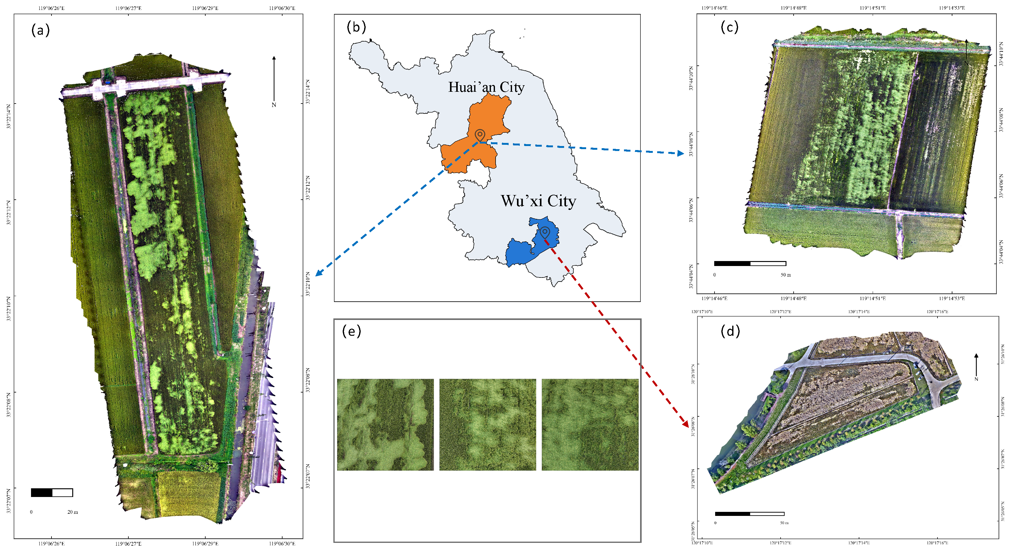
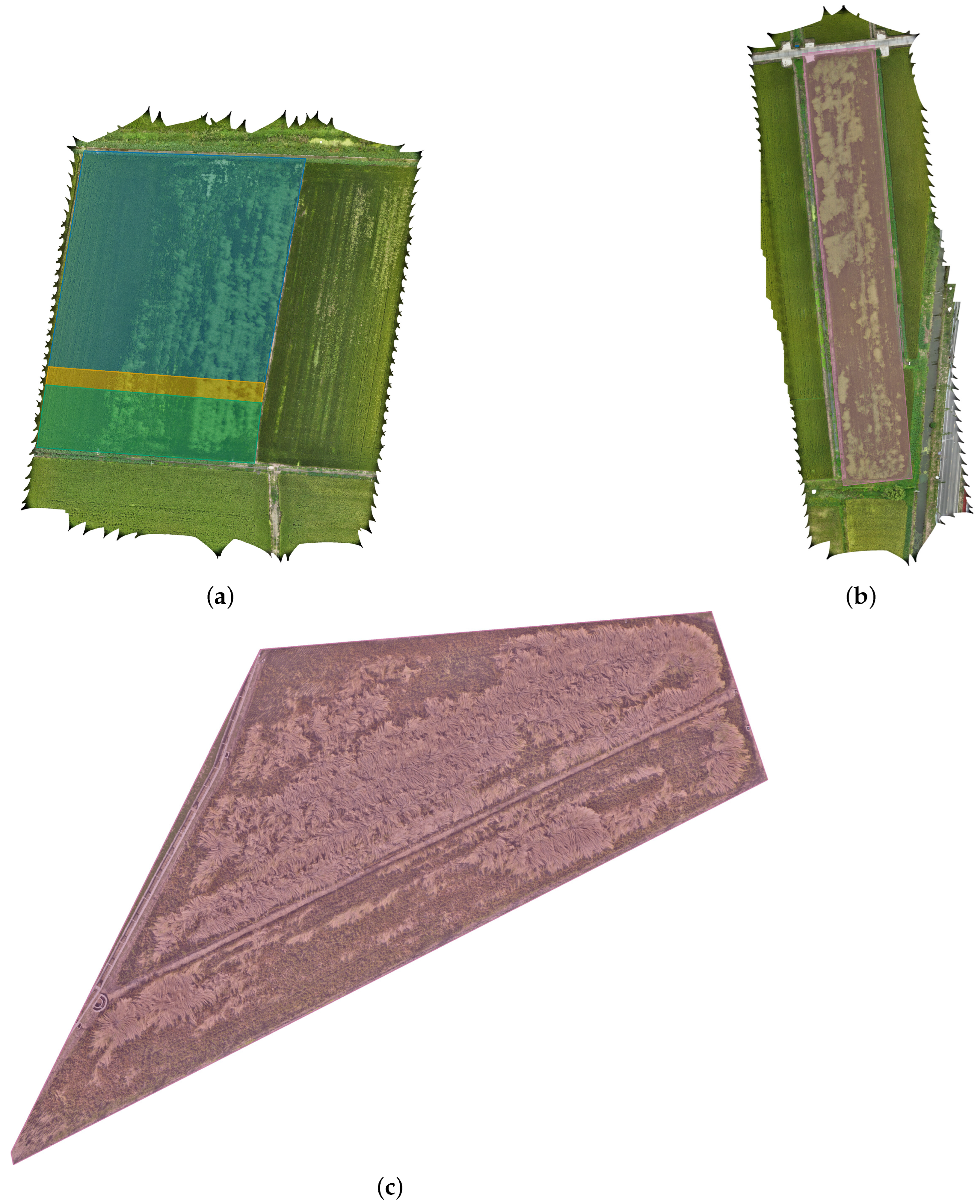
The UAV rice-lodging data comprise three parcel-level subsets collected from two rice-production regions in Jiangsu Province, China. Two parcels were acquired at Baimahu Farm, a national seed-production base in Huai’an District, Huai’an City: the 4.2 ha parcel shown in Figure 1a, denoted as HA-P1, and the 4.9 ha parcel in Figure 1c, denoted as HA-P2. Located near ${33}^{\circ }{22}^{\prime }$ N and ${119}^{\circ }{06}^{\prime }$ E on the eastern Jianghuai Plain, the farm features flat terrain suitable for large-scale rice cultivation. The region has a temperate monsoon climate, with an annual mean temperature of 13.8–14.8 °C, annual precipitation of 906–1007 mm, and approximately 2160 h of sunshine annually. Paddy soil and fluvo-aquic soil are the dominant soil types.

A third 2.7 ha parcel from Binhu District, Wuxi City, denoted as WX-P3 and shown in Figure 1d, is also included. Located near ${31}^{\circ }{26}^{\prime }$ N and ${120}^{\circ }{17}^{\prime }$ E on the northern Taihu Plain, this region has a northern subtropical humid monsoon climate, with an annual mean temperature of 15.4–16.5 °C, annual precipitation of 1050–1150 mm, and approximately 1920 h of sunshine annually. Paddy soil and fluvo-aquic soil are again the main soil types. The Huai’an parcels were imaged during the growing stage, whereas WX-P3 was imaged near harvest. Consequently, WX-P3 contains more complex backgrounds due to stronger shadow effects and more exposed soil.

Figure 1 provides an overview of the three-parcel collection: Figure 1a,c shows the global previews of HA-P1 and HA-P2, Figure 1b marks the locations of Huai’an and Wuxi within Jiangsu Province, Figure 1d shows the global preview of WX-P3, and Figure 1e presents representative lodged-rice image samples. In our evaluation protocol, HA-P2 serves as the model-development parcel, HA-P1 is the held-out Huai’an test parcel, and WX-P3 provides the external cross-region test.

UAV observations were acquired with a DJI Matrice 300 RTK platform equipped with a Zenmuse L2 LiDAR payload. The system synchronously collected RGB imagery and point-cloud data, from which co-registered orthophoto mosaics and DSM products were generated.

Table 1. Main UAV, sensor, and image-product parameters of the three-parcel UAV rice-lodging collection.

Parameter	Value
UAV platform	DJI Matrice 300 RTK
Sensor payload	Zenmuse L2 LiDAR payload with integrated RGB mapping camera
Camera sensor	CMOS
Shutter speed	1/8000–30 s
ISO range	100–12,800
Storage medium	High-speed SD card
Camera weight	Approximately 500 g
Parcel	Mosaic size/GSD
HA-P1	16,092 × 34,816 px/0.847 cm pixel−1
HA-P2	24,575 × 27,455 px/0.852 cm pixel−1
WX-P3	22,333 × 16,748 px/0.850 cm pixel−1

summarizes the main platform, sensor, flight, and image-product parameters.

2.2. RGB and DSM Preprocessing

The raw UAV observations were processed in DJI Terra to generate co-registered multimodal products. The workflow included image mosaicking, radiometric correction, color correction, spatial registration, point-cloud reconstruction, and the generation of digital orthophoto maps and DSMs. The resulting RGB images and DSMs were exported as paired .tif files to preserve georeferencing information and pixel-level alignment. This alignment is essential because the proposed framework uses DSM not only as an input modality but also as a source of geometric priors for decoder prompting, pseudo-label calibration, and boundary regularization.

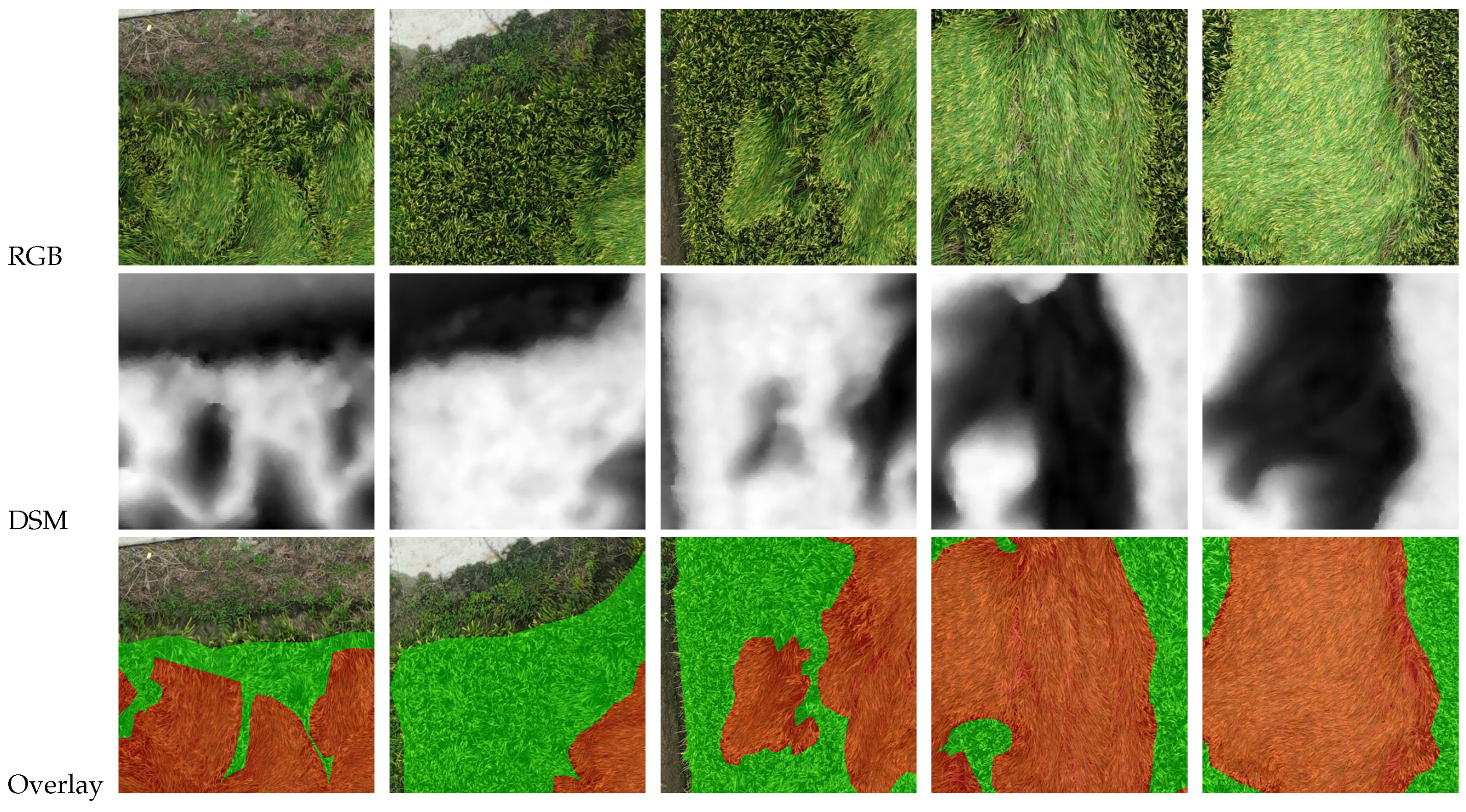
Pixel-wise annotations were produced in ArcGIS Pro 3.1 on the high-resolution orthophoto mosaics. Each pixel was assigned to one of three semantic categories: lodged rice, healthy rice, or background. Lodged rice denotes areas with visible tilting, flattening, or canopy collapse following wind, heavy rainfall, or related disturbances; these regions typically exhibit disordered texture, darker tones, and irregular canopy structure. Healthy rice denotes upright rice with normal growth, appearing as brighter and more spatially homogeneous canopy cover. Field ridges, roads, bare soil, shadows, water surfaces, weeds, and other nontarget objects were assigned to the background class.

The annotation workflow comprised three steps. First, trained annotators delineated category polygons on the georeferenced orthophoto mosaics according to the visual interpretation rules above. Second, experts in UAV agricultural image interpretation reviewed the polygon layers and verified category consistency across parcels. Third, boundary correction was performed by jointly inspecting the RGB mosaic, DSM product, and annotation layer, particularly near gradual lodging transitions, narrow ridges, shadowed areas, and mixed crop–background boundaries. The final vector annotations were rasterized to the same grid as the RGB and DSM products and exported as pixel-level label masks. Figure 2 shows representative examples.  

2.3. Parcel-Level Split and Semi-Supervised Setting

To evaluate annotation-efficient rice-lodging mapping while reducing spatial leakage, we adopted a parcel-level semi-supervised split protocol with explicit cross-scene testing. In the main HA-P2/HA-P1 benchmark, HA-P2 was used for training and validation, while HA-P1 served as the held-out in-region test parcel. The external WX-P3 parcel was reserved for direct cross-region testing. No tile from HA-P1 or WX-P3 was used for parameter updates, model selection, or hyperparameter tuning. Random tile-level splitting was avoided because neighboring UAV tiles often share similar texture, illumination, canopy structure, and height patterns, which can lead to overly optimistic accuracy estimates.

Appendix A provides spatial partition maps with semi-transparent overlays for all three parcels, complementing Figure 1 and allowing readers to inspect the spatial separation among the HA-P2 model-development regions, the HA-P1 in-region test parcel, and the WX-P3 external test parcel.

For the main benchmark, HA-P2 was first divided into spatially contiguous training and validation regions. All parcels were then synchronously cropped into $512\times 512$ pixel RGB and DSM tiles. Tiles with large blank regions, insufficient valid content, or poor image quality were removed. The main benchmark contains approximately 1400 high-quality paired tiles, and the external WX-P3 set contributes 300 additional fully annotated paired tiles for direct cross-region testing. Under the semi-supervised setting, only 10%, 20%, or 40% of the HA-P2 training tiles retained pixel-level annotations, while the remaining training tiles were used as unlabeled data. The validation set was used for model selection and hyperparameter tuning but not for parameter updates. The HA-P1 test set was fixed across all labeled ratios and used only for final evaluation. Unless otherwise stated, each experiment was repeated three times with different labeled and unlabeled splits using seeds 0, 1, and 2, and the mean performance is reported.

To further examine cross-region generalization, we directly evaluated the 40% labeled HA-P2-source models on WX-P3. All training, validation, and model-selection operations remained confined to HA-P2; WX-P3 was used only for final testing and was not involved in parameter updates or hyperparameter tuning. The WX-P3 results are reported in Section 4.4.

This protocol defines the learning problem considered in the following Section 3. The labeled set is denoted as

$${\mathcal{D}}_l={\left\{\left({\mathbf{x}}_i^r,{\mathbf{x}}_i^d,{\mathbf{y}}_i\right)\right\}}_{i=1}^{N_l},$$

(1)

where ${\mathbf{x}}_i^r\in {\mathbb{R}}^{H\times W\times 3}$ is the RGB tile, ${\mathbf{x}}_i^d\in {\mathbb{R}}^{H\times W\times 1}$ is the aligned DSM tile, and ${\mathbf{y}}_i\in {\{1,\dots ,C\}}^{H\times W}$ is the pixel-level annotation. The unlabeled set is denoted as

$${\mathcal{D}}_u={\left\{\left({\mathbf{x}}_j^r,{\mathbf{x}}_j^d\right)\right\}}_{j=1}^{N_u}.$$

(2)

GUMatch uses paired RGB and DSM inputs in both sets. The labels in ${\mathcal{D}}_l$ provide supervised category learning, whereas the unlabeled pairs in ${\mathcal{D}}_u$ are used to construct geometry-guided pseudo-label supervision during teacher–student training.

3. Method

To improve readability, we use bold uppercase symbols for image-level maps or tensors and lower-case indexed symbols for their pixel values, e.g., $\mathbf{U}$ and $u_i$. Algorithms 1 and 2 use the same map-level symbols as the corresponding formulas. The main abbreviations and symbols are also summarized in the “Abbreviations and Symbols” section at the end of the paper.

3.1. Framework Overview

Figure 3 compares UniMatch V2 with the proposed GUMatch. UniMatch V2 [29] employs an EMA teacher–student framework with weak-to-strong consistency. The teacher generates pseudo-labels from a weakly augmented view, while the student learns from two strong views derived from the same image. Complementary channel-wise dropout is applied to strong-view features before decoding, enabling the same weak-view supervision to regularize both streams. GUMatch retains this effective optimization scaffold but introduces a DSM encoder, a DSM edge prior, reliability-aware decoder prompting, geometry-calibrated pseudo-label weights, and a boundary regularizer. These components allow DSM evidence to guide both feature decoding and teacher–student supervision.

Unlike supervised RGB–DSM segmentation networks such as CMGFNet and LMFNet, which learn cross-modal feature interaction from densely labeled data, GUMatch focuses on unlabeled RGB–DSM pairs and explicitly assesses whether DSM evidence should be trusted before modifying decoder features or pseudo-label supervision. This distinction is critical for UAV rice-lodging scenes, where photogrammetric DSMs may contain local noise, voids, and residual mis-registration.

The data flow in GUMatch links AGP, GPL, and BGR through a shared DSM edge prior. For each RGB–DSM branch, the DSM encoder produces a prompt pyramid and an edge-prior map. AGP uses these signals to gate the RGB decoder features. On the weak view, the teacher prediction provides pseudo-labels, confidence scores, and a semantic boundary response. GPL combines these teacher outputs with the DSM edge prior to generate calibrated confidence weights, valid pseudo-label masks, and boundary bands in weak-view coordinates. The same geometric transformations then transfer these targets and the DSM edge prior to the two strong views. BGR is applied to the strong-view student predictions only within the transferred valid boundary regions. Thus, the edge prior flows from decoder prompting to pseudo-label calibration and boundary regularization, while GPL controls where the boundary loss is permitted to act.

During weak-to-strong training, strong appearance perturbations are applied only to RGB, whereas DSM follows synchronized geometric transformations to preserve height meaning and RGB–DSM alignment. GUMatch uses paired RGB–DSM inputs during both training and inference, so the DSM branch is not merely a training-only auxiliary module. AGP requires DSM to produce gated decoder features, and the geometry-guided losses use DSM to define boundary-risk and edge-prior signals during training.

3.2. Adaptive Geometric Prompting Module

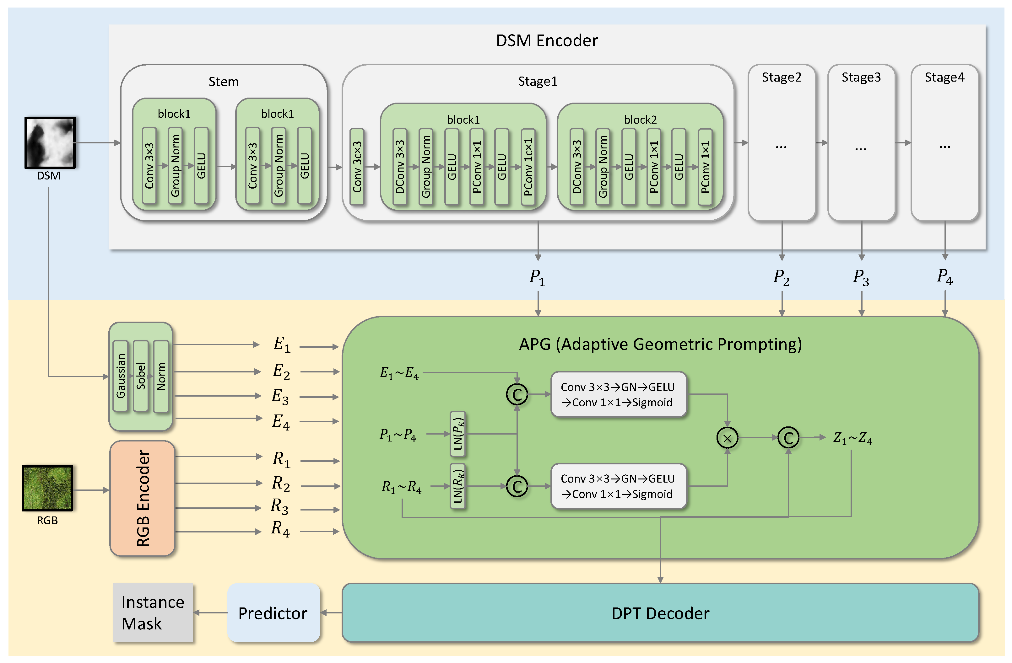
AGP transforms DSM from an auxiliary input into a structured geometric prior through a selective three-stage design: multiscale DSM prompt construction, edge-prior extraction, and reliability-aware prompt gating. This design mitigates the risk of uniformly injecting DSM features into the decoder when DSMs contain reconstruction noise, local voids, or mis-registration. Figure 4 provides the network-level view. For branch ★, the DSM branch produces the prompt pyramid ${\left\{{\mathbf{P}}_k^{★}\right\}}_{k=1}^K$, the geometric branch derives the edge prior ${\mathbf{E}}^{d,★}$, and scale matching supplies ${\mathrm{\Gamma }}_k\left({\mathbf{E}}^{d,★}\right)$ to the gate. AGP then combines these terms with the RGB decoder feature ${\overline{\mathbf{F}}}_k^{r,★}$ to compute the gated residual correction before DPT decoding.

3.2.1. DSM Encoder

RGB imagery and DSM provide complementary but fundamentally different evidence: RGB primarily contributes semantic appearance, whereas DSM captures local elevation changes and surface discontinuities. We therefore adopt an asymmetric dual-encoder design. Let $g_r$ and $g_d$ denote the RGB and DSM encoders, respectively. For branch ★, which denotes a labeled, weak, or strong view, multiscale features are extracted as

$${\left\{{\mathbf{F}}_k^{r,★}\right\}}_{k=1}^K=g_r\left({{\mathbf{x}}^r}^{★}\right),{\left\{{\mathbf{F}}_k^{d,★}\right\}}_{k=1}^K=g_d\left({{\mathbf{x}}^d}^{★}\right),{\mathbf{P}}_k^{★}={\varphi }_k\left({\mathbf{F}}_k^{d,★}\right),$$

(3)

where $K=4$ in our implementation. The RGB encoder $g_r$ is instantiated by DINOv2 [31], and $g_d$ is a lightweight hierarchical convolutional encoder. The projection ${\varphi }_k(·)$ maps DSM features to the decoder channel dimension, so ${\mathbf{P}}_k^{★}$ acts as a scale-aligned carrier of geometric evidence rather than as a second semantic stream.  

3.2.2. DSM Edge Prior Construction

AGP also extracts a class-agnostic DSM edge prior as the shared geometric reference for prompt gating, GPL, and BGR. Because raw DSM gradients may contain large local outliers from reconstruction artifacts, we define a robust normalization operator for any nonnegative response map $\mathbf{X}\in {\mathbb{R}}_{\ge 0}^{H\times W}$:

$$\mathrm{Norm}\left(\mathbf{X}\right)=1-exp\left(-{\displaystyle \frac{\mathbf{X}}{\frac{1}{\left|\mathrm{\Omega }\right|}{\sum }_{i\in \mathrm{\Omega }}{X}_i+{ϵ}_n}}\right),$$

(4)

where $\mathrm{\Omega }$ is the pixel set and ${ϵ}_n>0$ prevents division by zero. Equation (4) scales responses by the image-wide average magnitude and saturates smoothly, making it less sensitive to isolated DSM artifacts or spurious prediction gradients than max-based normalization. The class-agnostic DSM edge-magnitude map is then

$${\overline{\mathbf{E}}}^d\left({\mathbf{x}}^d\right)=\sqrt{{\left(K_x\ast ({\mathcal{G}}_{\sigma }\ast {\mathbf{x}}^d)\right)}^2+{\left(K_y\ast ({\mathcal{G}}_{\sigma }\ast {\mathbf{x}}^d)\right)}^2},$$

(5)

where $K_x,K_y$ are Sobel kernels, ${\mathcal{G}}_{\sigma }$ is Gaussian smoothing, and ∗ denotes convolution. For the labeled and weak branches, Equation (4) gives ${\mathbf{E}}^{d,l}$ and ${\mathbf{E}}^{d,w}$ from ${\overline{\mathbf{E}}}^{d,l}={\overline{\mathbf{E}}}^d\left({{\mathbf{x}}^d}^l\right)$ and ${\overline{\mathbf{E}}}^{d,w}={\overline{\mathbf{E}}}^d\left({{\mathbf{x}}^d}^w\right)$. For the strong branches, we transform the raw weak-view edge magnitude before normalization to avoid CutMix-induced artificial edges:

$${\overline{\mathbf{E}}}^{d,s,v}={\mathcal{T}}^v\left({\overline{\mathbf{E}}}^{d,w}\right),{\mathbf{E}}^{d,s,v}=\mathrm{Norm}\left({\overline{\mathbf{E}}}^{d,s,v}\right),v\in \{1,2\}.$$

(6)

When CutMix pastes a region from another unlabeled sample, the paired raw edge magnitude is pasted into the same region before normalization, ensuring that ${\mathbf{E}}^{d,s,v}$ remains tied to scene geometry rather than augmentation artifacts.

3.2.3. Reliability-Aware Prompt Gating and Decoder Injection

Given the prompt features and edge prior, AGP estimates where DSM should influence decoding. Let ${\overline{\mathbf{F}}}_k^{r,★}$ be the RGB feature entering AGP; it equals the raw RGB feature on the labeled and weak branches and the complementary-dropout feature on the strong branches (Section 3.3.1). The spatial gate is

$${\mathbf{Q}}_k^{★}=\underset{\mathrm{response}\mathrm{term}}{\underbrace{\sigma \left({\psi }_k^r\left(\left[\mathrm{LN}\left({\mathbf{P}}_k^{★}\right);{\mathrm{\Gamma }}_k\left({\mathbf{E}}^{d,★}\right)\right]\right)\right)}}\odot \underset{\mathrm{compatibility}\mathrm{term}}{\underbrace{\sigma \left({\psi }_k^c\left(\left[\mathrm{LN}\left({\overline{\mathbf{F}}}_k^{r,★}\right);\mathrm{LN}\left({\mathbf{P}}_k^{★}\right)\right]\right)\right)}},$$

(7)

where ${\mathrm{\Gamma }}_k(·)$ is scale matching, $\mathrm{LN}(·)$ is feature normalization, and ${\psi }_k^r,{\psi }_k^c$ are lightweight convolutional predictors. The first term measures intrinsic geometric reliability, and the second term measures RGB–DSM compatibility. Both terms are single-channel spatial maps broadcast along feature channels.

At scale k, the DPT decoder consumes the fused feature

$${\mathbf{Z}}_k^{★}={\overline{\mathbf{F}}}_k^{r,★}+{\lambda }_k{\mathbf{Q}}_k^{★}\odot {\mathbf{P}}_k^{★},$$

(8)

where ${\lambda }_k$ is a learnable scale-specific coefficient. The residual formulation preserves RGB as the primary semantic carrier and allows DSM to contribute only through a gated correction. We denote the complete segmentation network as $f_{\theta }({{\mathbf{x}}^r}^{★},{{\mathbf{x}}^d}^{★};{\mathbf{E}}^{d,★})$.

3.3. Geometry-Guided Semi-Supervised Optimization

After AGP establishes the shared geometric prior, unlabeled training must use it without corrupting the physical meaning of DSM. GUMatch achieves this through a modality-preserving weak-to-strong protocol, geometry-calibrated pseudo-label supervision, and a conservative boundary refinement loss.

3.3.1. Modality-Preserving Weak-to-Strong Training Protocol

Weak-to-strong semi-supervised learning requires strong student perturbations, but RGB–DSM training must preserve DSM height meaning. For each unlabeled sample $({\mathbf{x}}^r,{\mathbf{x}}^d)\in {\mathcal{D}}_u$, we first build a weak teacher view $({{\mathbf{x}}^r}^w,{{\mathbf{x}}^d}^w)={\mathcal{A}}_w({\mathbf{x}}^r,{\mathbf{x}}^d)$, where ${\mathcal{A}}_w$ comprises geometry-preserving resize, crop, and horizontal flip shared by RGB and DSM. Two student strong views are derived as

$${{\mathbf{x}}^r}^{s,v}={\mathcal{A}}_{app}^v\left({\mathcal{T}}^v\left({{\mathbf{x}}^r}^w\right)\right),{{\mathbf{x}}^d}^{s,v}={\mathcal{T}}^v\left({{\mathbf{x}}^d}^w\right),v\in \{1,2\},$$

(9)

where ${\mathcal{A}}_{app}^v$ is RGB-only appearance perturbation and ${\mathcal{T}}^v$ is the synchronized spatial transform, primarily CutMix in our implementation. This asymmetric protocol perturbs RGB appearance while keeping DSM photometrically unchanged; we refer to it as ASV in the ablation study.

We retain complementary dropout only on the RGB strong-view features. To avoid conflict with the pseudo-label valid mask $\mathbf{M}$ used in GPL, the channel-wise dropout masks are denoted by ${\Delta }_1$ and ${\Delta }_2$, with ${\Delta }_1,{\Delta }_2\in {\{0,2\}}^{C\times 1\times 1}$ and ${\Delta }_1+{\Delta }_2=2\mathbf{1}$. The same mask pair is shared across all selected RGB backbone scales:

$${\overline{\mathbf{F}}}_k^{r,s,1}={\Delta }_1\odot {\mathbf{F}}_k^{r,s,1},{\overline{\mathbf{F}}}_k^{r,s,2}={\Delta }_2\odot {\mathbf{F}}_k^{r,s,2},$$

(10)

For the weak teacher and labeled branches, complementary dropout is disabled, so ${\overline{\mathbf{F}}}_k^{r,w}={\mathbf{F}}_k^{r,w}$ and ${\overline{\mathbf{F}}}_k^{r,l}={\mathbf{F}}_k^{r,l}$. DSM prompt features ${\mathbf{P}}_k^{★}$ are never masked.

3.3.2. Geometry-Calibrated Pseudo-Label Supervision

In lodging scenes, the teacher’s most harmful errors typically arise near ambiguous boundaries, where RGB appearance is weakly discriminative but supervision decisions carry high geometric consequence. GPL therefore does not alter the teacher’s semantic prediction itself; instead, it regulates how much each pseudo-label should be trusted, with geometry-guided down-weighting activated only within teacher-identified boundary-risk regions.

The student and teacher networks are parameterized by $\theta$ and ${\theta }^{\prime }$, respectively, with ${\theta }^{\prime }$ updated as the EMA of $\theta$ with momentum $\eta \in (0,1)$. On the weak view $({{\mathbf{x}}^r}^w,{{\mathbf{x}}^d}^w)$, the teacher produces logits ${\mathbf{z}}_t^w=f_{{\theta }^{\prime }}({{\mathbf{x}}^r}^w,{{\mathbf{x}}^d}^w;{\mathbf{E}}^{d,w})$ and probabilities ${\mathbf{p}}^w=\mathrm{softmax}\left({\mathbf{z}}_t^w\right)$. For each pixel i, the pseudo-label is ${\widehat{y}}_i=arg{max}_c{{\mathbf{p}}^w}_{i,c}$ and the raw confidence is $s_i={max}_c{{\mathbf{p}}^w}_{i,c}$. The corresponding map-level symbols used in Algorithm 1 are $\widehat{\mathbf{Y}}$ and $\mathbf{S}$. To localize where calibration is needed, we derive the teacher boundary response

$${\mathbf{B}}^w=\mathrm{Norm}\left({\displaystyle \sum _{c=1}^C}\sqrt{{\left(K_x\ast {{\mathbf{p}}^w}^{\left(c\right)}\right)}^2+{\left(K_y\ast {{\mathbf{p}}^w}^{\left(c\right)}\right)}^2}\right),$$

(11)

and activate calibration only within the teacher-derived boundary band

$$u_i=\mathbb{I}\left({\left({MaxPool}_{r_b}\left({\mathbf{B}}^w\right)\right)}_i>{\tau }_b\right),$$

(12)

where ${MaxPool}_{r_b}(·)$ is max pooling with radius $r_b$ and ${\tau }_b$ controls the band width. The semantic-geometric agreement is

$$a_i=(1-u_i)+u_{i}exp\left(-{\displaystyle \frac{\left|{\mathbf{B}}_i^w-{\mathbf{E}}_i^{d,w}\right|}{{\tau }_g}}\right),$$

(13)

where ${\tau }_g>0$ controls the tolerance to RGB–DSM boundary mismatch. As $a_i=1$ outside the boundary band, nonboundary pixels are not penalized. The calibrated confidence is

$${\tilde{c}}_i=s_i\left(1-(1-\alpha )u_i(1-a_i)\right),$$

(14)

where $\alpha \in [0,1]$ controls the down-weighting strength. The factor in Equation (14) lies in $[\alpha ,1]$, so geometry can suppress but never inflate teacher confidence. The valid pseudo-label mask is $m_i=\mathbb{I}({\tilde{c}}_i\ge {\tau }_c)$.

The map-level targets $\widehat{\mathbf{Y}}$, $\tilde{\mathbf{C}}$, $\mathbf{M}$, and $\mathbf{U}$ are generated in weak-view coordinates and transferred to each strong branch by the same ${\mathcal{T}}^v$ used in Equation (9); ${\mathbf{E}}^{d,s,v}$ follows Equation (6). Discrete targets use nearest-neighbor transformation, whereas continuous confidence and edge maps use bilinear interpolation before CutMix pasting. Algorithm 1 summarizes this calibration-and-transfer procedure with symbols matched to Equations (11)–(14).

Given the transformed teacher targets, the student produces strong-view logits ${\mathbf{z}}^{s,v}=f_{\theta }\left({{\mathbf{x}}^r}^{s,v},{{\mathbf{x}}^d}^{s,v};{\mathbf{E}}^{d,s,v}\right)$ and probabilities ${\mathbf{p}}^{s,v}=\mathrm{softmax}\left({\mathbf{z}}^{s,v}\right)$ for $v\in \{1,2\}$. The resulting per-view unsupervised loss is a confidence-weighted cross-entropy:

$${\mathcal{L}}_u^v={\displaystyle \frac{{\sum }_i{M}_i^v{\tilde{C}}_i^v\mathrm{CE}\left({\mathbf{z}}_i^{s,v},{\widehat{Y}}_i^v\right)}{{\sum }_i{M}_i^v{\tilde{C}}_i^v+ϵ}},v\in \{1,2\},$$

(15)

where $\mathrm{CE}(·,·)$ is pixel-wise cross-entropy and $ϵ$ prevents division by zero. The final unlabeled objective averages the two strong views, ${\mathcal{L}}_u=\frac{1}{2}({\mathcal{L}}_u^1+{\mathcal{L}}_u^2)$. Equation (15) maintains the weak-to-strong consistency principle of UniMatch V2 while employing modality-preserving strong views and geometry-calibrated pseudo-label weights. RGB is optimized for appearance robustness, whereas DSM remains a stable geometric condition across the two strong branches.  

Algorithm 1 GPL target generation and transfer with formula-matched notation

Input:  weak view $({{\mathbf{x}}^r}^w,{{\mathbf{x}}^d}^w)$, weak-view DSM prior ${\mathbf{E}}^{d,w}$ Input:  EMA teacher $f_{{\theta }^{\prime }}$, strong-view operators ${\left\{{\mathcal{T}}^v\right\}}_{v=1}^2$ Output:  transformed targets ${\{{\widehat{\mathbf{Y}}}^v,{\tilde{\mathbf{C}}}^v,{\mathbf{M}}^v,{\mathbf{U}}^v\}}_{v=1}^2$   1: ${\mathbf{z}}_t^w\leftarrow f_{{\theta }^{\prime }}\left({{\mathbf{x}}^r}^w,{{\mathbf{x}}^d}^w;{\mathbf{E}}^{d,w}\right)$ and ${\mathbf{p}}^w\leftarrow \mathrm{softmax}\left({\mathbf{z}}_t^w\right)$   2: $\widehat{\mathbf{Y}}\leftarrow arg{max}_c{\mathbf{p}}^w$ and $\mathbf{S}\leftarrow {max}_c{\mathbf{p}}^w$                                  ▹ map forms of ${\widehat{y}}_i$ and $s_i$   3: Compute teacher boundary response ${\mathbf{B}}^w$ by Equation (11)   4: Compute boundary-band indicator $\mathbf{U}$ by Equation (12)   5: Compute geometry agreement $\mathbf{A}$ by Equation (13)   6: Compute calibrated confidence $\tilde{\mathbf{C}}$ from $\mathbf{S}$, $\mathbf{U}$, and $\mathbf{A}$ by Equation (14)   7: $\mathbf{M}\leftarrow \mathbb{I}\left(\tilde{\mathbf{C}}\ge {\tau }_c\right)$   8: for  $v\in \{1,2\}$  do   9:        ${\widehat{\mathbf{Y}}}^v\leftarrow {\mathcal{T}}^v\left(\widehat{\mathbf{Y}}\right)$ and ${\tilde{\mathbf{C}}}^v\leftarrow {\mathcal{T}}^v\left(\tilde{\mathbf{C}}\right)$ 10:       ${\mathbf{M}}^v\leftarrow {\mathcal{T}}^v\left(\mathbf{M}\right)$ and ${\mathbf{U}}^v\leftarrow {\mathcal{T}}^v\left(\mathbf{U}\right)$ 11: return ${\{{\widehat{\mathbf{Y}}}^v,{\tilde{\mathbf{C}}}^v,{\mathbf{M}}^v,{\mathbf{U}}^v\}}_{v=1}^2$

3.3.3. Boundary-Aware Geometric Regularization

GPL improves pseudo-label reliability, but the supervision remains primarily category-level and does not directly constrain boundary shape. We therefore add BGR as a conservative refinement loss atop GPL-filtered supervision. It avoids global alignment to all DSM edges, as field ridges, tractor ruts, and drainage channels can create strong height discontinuities unrelated to lodging boundaries.

For each strong view, the student boundary response is extracted from the soft prediction analogously to Equation (11):

$${\widehat{\mathbf{B}}}^{s,v}=\mathrm{Norm}\left({\displaystyle \sum _{c=1}^C}\sqrt{{\left(K_x\ast {\mathbf{p}}^{s,v,\left(c\right)}\right)}^2+{\left(K_y\ast {\mathbf{p}}^{s,v,\left(c\right)}\right)}^2}\right),v\in \{1,2\},$$

(16)

Using the transformed DSM prior ${\mathbf{E}}^{d,s,v}$ from Equation (6), BGR activates boundary supervision only at the intersection of valid pseudo-labels, boundary candidates, and nontrivial DSM edges:

$${\mathbf{M}}_b^v=\underset{\mathrm{valid}\mathrm{pseudo}‐\mathrm{label}}{\underbrace{{\mathbf{M}}^v}}\odot \underset{\mathrm{boundary}\mathrm{candidate}}{\underbrace{{\mathbf{U}}^v}}\odot \underset{\mathrm{nontrivial}\mathrm{DSM}\mathrm{edge}}{\underbrace{\mathbb{I}\left({\mathbf{E}}^{d,s,v}>{\tau }_d\right)}},v\in \{1,2\},$$

(17)

where ${\tau }_d$ is the DSM-edge threshold. The per-view boundary regularization loss is

$${\mathcal{L}}_{edge}^v={\displaystyle \frac{{\sum }_i{M}_{b,i}^v{\tilde{C}}_i^v\left|{\widehat{B}}_i^{s,v}-E_i^{d,s,v}\right|}{{\sum }_i{M}_{b,i}^v{\tilde{C}}_i^v+ϵ}},v\in \{1,2\},$$

(18)

and the overall boundary regularizer averages the two strong views:

$${\mathcal{L}}_{edge}=\frac{1}{2}\left({\mathcal{L}}_{edge}^1+{\mathcal{L}}_{edge}^2\right).$$

(19)

Thus, Equation (18) refines GPL-filtered supervision only where pseudo-labels and DSM evidence are jointly reliable.

Here, ${\widehat{\mathbf{B}}}^{s,v}$ is a semantic-boundary response, whereas ${\mathbf{E}}^{d,s,v}$ is a DSM height-discontinuity response. We use L1 amplitude matching because Equation (4) puts the two responses into a comparable dynamic range under the mask in Equation (17). Alternatives such as Dice on binarized maps or active-contour-style losses [32] were less stable in our experiments, as they may lose useful gradients on weak boundaries or fit noisy DSM ridges too aggressively. reports the empirical comparison.

3.4. Supervised Loss and Overall Objective

For labeled samples, the student predicts logits ${\mathbf{z}}^l=f_{\theta }\left({{\mathbf{x}}^r}^l,{{\mathbf{x}}^d}^l;{\mathbf{E}}^{d,l}\right)$, and the supervised loss is the standard pixel-wise cross-entropy:

$${\mathcal{L}}_{sup}={\displaystyle \frac{1}{\left|\mathrm{\Omega }\right|}}\sum _{i\in \mathrm{\Omega }}\mathrm{CE}\left({\mathbf{z}}_i^l,y_i\right),$$

(20)

over the labeled pixel set $\mathrm{\Omega }$. The overall training objective combines the supervised loss with the two unsupervised components:

$$\mathcal{L}={\mathcal{L}}_{sup}+{\lambda }_u{\mathcal{L}}_u+{\lambda }_e{\mathcal{L}}_{edge},$$

(21)

where ${\lambda }_u$ and ${\lambda }_e$ balance the two unsupervised terms. The teacher parameters are updated as the EMA of the student with momentum $\eta$. Algorithm 2 summarizes the full training routine and references the equations used in each step.  

Algorithm 2 Overall training procedure of GUMatch

Input:  labeled set ${\mathcal{D}}_l$, unlabeled set ${\mathcal{D}}_u$ Input:  student $f_{\theta }$, EMA teacher $f_{{\theta }^{\prime }}$, weak augmentation ${\mathcal{A}}_w$ Input:  strong-view operators ${\{{\mathcal{A}}_{app}^v,{\mathcal{T}}^v\}}_{v=1}^2$, ${\lambda }_u$, ${\lambda }_e$, $\eta$ Output:  trained student $\theta$ and teacher ${\theta }^{\prime }$   1: Initialize ${\theta }^{\prime }\leftarrow \theta$   2: for each training iteration do   3:      Sample $({{\mathbf{x}}^r}^l,{{\mathbf{x}}^d}^l,{\mathbf{Y}}^l)\sim {\mathcal{D}}_l$ and $({\mathbf{x}}^r,{\mathbf{x}}^d)\sim {\mathcal{D}}_u$   4:      $({{\mathbf{x}}^r}^w,{{\mathbf{x}}^d}^w)\leftarrow {\mathcal{A}}_w({\mathbf{x}}^r,{\mathbf{x}}^d)$   5:      Compute ${\overline{\mathbf{E}}}^{d,l},{\overline{\mathbf{E}}}^{d,w}$ by Equation (5) and ${\mathbf{E}}^{d,l},{\mathbf{E}}^{d,w}$ by Equation (4)   6:      for $v\in \{1,2\}$ do   7:           Generate $({{\mathbf{x}}^r}^{s,v},{{\mathbf{x}}^d}^{s,v})$ by Equation (9)   8:           Generate ${\mathbf{E}}^{d,s,v}$ by Equation (6)   9:      $$\begin{gathered} ({\widehat{\mathbf{Y}}}^1,{\tilde{\mathbf{C}}}^1,{\mathbf{M}}^1,{\mathbf{U}}^1,{\widehat{\mathbf{Y}}}^2,{\tilde{\mathbf{C}}}^2,{\mathbf{M}}^2,{\mathbf{U}}^2) \\ \leftarrow {\mathrm{GPL}}_{\mathrm{TARGETS}}({{\mathbf{x}}^r}^w,{{\mathbf{x}}^d}^w,{\mathbf{E}}^{d,w},f_{{\theta }^{\prime }},{\left\{{\mathcal{T}}^v\right\}}_{v=1}^2) \end{gathered}$$ 10:      for $v\in \{1,2\}$ do 11:           ${\mathbf{z}}^{s,v}\leftarrow f_{\theta }\left({{\mathbf{x}}^r}^{s,v},{{\mathbf{x}}^d}^{s,v};{\mathbf{E}}^{d,s,v}\right)$ 12:           Compute ${\mathcal{L}}_u^v$ by Equation (15) and ${\mathcal{L}}_{edge}^v$ by Equation (18) 13:      ${\mathbf{z}}^l\leftarrow f_{\theta }\left({{\mathbf{x}}^r}^l,{{\mathbf{x}}^d}^l;{\mathbf{E}}^{d,l}\right)$ and compute ${\mathcal{L}}_{sup}$ 14:      ${\mathcal{L}}_u\leftarrow ({\mathcal{L}}_u^1+{\mathcal{L}}_u^2)/2$ and ${\mathcal{L}}_{edge}\leftarrow ({\mathcal{L}}_{edge}^1+{\mathcal{L}}_{edge}^2)/2$ 15:      Compute $\mathcal{L}$ by Equation (21) 16:      Update $\theta$ by back-propagating $\mathcal{L}$ 17:      Update ${\theta }^{\prime }\leftarrow \eta {\theta }^{\prime }+(1-\eta )\theta$ 18: return  $\theta ,{\theta }^{\prime }$

4. Experimental Results and Analysis

4.1. Experimental Setting

All experiments were run on Ubuntu 20.04 using Python 3.11.9, PyTorch 2.5.0, and CUDA 12.4 under Miniconda. The workstation contained an Intel Xeon 8360Y CPU (2.40 GHz) and one NVIDIA RTX 3090 GPU (24 GB).

Following the parcel-level protocol in Section 2, the main HA-P2/HA-P1 benchmark contained 1400 RGB–DSM tiles: 900 training tiles from HA-P2, 200 validation tiles from HA-P2, and 300 in-region test tiles from HA-P1. The external WX-P3 set contained 300 fully annotated tiles and was used only for direct cross-region testing. All models were trained and selected only on HA-P2; HA-P1 and WX-P3 were used only as final test parcels.

The labeled ratios were applied only to the HA-P2 training set: 10%, 20%, and 40% correspond to 90, 180, and 360 labeled tiles, respectively, with the remaining training tiles used as unlabeled data. Inputs were cropped to $512\times 512$, and all models were trained for 200 epochs. Each iteration drew one labeled mini-batch and one unlabeled mini-batch, each with batch size 2. Validation and testing used batch size 1. Weak augmentation applied synchronized random resize, random crop, and horizontal flip to RGB and DSM. Strong student views further applied RGB-only color jitter, grayscale conversion, Gaussian blur, and CutMix (probability 0.5), while DSM retained only the same geometric transforms to preserve height structure.

We used AdamW (${\beta }_1=0.9$, ${\beta }_2=0.999$, weight decay 0.01). For DINOv2-B, the pretrained RGB backbone used an initial learning rate of $5\times {10}^{-6}$; the decoder, DSM encoder, AGP module, and other newly initialized layers used a $40\times$ multiplier. We adopted a polynomial decay schedule, $l{r}_t=l{r}_0{(1-t/T)}^{0.9}$, with t and T the current and total iterations. DINOv2-B was initialized from the official checkpoint, and RN-101 from ImageNet weights; the DSM encoder, AGP module, and task-specific decoder layers were randomly initialized. The pseudo-label confidence threshold was ${\tau }_c=0.85$. The unsupervised consistency and boundary regularization weights were ${\lambda }_u=1.0$ and ${\lambda }_e=0.5$. The EMA teacher momentum was updated as ${\eta }_t=min(1-1/(t+1),0.996)$. For GPL and BGR, we set $r_b=3$, ${\tau }_b=0.2$, ${\tau }_g=0.25$, $\alpha =0.40$, and ${\tau }_d=0.2$. Each setting was repeated with seeds 0, 1, and 2, and we report the mean. For the seed-matched method comparisons in

Table 2. mIoU (%) results on the HA-P2→HA-P1 in-region benchmark. Each cell is the mean ± standard deviation over three independent labeled/unlabeled splits with seeds 0, 1, and 2. ^† denotes fully supervised methods retrained on the same labeled subsets to provide a multimodal reference under scarce labels. Panel A reports the RN-101 benchmark and RGB–DSM references, panel B reports multimodal semi-supervised baselines, and panel C reports the DINOv2-B variants.

Method	Encoder	10% Labels	20% Labels	40% Labels
Panel A. RN-101 Benchmark and RGB–DSM References
Labeled Only	RN-101	71.62 ± 0.31	75.48 ± 0.27	78.96 ± 0.22
ST++ [33]	RN-101	75.88 ± 0.26	78.92 ± 0.21	81.24 ± 0.18
PS-MT [34]	RN-101	75.41 ± 0.24	78.55 ± 0.20	81.47 ± 0.16
UniMatch V1 [28]	RN-101	77.03 ± 0.22	79.84 ± 0.18	82.36 ± 0.15
DAW [35]	RN-101	76.84 ± 0.21	80.02 ± 0.20	82.28 ± 0.16
CorrMatch [36]	RN-101	77.46 ± 0.20	80.38 ± 0.18	82.54 ± 0.14
UniMatch V2 [29]	RN-101	77.82 ± 0.18	80.76 ± 0.16	82.93 ± 0.13
RSProtoSemiSeg [30]	RN-101	78.41 ± 0.19	81.18 ± 0.17	83.39 ± 0.14
Multimodal RGB–DSM baselines
CMGFNet † [22]	RN-101	76.92 ± 0.25	80.21 ± 0.20	82.74 ± 0.16
LMFNet † [24]	RN-101	77.45 ± 0.22	80.74 ± 0.19	83.08 ± 0.15
UniMatch V2 + DSM (early concat)	RN-101	78.34 ± 0.20	81.07 ± 0.18	83.21 ± 0.15
UniMatch V2 + DSM (decoder add)	RN-101	78.61 ± 0.19	81.25 ± 0.17	83.46 ± 0.15
GUMatch	RN-101	80.12 ± 0.18	82.98 ± 0.15	85.06 ± 0.13
Panel B. Multimodal Semi-Supervised Baselines
M3L [37]	MiT-B4	78.90 ± 0.21	81.88 ± 0.18	84.05 ± 0.17
DepMatch [38]	DINOv2-B	80.55 ± 0.14	81.49 ± 0.16	84.31 ± 0.13
Panel C. Backbone Upgrade with DINOv2-B
UniMatch V2 [29]	DINOv2-B	80.35 ± 0.16	82.54 ± 0.14	84.44 ± 0.12
UniMatch V2 + DSM (decoder add)	DINOv2-B	81.18 ± 0.15	83.21 ± 0.13	84.97 ± 0.12
GUMatch	DINOv2-B	82.64 ± 0.14	84.95 ± 0.13	86.72 ± 0.11

, we used a paired nonparametric sign test.

4.2. Evaluation Metrics

We adopt mean intersection over union (mIoU) as the primary metric and report class-wise IoU for per-category analysis. All metrics are computed on the corresponding fixed test parcel over three classes: lodged rice, healthy rice, and background. As lodging boundaries are often gradual and spatially ambiguous, we further report the boundary F1-score (BF1) in the ablation and robustness analyses. We extract class-agnostic boundaries from the predicted and ground-truth maps and count a boundary pixel as matched if it lies within a small tolerance band of the other boundary. All metrics are reported as percentages.

4.3. Comparison with State of the Art

Table 2 is organized into three comparison groups. Panel A reports the RN-101 benchmark, including single-modal semi-supervised baselines, supervised RGB–DSM references trained on the same labeled subsets, simple RGB–DSM UniMatch V2 variants, and GUMatch with RN-101. Panel B reports the multimodal semi-supervised baselines M3L and DepMatch with their corresponding encoders. Panel C focuses on the DINOv2-B variants of UniMatch V2 and GUMatch, isolating the effect of geometry-guided learning from the backbone upgrade. The 100% fully supervised RGB and RGB–DSM references are reported separately in

Table 3. Detailed comparison among pure RGB full supervision, RGB–DSM full supervision, and the proposed semi-supervised GUMatch on the HA-P2 → HA-P1 benchmark with DINOv2-B. Full supervision rows use all 900 labeled training tiles and no unlabeled objective. Semi-supervised rows use the listed labeled subset and the remaining training tiles as unlabeled data.

Training Protocol	Input	Labels	Lodged IoU	Healthy IoU	Background IoU	mIoU	Precision	Recall	F1
Full supervision (UniMatch V2)	RGB	100%	86.83	92.74	79.66	86.41	92.33	93.22	92.62
Full supervision (GUMatch)	RGB–DSM	100%	89.32	93.08	81.99	88.13	92.22	95.63	93.63
Semi-supervision (GUMatch)	RGB–DSM	10%	83.28	90.38	74.26	82.64	91.59	88.81	90.18
Semi-supervision (GUMatch)	RGB–DSM	20%	86.79	91.63	76.43	84.95	92.83	90.58	91.69
Semi-supervision (GUMatch)	RGB–DSM	40%	87.97	92.80	79.39	86.72	93.52	91.86	92.68

.

Under the RN-101 setting, GUMatch consistently outperforms the best single-modal baseline (RSProtoSemiSeg) and the strongest simple RGB–DSM UniMatch V2 variant across all three labeled ratios. These results indicate that the gain does not come from adding DSM as a fixed auxiliary input alone. M3L and DepMatch provide a more stringent multimodal semi-supervised comparison. Against these directly related baselines, GUMatch with DINOv2-B achieves the highest mIoU under all three labeled ratios. Panel C further confirms that the improvement is not simply a backbone effect: with the same DINOv2-B backbone, GUMatch consistently outperforms UniMatch V2 and its decoder-add RGB–DSM extension.

Table 3 provides a direct annotation-efficiency comparison. With all 900 labeled tiles, the RGB–DSM full-supervision version of GUMatch outperforms the RGB-only UniMatch V2 reference by 1.72 mIoU points, with larger gains in lodged rice and background IoU than in healthy rice IoU. The semi-supervised rows show that as the labeled ratio increases from 10% to 40%, GUMatch improves from 82.64% to 86.72% mIoU. Notably, the 40% semi-supervised model surpasses the pure RGB 100% full-supervision reference in mIoU, lodged rice IoU, precision, and F1, though it remains below the RGB–DSM 100% full-supervision model.

To provide a more complete view of segmentation quality beyond mIoU,

Table 4. Detailedclass-wise and mean-metric results across all labeled ratios. Panels A, B, and C correspond to the 10%, 20%, and 40% labeled settings, respectively.

Method	Encoder	Class-Wise IoU (%)			Mean Metrics (%)
		Lodged	Healthy	Background	Precision	Recall	F1-Score
Panel A. 10% Labeled
Labeled Only	RN-101	70.41	85.61	58.84	84.31	80.74	82.49
ST++ [33]	RN-101	76.12	86.66	64.86	87.18	84.28	85.71
PS-MT [34]	RN-101	75.63	86.58	64.02	86.92	84.05	85.46
UniMatch V1 [28]	RN-101	77.53	87.45	66.11	87.94	84.96	86.42
DAW [35]	RN-101	77.18	87.42	65.92	87.76	84.81	86.26
CorrMatch [36]	RN-101	77.84	88.00	66.54	88.14	85.27	86.68
UniMatch V2 [29]	RN-101	78.18	88.17	67.11	88.37	85.59	86.96
RSProtoSemiSeg [30]	RN-101	78.77	88.63	67.83	88.90	85.98	87.41
GUMatch	RN-101	80.50	89.44	70.42	89.92	87.18	88.53
M3L [37]	MiT-B4	81.55	83.45	71.70	88.49	87.51	88.00
DepMatch [38]	DINOv2-B	80.43	89.18	72.03	89.34	88.91	89.20
UniMatch V2 [29]	DINOv2-B	80.86	89.11	71.08	90.11	87.35	88.71
GUMatch	DINOv2-B	83.28	90.38	74.26	91.59	88.81	0.18
Panel B. 20% Labeled
Labeled Only	RN-101	75.92	86.58	63.94	86.71	83.92	85.26
ST++ [33]	RN-101	80.72	87.89	68.15	88.84	86.27	87.54
PS-MT [34]	RN-101	80.21	87.82	67.62	88.61	85.98	87.27
UniMatch V1 [28]	RN-101	81.29	88.89	69.34	89.34	86.79	88.04
DAW [35]	RN-101	81.47	89.08	69.51	89.45	86.95	88.18
CorrMatch [36]	RN-101	81.88	89.32	69.94	89.72	87.21	88.45
UniMatch V2 [29]	RN-101	82.35	89.65	70.28	89.98	87.48	88.71
RSProtoSemiSeg [30]	RN-101	82.63	89.77	71.14	90.31	88.04	89.16
GUMatch	RN-101	84.74	90.71	73.49	91.56	89.31	90.42
M3L [37]	MiT-B4	83.11	88.11	74.42	90.17	89.57	89.86
DepMatch [38]	DINOv2-B	81.14	90.55	72.79	91.18	90.67	89.78
UniMatch V2 [29]	DINOv2-B	84.26	90.18	73.18	91.34	88.94	90.12
GUMatch	DINOv2-B	86.79	91.63	76.43	92.83	90.58	91.69
Panel C. 40% Labeled
Labeled Only	RN-101	80.01	88.41	68.46	88.55	86.51	87.52
ST++ [33]	RN-101	82.89	88.73	72.10	90.11	87.98	89.03
PS-MT [34]	RN-101	82.94	89.59	71.88	90.02	88.14	89.07
UniMatch V1 [28]	RN-101	83.71	90.11	73.26	90.64	88.63	89.62
DAW [35]	RN-101	83.65	90.08	73.11	90.57	88.74	89.64
CorrMatch [36]	RN-101	83.94	90.22	73.46	90.79	88.92	89.85
UniMatch V2 [29]	RN-101	84.28	90.68	73.83	90.98	89.18	90.07
RSProtoSemiSeg [30]	RN-101	84.76	90.99	74.41	91.26	89.41	90.29
GUMatch	RN-101	86.49	91.66	77.03	92.48	90.98	91.72
M3L [37]	MiT-B4	84.94	86.98	80.23	91.35	91.03	91.19
DepMatch [38]	DINOv2-B	85.98	92.29	74.67	92.05	91.98	91.48
UniMatch V2 [29]	DINOv2-B	85.74	91.34	76.24	92.19	90.46	91.32
GUMatch	DINOv2-B	87.97	92.80	79.39	93.52	91.86	92.68

summarizes the class-wise IoU and mean precision/recall/F1 results across all three labeled ratios.

The detailed metrics in Table 4 reveal complementary behavior among the multimodal semi-supervised baselines. M3L obtains competitive lodged-rice IoU at 10% labels and the highest background IoU at 40% labels, but its healthy-rice IoU is consistently lower than that of GUMatch with DINOv2-B. DepMatch gives the highest recall in all three settings, but its lodged-rice IoU, background IoU, and F1-score are generally lower than those of GUMatch. GUMatch with DINOv2-B achieves the highest F1-score, lodged-rice IoU, healthy-rice IoU, and precision across all three settings.

The comparison with UniMatch V2 using DINOv2-B further pinpoints where the gains occur. GUMatch improves lodged-rice IoU by 2.23–2.53 points, healthy-rice IoU by 1.27–1.46 points, background IoU by 3.15–3.25 points, and F1-score by 1.36–1.57 points across the three labeled ratios. The largest class-wise gain is observed for background IoU, which is consistent with the qualitative examples where geometry-guided calibration reduces appearance-driven background confusion.

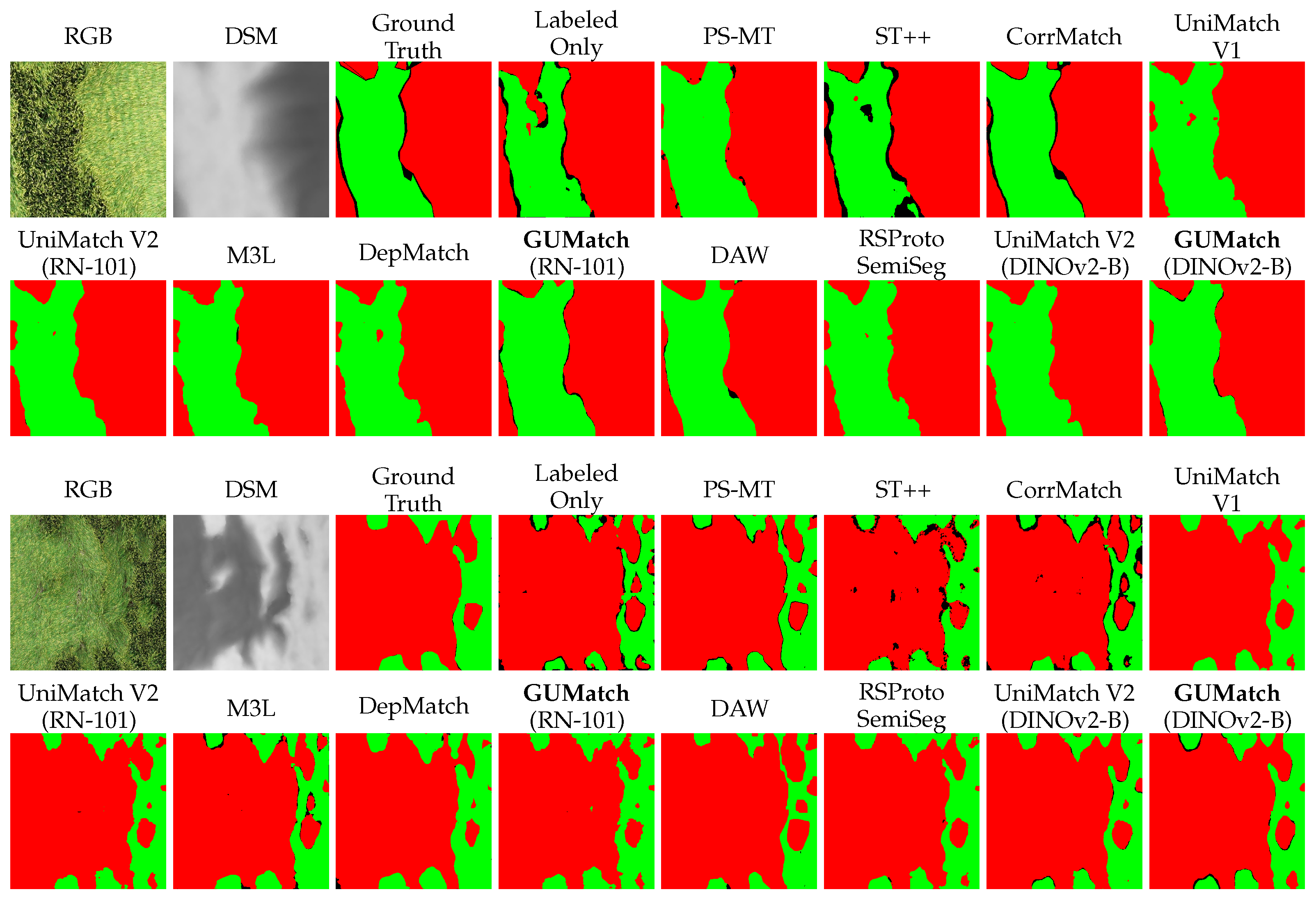
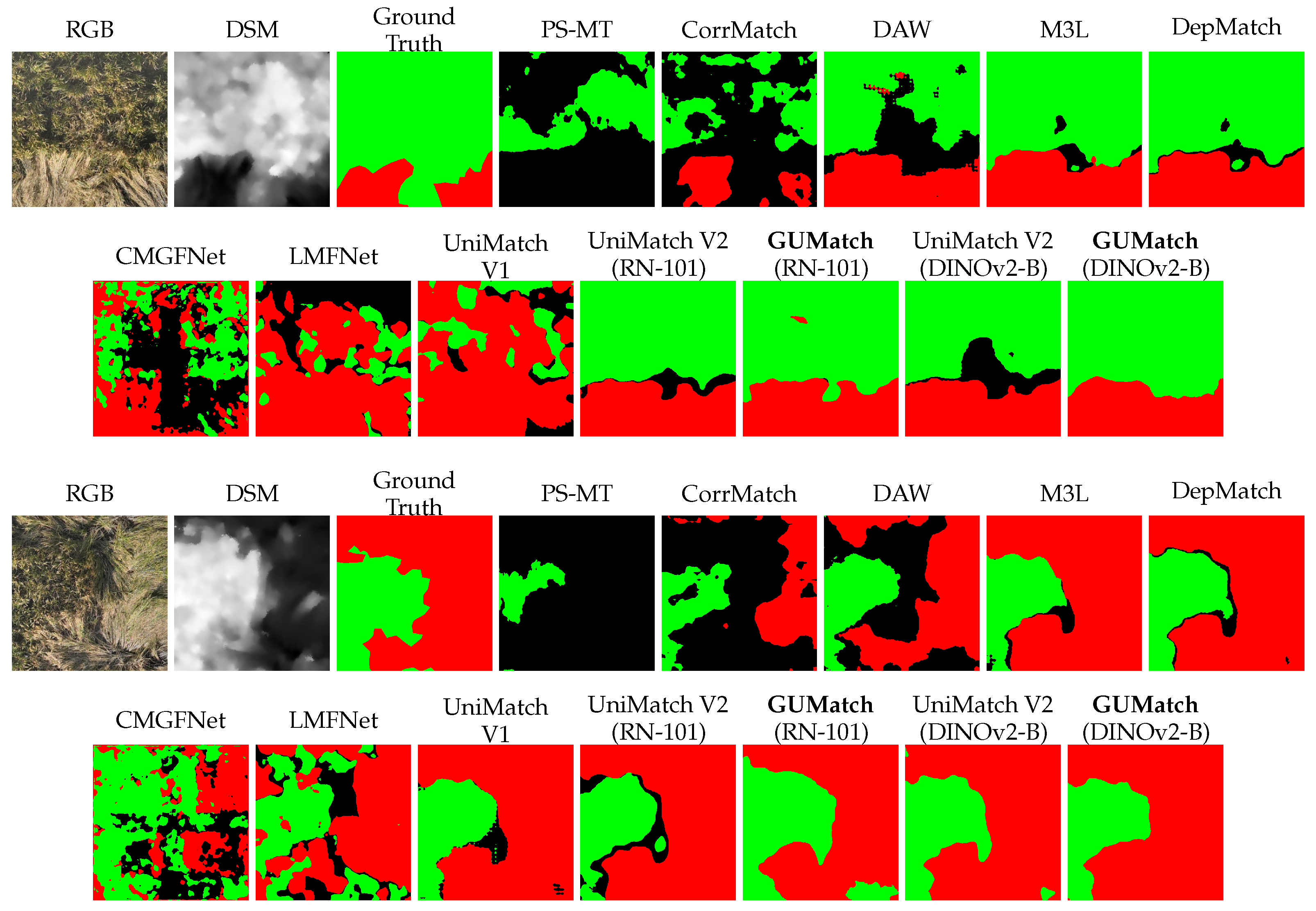
Figure 5 provides local zoom-in comparisons on two representative difficult regions containing mixed crop–background boundaries, fragmented lodged-rice areas, and confusing background patterns. M3L and DepMatch reduce some errors compared with weaker baselines, but still show local fragmentation or boundary discontinuities. GUMatch recovers more complete lodged-rice areas, suppresses background false positives, and preserves clearer local boundaries. The DINOv2-B version is visually closest to the ground truth in both examples.

4.4. Source-Parcel Generalization from HA-P2 to WX-P3

To evaluate cross-region transfer, we conducted an external source-parcel generalization experiment on WX-P3. All models were trained and selected under the 40% labeled setting using only HA-P2. The WX-P3 parcel was then used only for direct testing, with no tile used for parameter updates, model selection, or hyperparameter tuning.

Table 5. Source-parcelgeneralization results on the external WX-P3 set under the 40% labeled setting. Models were trained and selected using only HA-P2; WX-P3 was reserved for direct testing.

Method	Class-Wise IoU (%)			Mean Metrics (%)
	Lodged	Healthy	Background	mIoU	Precision	Recall	F1-Score	PA
PS-MT	31.42	25.64	11.95	23.01	38.93	36.40	36.66	38.78
CorrMatch	65.01	10.40	31.35	35.59	70.28	58.65	48.46	54.73
CMGFNet	67.59	8.47	35.27	37.11	72.16	58.94	49.47	59.58
LMFNet	80.23	29.37	49.84	53.15	76.29	73.25	66.99	72.71
M3L	82.76	28.55	55.60	55.64	78.82	72.80	68.82	76.88
DAW	80.11	38.10	55.20	57.80	76.43	76.20	71.76	75.79
DepMatch	82.54	38.99	59.76	60.43	78.22	75.73	73.78	79.33
UniMatch V2 (RN-101)	79.75	42.30	61.10	61.05	79.16	78.49	74.68	78.06
GUMatch (RN-101)	79.64	48.46	69.40	65.83	82.63	77.59	78.63	82.00
UniMatch V2 (DINOv2-B)	80.44	43.92	64.49	62.95	81.01	77.68	75.82	81.06
GUMatch (DINOv2-B)	79.86	50.34	74.81	68.34	83.36	81.11	80.69	81.79

reports the results.

A clear cross-region domain gap exists. With DINOv2-B, GUMatch drops from 86.72% mIoU on HA-P1 to 68.34% mIoU on WX-P3, confirming that the Wuxi scene is substantially more challenging. Nevertheless, GUMatch remains the strongest method on WX-P3, improving over UniMatch V2 with the same backbone by 5.39 mIoU points. The class-wise results indicate that geometry-guided prompting and pseudo-label calibration help suppress background-driven errors under distribution shift, though lodged-rice IoU is not the highest among all methods.

Figure 6 provides a visual companion: several baselines produce fragmented masks or large background-confusion regions, while GUMatch gives more spatially coherent predictions.

4.5. Ablation Studies

Unless otherwise stated, all ablation experiments use the 20% labeled split with DINOv2-B. We focus on the three main components of GUMatch: AGP for geometry-guided feature prompting, GPL for pseudo-label calibration, and BGR for boundary refinement. We also evaluate the edge-prior extraction and response-normalization functions.

4.5.1. Contribution of the Core Design Elements

Table 6. Ablation of the core design elements on the 20% split.

Setting	AGP	GPL	BGR	mIoU	mF1	BF1
UniMatch V2				82.54	90.12	71.86
+ Fixed Decoder Fusion				83.21	90.63	73.18
+ AGP	Y			83.86	91.05	74.24
+ GPL	Y	Y		84.29	91.31	75.37
GUMatch	Y	Y	Y	84.95	91.69	77.21

shows the progression from a simple RGB–DSM extension to the full geometry-guided design. Fixed decoder summation of DSM features gives only a modest improvement, suggesting that simple multimodal stacking is insufficient. AGP improves the result through reliability gating, GPL further enhances pseudo-label reliability, and BGR gives the best BF1 and mIoU.

4.5.2. Fusion Strategy and Injection Position

We introduce DSM as an adaptive geometric prompt after RGB complementary dropout and before DPT decoding.

Table 7. Ablation of fusion strategy and DSM injection position on the 20% split.

Fusion Strategy	Injection Stage	mIoU (%)	BF1 (%)
Early concatenation	input level	82.89	72.44
Backbone fusion	encoder stage 3–4	82.97	72.87
Fixed addition	before RGB comp-drop	82.94	72.96
Fixed addition	after RGB comp-drop	83.21	73.18
AGP (ours)	after RGB comp-drop	84.95	77.21

supports this choice. Early concatenation and backbone fusion are weaker than decoder-side integration. Injecting DSM after RGB complementary dropout outperforms injection before dropout.

4.5.3. Teacher–Student Modality Configuration

Table 8. Effect of teacher–student modality configuration on the 20% split.

Teacher Input	Student Input	Pseudo-Label Precision (%)	mIoU (%)
RGB	RGB	85.7	82.54
RGB–DSM	RGB	87.4	83.32
RGB	RGB–DSM	85.7	83.57
RGB–DSM	RGB–DSM	88.5	84.95

shows the best performance when both teacher and student receive RGB–DSM inputs. This symmetric setting allows geometry to contribute to both pseudo-label generation and student learning.

4.5.4. Pseudo-Label Quality Analysis

We evaluate pseudo-label quality on the unlabeled training set using hidden annotations only for post hoc evaluation.

Table 9. Pseudo-label quality analysis. Hidden annotations are used only for analysis and never for optimization.

Pseudo-Label Selection	Precision (%)	Recall (%)	Retained Ratio (%)	BF1 (%)
UniMatch V2 (RGB) + raw confidence	85.7	74.4	64.8	68.1
UniMatch V2 + DSM (decoder add) + raw confidence	86.5	75.0	64.3	69.4
GUMatch teacher + raw confidence	87.6	76.1	63.8	70.9
GUMatch teacher + calibrated confidence (full GPL)	88.5	76.8	60.5	72.6

shows that geometry-calibrated confidence retains slightly fewer pixels than raw semantic confidence from the same teacher, but improves precision, recall, and BF1.

4.5.5. Edge-Prior Extraction and Normalization

The DSM edge prior is shared by AGP, GPL, and BGR. We conduct two controlled ablations: fixing normalization and varying edge extraction, and fixing edge extraction and varying normalization.

Table 10. Ablation of DSM edge extraction and response normalization on the 20% DINOv2-B split.

Design Factor	Variant	mIoU (%)	mF1 (%)	BF1 (%)
Edge extraction with fixed mean-exponential normalization
Edge extraction	Sobel, no smoothing	84.31	91.28	75.82
	Gaussian + Scharr	84.87	91.63	76.94
	LoG response	84.05	91.14	75.08
	Canny	83.91	91.02	74.62
	Gaussian + Sobel (ours)	84.95	91.69	77.21
Normalization with fixed Gaussian + Sobel edge extraction
Normalization	Max/min–max	84.18	91.18	75.34
	Percentile clipping	84.62	91.47	76.43
	Mean-linear clipping	84.70	91.53	76.56
	Z-score + sigmoid	84.34	91.30	75.91
	Mean-exp (ours)	84.95	91.69	77.21

shows that Gaussian-smoothed Sobel gives the best overall result. Removing smoothing weakens both mIoU and BF1. Scharr yields close results but offers no clear advantage. LoG and Canny perform worse, especially in BF1. The normalization results support the proposed mean-exponential form, which preserves relative edge strength while smoothly saturating large outliers.

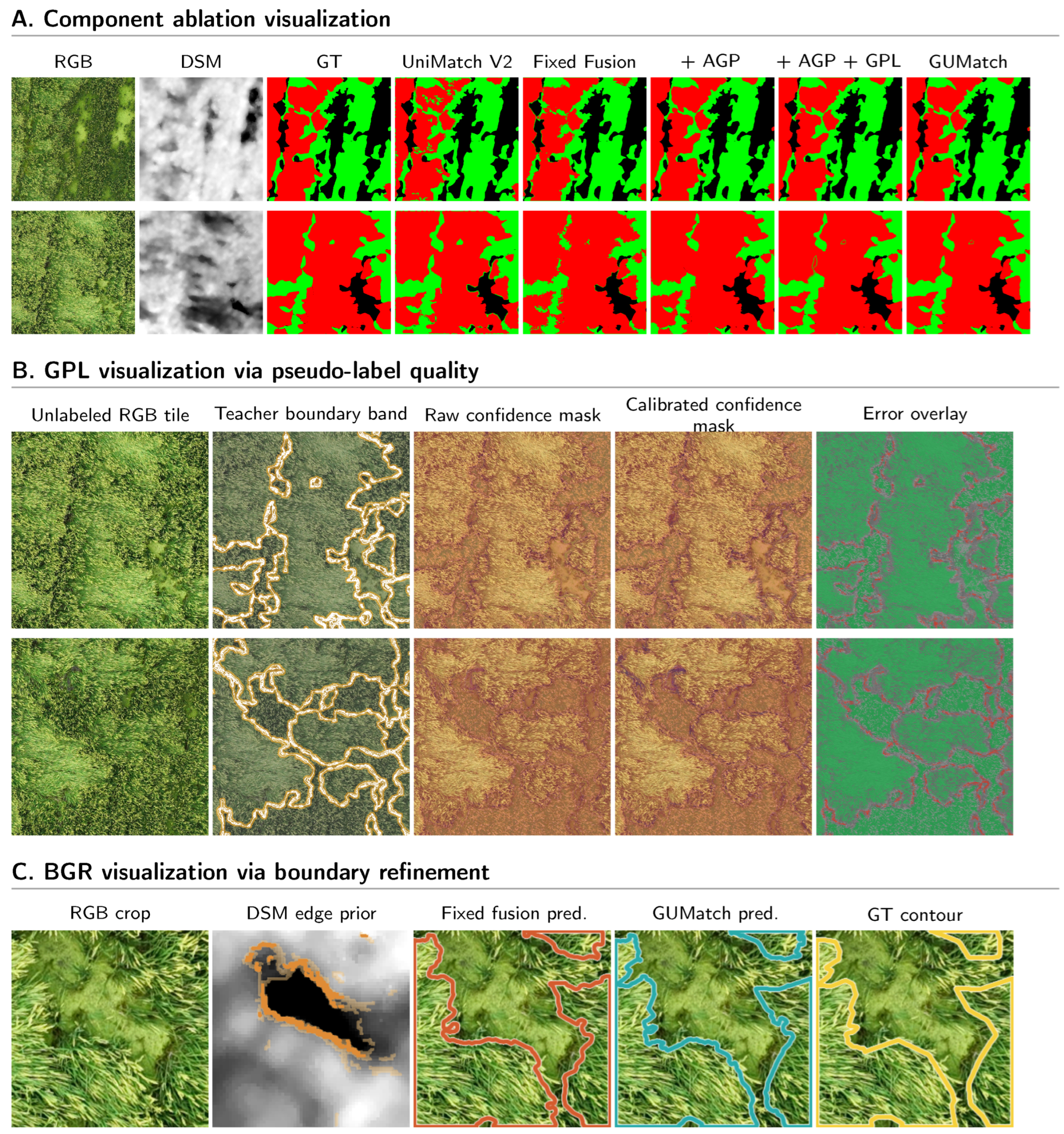
Figure 7 provides mechanism-oriented qualitative analysis. Panel A shows progressive improvement from UniMatch V2 to the full model. Panel B visualizes GPL’s effect on pseudo-label quality. Panel C demonstrates BGR’s boundary refinement.

4.6. Robustness, Sensitivity, and Efficiency Analysis

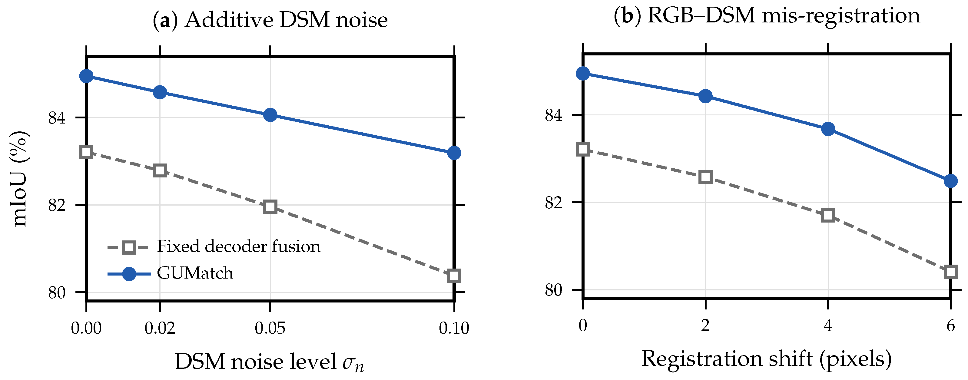
Remote-sensing DSMs may contain spatially correlated reconstruction failures. We therefore focus on structured DSM degradation that better reflects photogrammetric failure patterns, with simpler controlled perturbations reported in Appendix B. Unless otherwise stated, this analysis uses the 20% labeled split with DINOv2-B and compares GUMatch with DepMatch.

4.6.1. Structured DSM Degradation Protocol

We evaluate three structured degradation modes: (1) spatially correlated height distortion, (2) regional topological collapse, and (3) interpolated voids and smoothed holes. Their physical interpretations and severity-specific parameter settings are summarized in

Table 11. Structured DSM degradation settings for robustness evaluation.

Degradation Mode	Physical Interpretation	Mild	Moderate	Severe
Low-frequency height distortion	Correlated canopy/reconstruction drift	β = 0.03,	β = 0.06,	β = 0.10,
		σl = 32 px	σl = 32 px	σl = 32 px
Regional topological collapse	Continuous local surface collapse	area = 10%,	area = 20%,	area = 30%,
		γ = 0.05	γ = 0.75	γ = 1.00
Interpolated voids and smoothed holes	Filled holes and interpolation artifacts	area = 10%,	area = 20%,	area = 30%,
		σh = 16 px	σh = 24 px	σh = 32 px

. Degradation is applied to unlabeled DSMs during semi-supervised training; labeled samples, validation, and test sets remain clean.

Table 12. Results under structured degradation of unlabeled training DSMs on the 20% DINOv2-B split. $\Delta$mIoU = clean-DSM mIoU minus degraded-DSM mIoU.

Training DSM Setting	Level	DepMatch [38]			GUMatch
		mIoU	BF1	$\Delta$mIoU	mIoU	BF1	$\Delta$mIoU
Clean DSM	–	81.49	73.18	0.00	84.95	77.21	0.00
Low-frequency height distortion	Mild	80.68	72.54	0.81	84.57	76.78	0.38
Low-frequency height distortion	Moderate	80.03	71.38	1.46	84.13	76.15	0.82
Low-frequency height distortion	Severe	79.72	69.96	1.77	83.39	75.02	1.56
Regional topological collapse	Mild	80.31	72.04	1.18	84.37	76.50	0.58
Regional topological collapse	Moderate	79.93	70.03	1.56	83.52	75.21	1.43
Regional topological collapse	Severe	78.74	67.21	2.75	82.57	73.72	2.38
Interpolated voids and smoothed holes	Mild	80.77	72.22	0.72	84.55	76.70	0.40
Interpolated voids and smoothed holes	Moderate	80.36	70.58	1.13	83.86	75.74	1.09
Interpolated voids and smoothed holes	Severe	78.68	68.61	2.81	82.61	74.02	2.34

shows that GUMatch maintains higher absolute mIoU and BF1 than DepMatch under all settings, with smaller $\Delta$mIoU values. Regional topological collapse remains the most challenging degradation.

4.6.2. Hyperparameter Sensitivity

We sweep the four most influential parameters around their defaults.

Table 13. Sensitivity analysis on the 20% DINOv2-B split.

Parameter	Default	Low	Mid	High	Range (mIoU)
$\alpha$ (calibration strength)	0.40	0.20	0.60	0.80	84.62–84.95
${\tau }_c$ (pseudo-label threshold)	0.85	0.75	0.80	0.90	84.51–84.95
${\tau }_d$ (DSM-edge threshold)	0.20	0.10	0.30	0.40	84.43–84.95
${\lambda }_e$ (BGR weight)	0.5	0.1	1.0	2.0	84.30–84.95

shows that mIoU varies by less than 0.7 points across the swept ranges, and GUMatch’s superiority over the strongest non-GUMatch baseline is preserved.

We additionally evaluated three boundary objectives within BGR.

Table 14. Ablation of the boundary objective inside BGR on the 20% DINOv2-B split.

Boundary Loss for BGR	mIoU (%)	BF1 (%)
Dice on binarized maps	84.51	76.18
Active-contour-style [32]	84.62	76.41
L1 amplitude (ours)	84.95	77.21

shows that the L1 formulation yields the best BF1.

4.6.3. Computational Cost

Table 15. Efficiency comparison on the 20% split.

Method	Params (M)	FLOPs (G)	FPS	mIoU (%)
UniMatch V2	62.8	164.2	18.7	82.54
Fixed decoder fusion	68.1	171.4	17.9	83.21
GUMatch	69.0	173.8	17.4	84.95

shows that DINOv2-B GUMatch adds only moderate parameters and FLOPs compared with UniMatch V2, with the extra cost mainly from the lightweight DSM encoder and adaptive prompting layers.

5. Conclusions

This study proposes GUMatch, a geometry-guided semi-supervised framework that leverages UAV RGB–DSM data for rice-lodging segmentation with limited annotations. By selectively using DSM-derived height and boundary cues, GUMatch suppresses unreliable geometric evidence while preserving RGB appearance as the primary semantic source. Experiments on the HA-P2→HA-P1 benchmark demonstrate consistent mIoU improvements across 10% to 40% labeled ratios with both RN-101 and DINOv2-B backbones, reaching up to 86.72% mIoU. External testing on WX-P3 confirms a substantial domain gap but also shows that GUMatch maintains stronger cross-region performance than the corresponding UniMatch V2 baseline. Together, these results demonstrate that reliability-aware geometric guidance enhances annotation-efficient lodging mapping when RGB appearance is ambiguous. Future work will extend validation across broader agricultural conditions and sensing settings, while exploring lightweight deployment, improved robustness to degraded or missing modalities, and applications to other structure-sensitive remote-sensing tasks.