Article

Boot-Shaped Terrain Screening and Deep Learning Semantic Segmentation for Landslide-Hazard Candidate Extraction from Airborne LiDAR DEM: A Case Study in Zhenxiong County, China

1
School of Transportation Science and Engineering, Beihang University, Beijing 100191, China
2
China Institute of Geo-Environment Monitoring (Guide Center of Prevention Technology for Geo-Hazards, MNR), Beijing 100081, China
*
Author to whom correspondence should be addressed.
Remote Sens. 2026, 18(17), 2983; https://doi.org/10.3390/rs18172983
Submission received: 15 July 2026 / Revised: 27 August 2026 / Accepted: 31 August 2026 / Published: 3 September 2026

Highlights

What are the main findings?
  • A parameterized boot-shaped terrain screening rule formalizes the steep-upper–gentle-lower terrain morphology, while sensitivity analysis shows that the resulting rule-derived candidate definition is materially dependent on the screening parameters.
  • DeepLabV3+ achieved the highest mean model–rule agreement among the evaluated architectures, while DEM + slope was retained as a parsimonious two-channel input and the contribution of aspect was configuration-dependent.
What are the implications of the main findings?
  • Expert-informed geomorphological rules can provide structured supervision for learning terrain-screening patterns when independently verified inventories are limited, although the resulting predictions should be interpreted as rule-derived candidates rather than confirmed landslide hazards.
  • Once trained, the segmentation surrogate operates directly on DEM and slope-gradient rasters without reconstructing slope units and longitudinal profiles for each inference run, thereby simplifying the operational candidate-screening workflow.

Abstract

Automated screening of geomorphologically defined landslide potential-hazard candidates from high-resolution topographic data remains challenging in mountainous regions where comprehensive field inventories are unavailable. This study proposes a two-stage framework for extracting rule-defined boot-shaped terrain candidates from airborne LiDAR digital elevation model (DEM) data. First, an expert-informed screening rule formalizes a steep-upper–gentle-lower terrain morphology using representative longitudinal profiles of slope units, and the screened units are converted into rule-derived reference masks. Second, semantic segmentation models are trained to approximate these reference patterns directly from DEM-derived raster inputs. Four architectures—U-Net, U-Net++, DeepLabV3+, and SegFormer-B0—were evaluated using 406 patches of 256 × 256 pixels at 2 m resolution from four LiDAR-covered subregions in Zhenxiong County, China. Under spatially grouped three-fold cross-validation, DeepLabV3+ with DEM + slope-gradient input and Dice + Focal loss achieved a mean pixel-level F1-score of 0.351, mIoU of 0.557, and Patch-F1 of 0.814. Input-feature experiments showed that slope-gradient information was particularly informative, whereas the incremental contribution of aspect was configuration-dependent; DEM + slope was retained as a parsimonious two-channel input. Sensitivity analysis showed that the rule-derived candidate definition changed materially with the screening parameters. Leave-one-subregion-out evaluation yielded a macro-averaged F1 of 0.321, indicating measurable within-county cross-subregion transfer. However, whole-area evaluation under natural candidate prevalence reduced the macro-average F1 to 0.072 at a fixed threshold and 0.095 using validation-derived operating thresholds. These results indicate that the proposed model is best interpreted as a raster-based surrogate for rule-derived geomorphological screening rather than as an independently validated landslide detector.

1. Introduction

Landslides are major natural hazards that cause substantial loss of life worldwide [1]. Mountainous regions of southwestern China are particularly susceptible to slope instability because of their steep relief, tectonic activity, and strongly dissected terrain [2,3].
The Wumeng Mountainous Region is characterized by deeply dissected mountainous terrain and complex geological conditions. In Zhenxiong County, Wu et al. [4] described the source area of the catastrophic landslide that occurred on 22 January 2024 as exhibiting a “boot-shaped terrain” configuration. This regional observation motivates the terrain concept investigated in the present study. Rather than treating this morphology as a deterministic precursor of slope instability, we abstract it as a steep-upper–gentle-lower longitudinal terrain pattern and formalize it as an operational geomorphological screening criterion.
Zhenxiong County in northeastern Yunnan Province was selected as the study area. The catastrophic landslide of 22 January 2024 in Liangshui Village resulted in severe casualties and highlighted the need for improved screening of landslide-prone terrain [4]. The ability to identify terrain warranting further investigation before slope failure is important for proactive disaster-risk reduction and land-use planning [5].
Conventional approaches to landslide assessment include inventory- and geomorphology-based investigation [6,7] and data-driven susceptibility modelling using conditioning factors such as slope, aspect, lithology, land use, and precipitation [8,9]. Statistical and machine-learning methods, including logistic regression [10], support vector machines [11], and random forests [12], have been widely used for landslide susceptibility mapping, generally producing spatial susceptibility estimates from predefined conditioning variables.
The emergence of deep learning, and semantic segmentation in particular, has opened new possibilities for pixel-level landslide detection and mapping from remote-sensing imagery [13,14]. Architectures such as U-Net [15], DeepLabV3+ [16], and Transformer-based segmentation models [17,18] provide widely used methodological foundations for this task. Chen et al. [19] demonstrated automated landslide detection from multi-temporal remote-sensing imagery in mountainous urban settings, while Ji et al. [20] introduced the open Bijie landslide dataset containing optical imagery, DEM information, and interpreted landslide boundaries. Recent studies have further explored hybrid CNN–Transformer architectures [21], multi-scale feature fusion [22], attention-based segmentation [23], and learning strategies for class-imbalanced landslide mapping [24].
Despite these advances, three limitations remain relevant to the present task. First, many landslide-detection studies rely strongly on optical remote-sensing imagery, whose effectiveness may be reduced by cloud cover, vegetation occlusion, and limited visibility of underlying terrain [18,25]. Second, supervised deep-learning methods depend on reliable labelled inventories, whereas landslide inventories can be incomplete, spatially biased, and inconsistent among mapping sources [6,26]. Third, purely data-driven workflows do not necessarily encode explicit geomorphological constraints, and biases in the spatial distribution or collection of landslide labels can affect both model predictions and their physical interpretation [27]. These considerations motivate the use of topographic data and explicit geomorphological screening in the present study.
Airborne LiDAR-derived DEMs provide a complementary source of information because they describe bare-earth topography beneath vegetation and can reveal terrain morphology that may be difficult to interpret directly from optical imagery [28]. Recent deep-learning studies have increasingly incorporated DEM-derived terrain information into landslide detection. For example, Li et al. [25] proposed the multimodal DemDet framework combining LiDAR-derived terrain information with optical imagery for forested landslide detection, while Liu et al. [29] developed a feature-fusion segmentation network integrating high-resolution remote-sensing imagery with DEM-derived terrain features. Hybrid approaches have also combined satellite imagery with DEM-derived topographic channels [21]. These studies demonstrate the value of topographic information as a complement to spectral imagery, while motivating further investigation of whether DEM-derived terrain variables alone can support approximation of a specifically defined geomorphological screening pattern.
The second limitation, namely the scarcity and inconsistency of labeled landslide data, motivates the use of rule-derived candidate masks as an alternative source of supervision. In many mountainous regions, comprehensive and spatially consistent landslide inventories are difficult to obtain, and available inventories are often biased toward post-event mapping or visually evident surface failures. This limitation is particularly relevant when the research target is not a complete landslide inventory, but a specific terrain morphology that can be described by expert geomorphological knowledge. In this context, geomorphologically interpretable terrain-screening rules provide a practical way to generate candidate labels from DEM-derived topographic information, thereby reducing the dependence on large manually interpreted landslide inventories.
The third limitation, namely the lack of explicit geomorphological priors in many deep learning workflows, motivates the use of slope units as the basic terrain analysis units. Slope units are terrain compartments bounded by ridge and valley lines that represent natural geomorphological units over which gravitational mass movements may initiate and propagate [30,31]. Compared with regular grid cells, slope-unit-based approaches provide physically meaningful boundaries, reduce within-unit topographic heterogeneity, and better capture whole-slope processes [32]. Recent studies have begun to combine slope units with deep learning; for example, Wang et al. [33] applied graph convolutional networks to slope-unit-based susceptibility mapping by treating each slope unit as a node in a geomorphological graph. However, few studies have explicitly used slope-unit-level geomorphological rules to generate rule-derived candidate masks and then trained deep learning models to approximate such rule-based terrain-screening outputs.
This study formalizes the boot-shaped terrain description reported for the Zhenxiong landslide [4] as a quantitative geomorphological screening criterion. The targeted pattern is represented as a steep-upper–gentle-lower transition along a representative longitudinal slope-unit profile. Rather than assuming that this morphology constitutes an independently validated precursor of landslide occurrence, the proposed rule defines a reproducible terrain-candidate class for subsequent analysis. By coupling this explicit screening procedure with semantic segmentation, the framework uses the resulting rule-derived masks as structured supervisory targets and evaluates whether their spatial patterns can be approximated directly from DEM-derived raster inputs. The segmentation model is therefore intended as a raster-based surrogate of the upstream screening procedure rather than as an independently supervised landslide detector.
The specific objectives of this study are as follows:
(1)
To formalize boot-shaped terrain morphology as a parameterized screening criterion based on representative longitudinal profiles of slope units, and to quantify the sensitivity of the resulting rule-derived candidate definition to the screening parameters;
(2)
To compare four representative semantic segmentation architectures (U-Net, U-Net++, DeepLabV3+, and SegFormer-B0) for approximating the rule-derived boot-shaped terrain masks from DEM-derived raster inputs;
(3)
To evaluate the contribution of DEM-derived terrain variables through controlled input-feature comparisons and to identify a parsimonious raster-input configuration for subsequent surrogate-model evaluation;
(4)
To evaluate model–rule agreement under complementary spatial settings, including pixel- and patch-level evaluation on the controlled patch dataset, cross-subregion transfer, and whole-area evaluation under the natural prevalence of rule-derived candidates.
The remainder of this paper is organized as follows. Section 2 describes the study area and the LiDAR DEM data. Section 3 presents the methodology, including the boot-shaped terrain screening procedure, dataset construction, and deep learning segmentation architecture. Section 4 presents the qualitative and quantitative results, including architecture, input-feature, and loss-function comparisons, sensitivity analysis of the rule-derived candidate definition, cross-subregion transfer, and whole-area natural-prevalence evaluation. Section 5 discusses the findings, limitations, and future research directions. Section 6 summarizes the main conclusions.

2. Materials and Methods

2.1. Study Area

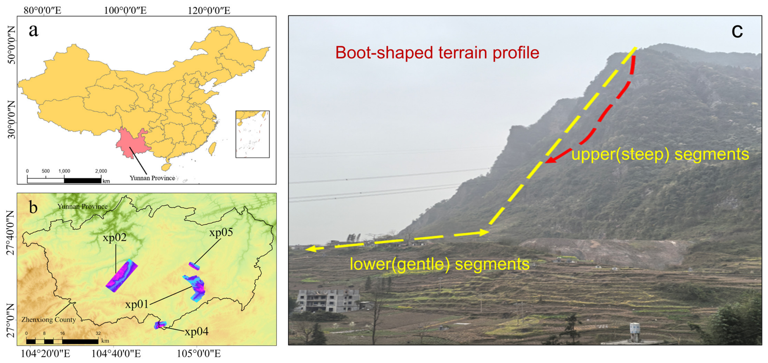
The study area is located in Zhenxiong County, northeastern Yunnan Province, China (Figure 1a,b), approximately between 27°17′–27°50′N and 104°18′–105°19′E. Zhenxiong County covers approximately 3696 km2 and is characterized by strongly dissected mountainous terrain and substantial topographic relief [34]. The four LiDAR-covered subregions investigated in this study span elevations from approximately 989 to 2324 m according to the valid raster coverage summarized in Table 1.
Zhenxiong County has a complex geological setting characterized by folded and faulted strata and pronounced terrain dissection [34]. At the site of the catastrophic Liangshui landslide of 22 January 2024, Wu et al. [4] reported a steep slope with a height difference of approximately 250 m and described the source-area terrain as “boot-shaped”; the local lithology consists predominantly of siltstone and mudstone of the Triassic Feixianguan Formation. These observations provide regional geomorphological context for the boot-shaped screening concept investigated in this study, but the morphology is not assumed here to constitute a deterministic indicator of slope instability.
Landslides are widespread in Zhenxiong County. A recent county-scale inventory identified 3979 landslide relics covering approximately 319.20 km2, with higher landslide concentrations associated with dissected mountainous terrain and well-developed drainage systems [34]. Seasonal precipitation is concentrated during the summer rainy season and constitutes an important regional triggering background, although precipitation is not used as an input variable in the present screening or segmentation framework [34].
Four subregions within Zhenxiong County were selected for this study based on the availability of high-resolution airborne LiDAR coverage: xp01, xp02, xp04, and xp05 (Figure 1b). Based on the valid raster coverage used in the subsequent analyses, the effective LiDAR-covered areas of the four subregions were approximately 53.32 km2, 73.29 km2, 12.00 km2, and 8.62 km2, respectively, yielding a total valid coverage of approximately 147.23 km2. These subregions encompass the range of elevations and surface-gradient conditions represented in the available LiDAR dataset.

2.2. LiDAR DEM Data

The primary data source was an airborne LiDAR-derived digital elevation model (DEM) with a spatial resolution of 2 m covering the four study subregions. According to the acquisition and processing metadata provided by the data provider, the LiDAR point clouds were acquired by an authorized surveying agency using a fixed-wing aircraft equipped with a RIEGL VQ-1560ii airborne laser scanning system (RIEGL Laser Measurement Systems GmbH, Horn, Austria) at an approximate flight altitude of 1200 m, with an average point density of approximately 12 points m−2. The point clouds underwent noise filtering, ground-point classification, interpolation, and coordinate transformation before generation of the final 2 m DEM product. The DEM was provided in the CGCS2000/3-degree Gauss–Kruger CM 105E projected coordinate reference system (EPSG:4544).
A spatially continuous slope-gradient raster was derived from the 2 m DEM using a Horn-style 3 × 3 weighted finite-difference operator and expressed in degrees from 0° to 90°. This raster represents local terrain steepness at the raster-cell scale and was evaluated as a candidate input variable for semantic segmentation. It is distinct from the profile-segment inclination angles used in the Stage-1 geomorphological screening rule, which were calculated only along the representative longitudinal profiles of individual slope units.
Terrain aspect was derived from the same DEM gradient information and represented jointly by its sine and cosine components to avoid the circular discontinuity at 0°/360°. Both components were retained together whenever aspect was included in an input configuration. The controlled evaluation of DEM, slope gradient, and aspect as candidate model inputs is described in Section 3.2.3, with the corresponding results presented in Section 4.3.
The DEM, slope-gradient, sine-aspect, and cosine-aspect rasters were co-registered on the same 2 m grid in each subregion. Table 1 summarizes the spatial dimensions, valid LiDAR-covered area, elevation range, slope-gradient range, and proportion of valid DEM pixels for the four study subregions.

3. Methodology

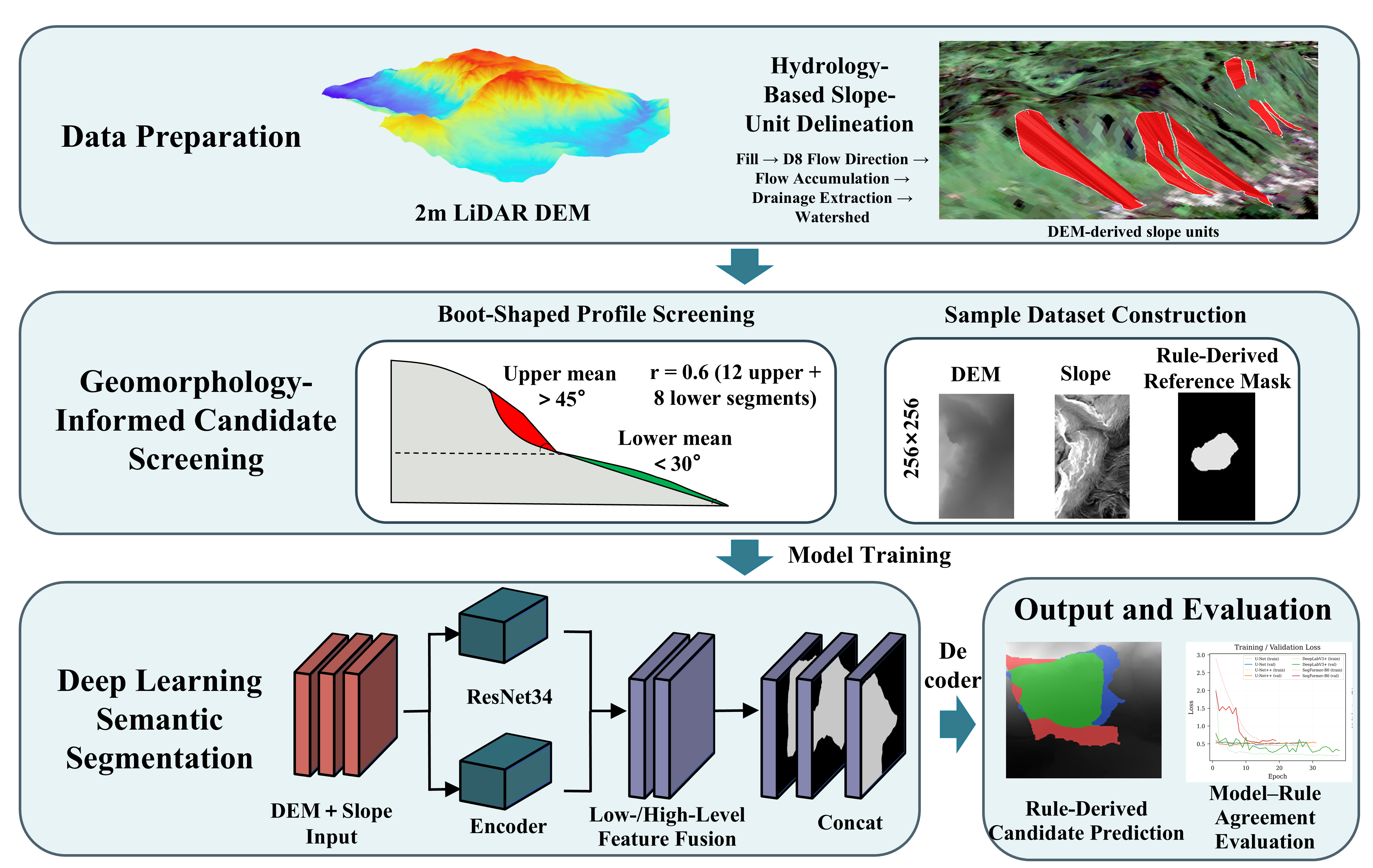
The proposed framework consists of two sequential stages (Figure 2).
In Stage 1, a rule-based geomorphological screening procedure identifies slope units exhibiting the prescribed steep-upper–gentle-lower longitudinal morphology and converts the retained candidates into rule-derived reference masks. In Stage 2, semantic segmentation models are trained on DEM-derived raster patches to approximate these reference patterns. The selected segmentation surrogate subsequently operates directly on co-registered DEM and slope-gradient rasters and produces reference-positive probability maps without reconstructing slope units or longitudinal profiles during inference. Thus, explicit geomorphological knowledge enters the learning process through the rule-derived supervisory targets, while final deployment is performed directly in raster space.

3.1. Boot-Shaped Terrain Screening

The boot-shaped terrain concept used in this study is motivated by regional engineering-geological observations in Zhenxiong County, including the steep-upper–gentle-lower terrain description reported for the 2024 Liangshui landslide [4]. In this study, this morphology is abstracted as a longitudinal geometric pattern for terrain screening rather than as a deterministic indicator of slope instability. The targeted form is illustrated in the annotated field photograph in Figure 1c.
In this study, the observed morphology is formalized as a geomorphological screening criterion rather than as a deterministic indicator of landslide occurrence. The purpose of the rule-based stage is therefore to identify slope units exhibiting the specified boot-shaped longitudinal geometry and to generate terrain-candidate masks for subsequent deep learning experiments. These rule-derived candidates represent terrain units warranting further interpretation rather than independently verified landslide sites.

3.1.1. Slope Unit Delineation and Profile Extraction

The terrain surface was partitioned into slope units, defined as geomorphologically meaningful terrain compartments bounded primarily by ridge and drainage lines [30,31]. Compared with regular raster cells, slope units provide spatial entities that better preserve whole-slope topographic organization and are therefore widely used as basic analysis units in landslide susceptibility and terrain-based hazard assessment [32].
Slope units were delineated in ArcGIS Pro 3.4.2 using a hydrology-based workflow applied to the 2 m DEM. The DEM was first processed by sink filling, followed by D8 flow-direction and flow-accumulation calculations. The D8 algorithm was used only at this hydrology-based slope-unit delineation stage to support drainage extraction and watershed-based terrain subdivision; it was not used to trace the representative longitudinal profiles described below. Drainage lines were subsequently extracted from the flow-accumulation raster, and ridge and drainage boundaries were used to derive individual slope units. During workflow development, flow-accumulation thresholds of 500, 1000, and 2000 cells were examined. A threshold of approximately 1000 cells was retained by jointly considering the resulting slope-unit size, correspondence between the extracted boundaries and the observed terrain morphology, and the overall number of slope units. Following automated delineation, a limited number of slope-unit boundaries were manually refined with reference to local terrain morphology and available remote-sensing imagery. The imagery was used only for boundary quality control and was not used as an input to the subsequent deep-learning segmentation model or as an additional criterion in the boot-shaped profile rule.
After slope-unit delineation, one representative longitudinal profile was constructed for each slope unit using a custom Python geometric procedure. The highest- and lowest-elevation vertices of the slope-unit boundary were first identified and connected to define a longitudinal baseline. The baseline was divided into 20 equal intervals. At each internal division position, a cross-slope line approximately perpendicular to the baseline was constructed and intersected with the two sides of the slope-unit boundary. The midpoint between the two boundary intersections was then retained as an intermediate profile vertex. The representative longitudinal profile was formed by connecting the highest-elevation endpoint, the successive cross-slope midpoints, and the lowest-elevation endpoint. This construction provides a centrally located and consistently defined longitudinal representation of each slope unit, while avoiding reliance on a D8 flow path for profile extraction.
For the valid profiles retained for subsequent analysis, the 21 ordered profile vertices defined 20 consecutive longitudinal segments. The inclination angle of each segment was calculated directly from the horizontal distance and elevation difference between two adjacent profile vertices, rather than as the mean value of an underlying slope raster. Specifically, for adjacent vertices ( x i , y i , z i ) and ( x i + 1 , y i + 1 , z i + 1 ), the segment inclination was calculated as the arctangent of the absolute elevation difference divided by the corresponding horizontal distance and expressed in degrees. The resulting 20-element vector ( α 1 , α 2 , …, α N ) was subsequently used to quantify the contrast between the upper and lower portions of the profile in Section 3.1.2.
The 20-segment representation was adopted as a study-specific compromise between longitudinal terrain detail and consistent comparison among slope units. The mean profile length in the investigated dataset was approximately 348 m. A substantially coarser subdivision, such as 10 segments, was considered insufficient for resolving the targeted longitudinal slope-form variation, whereas excessive subdivision would reduce the spatial support of individual segments, particularly for shorter profiles relative to the 2 m DEM resolution. Twenty segments were therefore retained as a common representation suitable for the majority of slope units in the study area. Across the four study subregions, 18,601 slope units were delineated before application of the boot-shaped screening criteria. These profile-segment inclination angles were used exclusively for the Stage-1 geomorphological screening rule and are distinct from the spatially continuous slope-gradient raster used as a deep-learning input channel in Section 3.2.3.

3.1.2. Boot-Shaped Profile Criteria

The boot-shaped screening rule quantifies the steep-upper–gentle-lower contrast along each 20-segment representative longitudinal profile. Let the segment-inclination vector of a slope unit be denoted by ( α 1 ,   α 2 , …, α N ), where N = 20 and αi is the inclination angle, in degrees, of the i-th consecutive profile segment calculated from the elevation difference and horizontal distance between its two adjacent profile vertices. The segments are ordered from the upper to the lower part of the slope. A partition fraction r is used to divide the profile into an upper and a lower portion, with the partition index defined as k = r × N . The mean inclination angles of the upper and lower portions are then calculated as:
α ¯ u p p e r = 1 k × i = 1 k α i
α ¯ l o w e r = 1 20 k × k + 1 20 α i
The rule-derived boot-shaped terrain indicator is then defined as:
C b o o t = 1 , α ¯ u p p e r > θ u p p e r   a n d   α ¯ l o w e r < θ l o w e r   , 0 , o t h e r w i s e   ,
where θ u p p e r and θ l o w e r denote the threshold values applied to the mean upper- and lower-profile segment inclinations, respectively. A slope unit satisfying both inequalities is retained as a rule-derived boot-shaped terrain candidate. This classification indicates conformity with the prescribed geomorphological screening rule and should not be interpreted as confirmation of landslide occurrence or instability.
The predefined reference configuration used for candidate generation in the main experiments was θ u p p e r = 45°, θ l o w e r = 30°, and r = 0.6. With N = 20, this setting assigns the first 12 segments to the upper portion and the remaining 8 segments to the lower portion of the profile. These values operationalize the regional expert-informed concept of a distinctly steep upper slope transitioning into a gentler lower slope and were used as the reference configuration throughout the main model experiments. They are not assumed to represent universally optimal or physically unique thresholds. Their influence on candidate abundance, spatial extent, and subsequent model–rule agreement is explicitly evaluated through the parameter-sensitivity analysis described in Section 4.5.
To examine the sensitivity of the rule-derived candidate definition to the three profile parameters, nine predefined parameter combinations were evaluated: (40°, 30°, 0.6), (45°, 30°, 0.6), (50°, 30°, 0.6), (45°, 25°, 0.6), (45°, 35°, 0.6), (45°, 30°, 0.5), (45°, 30°, 0.7), (40°, 25°, 0.5), and (50°, 35°, 0.7), where each tuple denotes ( θ u p p e r , θ l o w e r , r). The configuration (45°, 30°, 0.6) was treated as the reference setting. For each parameter combination, the rule-based screening procedure was rerun to generate a corresponding candidate set and rule-derived reference masks, after which the patch dataset and spatial folds were reconstructed using the same procedures described in Section 3.2.2 and Section 3.3.3. DeepLabV3+ with DEM + slope input and Dice + Focal loss was then evaluated across the three spatial folds using a fixed random seed, so that differences among parameter settings could be examined under a consistent model configuration.
Sensitivity was assessed from two complementary perspectives. First, changes in the rule-derived candidate sets were quantified relative to the reference configuration using candidate abundance and spatial-overlap measures, including Jaccard overlap, Dice overlap, retention of reference-configuration candidate pixels, relative candidate area, and symmetric-difference area. Second, the corresponding segmentation performance was evaluated using the model–rule agreement metrics defined in Section 3.3.4. These analyses were used to characterize how the screening parameters affect candidate definition and downstream learnability; they were not used to establish the physical correctness or optimality of any parameter setting for real landslides.

3.1.3. Geometric Filtering of Candidate Slope Units

Slope units satisfying the boot-shaped profile criterion were further screened using area and shape constraints before raster-mask generation. Candidate units with an area smaller than 3000 m2 or larger than 500,000 m2 were excluded. At the 2 m DEM resolution, the lower-area threshold corresponds to approximately 750 raster pixels. In addition, the shape of each candidate slope unit was characterized using the aspect ratio of its minimum bounding rectangle, defined as the ratio of the longer side to the shorter side. Units with an aspect ratio greater than 12 were excluded to reduce the inclusion of exceptionally elongated terrain partitions that are less compatible with the slope-unit geometry targeted in this study.
These thresholds were implemented as operational geometric constraints for constructing the rule-derived candidate set rather than as universal physical criteria for landslide occurrence or instability. After application of the profile-based screening and geometric filtering procedures, 192 candidate slope units were retained across the four study subregions, including 64 in xp01, 100 in xp02, 20 in xp04, and 8 in xp05. These retained units were subsequently rasterized and post-processed to generate the rule-derived reference masks described in Section 3.2.1.

3.2. Dataset Construction

3.2.1. Rule-Derived Reference Mask Generation

The reference masks used for model training and evaluation were derived from the boot-shaped terrain screening procedure described in Section 3.1 rather than from an independently verified landslide inventory. Specifically, slope units satisfying the profile-based criterion and subsequent geometric constraints were treated as rule-derived terrain candidates. As described in Section 3.1.1, the initial slope units were generated from the DEM using a hydrology-based workflow, with limited manual refinement of selected boundaries using terrain morphology and available remote-sensing imagery for quality control. This ancillary imagery was not used to define the boot-shaped profile criterion, to assign candidate status independently of the rule, or as an input to the semantic segmentation models. These candidates therefore encode conformity with the prescribed geomorphological screening procedure and do not constitute confirmed landslide occurrences or independently validated hazard boundaries. Throughout the remainder of this study, the resulting binary masks are referred to as rule-derived reference masks, or simply reference masks for brevity.
Accordingly, the semantic segmentation models were trained to approximate the spatial pattern represented by these reference masks from DEM-derived raster inputs. The reported segmentation metrics therefore quantify model–rule agreement rather than accuracy against independently verified landslide ground truth.
Each retained candidate slope-unit polygon was rasterized independently onto the 2 m DEM grid using the rasterio.features.rasterize function [35]. Independent rasterization was used to preserve the spatial identity of individual candidate units before their binary masks were combined on the common raster grid. A fixed morphological post-processing sequence was then applied to the rasterized candidate masks: (1) a 5 × 5 binary closing operation to fill small gaps and discontinuities; (2) a 3 × 3 binary opening operation to suppress small isolated features and narrow protrusions; (3) filling of enclosed holes; and (4) removal of connected components smaller than 200 pixels, corresponding to approximately 800 m2 at the 2 m raster resolution.
These morphological settings were implemented as fixed raster post-processing parameters to regularize the rule-derived masks before patch extraction. They were not optimized against an independent landslide inventory and should therefore be interpreted as operational mask-processing settings rather than physically calibrated landslide-boundary parameters. The post-processed binary masks, rather than the original vector polygons, were used as the pixel-level reference targets for all subsequent patch extraction, model training, and evaluation.

3.2.2. Patch Sampling Strategy

Raster patches of 256 × 256 pixels were extracted from the DEM and the corresponding co-registered terrain-derivative layers. At the 2 m spatial resolution, each patch covers an approximately 512 m × 512 m ground area. Positive patches were sampled around the retained rule-derived candidate slope units, with the candidate-unit centroid used as the primary patch center. For candidate units with an area greater than 15,000 m2, one additional spatially offset patch was generated to increase spatial coverage of the candidate within the patch dataset. A patch was retained as positive only when it contained at least 100 reference-positive pixels (approximately 400 m2 at 2 m resolution), thereby excluding nearly empty patches produced by clipping or edge effects. This threshold was an operational patch-inclusion criterion rather than a minimum physical size criterion for a landslide or potential hazard. The 15,000 m2 criterion was likewise used only as a sampling rule for increasing patch coverage of comparatively large candidate units and was not treated as a geomorphological or landslide-size threshold.
Reference-negative patches were sampled from locations outside the rule-derived candidate masks. Sample locations were required to be at least 300 m from the boundary of any reference-positive candidate unit, reducing the likelihood that candidate morphology was immediately adjacent to the sampled patch center. The 300 m distance was implemented as an operational sampling buffer to reduce immediate adjacency between negative-patch centers and rule-derived candidates; it was not treated as a physically calibrated exclusion distance. Patches containing NoData values in any required raster channel were excluded.
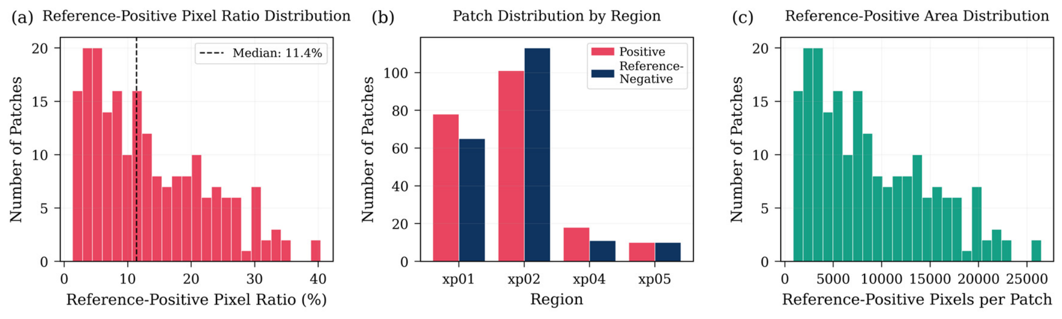
After application of the sampling and raster-validity criteria, the final dataset contained 406 patches, comprising 207 reference-positive patches and 199 reference-negative patches. The resulting positive-to-negative patch ratio was therefore approximately 1:1. The composition of the patch dataset, including the distribution of reference-positive pixel ratios, regional patch counts, and reference-positive pixel counts per positive patch, is summarized in Figure 3. This near-balanced patch composition was designed for controlled model training and comparative evaluation and does not reproduce the natural prevalence of rule-derived candidates across the complete LiDAR-covered regions. Moreover, even within positive patches, reference-positive pixels occupy only a fraction of the patch area, resulting in substantial pixel-level class imbalance. Consequently, patch-level presence/absence metrics are treated as auxiliary measures of controlled screening performance rather than as estimates of operational whole-area performance. A separate whole-area evaluation under the natural candidate prevalence is therefore included in the revised evaluation protocol.

3.2.3. Input Feature Design

Each patch was stored as a multi-channel NumPy array with a spatial size of 256 × 256 pixels, where the number of channels depended on the terrain-variable configuration used in each experiment. The candidate terrain variables consisted of DEM elevation, slope gradient, and terrain aspect represented by its sine and cosine components. The original physical values were retained during patch generation: elevation was stored in meters, slope in degrees, and the two aspect components in the interval [−1, 1]. Per-channel z-score normalization was performed at training time, with the mean and standard deviation calculated exclusively from the training partition of each spatial cross-validation fold and subsequently applied to the corresponding validation and test partitions. This procedure prevented information from the validation or test data from being used in the estimation of normalization statistics.
The slope-gradient raster used as a neural-network input should be distinguished from the profile-segment inclination angles used in the Stage-1 screening rule. The latter are one-dimensional geometric quantities calculated between adjacent vertices of each representative longitudinal profile and are used only to determine whether a slope unit satisfies the boot-shaped criterion. In contrast, the slope-gradient raster is a spatially continuous DEM derivative calculated independently for every raster cell and co-registered with the DEM. It is used only as a terrain input feature for semantic segmentation. Therefore, the deep-learning model does not receive the 20 profile-segment inclination values or the extracted profile lines as input.
Representative examples of the terrain variables and their corresponding rule-derived reference masks are shown in Figure 4. Four raster channels were available for input-feature evaluation: DEM, slope, sin(Aspect), and cos(Aspect). The sine and cosine components jointly represent terrain aspect as a single circular variable rather than as two independent geomorphological features.
For the raster input features, slope gradient and terrain aspect were derived from the DEM using a Horn-style 3 × 3 weighted finite-difference operator. Let e denote the center-cell elevation and a, b, c, d, f, g, h, i the elevations of its eight neighboring cells arranged as follows:
a b c d e f g h i
The east–west and north–south directional derivatives of the elevation surface were calculated as:
z x = c + 2 f + i a + 2 d + g 8
z y = g + 2 h + i a + 2 b + c 8
where z denotes terrain elevation; x and y represent the horizontal east–west and north–south directions, respectively; ∂z/∂x and ∂z/∂y are the corresponding elevation gradients; and Δ denotes the DEM cell size, which was 2 m in this study. The slope gradient S, expressed in degrees, was subsequently calculated from the magnitude of the two directional derivatives as:
S = a r c t a n d z d x 2 + d z d y 2 × 180 π
Terrain aspect describes the downslope orientation and is a circular variable for which 0° and 360° are geometrically adjacent despite having numerically distant angular values. Direct use of aspect in degrees would therefore introduce an artificial discontinuity at the angular wraparound. To preserve its circular structure, aspect was transformed into two complementary components:
A s i n = s i n A π 180
A c o s = c o s A π 180
where A denotes terrain aspect in degrees, and Asin and Acos denote the sine- and cosine-transformed aspect components, respectively. Both components range from −1 to 1. The two components were always used jointly when the aspect was included in an input configuration, thereby preserving the complete directional information of the circular variable.
To evaluate the contribution of individual terrain variables, six input configurations were considered: DEM, Slope, DEM + Slope, DEM + Aspect (sin + cos), Slope + Aspect (sin + cos), and DEM + Slope + Aspect (sin + cos). Aspect was therefore evaluated consistently as the paired sine–cosine representation in all configurations in which directional information was included. Within the controlled experimental design described in Section 3.3, DEM + slope served as the common two-channel input for the architecture and loss-function comparisons. Based on the comparative evidence presented in Section 4.3, it was also retained as the final parsimonious input configuration for subsequent transfer and whole-area evaluations. This configuration provided a parsimonious representation of the elevation and local gradient information used to characterize the targeted terrain morphology without introducing additional directional channels.

3.3. Deep Learning Semantic Segmentation

To isolate the effects of segmentation architecture, terrain-input composition, and optimization objective, three matched experimental families were evaluated around a common experimental configuration consisting of DeepLabV3+, DEM + slope input, and Dice + Focal loss. In each experimental family, only the factor of interest was varied while the other two components were held fixed. Specifically, the architecture comparison varied the segmentation model while retaining DEM + slope input and Dice + Focal loss; the terrain-input comparison varied the raster input composition while retaining DeepLabV3+ and Dice + Focal loss; and the loss-function comparison varied the optimization objective while retaining DeepLabV3+ and DEM + slope input. The three experiment families were designed as controlled factor-wise comparisons around the same anchor configuration rather than as a sequential hyperparameter-optimization procedure.

3.3.1. Model Architectures

Four representative semantic segmentation architectures spanning different design paradigms were evaluated: DeepLabV3+, U-Net, U-Net++, and SegFormer-B0.
DeepLabV3+ [16] employs an encoder–decoder structure with atrous spatial pyramid pooling (ASPP) to aggregate contextual information over multiple receptive-field scales. In this study, a ResNet-34 backbone [36] was used as the encoder, with an output stride of 16 and ASPP dilation rates of {6, 12, 18}. The decoder combines low-level spatial features from the encoder with high-level ASPP features through feature projection, concatenation, convolution, and bilinear upsampling. DeepLabV3+ was included to represent a convolutional segmentation architecture with explicit multi-scale contextual aggregation.
U-Net [15] is a symmetric encoder–decoder architecture in which skip connections directly concatenate corresponding encoder and decoder feature maps, thereby retaining high-resolution spatial information during reconstruction. The implementation used a four-level hierarchy with channel dimensions of 64–128–256–512–1024.
U-Net++ [37] extends the U-Net architecture by introducing nested and densely connected skip pathways between encoder and decoder stages. These intermediate convolutional nodes progressively reduce the semantic gap between encoder and decoder feature maps and provide a comparison with a more densely connected CNN-based segmentation design.
SegFormer-B0 [17] represents a lightweight Transformer-based segmentation paradigm. It employs a hierarchical Transformer encoder with efficient self-attention and spatial-reduction ratios of 8–4–2–1, followed by a lightweight multilayer-perceptron decoder. Its inclusion provides a Transformer-based comparison with the three convolutional encoder–decoder architectures under the same terrain-segmentation dataset and evaluation protocol.
For the architecture comparison, all four models used the same two-channel DEM + slope input and the same Dice + Focal loss function. Identical spatial cross-validation folds and random seeds were used across architectures so that model comparisons were performed under matched data partitions and stochastic repetitions. Detailed training settings are described in Section 3.3.3, and the quantitative architecture comparison is reported in Section 4.2.
No ImageNet or other external pre-trained weights were used. All models were trained from scratch under the initialization procedures implemented in the corresponding model definitions. This design maintained a consistent training setting across architectures and avoided introducing an additional transfer-learning factor into the architecture comparison. In the architecture-comparison experiment, each model received a 256 × 256 × 2 DEM–slope input tensor and produced two-class segmentation logits at the original 256 × 256 spatial resolution, corresponding to the background and rule-derived candidate classes.

3.3.2. Loss Function

Although the patch dataset contains nearly balanced numbers of reference-positive and reference-negative patches, the segmentation task remains strongly imbalanced at the pixel level. Within positive patches, the median proportion of reference-positive pixels is 11.4% (Figure 3a), whereas reference-negative patches contain no reference-positive pixels. To address this foreground–background imbalance, Dice loss and Focal loss were combined as the composite objective used in the common experimental configuration. Its performance relative to alternative loss formulations was evaluated separately in the controlled loss-function comparison described below.
Dice loss [38] directly measures the overlap between the predicted foreground probabilities and the rule-derived reference mask. For a batch of pixels, it is defined as:
L D i c e = 1 2 p i g i + ε p i + g i + ε
where p i   [0, 1] denotes the predicted probability of the reference-positive class at pixel i, g i   {0, 1} denotes the corresponding binary value in the rule-derived reference mask, N is the number of pixels included in the calculation, and ε = 1 is a smoothing constant used to avoid numerical instability. Because the Dice formulation normalizes the foreground overlap by the predicted and reference foreground volumes, its foreground-overlap formulation reduces the direct influence of the dominant background class relative to a purely pixel-wise objective.
Focal loss [39] modifies cross-entropy by reducing the relative contribution of confidently classified pixels and assigning greater emphasis to difficult examples. It is expressed as:
L F o c a l = α t ( 1 p t ) γ l o g ( p t )
where p t denotes the predicted probability assigned to the correct class, α t is the class-balancing parameter, and γ is the focusing parameter. In the implemented Focal loss, γ = 2 and α = 0.25. The Focal component therefore reduces the relative contribution of confidently classified pixels and places greater emphasis on samples with lower predicted probability for the correct class.
The two terms were combined with equal weights:
L = 0.5 × L D i c e + 0.5 × L F o c a l
The Dice component provides a foreground-overlap objective, whereas the Focal component modulates the contribution of individual pixels according to prediction difficulty. The composite objective was therefore evaluated as a practical way to combine foreground-overlap optimization with difficulty-modulated pixel-wise supervision.
To evaluate the effect of the optimization objective under a consistent model and input configuration, six loss formulations were compared: Cross-Entropy, Weighted Cross-Entropy, Focal loss, Dice loss, Dice + Cross-Entropy, and Dice + Focal. For Weighted Cross-Entropy, class weights were calculated separately from the training partition of each spatial fold. The background-class weight was fixed at 1.0, whereas the reference-positive class weight was defined as the ratio of reference-negative to reference-positive training pixels, w + = n n e g n p o s , and clipped to the interval [1, 100] to avoid excessively large weights. No validation- or test-set pixels were used to estimate these weights. All loss-function experiments used DeepLabV3+ with the common DEM + slope input configuration and identical spatial cross-validation folds and random seeds. For the two composite objectives, the constituent loss terms were combined with equal weights. The comparative performance and fold-blocked statistical analysis of the six loss functions are reported in Section 4.4.

3.3.3. Training Strategy

Spatially grouped cross-validation. A three-fold cross-validation scheme with spatial grouping was used to reduce spatial leakage between training, validation, and test samples [40]. Because each 256 × 256 patch covers a 512 m × 512 m ground area, a center-to-center distance threshold of 768 m was adopted for spatial grouping, corresponding to 1.5 times the patch side length and exceeding the patch diagonal of approximately 724 m. An undirected geographic adjacency graph was constructed by connecting patch centers separated by less than 768 m, and connected components of this graph were treated as spatial groups. Group-based splitting was then used to ensure that patches belonging to the same spatial group were not distributed across training and test partitions. Within each fold, the non-test groups were further divided into training and validation subsets at an approximately 8:2 ratio, with the group structure preserved for early stopping and model selection.
The resulting split was subsequently audited at both the patch and slope-unit levels. The minimum center-to-center distance between patches assigned to different test folds was 769.69 m, and no cross-fold patch pairs occurred below the predefined 768 m grouping threshold. No positive slope unit contributed patches to more than one test fold, and no overlapping patch footprints were identified between the combined training-validation set and the corresponding test set in any fold. The 768 m grouping distance was used as an operational spatial-separation criterion to prevent direct patch overlap and very close cross-fold sampling; it was not interpreted as a physically calibrated range of terrain spatial autocorrelation. These checks reduce direct spatial duplication and patch-overlap leakage, although they do not imply the complete elimination of broader spatial autocorrelation within the study area.
Leave-one-subregion-out validation. To assess cross-subregion transfer within Zhenxiong County under region-level spatial separation, an additional leave-one-subregion-out (LOSO) experiment was conducted using the final DeepLabV3+ configuration with DEM + slope input and Dice + Focal loss. In each LOSO setting, one complete LiDAR-covered subregion was withheld as the test region, while patches from the remaining three subregions were used for model training and validation. The four held-out settings were xp01, xp02, xp04, and xp05. For each setting, the validation subset was selected only from the three non-held-out subregions at the spatial-group level. Channel-wise normalization statistics were calculated exclusively from the training subset and subsequently applied to both the validation and held-out test subsets. Each held-out setting was evaluated with three random seeds (0, 1, and 2), resulting in 12 trained LOSO model instances. The LOSO analysis is interpreted as an assessment of within-county cross-subregion transfer, rather than external geographic generalization.
Optimization. All models were optimized using AdamW [41]. Model-specific initial learning rates, batch sizes, weight-decay coefficients, warmup durations, and early-stopping patience values are summarized in Table 2. The learning rate was scheduled using cosine annealing after a linear warmup phase. Gradient clipping with a maximum norm of 1.0 was applied during training. The maximum number of training epochs was set to 200 for all architectures. The optimization hyperparameters were model-specific, as summarized in Table 2, but were held fixed for a given architecture across all spatial folds and random seeds. Accordingly, the architecture comparison used matched data partitions, input variables, loss formulation, and evaluation protocol, while allowing architecture-specific optimization settings rather than enforcing identical learning rates or batch sizes across structurally different models.
Early stopping. Training was terminated when the validation F1-score failed to improve for the model-specific patience period listed in Table 2. The checkpoint corresponding to the highest validation F1-score was retained and subsequently evaluated once on the test partition. Validation F1 was used as the checkpoint-selection criterion because the primary task involves a sparse reference-positive class for which overall loss or background-dominated accuracy may provide a less direct indication of positive-class segmentation performance.
Experimental repetitions. Random seeds 0, 1, and 2 were used for the architecture, input-feature, and loss-function experiments across all three spatial folds. Thus, each architecture or feature/loss configuration was evaluated in nine-fold seed combinations. These nine evaluations were used descriptively to summarize both fold-to-fold and seed-to-seed variability and were not treated as nine statistically independent spatial observations. The threshold-sensitivity experiments were conducted across the same three spatial folds using a fixed random seed so that changes in the rule-derived candidate definition could be compared under a controlled training setting. The LOSO experiment used three random seeds for each of the four held-out subregions.
Computing environment and inference benchmark. All neural-network experiments were conducted on NVIDIA Tesla T4 GPUs with 16 GB memory using PyTorch 2.4.1 and Python 3.8. For the final DeepLabV3+ DEM + slope configuration, whole-area inference over approximately 147.23 km2 of valid LiDAR coverage required 40.602 s on a Tesla T4, with peak resident memory of approximately 2.17 GiB. The benchmark characterizes core model inference and excludes environment initialization, model loading, complete output-file writing, and subsequent expert quality control. It was intended to describe deployment cost under a fixed hardware setting rather than the duration of the complete operational screening workflow. An end-to-end benchmark for the historical Stage-1 rule workflow could not be reconstructed because complete runtime, memory, and manual-refinement records were not retained; accordingly, no quantified speedup factor is claimed. Generative AI tools were used for manuscript drafting/editing, structural revision, and limited code-review/debugging support; all experiments, data processing, model training, statistical analyses, and result generation were executed and verified by the authors.

3.3.4. Evaluation Metrics

Model performance was evaluated against the rule-derived reference masks at both the pixel and patch levels. Because the reference masks were generated by the geomorphological screening procedure described in Section 3.1 rather than by an independently verified landslide inventory, the metrics reported in this study quantify model–rule agreement and should not be interpreted as accuracy against independently verified landslide ground truth.
At the pixel level, the confusion matrix was accumulated over all test patches within each evaluation fold. Here, TP, FP, FN, and TN denote the numbers of reference-positive pixels correctly predicted as positive, reference-negative pixels incorrectly predicted as positive, reference-positive pixels incorrectly predicted as negative, and reference-negative pixels correctly predicted as negative, respectively. Pixel-level precision was calculated as
P r e c i s i o n = T P T P + F P
Recall was calculated as
R e c a l l = T P T P + F N
The corresponding F1-score was defined as
F 1 = 2 × P r e c i s i o n × R e c a l l P r e c i s i o n + R e c a l l
Precision characterizes the proportion of predicted reference-positive pixels that overlap the reference mask, whereas recall characterizes the proportion of reference-positive pixels recovered by the model. The F1-score summarizes their harmonic mean and was used as the principal pixel-level agreement metric for evaluating the trade-off between commission and omission errors in the sparse reference-positive class.
To evaluate the spatial overlap of the positive class explicitly, the positive-class intersection over union was calculated as
I o U + = T P T P + F P + F N
The corresponding background-class IoU was calculated as
I o U = T N T N + F P + F N
Mean intersection over union was then obtained as
m I o U = I o U + + I o U 2
Because the reference-positive class occupies only a small fraction of the raster area, I o U + was reported separately from mIoU to provide a direct measure of spatial agreement for the rule-derived candidate class. In contrast, mIoU incorporates both the candidate and dominant background classes and was therefore interpreted as a complementary segmentation metric rather than as the sole measure of positive-class agreement.
In addition to pixel-level evaluation, patch-level metrics were calculated to characterize whether the model reproduced the presence or absence of a predefined minimum reference-positive extent within each sampled patch. Each 256 × 256 patch was treated as a binary sample. A patch was defined as reference-positive when its rule-derived reference mask contained at least 100 positive pixels and as reference-negative otherwise. For model predictions, pixel classes were first assigned from the two-class segmentation output using the predicted class at each pixel, after which the same 100-pixel criterion was applied: a patch was classified as predicted-positive when at least 100 pixels were assigned to the reference-positive class. At the 2 m spatial resolution, this criterion corresponds to approximately 400 m2, or approximately 0.15% of the total area of a 256 × 256 patch. The 100-pixel value was used as an operational patch-presence criterion, consistent with the positive-patch inclusion rule described in Section 3.2.2, and should not be interpreted as a physically calibrated minimum landslide or potential-hazard area.
Let T P p denote the number of reference-positive patches predicted as positive, F P p the number of reference-negative patches predicted as positive, and F N P the number of reference-positive patches predicted as negative. Patch-level precision and recall were calculated as
P a t c h P r e c i s i o n = T P P T P P + F P P
and
P a t c h R e c a l l = T P P T P P + F N P
respectively. Patch-F1 was then defined as
P a t c h F 1 = 2 × P a t c h P r e c i s i o n × P a t c h R e c a l l P a t c h P r e c i s i o n + P a t c h R e c a l l
Patch-F1 was used as an auxiliary controlled-screening metric that characterizes whether the model reproduced the presence or absence of reference-positive terrain within the sampled patches. However, the patch dataset was intentionally constructed with an approximately balanced number of positive and reference-negative patches and therefore does not reproduce the natural prevalence of rule-derived candidates across the complete LiDAR-covered regions. Patch-level metrics are consequently sensitive to the sampling design and should not be interpreted as direct estimates of whole-area operational performance. Whole-area performance under the natural candidate prevalence was therefore evaluated separately using the protocol described in Section 3.3.6.

3.3.5. Statistical Analysis

Statistical comparisons were conducted for the architecture, input-feature, and loss-function experiments using pixel-level positive-class F1 as the primary inferential metric. Because the three random seeds within a given spatial fold share the same training, validation, and test partitions, seed-level runs were treated as repeated stochastic realizations rather than as statistically independent spatial observations. For each experimental configuration, the F1-scores obtained from the three random seeds were therefore first averaged within each spatial fold. The resulting three-fold-level means were treated as the independent spatial blocks for subsequent inferential analysis.
For each experiment family, overall differences among competing configurations were evaluated using a fold-blocked permutation test based on the Friedman rank statistic. Within each spatial fold, configuration labels were permuted while preserving the block structure, thereby testing whether the observed rank differences among configurations were greater than expected under the null hypothesis of exchangeability within folds. For the four-architecture comparison, all 4 ! 3 = 13,824 within-block label permutations were enumerated exactly. For the six-configuration input-feature and loss-function comparisons, the null distributions were approximated using 200,000 Monte Carlo blocked permutations with a fixed random seed for reproducibility.
Kendall’s coefficient of concordance (W) was additionally reported as an omnibus rank-based effect-size measure. In the present blocked design, W quantifies the consistency of the relative configuration rankings across the three spatial folds, with values ranging from 0 to 1 and larger values indicating stronger concordance among fold-level rankings.
Pre-specified pairwise contrasts were additionally evaluated using exact two-sided sign-flip permutation tests applied to the three fold-level paired F1 differences. Within each comparison family, multiplicity was controlled using the Holm procedure. These pairwise analyses were treated as complementary to the omnibus tests rather than as independent evidence of superiority. Because only three independent spatial blocks were available, the exact two-sided sign-flip tests had very limited inferential resolution: with three paired fold-level differences, the minimum attainable two-sided exact p-value is 0.25. Pairwise results were therefore interpreted jointly with the magnitude of the mean F1 difference and the consistency of its direction across folds, and pairwise non-significance was not interpreted as evidence of equivalence.
The planned contrasts used DeepLabV3+ as the anchor in the architecture family, DEM + slope as the anchor in the primary input-feature family, and Dice + Focal as the anchor in the loss-function family. A separate set of three planned input-feature contrasts evaluated the incremental effect of adding the complete sine–cosine aspect representation to DEM, slope, and DEM + slope, respectively.
Statistical inference was applied to the architecture, input-feature, and loss-function experiments, for which all compared configurations used matched spatial folds. The threshold-sensitivity experiments were interpreted primarily through changes in candidate abundance, spatial overlap, and model–rule agreement rather than through the same inferential framework, because altering the boot-shaped screening thresholds changes the rule-derived reference masks themselves and therefore modifies the target definition across configurations.

3.3.6. Whole-Area Natural-Prevalence Evaluation

The patch-based cross-validation experiments described above were conducted on an intentionally sampled dataset containing approximately balanced numbers of reference-positive and reference-negative patches. Although this design facilitates controlled model comparison, it does not reproduce the natural prevalence of rule-derived candidate pixels across the complete LiDAR-covered regions. To evaluate model behavior under a more operationally representative class distribution, a whole-area evaluation was therefore performed using the leave-one-subregion-out (LOSO) models described in Section 3.3.3.
For each LOSO setting, the trained model was applied to the complete DEM and slope-gradient rasters of the corresponding held-out subregion. Inference was performed using 256 × 256 pixel windows with a stride of 128 pixels, resulting in 50% overlap between adjacent windows. For pixels covered by multiple windows, the reference-positive probabilities predicted by the overlapping windows were fused using a simple arithmetic mean to produce a continuous whole-area probability map. This fusion strategy was fixed before evaluation and was not selected using labels from the held-out subregion. Only pixels valid in the required model-input rasters and in the corresponding reference grid were included in the subsequent evaluation. The whole-area rule-derived reference mask was used solely for evaluation and was not involved in model training, checkpoint selection, or operating-threshold selection.
Whole-area predictions were first evaluated using a fixed decision threshold of t = 0.5. This operating point provides a direct assessment of how the nominal two-class decision boundary transfers from the sampled-patch setting to complete held-out terrain under the natural candidate prevalence. Pixel-level Precision, Recall, F1-score, positive-class IoU ( I o U + ), and mIoU were calculated using the definitions in Section 3.3.4. In addition, the prevalence of reference-positive pixels, predicted-positive area, and false-positive area relative to the rule-derived reference mask were reported to characterize model behavior under the strong foreground–background imbalance encountered at the regional scale.
Because whole-area performance may depend on the selected operating threshold, a second evaluation was conducted using a validation-derived operating threshold. For each LOSO model, reference-positive probabilities were generated for the model’s original validation patches, which were drawn exclusively from the three non-held-out subregions. Candidate thresholds from 0.01 to 0.99 at intervals of 0.01 were evaluated, and the threshold maximizing pixel-level F1 on the validation predictions was selected as t v a l . If multiple thresholds yielded the same maximum validation F1, ties were resolved deterministically by first selecting the threshold closest to 0.5 and, if a tie remained, the higher threshold. The selected threshold was then fixed and applied without further adjustment to the complete held-out subregion. Thus, no labels or prediction outcomes from the held-out whole region were used for operating-threshold selection.
The same validation subset had previously been used for early stopping and checkpoint selection; consequently, t v a l should be regarded as a validation-derived operating parameter rather than as a threshold estimated from an independent calibration dataset. The validation-derived analysis was intended to examine the transferability of the operating decision boundary rather than to perform formal probability calibration. The fixed t = 0.5 results were therefore retained as the primary nominal operating-point evaluation, whereas the t v a l results were treated as a complementary analysis of operating-threshold sensitivity under cross-subregion transfer.
To provide an operating-threshold-independent assessment of ranking performance under the naturally imbalanced whole-area setting, precision–recall curves and AUPRC were estimated from the whole-area probability outputs using a 2000-bin probability histogram. The PR curve was constructed by accumulating reference-positive and reference-negative pixels from high to low probability bins, and AUPRC was calculated using a stepwise precision-weighted increment in recall. AUPRC was interpreted together with the observed reference-positive prevalence of each held-out subregion, which provides a natural baseline for evaluating ranking performance under the strongly imbalanced regional class distribution.
Whole-area evaluation was performed separately for the three random-seed models associated with each held-out subregion, and region-level results were summarized across seeds. A probability-level ensemble obtained by taking the pixel-wise arithmetic mean of the three seed-model probability maps was additionally examined as a descriptive stability analysis. The primary whole-area results, however, were based on the three individual seed models so that stochastic variability remained explicit.

4. Results

The results are presented from qualitative observations to controlled factor-wise comparisons and increasingly stringent spatial evaluations. Unless otherwise stated, the segmentation metrics are calculated against the rule-derived reference masks and therefore quantify model–rule agreement rather than accuracy against independently verified landslide ground truth. The qualitative overview is presented first to provide physical and spatial context for the subsequent quantitative analyses, followed by evaluations of model architecture, terrain input composition, loss function, screening-parameter sensitivity, cross-subregion transfer, and whole-area performance under natural candidate prevalence.

4.1. Qualitative Overview of Terrain Context and Model Predictions

Field and aerial photographs from representative locations within the investigated area provide visual context for the mountainous terrain from which the LiDAR data were acquired (Figure 5a,b). The investigated landscape is characterized by strongly dissected hillslopes, locally steep rock faces, and strong topographic contrasts between hillslopes and lower-gradient slope-foot or valley-floor terrain. A ground-based photograph from Tangfang Township and an aerial photograph from Pingshang Township illustrate the regional geomorphological setting in which the boot-shaped terrain screening task was investigated. These photographs are included to document the physical landscape and facilitate interpretation of the DEM-derived terrain morphology; they are not used as independent validation of the rule-derived reference masks or model predictions.
Figure 5c,d show two illustrative positive examples from the held-out test partition of the final DeepLabV3+ configuration, using DEM and slope as input features and Dice + Focal as the loss function. For each example, the DEM, rule-derived reference mask, predicted positive-class probability, and thresholded model–rule agreement are presented side by side. The examples were selected to provide visually clear cases of model–reference spatial correspondence; they are intended for qualitative illustration only, whereas quantitative performance is evaluated using the complete test partitions in the subsequent analyses.
The probability maps visualize the continuous reference-positive scores produced by the model, whereas the agreement maps show the spatial relationship between the thresholded predictions and the rule-derived reference masks. In the agreement maps, true-positive (TP) regions denote pixels identified as positive by both the model and the rule-derived reference, false-positive (FP) regions denote model-positive pixels outside the reference mask, and false-negative (FN) regions denote reference-positive pixels not reproduced by the model. The examples illustrate that the model can reproduce the principal spatial pattern of the rule-derived targets while disagreement remains along parts of the candidate boundaries and in adjacent terrain.
Such disagreement should not be interpreted directly as geological misclassification. A model-positive region outside the rule-derived reference does not establish the presence of an independently verified landslide or potential hazard, and a reference-positive region missed by the model does not necessarily indicate failure to detect a confirmed landslide. Because independent field-verified boundaries are unavailable for the individual rule-derived candidates, the qualitative comparison demonstrates model–rule spatial agreement rather than independently verified landslide-detection accuracy.
The qualitative overview therefore links the raster-based segmentation task to the physical terrain setting of the study area and illustrates the spatial form of agreement and disagreement between the learned model and the screening-derived reference. Quantitative differences among the candidate segmentation architectures are evaluated next under the common experimental configuration.

4.2. Architecture Comparison Under the Common Experimental Configuration

The four segmentation architectures were compared under the common experimental configuration defined in Section 3.3, with DEM + slope-gradient rasters as the input and Dice + Focal as the loss function. Each architecture was evaluated using the same three spatial folds and three random seeds, yielding nine fold–seed evaluations per model. The mean and standard deviation across these nine evaluations is reported descriptively in Table 3, whereas statistical inference was conducted using the three spatial folds as the inferential blocks, as described in Section 3.3.5.
DeepLabV3+ achieved the highest mean segmentation performance among the four evaluated architectures, with a pixel-level F1-score of 0.351 ± 0.036, positive-class IoU( I o U + ) of 0.214 ± 0.026, and mIoU of 0.557 ± 0.014. U-Net ranked second in mean F1 (0.259 ± 0.054), followed by U-Net++ (0.226 ± 0.057) and SegFormer-B0 (0.118 ± 0.046). DeepLabV3+ also yielded the highest mean precision (0.328 ± 0.032) and recall (0.394 ± 0.088) among the evaluated architectures.
The fold-blocked permutation analysis indicated an overall architecture effect on pixel-level F1 (Q = 9.00, permutation p = 0.0017, Kendall’s W = 1.00). DeepLabV3+ achieved a higher fold-level mean F1 than U-Net, U-Net++, and SegFormer-B0 in all three spatial folds, with mean paired differences of +0.093, +0.125, and +0.234, respectively. However, because only three independent spatial folds were available, the exact two-sided pairwise sign-flip tests had limited resolution and did not reach statistical significance after multiplicity correction. The architecture ranking is therefore interpreted from the omnibus test together with effect magnitude and fold-wise consistency rather than from pairwise significance alone.
Patch-level scores were higher than the corresponding pixel-level scores for all four architectures. DeepLabV3+ obtained the highest mean Patch-F1 (0.814 ± 0.145), compared with 0.764 ± 0.194 for U-Net, 0.752 ± 0.185 for U-Net++, and 0.624 ± 0.165 for SegFormer-B0. As defined in Section 3.3.4, these patch-level values are auxiliary metrics obtained from the controlled, approximately balanced patch dataset and should not be interpreted as estimates of whole-area operational performance.
Taken together, the controlled comparison indicates that DeepLabV3+ provided the highest mean model–rule agreement among the four evaluated architectures under the matched experimental setting. Together with the significant omnibus architecture effect and the consistent direction of the fold-level differences, these results support retaining DeepLabV3+ as the final segmentation architecture for the subsequent cross-subregion and whole-area evaluations. However, the comparison evaluates complete model architectures rather than individual architectural components; therefore, the observed performance differences cannot be attributed specifically to ASPP, the ResNet-34 encoder, or any other single design element without additional component-level ablation experiments.

4.3. Contribution of Terrain Input Variables

The contribution of the terrain variables was evaluated using DeepLabV3+ with Dice + Focal loss while varying only the raster-input composition. Six configurations were considered: DEM, Slope, DEM + Slope, DEM + Aspect (sin + cos), Slope + Aspect (sin + cos), and DEM + Slope + Aspect (sin + cos), where Slope denotes the spatially continuous slope-gradient raster described in Section 3.2.3. Aspect was represented by the complete sine–cosine pair in all configurations in which directional information was included, consistent with its circular encoding. Each configuration was evaluated using the same three spatial folds and three random seeds, and the descriptive results are summarized in Table 4.
Among the single-variable inputs, Slope yielded higher mean segmentation performance than DEM, with F1-scores of 0.344 ± 0.051 and 0.225 ± 0.055, respectively. Combining DEM with Slope resulted in an F1-score of 0.351 ± 0.036, positive-class IoU ( I o U + ) of 0.214 ± 0.026, and mIoU of 0.557 ± 0.014. The highest mean F1 among the six configurations was obtained by Slope + Aspect (sin + cos), at 0.358 ± 0.039, although its numerical advantage over DEM + Slope was small. The full four-channel configuration, DEM + Slope + Aspect (sin + cos), yielded an F1-score of 0.328 ± 0.040, lower than the corresponding DEM + Slope configuration. These results indicate that the contribution of terrain aspect depends on the accompanying terrain variables rather than following a uniform positive or negative pattern.
The fold-blocked permutation analysis indicated an overall effect of input composition on pixel-level F1 (Q = 12.33, permutation p = 0.0053, Kendall’s W = 0.82). However, the limited number of independent spatial folds constrained the resolution of pairwise inference. At the fold level, DEM + Slope exceeded DEM in all three folds, whereas its difference from Slope was small and changed direction across the folds. Similarly, DEM + Slope exceeded Slope + Aspect (sin + cos) in two folds but was lower in the remaining fold. Accordingly, the omnibus result supports an overall input-composition effect, while individual configuration differences are interpreted together with their effect magnitudes and fold-wise consistency rather than as statistically significant pairwise superiority.
The effect of aspect was examined further by comparing each base input with the corresponding configuration containing the complete sine–cosine aspect representation. Adding aspect to DEM reduced the mean F1 by 0.046 and produced lower fold-level F1 in all three spatial folds. Adding aspect to slope produced a modest mean increase of 0.014, with improvement in two of the three folds. In contrast, adding aspect to DEM + Slope reduced mean F1 by 0.024, with lower F1 in two of the three folds. Thus, the experiments do not support describing aspect as uniformly beneficial, uniformly detrimental, or irrelevant. Instead, its incremental contribution was configuration-dependent.
Although Slope + Aspect (sin + cos) produced the numerically highest mean F1, its advantage over DEM + Slope was only approximately 0.007, and the direction of this difference was not consistent across the three spatial folds. DEM + Slope was therefore retained as the final parsimonious two-channel input configuration for the subsequent cross-subregion and whole-area evaluations. It provided competitive pixel-level agreement with fewer input channels, exhibited relatively low descriptive variability, and avoided reliance on an incremental aspect contribution that was not consistent across the evaluated base-input configurations. This selection should therefore be interpreted as a balance among predictive performance, input dimensionality, and fold-wise consistency rather than as evidence that DEM + Slope was statistically or universally superior to the alternative input configurations.

4.4. Loss-Function Evaluation

The effect of the optimization objective was evaluated using DeepLabV3+ with the DEM + slope-gradient input while varying only the loss function. Six loss formulations were compared: Cross-Entropy, Weighted Cross-Entropy, Focal loss, Dice loss, Dice + Cross-Entropy, and Dice + Focal. Each loss function was evaluated using the same three spatial folds and three random seeds, resulting in nine fold–seed evaluations per configuration. The resulting descriptive performance is summarized in Table 5. The nine-run mean ± SD values are reported descriptively, whereas statistical inference was conducted using the three spatial folds as the inferential blocks, as described in Section 3.3.5.
Dice + Focal achieved the highest mean pixel-level F1-score among the six evaluated loss functions (0.351 ± 0.036), together with the highest positive-class IoU (0.214 ± 0.026) and mIoU (0.557 ± 0.014). Weighted Cross-Entropy produced the second-highest mean F1 (0.333 ± 0.058) and the highest mean recall (0.496 ± 0.134), although its mean precision was lower (0.262 ± 0.040). Dice + Cross-Entropy yielded an intermediate F1 of 0.309 ± 0.071, while Dice and standard Cross-Entropy produced mean F1-scores of 0.297 ± 0.070 and 0.275 ± 0.100, respectively. Standalone Focal loss showed the lowest mean F1 (0.198 ± 0.065) and positive-class IoU (0.111 ± 0.041) under the present training configuration.
The relative ordering differed across individual metrics. Dice + Focal achieved the highest mean precision, F1, positive-class IoU, and mIoU, whereas Weighted Cross-Entropy achieved the highest recall. Dice + Cross-Entropy produced the highest mean Patch-F1 (0.831 ± 0.051), slightly exceeding Dice + Focal (0.814 ± 0.145) and Weighted Cross-Entropy (0.813 ± 0.130). This difference between pixel- and patch-level rankings further indicates that the loss functions influence boundary-level agreement and patch-level candidate presence differently.
Despite these descriptive differences, the fold-blocked omnibus analysis did not provide evidence of a statistically significant overall loss-function effect on pixel-level F1 (Q = 7.76, permutation p = 0.168, Kendall’s W = 0.52). The statistical analysis treated the three spatial folds as the independent blocks after averaging the three random seeds within each fold, consistent with the procedure described in Section 3.3.5. Because only three independent spatial blocks were available, the corresponding pairwise exact sign-flip tests had limited inferential resolution.
At the fold level, Dice + Focal achieved a higher mean F1 than Weighted Cross-Entropy in all three spatial folds, with an average paired difference of approximately +0.018. It also exceeded standalone Focal and Dice in all three folds, whereas its differences from Cross-Entropy and Dice + Cross-Entropy were not directionally consistent across every fold. None of the planned pairwise comparisons reached statistical significance after multiplicity correction. Therefore, the loss-function results do not support claiming statistical superiority of Dice + Focal over every alternative objective.
Although the omnibus comparison did not establish a statistically significant overall loss-function effect, Dice + Focal yielded the highest descriptive mean pixel-level F1, I o U + , and mIoU among the six evaluated objectives. It was therefore retained as the final loss formulation for the subsequent cross-subregion and whole-area evaluations. This selection was based on its overall pixel-level descriptive performance under the present dataset and experimental protocol and should not be interpreted as evidence that Dice + Focal is statistically or universally superior to the alternative loss formulations. The higher Patch-F1 obtained by Dice + Cross-Entropy further indicates that the preferred loss formulation depends in part on the evaluation scale and metric of interest.

4.5. Sensitivity of the Rule-Derived Candidate Definition

The sensitivity analysis examined how the three boot-shaped profile parameters—the upper-segment angle threshold θ u p p e r , lower-segment angle threshold θ l o w e r , and profile partition ratio r affected both the rule-derived candidate definition and its subsequent learnability by the segmentation model. Nine predefined parameter combinations were evaluated, with T2 (45°, 30°, 0.6) retained as the reference configuration. Because each parameter combination generates a different set of reference masks, the resulting F1 and I o U + values represent model agreement with different rule-derived targets and therefore cannot, by themselves, be interpreted as evidence that one parameter setting is physically more valid than another. The parameter configurations, candidate abundance, downstream model–rule agreement, and spatial-overlap statistics are summarized in Table 6.
As summarized in Table 6, the nine parameter combinations produced marked differences in candidate abundance. The number of reference-positive patches ranged from 42 under (50°, 30°, 0.6) to 664 under (40°, 30°, 0.6), compared with 207 for the reference configuration. Correspondingly, the total spatial extent of the rule-derived candidate masks varied substantially. Relative to the reference configuration, the candidate-area ratio ranged from approximately 0.17 to 3.39, indicating that parameter changes affected not only the number of sampled patches but also the geographic extent of the candidate definition.
Spatial-overlap analysis further demonstrated that the alternative rule configurations did not simply produce minor boundary perturbations around an otherwise stable candidate set. Global Jaccard overlap with the reference configuration ranged from 0.045 to 0.683 among the eight alternative settings. Configuration (45°, 35°, 0.6) showed the greatest spatial agreement with the reference among the alternatives (J = 0.683) and retained all reference-positive pixels while expanding the total candidate area by a factor of approximately 1.46. In contrast, the more restrictive configurations (50°, 30°, 0.6) and (50°, 35°, 0.7) retained only approximately 17.5% and 5.1% of the reference candidate pixels, respectively. The relaxed configuration (40°, 30°, 0.6) retained the complete reference candidate set but expanded the mapped candidate area to approximately 3.39 times that of the reference. These results demonstrate substantial sensitivity of the rule-derived spatial target to the profile parameters.
The downstream segmentation results also varied across parameter settings (Table 6). The reference configuration produced an F1-score of 0.377 ± 0.018 and I o U + of 0.232 ± 0.013 across the three spatial folds. The numerically highest F1 was obtained under T5 (45°, 35°, 0.6), at 0.391 ± 0.024. However, this setting also expanded the candidate area relative to T2 and therefore represents a different rule-derived target rather than an independently demonstrated improvement in physical validity. When θ u p p e r was increased to 50°, the number of positive patches decreased sharply and segmentation agreement was low: F1 declined to 0.051 ± 0.024 for (50°, 30°, 0.6) and 0.068 ± 0.047 for (50°, 35°, 0.7). Conversely, more permissive configurations generated substantially larger candidate sets but did not necessarily yield higher model–rule agreement; for example, (40°, 30°, 0.6) produced 664 positive patches but an F1 of 0.247 ± 0.121.
The contrasting responses of downstream F1 and the spatial candidate definition across the nine parameter configurations are visualized in Figure 6.
Changing the partition ratio also materially altered both downstream model–rule agreement and the spatial candidate definition. With θ u p p e r = 45° and θ l o w e r = 30°, changing r from 0.5 to 0.6 and 0.7 resulted in F1-scores of 0.315 ± 0.037, 0.377 ± 0.018, and 0.332 ± 0.098, respectively. The corresponding spatial Jaccard overlaps of the r = 0.5 and r = 0.7 variants with the reference were only 0.451 and 0.446, showing that even apparently moderate changes in the profile partition alter the spatial candidate definition appreciably.
Taken together, these results indicate that the screening parameters affect two related but distinct properties: the spatial definition of the rule-derived candidate set and the ability of the segmentation model to reproduce that definition. The predefined reference setting T2 (45°, 30°, 0.6) was retained as the configuration used throughout the main experiments because it corresponds to the original expert-informed operational rule, not because the sensitivity analysis demonstrated statistical or physical optimality. The observed variation instead shows that the Stage-1 screening criterion is an operational geomorphological definition whose parameterization materially influences candidate abundance, spatial extent, and downstream model–rule agreement.

4.6. Cross-Subregion Transfer Validation

Cross-subregion transfer was evaluated using the leave-one-subregion-out (LOSO) protocol described in Section 3.3.3. In each experiment, one complete LiDAR-covered subregion was excluded from model fitting, validation, early stopping, and normalization-statistic estimation, and the trained DeepLabV3+ model was subsequently evaluated on patches from that held-out subregion. The same DEM + slope-gradient input and Dice + Focal loss were used in all four LOSO settings. Each held-out setting was repeated with three random seeds, and the resulting region-level descriptive mean ± SD values are summarized in Table 7.
Pixel-level model–rule agreement varied across the four held-out subregions. The mean F1-score ranged from 0.303 ± 0.051 in xp04 to 0.342 ± 0.004 in xp01, while positive-class IoU( I o U + ) ranged from 0.179 ± 0.035 to 0.206 ± 0.003. The macro-average across the four held-out subregions was 0.321 ± 0.016 for F1, 0.192 ± 0.011 for ( I o U + ), and 0.534 ± 0.026 for mIoU. For context, the common experimental configuration achieved an F1 of 0.351 ± 0.036 under the spatially grouped three-fold evaluation described in Section 4.2. The lower LOSO macro-average indicates that reproducing the rule-derived target in a completely withheld subregion was more challenging than evaluation with spatial folds drawn from the broader multi-subregion patch dataset.
The precision–recall balance differed substantially among subregions. xp01 exhibited the highest precision (0.500 ± 0.043) but the lowest recall (0.261 ± 0.015), indicating relatively conservative positive predictions relative to the rule-derived reference. In contrast, xp04 showed the highest recall (0.614 ± 0.106) but the lowest precision (0.205 ± 0.048), indicating a more expansive prediction pattern. xp02 and xp05 occupied intermediate positions, with F1-scores of 0.323 ± 0.015 and 0.319 ± 0.020, respectively. These region-specific differences show that the observed precision–recall balance varied substantially among the four held-out subregions.
Patch-F1 remained numerically high in the LOSO patch evaluation, ranging from 0.840 ± 0.061 to 0.886 ± 0.034, with a macro-average of 0.860 ± 0.022. However, this result should be interpreted in the context of the controlled patch-sampling procedure described in Section 3.2.2 and Section 3.3.4. The LOSO test patches retain the constructed patch-level class distribution and the 100-pixel patch-presence criterion; therefore, the high Patch-F1 does not demonstrate equivalent performance under the natural class prevalence of a complete subregion. The corresponding whole-area evaluation is presented separately in Section 4.7.
The held-out subsets were also strongly unequal in size: xp01 contained 143 test patches and xp02 contained 214, whereas xp04 and xp05 contained only 29 and 20 patches, respectively. Region-specific performance estimates for xp04 and xp05 should therefore be interpreted with particular caution because they were evaluated on substantially smaller held-out patch sets. Moreover, the three seeds within each held-out setting represent repeated stochastic fits to the same spatial test region rather than independent geographic replicates.
Overall, the LOSO experiment provides evidence that the learned segmentation surrogate retains measurable agreement with the rule-derived candidate masks when transferred among the four LiDAR-covered subregions of Zhenxiong County. The experiment should therefore be interpreted as an assessment of within-county cross-subregion transfer, not as evidence of external geographic generalization. Evaluation in independent counties or geologically distinct regions would be required to establish broader transferability.

4.7. Whole-Area Evaluation Under Natural Candidate Prevalence

The patch-based experiments in Section 4.2, Section 4.3, Section 4.4, Section 4.5 and Section 4.6 were conducted on intentionally sampled datasets and therefore do not reproduce the natural prevalence of rule-derived candidate pixels across the complete study regions. To evaluate the final segmentation surrogate under complete-region natural candidate prevalence, the LOSO models were applied to the complete LiDAR-covered extent of each held-out subregion. Whole-area inference used overlapping 256 × 256-pixel windows with a stride of 128 pixels, with overlapping reference-positive probabilities fused by arithmetic averaging as described in Section 3.3.6. The resulting predictions were evaluated against the complete rule-derived reference mask of each held-out subregion.
The natural reference-positive prevalence was low in all four subregions, ranging from 1.02% in xp04 to 1.85% in xp01, with a macro-average of 1.41% (Table 8). Under the fixed decision threshold of t = 0.5, whole-area model–rule agreement was substantially lower than that observed in the controlled patch experiments. Macro-averaged precision, recall, F1, and positive-class IoU ( I o U + ) were 0.153, 0.094, 0.072, and 0.038, respectively. Region-level F1 ranged from 0.021 ± 0.006 in xp01 to 0.117 ± 0.040 in xp05. These results show that performance measured on the approximately balanced patch dataset does not directly translate to complete-region evaluation under natural candidate prevalence.
The four subregions exhibited markedly different operating characteristics at the fixed threshold. xp01 produced relatively high precision (0.316 ± 0.086) but extremely low recall (0.011 ± 0.003), indicating that only a small fraction of the complete rule-derived candidate area exceeded the nominal 0.5 decision threshold. In contrast, xp02 and xp04 showed higher recall (0.143 ± 0.026 and 0.130 ± 0.124, respectively) but substantially lower precision. xp05 showed an intermediate precision–recall balance, with an F1 of 0.117 ± 0.040. These regional differences show that the same nominal decision threshold yielded substantially different precision–recall behavior across the four held-out subregions.
To examine whether part of this whole-area performance gap was attributable to operating-threshold transfer, a second evaluation used thresholds selected exclusively from each model’s original LOSO validation split. The mean validation-derived thresholds varied substantially among regions, from 0.327 ± 0.055 for xp01 to 0.643 ± 0.168 for xp02 (Table 8). Applying these locked thresholds to the complete held-out regions increased the macro-average F1 from 0.072 to 0.095 and I o U + from 0.038 to 0.051, corresponding to an absolute F1 increase of 0.023. The macro-average F1 increased by 0.023, but the absolute whole-area agreement remained limited.
The effect of validation-derived operating-threshold selection was region-dependent. Whole-area F1 increased from 0.021 to 0.109 in xp01, from 0.043 to 0.057 in xp04, and from 0.117 to 0.131 in xp05, whereas it decreased from 0.109 to 0.085 in xp02. The selected threshold for xp05 also showed substantial seed-to-seed variability (0.377 ± 0.323), indicating instability of the validation-derived operating point in this held-out setting. Thus, operating-threshold adjustment partially improved whole-area model–rule agreement in some subregions but did not restore performance to the levels observed in the controlled patch experiments.
This interpretation is further supported by the false-positive area relative to the rule-derived reference masks. Across the four held-out subregions, the macro-average false-positive area was approximately 0.498 km2 at t = 0.5 and 0.512 km2 under the validation-derived operating thresholds. Operating-threshold adjustment therefore changed the precision–recall trade-off rather than uniformly reducing disagreement with the reference masks. Together with the substantial regional variation, these results indicate that the whole-area performance gap cannot be attributed to decision-threshold mismatch alone.
Threshold-independent precision–recall analysis provided complementary information about probability-ranking behavior under natural class imbalance. The whole-area precision–recall curves for the four held-out subregions are shown in Figure 7. Mean AUPRC values were 0.078, 0.060, 0.034, and 0.114 for xp01, xp02, xp04, and xp05, respectively. Because the corresponding reference-positive prevalences were only 1.85%, 1.20%, 1.02%, and 1.56%, the regional AUPRC values were approximately 4.22, 4.96, 3.37, and 7.34 times their respective prevalence baselines. The macro-average AUPRC across the four held-out subregions was 0.072, while the mean of the four region-specific AUPRC-to-prevalence ratios was approximately 4.97. These results indicate that the model retained some ability to rank rule-derived reference-positive pixels above background under natural class imbalance, although this ranking ability did not translate into high threshold-dependent whole-area F1.
Taken together, the whole-area evaluation reveals a substantial gap between controlled patch-based evaluation and complete-region performance. Validation-derived thresholds partially reduced this gap in three of the four subregions, but the remaining degradation indicates that threshold mismatch alone does not explain the observed performance loss. The residual gap is consistent with additional effects associated with the shift to natural candidate prevalence, heterogeneous background terrain, and cross-subregion variation in model-score distributions. Because the reference masks remain rule-derived, these results characterize the regional transfer behavior of the learned screening surrogate rather than independently verified landslide-detection accuracy.

5. Discussion

5.1. Geomorphological Meaning and Parameter Sensitivity of the Rule-Derived Screening Criterion

The boot-shaped screening criterion translates the qualitative steep-upper–gentle-lower terrain morphology reported for the Zhenxiong landslide [4] into an explicit slope-unit screening rule. By using representative longitudinal profiles and predefined inclination thresholds, the procedure provides a reproducible way to identify terrain units conforming to this morphology. However, the resulting candidates represent conformity with an operational geomorphological criterion rather than confirmed landslides or independently validated unstable slopes. Accordingly, the rule-derived masks should be interpreted as structured geomorphological supervision for the subsequent segmentation model rather than as independent landslide ground truth.
The sensitivity analysis shows that this candidate definition is materially dependent on its parameterization. Across the tested configurations, candidate abundance, spatial overlap, and downstream model–rule agreement varied substantially, indicating that the screening rule is not parameter-invariant. The reference configuration (45°, 30°, 0.6) was retained because it represents the predefined expert-informed operational setting used in the main experiments, not because the sensitivity analysis demonstrated that it was physically optimal. In particular, a higher model F1 under an alternative threshold combination does not establish a more valid geomorphological criterion because each parameter combination generates a different reference target. Independent field or engineering-geological evidence would be required to determine physically preferable screening thresholds.

5.2. Configuration-Dependent Contribution of Terrain Variables

The input-feature experiments show that local terrain gradient information is particularly informative for approximating the rule-derived boot-shaped terrain pattern. Slope alone produced substantially higher model–rule agreement than DEM alone, while combining DEM and slope yielded competitive performance with relatively low variability. Terrain aspect, however, did not show a consistent incremental effect. Adding the complete sine–cosine aspect representation reduced mean F1 when combined with DEM or DEM + slope, but slightly improved performance when added to slope alone; indeed, Slope + Aspect produced the numerically highest mean F1 among the evaluated input configurations. These results therefore do not support treating aspects as uniformly beneficial or detrimental for this task.
DEM + Slope was retained as the final two-channel input because it provided a parsimonious representation of elevation context and local terrain gradient while maintaining performance close to the numerically best configuration. The additional contribution of aspect appeared to depend on the accompanying terrain variables, suggesting that conventional terrain factors used in landslide susceptibility analysis [8,9] should not be assumed to contribute in the same way when the learning target is a specific rule-derived geomorphological pattern. Accordingly, the selected DEM + Slope configuration represents a balance between model–rule agreement, input dimensionality, and fold-wise consistency rather than a statistically or universally optimal feature combination.

5.3. Effects of Segmentation Architecture and Optimization Objective

The architecture comparison showed a clear overall effect on model–rule agreement, with DeepLabV3+ achieving the highest mean F1 among the four evaluated models and maintaining the same favorable ranking across the three spatial folds. Its multi-scale contextual aggregation through ASPP is conceptually compatible with terrain patterns expressed over different spatial extents, but the present experiment compares complete architectures rather than individual components. Therefore, the observed advantage of DeepLabV3+ cannot be attributed specifically to ASPP, the ResNet-34 encoder, or any other single architectural element without additional component-level ablation. Likewise, the lower performance of SegFormer-B0 should not be interpreted as evidence that Transformer-based segmentation is inherently unsuitable for this task, because only one lightweight Transformer configuration was evaluated under the present dataset and training protocol.
The loss-function comparison showed weaker evidence of systematic differences. Dice + Focal produced the highest descriptive mean pixel-level F1, I o U + , and mIoU, whereas Weighted Cross-Entropy achieved the highest recall and Dice + Cross-Entropy the highest Patch-F1. The omnibus loss-function test was not statistically significant, indicating that no single objective can be regarded as uniformly superior under the present experimental design. Dice + Focal was therefore retained for the final cross-subregion and whole-area evaluations because of its overall descriptive pixel-level performance, rather than because of demonstrated statistical superiority. This result also suggests that the preferred optimization objective depends partly on the evaluation scale and the balance between pixel-level overlap and patch-level candidate presence.

5.4. Cross-Subregion Transfer and Whole-Area Deployment Gap

The LOSO experiments indicate that the learned segmentation surrogate retained measurable model–rule agreement when transferred among the four LiDAR-covered subregions within Zhenxiong County. The macro-averaged pixel-level F1 decreased from 0.351 under spatially grouped cross-validation to 0.321 under LOSO, while the precision–recall balance varied substantially among held-out subregions. These results indicate measurable cross-subregion transfer of the learned rule approximation within the investigated county, although the evidence remains limited to the four LiDAR-covered subregions of Zhenxiong County. Because all four regions share the same broader geographic setting and data-processing framework, the present results should not be interpreted as demonstrating generalization to independent counties or geologically distinct areas.
A substantially larger performance gap emerged when the LOSO models were applied to complete held-out regions under the natural prevalence of rule-derived candidates. At the fixed t = 0.5 operating threshold, the macro-average whole-area F1 was only 0.072, compared with the substantially higher values obtained on the intentionally sampled patch datasets. Validation-derived thresholds increased the macro-average F1 to 0.095, but the improvement was region-dependent and did not restore patch-level performance; performance even decreased in xp02, while the selected threshold for xp05 was highly variable across seeds. This indicates that operating-threshold mismatch explains only part of the whole-area deployment gap. Threshold adjustment alone therefore cannot reconcile the controlled patch results with complete-region deployment. The remaining degradation is consistent with additional effects associated with the shift from an approximately balanced sampled-patch distribution to complete terrain containing only about 1–2% reference-positive pixels, heterogeneous background conditions, and regional variation in model-score distributions.
Despite the low threshold-dependent whole-area F1, AUPRC remained above the corresponding prevalence baseline in all four held-out regions, indicating that the model retained some ability to rank rule-derived reference-positive pixels above background. This distinction is important for operational interpretation: the surrogate contains useful spatial ranking information, but the current model and sampling strategy do not yet support strong binary whole-area segmentation at a single transferable operating threshold. Future deployment should therefore emphasize evaluation under natural prevalence and independent geographic validation rather than relying primarily on performance obtained from controlled patch samples.

5.5. Practical Implications, Limitations, and Future Directions

The practical value of the proposed segmentation surrogate lies primarily in simplifying the operational screening workflow after model training. The original Stage-1 procedure requires hydrology-based slope-unit delineation, limited boundary refinement, representative-profile construction, segment-inclination calculation, and rule-based screening before candidate masks can be produced. In contrast, the trained model operates directly on co-registered DEM and slope-gradient rasters without reconstructing slope units or longitudinal profiles during inference. In the engineering benchmark, whole-area inference over approximately 147.23 km2 of valid LiDAR coverage required 40.602 s on an NVIDIA Tesla T4 GPU, with a peak resident memory of approximately 2.17 GiB. These measurements characterize the computational cost of the neural inference stage, but a reproducible end-to-end speedup relative to the historical rule-based workflow cannot be claimed because complete runtime, memory, and manual-refinement records for that workflow were not retained.
Several limitations remain. First, the segmentation targets are derived from an expert-informed geomorphological rule rather than from independently verified landslide ground truth, and the sensitivity analysis shows that the resulting candidate definition depends materially on the screening parameters. Second, all four study subregions are located within Zhenxiong County, so the LOSO experiment evaluates within-county transfer rather than external geographic generalization. Third, the small number of independent spatial folds limits statistical resolution, while the whole-area results reveal a substantial gap between controlled patch evaluation and natural-prevalence deployment. In addition, the same validation subsets were used for checkpoint selection and operating-threshold selection, and limited remote-sensing imagery was used for upstream slope-unit boundary quality control, although the final segmentation model itself requires only DEM and slope-gradient inputs. Future work should therefore prioritize independent geographic validation, independently interpreted or field-supported reference data, sampling strategies closer to natural prevalence, and external validation or calibration of operating thresholds.


6. Conclusions

This study developed a two-stage framework that combines rule-based geomorphological screening with deep learning semantic segmentation for extracting boot-shaped terrain candidates from airborne LiDAR DEM data. The Stage-1 procedure formalizes the steep-upper–gentle-lower longitudinal morphology using slope units, representative profiles, and segment-inclination thresholds, while the Stage-2 segmentation surrogate learns to approximate the resulting rule-derived reference masks directly from DEM-derived raster inputs. The sensitivity analysis showed that the rule-derived candidate definition depends materially on its parameterization; therefore, the reference configuration should be regarded as an expert-informed operational criterion rather than a physically optimal or parameter-invariant definition.
Among the evaluated segmentation architectures, DeepLabV3+ achieved the highest mean model–rule agreement under the common experimental configuration. Terrain-input experiments showed that slope-gradient information was particularly informative, while the incremental contribution of aspect depended on the accompanying variables. DEM + slope was retained as a parsimonious two-channel configuration rather than as a statistically optimal feature combination. Dice + Focal yielded the highest descriptive mean pixel-level F1 among the tested losses, although the overall loss-function effect was not statistically significant. The final configuration achieved a mean pixel-level F1 of 0.351 under spatially grouped cross-validation and a macro-averaged F1 of 0.321 under within-county LOSO evaluation.
Whole-area evaluation revealed a substantial gap between controlled patch performance and complete-region deployment under the natural prevalence of rule-derived candidates, with macro-average F1 values of 0.072 at the fixed t = 0.5 threshold and 0.095 using validation-derived operating thresholds. Although the corresponding AUPRC values remained above regional prevalence baselines, the current surrogate should be interpreted primarily as a means of simplifying raster-based candidate screening rather than as an independently validated landslide detector. Broader application will require independent geographic validation, independently interpreted or field-supported reference data, and evaluation under sampling and prevalence conditions closer to operational deployment.
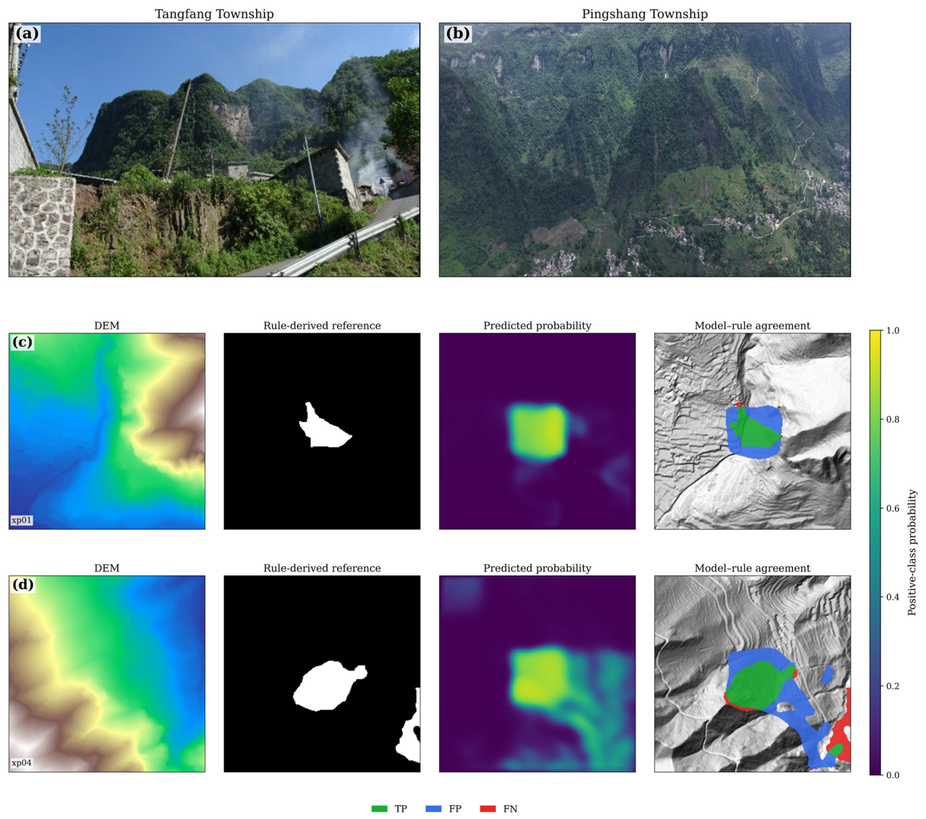
Author Contributions

Conceptualization, B.D. and X.M.; methodology, X.M. and J.Y.; software, X.M.; validation, J.Y.; formal analysis, Y.Y.; investigation, B.D.; resources, Y.Y.; data curation, B.D.; writing—original draft preparation, X.M.; writing—review and editing, X.M.; visualization, J.Y.; supervision, B.T.; project administration, Y.Y.; funding acquisition, B.D. All authors have read and agreed to the published version of the manuscript.

Funding

This work was supported by Research on Major Landslide Failure Mechanism and Risk Control in the Wumeng Mountain Region (No. 202403AA080001), the National Natural Science Foundation of Hebei Province (No. E2024210157), the National Natural Science Foundation of China (No. U2469205), the New Cornerstone Science Foundation through the XPLORER PRIZE, and the Fundamental and Interdisciplinary Disciplines Breakthrough Plan of the Ministry of Education of China (No. JYB2025XDXM104).

Data Availability Statement

Restrictions apply to the availability of the raw data used in this study. The airborne LiDAR DEM, slope-unit boundaries, and profile-line data were obtained from China Institute of Geo-Environment Monitoring and are available from the corresponding author with the permission of the data provider. The processed data supporting the findings of this study may be made available by the corresponding author upon reasonable request, subject to approval from the data provider.

Acknowledgments

During the preparation of this manuscript, the authors used Claude Sonnet 4.5 (Anthropic) and ChatGPT (GPT-5.6 Sol, OpenAI) for the purposes of manuscript drafting assistance, language editing, structural revision, and improving textual clarity. The authors reviewed and edited the output and take full responsibility for the content of this publication.

Conflicts of Interest

The authors declare no conflicts of interest.

Abbreviations

The following abbreviations are used in this manuscript:
DEMDigital Elevation Model
EPSGEuropean Petroleum Survey Group
ASPPAtrous Spatial Pyramid Pooling
CNNConvolutional Neural Network
LiDARLight Detection and Ranging
MLPMulti-Layer Perceptron

References

  1. Froude, M.J.; Petley, D.N. Global Fatal Landslide Occurrence from 2004 to 2016. Nat. Hazards Earth Syst. Sci. 2018, 18, 2161–2181. [Google Scholar] [CrossRef] [Scilit]
  2. Huang, R.; Li, W. Post-Earthquake Landsliding and Long-Term Impacts in the Wenchuan Earthquake Area, China. Eng. Geol. 2014, 182, 111–120. [Google Scholar] [CrossRef] [Scilit]
  3. Fan, X.; Scaringi, G.; Korup, O.; West, A.J.; van Westen, C.J.; Tanyas, H.; Hovius, N.; Hales, T.C.; Jibson, R.W.; Allstadt, K.E.; et al. Earthquake-Induced Chains of Geologic Hazards: Patterns, Mechanisms, and Impacts. Rev. Geophys. 2019, 57, 421–503. [Google Scholar] [CrossRef] [Scilit]
  4. Wu, M.; Li, A.; Li, Z.; Chen, N.; Tian, S.; Hou, R.; Habumugisha, J.M.; Huang, N. Frost-Heaving May Triggered the Catastrophic Landslide in Zhenxiong on January 22, 2024. Landslides 2025, 22, 1153–1166. [Google Scholar] [CrossRef] [Scilit]
  5. Fell, R.; Corominas, J.; Bonnard, C.; Cascini, L.; Leroi, E.; Savage, W.Z. Guidelines for Landslide Susceptibility, Hazard and Risk Zoning for Land Use Planning. Eng. Geol. 2008, 102, 85–98. [Google Scholar] [CrossRef] [Scilit]
  6. Guzzetti, F.; Mondini, A.C.; Cardinali, M.; Fiorucci, F.; Santangelo, M.; Chang, K.-T. Landslide Inventory Maps: New Tools for an Old Problem. Earth-Sci. Rev. 2012, 112, 42–66. [Google Scholar] [CrossRef] [Scilit]
  7. Cruden, D.M.; Varnes, D.J. Landslide Types and Processes. In Landslides: Investigation and Mitigation; Turner, A.K., Schuster, R.L., Eds.; National Academy Press: Washington, DC, USA, 1996; pp. 36–75. [Google Scholar]
  8. Reichenbach, P.; Rossi, M.; Malamud, B.D.; Mihir, M.; Guzzetti, F. A Review of Statistically-Based Landslide Susceptibility Models. Earth-Sci. Rev. 2018, 180, 60–91. [Google Scholar] [CrossRef] [Scilit]
  9. Merghadi, A.; Yunus, A.P.; Dou, J.; Whiteley, J.; ThaiPham, B.; Bui, D.T.; Avtar, R.; Abderrahmane, B. Machine Learning Methods for Landslide Susceptibility Studies: A Comparative Overview of Algorithm Performance. Earth-Sci. Rev. 2020, 207, 103225. [Google Scholar] [CrossRef] [Scilit]
  10. Ayalew, L.; Yamagishi, H. The Application of GIS-Based Logistic Regression for Landslide Susceptibility Mapping in the Kakuda-Yahiko Mountains, Central Japan. Geomorphology 2005, 65, 15–31. [Google Scholar] [CrossRef] [Scilit]
  11. Yao, X.; Tham, L.G.; Dai, F.C. Landslide Susceptibility Mapping Based on Support Vector Machine: A Case Study on Natural Slopes of Hong Kong, China. Geomorphology 2008, 101, 572–582. [Google Scholar] [CrossRef] [Scilit]
  12. Catani, F.; Lagomarsino, D.; Segoni, S.; Tofani, V. Landslide Susceptibility Estimation by Random Forests Technique: Sensitivity and Scaling Issues. Nat. Hazards Earth Syst. Sci. 2013, 13, 2815–2831. [Google Scholar] [CrossRef] [Scilit]
  13. Prakash, N.; Manconi, A.; Loew, S. Mapping Landslides on EO Data: Performance of Deep Learning Models vs. Traditional Machine Learning Models. Remote Sens. 2020, 12, 346. [Google Scholar] [CrossRef] [Scilit]
  14. Mohan, A.; Singh, A.K.; Kumar, B.; Dwivedi, R. Review on Remote Sensing Methods for Landslide Detection Using Machine and Deep Learning. Trans. Emerg. Telecommun. Technol. 2021, 32, e3998. [Google Scholar] [CrossRef] [Scilit]
  15. Ronneberger, O.; Fischer, P.; Brox, T. U-Net: Convolutional Networks for Biomedical Image Segmentation. In Proceedings of the MICCAI, Munich, Germany, 5–9 October 2015; pp. 234–241. [Google Scholar] [CrossRef] [Scilit]
  16. Chen, L.-C.; Zhu, Y.; Papandreou, G.; Schroff, F.; Adam, H. Encoder-Decoder with Atrous Separable Convolution for Semantic Image Segmentation. In Proceedings of the ECCV, Munich, Germany, 8–14 September 2018; pp. 833–851. [Google Scholar] [CrossRef] [Scilit]
  17. Xie, E.; Wang, W.; Yu, Z.; Anandkumar, A.; Alvarez, J.M.; Luo, P. SegFormer: Simple and Efficient Design for Semantic Segmentation with Transformers. In Proceedings of the NeurIPS, Virtual, 6–14 December 2021; pp. 12077–12090. [Google Scholar] [CrossRef] [Scilit]
  18. Huang, R.; Chen, T. Landslide Recognition from Multi-Feature Remote Sensing Data Based on Improved Transformers. Remote Sens. 2023, 15, 3340. [Google Scholar] [CrossRef] [Scilit]
  19. Chen, Z.; Zhang, Y.; Ouyang, C.; Zhang, F.; Ma, J. Automated Landslides Detection for Mountain Cities Using Multi-Temporal Remote Sensing Imagery. Sensors 2018, 18, 821. [Google Scholar] [CrossRef] [Scilit] [PubMed]
  20. Ji, S.; Yu, D.; Shen, C.; Li, W.; Xu, Q. Landslide Detection from an Open Satellite Imagery and Digital Elevation Model Dataset Using Attention Boosted Convolutional Neural Networks. Landslides 2020, 17, 1337–1352. [Google Scholar] [CrossRef] [Scilit]
  21. Wu, L.; Liu, R.; Ju, N.; Zhang, A.; Gou, J.; He, G.; Lei, Y. Landslide Mapping Based on a Hybrid CNN-Transformer Network and Deep Transfer Learning Using Remote Sensing Images with Topographic and Spectral Features. Int. J. Appl. Earth Obs. Geoinf. 2024, 126, 103612. [Google Scholar] [CrossRef] [Scilit]
  22. Jin, Y.; Liu, X.; Huang, X. EMR-HRNet: A Multi-Scale Feature Fusion Network for Landslide Segmentation from Remote Sensing Images. Sensors 2024, 24, 3677. [Google Scholar] [CrossRef] [Scilit] [PubMed]
  23. Zhou, N.; Hong, J.; Cui, W.; Wu, S.; Zhang, Z. A Multiscale Attention Segment Network-Based Semantic Segmentation Model for Landslide Remote Sensing Images. Remote Sens. 2024, 16, 1712. [Google Scholar] [CrossRef] [Scilit]
  24. Chen, X.; Zhao, C.; Xi, J.; Lu, Z.; Ji, S.; Chen, L. Deep Learning Method of Landslide Inventory Map with Imbalanced Samples in Optical Remote Sensing. Remote Sens. 2022, 14, 5517. [Google Scholar] [CrossRef] [Scilit]
  25. Li, D.; Tang, X.; Tu, Z.; Fang, C.; Ju, Y. Automatic Detection of Forested Landslides: A Case Study in Jiuzhaigou County, China. Remote Sens. 2023, 15, 3850. [Google Scholar] [CrossRef] [Scilit]
  26. Ghorbanzadeh, O.; Blaschke, T.; Gholamnia, K.; Meena, S.R.; Tiede, D.; Aryal, J. Evaluation of Different Machine Learning Methods and Deep-Learning Convolutional Neural Networks for Landslide Detection. Remote Sens. 2019, 11, 196. [Google Scholar] [CrossRef] [Scilit]
  27. Steger, S.; Mair, V.; Kofler, C.; Pittore, M.; Zebisch, M.; Schneiderbauer, S. Correlation Does Not Imply Geomorphic Causation in Data-Driven Landslide Susceptibility Modelling—Benefits of Exploring Landslide Data Collection Effects. Sci. Total Environ. 2021, 776, 145935. [Google Scholar] [CrossRef] [Scilit] [PubMed]
  28. Jaboyedoff, M.; Oppikofer, T.; Abellan, A.; Derron, M.-H.; Loye, A.; Metzger, R.; Pedrazzini, A. Use of LIDAR in Landslide Investigations: A Review. Nat. Hazards 2012, 61, 5–28. [Google Scholar] [CrossRef] [Scilit]
  29. Liu, X.; Peng, Y.; Lu, Z.; Li, W.; Yu, J.; Ge, D.; Xiang, W. Feature-Fusion Segmentation Network for Landslide Detection Using High-Resolution Remote Sensing Images and Digital Elevation Model Data. IEEE Trans. Geosci. Remote Sens. 2023, 61, 4500314. [Google Scholar] [CrossRef] [Scilit]
  30. Alvioli, M.; Marchesini, I.; Reichenbach, P.; Rossi, M.; Ardizzone, F.; Fiorucci, F.; Guzzetti, F. Automatic Delineation of Geomorphological Slope Units with r.slopeunits v1.0 and Their Optimization for Landslide Susceptibility Modeling. Geosci. Model Dev. 2016, 9, 3975–3991. [Google Scholar] [CrossRef] [Scilit]
  31. Schlögel, R.; Marchesini, I.; Alvioli, M.; Reichenbach, P.; Rossi, M.; Malet, J.-P. Optimizing Landslide Susceptibility Zonation: Effects of DEM Spatial Resolution and Slope Unit Delineation on Logistic Regression Models. Geomorphology 2018, 301, 10–20. [Google Scholar] [CrossRef] [Scilit]
  32. Ba, Q.; Chen, Y.; Deng, S.; Yang, J.; Li, H. A Comparison of Slope Units and Grid Cells as Mapping Units for Landslide Susceptibility Assessment. Earth Sci. Inform. 2018, 11, 373–388. [Google Scholar] [CrossRef] [Scilit]
  33. Wang, X.; Du, A.; Hu, F.; Liu, Z.; Zhang, X.; Wang, L.; Guo, H. Landslide Susceptibility Evaluation Based on Active Deformation and Graph Convolutional Network Algorithm. Front. Earth Sci. 2023, 11, 1132722. [Google Scholar] [CrossRef] [Scilit]
  34. Xue, Z.; Xu, C.; Zhang, Z.; Feng, L.; Li, H.; Zhang, H.; Zhu, D.; Sun, J.; Wang, P.; Li, L.; et al. Inventory of Landslide Relics in Zhenxiong County Based on Human-Machine Interactive Visual Interpretation, Yunnan Province, China. Front. Earth Sci. 2025, 12, 1518377. [Google Scholar] [CrossRef] [Scilit]
  35. Gillies, S. Rasterio: Geospatial Raster I/O for Python Programmers. Available online: https://rasterio.readthedocs.io (accessed on 15 April 2025).
  36. He, K.; Zhang, X.; Ren, S.; Sun, J. Deep Residual Learning for Image Recognition. In Proceedings of the CVPR, Las Vegas, NV, USA, 27–30 June 2016; pp. 770–778. [Google Scholar] [CrossRef] [Scilit]
  37. Zhou, Z.; Rahman Siddiquee, M.M.; Tajbakhsh, N.; Liang, J. UNet++: A Nested U-Net Architecture for Medical Image Segmentation. In Deep Learning in Medical Image Analysis and Multimodal Learning for Clinical Decision Support; Springer: Cham, Switzerland, 2018; pp. 3–11. [Google Scholar] [CrossRef] [Scilit] [PubMed]
  38. Milletari, F.; Navab, N.; Ahmadi, S.-A. V-Net: Fully Convolutional Neural Networks for Volumetric Medical Image Segmentation. In Proceedings of the 3DV, Stanford, CA, USA, 25–28 October 2016; pp. 565–571. [Google Scholar] [CrossRef] [Scilit]
  39. Lin, T.-Y.; Goyal, P.; Girshick, R.; He, K.; Dollár, P. Focal Loss for Dense Object Detection. In Proceedings of the ICCV, Venice, Italy, 22–29 October 2017; pp. 318–327. [Google Scholar] [CrossRef] [Scilit]
  40. Roberts, D.R.; Bahn, V.; Ciuti, S.; Boyce, M.S.; Elith, J.; Guillera-Arroita, G.; Hauenstein, S.; Lahoz-Monfort, J.J.; Schröder, B.; Thuiller, W.; et al. Cross-Validation Strategies for Data with Temporal, Spatial, Hierarchical, or Phylogenetic Structure. Ecography 2017, 40, 913–929. [Google Scholar] [CrossRef] [Scilit]
  41. Loshchilov, I.; Hutter, F. Decoupled Weight Decay Regularization. In Proceedings of the ICLR, New Orleans, LA, USA, 6–9 May 2019. [Google Scholar] [CrossRef] [Scilit]
Figure 1. (a) Location of Yunnan Province within China; (b) location of Zhenxiong County and the four LiDAR-covered study subregions; and (c) annotated field photograph illustrating the steep-upper–gentle-lower terrain morphology that motivated the boot-shaped screening concept.
Remotesensing 18 02983 g001
Figure 2. Overall workflow of the proposed two-stage framework. Stage 1 generates rule-derived boot-shaped terrain candidate masks through hydrology-based slope-unit delineation, representative-profile construction, and geomorphological screening. Stage 2 evaluates DEM-derived raster inputs and semantic segmentation models using the rule-derived masks as supervision. The final surrogate uses DEM and slope-gradient rasters to produce candidate probability maps, and model performance is evaluated as agreement with the rule-derived reference masks.
Remotesensing 18 02983 g002
Figure 3. Characteristics of the rule-derived patch dataset. (a) Distribution of the reference-positive pixel ratio among positive patches; (b) distribution of positive and reference-negative patches across the four study subregions; and (c) distribution of the number of reference-positive pixels per positive patch.
Remotesensing 18 02983 g003
Figure 4. Representative visualization of the terrain variables considered in the input-design experiments and their corresponding rule-derived reference masks. Columns show (a) DEM elevation, (b) slope gradient, (c) sine-transformed aspect, (d) cosine-transformed aspect, and (e) the rule-derived reference mask.
Remotesensing 18 02983 g004
Figure 5. Qualitative overview of the terrain context and illustrative model predictions. (a) Ground-based view of the mountainous terrain in Tangfang Township and (b) aerial view of the mountainous landscape in Pingshang Township, provided as geomorphological context for the study area. The photographs are not used as independent validation of the rule-derived reference masks or model predictions. (c,d) Two illustrative positive examples from the held-out test partition of the final DeepLabV3+ configuration using DEM and slope as input features and Dice + Focal as the loss function.
Remotesensing 18 02983 g005
Figure 6. Sensitivity of the rule-derived candidate definition and downstream model–rule agreement across nine profile-parameter configurations. (a) Pixel-level F1-score (mean ± SD across three spatial folds) for each parameter configuration. (b) Global Jaccard overlap with the predefined reference configuration T2 and the corresponding candidate-area ratio relative to T2.
Remotesensing 18 02983 g006
Figure 7. Whole-area precision–recall curves under natural rule-derived candidate prevalence for the four held-out subregions: (a) xp01, (b) xp02, (c) xp04, and (d) xp05. Curves correspond to the three stochastic seed models for each LOSO setting. Dashed horizontal lines indicate the reference-positive prevalence of each complete held-out subregion. AUPRC values are reported as mean ± SD across the three seed models.
Remotesensing 18 02983 g007
Table 1. Properties of the airborne LiDAR DEM data for the four study subregions.
RegionRaster Size (Rows × Cols)Valid LiDAR-Covered Area (km2)Elevation Range (m)Slope-Gradient Range (°)Valid DEM Pixels (%)
xp016147 × 457453.321525–23240–87.647.4
xp027491 × 652573.29989–19480–88.337.5
xp041878 × 269412.001379–21130–84.759.3
xp051892 × 22908.621405–20790–82.549.7
Table 2. Model-specific optimization and early-stopping settings used in the architecture comparison.
ModelInitial. LRBatch SizeWarmup EpochsPatienceWeight
Decay
Max
Epochs
DeepLabV3+5 × 10−41210151 × 10−4200
U-Net5 × 10−41615255 × 10−4200
U-Net++1 × 10−31210151 × 10−4200
SegFormer-B03 × 10−5820305 × 10−2200
Table 3. Quantitative comparison of the four segmentation architectures under the common DEM + slope-gradient and Dice + Focal configuration. Values are descriptive mean ± SD across the nine fold–seed evaluations (three spatial folds × three random seeds); statistical inference was conducted at the spatial-fold level.
ModelPatch-F1 I o U + mIoUF1PrecisionRecall
DeepLabV3+0.814 ± 0.1450.214 ± 0.0260.557 ± 0.0140.351 ± 0.0360.328 ± 0.0320.394 ± 0.088
U-Net0.764 ± 0.1940.150 ± 0.0360.511 ± 0.0240.259 ± 0.0540.228 ± 0.0480.355 ± 0.147
U-Net++0.752 ± 0.1850.129 ± 0.0350.488 ± 0.0520.226 ± 0.0570.204 ± 0.0670.348 ± 0.161
SegFormer-B00.624 ± 0.1650.063 ± 0.0260.422 ± 0.0960.118 ± 0.0460.132 ± 0.0560.223 ± 0.186
Table 4. Performance of DeepLabV3+ under six terrain-input configurations. Aspect is represented jointly by its sine and cosine components. Values are descriptive mean ± SD across the nine fold–seed evaluations (three spatial folds × three random seeds); statistical inference was conducted at the spatial-fold level.
Input ChannelsPatch-F1IoU+mIoUF1PrecisionRecall
DEM0.649 ±0.1790.127 ± 0.0350.497 ± 0.0540.225 ± 0.0550.259 ± 0.1380.278 ± 0.101
Slope0.837 ± 0.1180.209 ± 0.0360.548 ± 0.0320.344 ± 0.0510.296 ± 0.0590.428 ± 0.072
DEM + Slope0.814 ± 0.1450.214 ± 0.0260.557 ± 0.0140.351 ± 0.0360.328 ± 0.0320.394 ± 0.088
DEM + Aspect (sin + cos)0.580 ± 0.2390.100 ± 0.0440.435 ± 0.1220.179 ± 0.0720.202 ± 0.1400.338 ± 0.229
Slope + Aspect (sin + cos)0.836 ± 0.0770.219 ± 0.0290.563 ± 0.0280.358 ± 0.0390.360 ± 0.0620.375 ± 0.094
DEM + Slope +Aspect (sin + cos)0.820 ± 0.0890.197 ± 0.0280.545 ± 0.0300.328 ± 0.0400.308 ± 0.0430.368 ± 0.092
Table 5. Performance of DeepLabV3+ under six loss functions using the DEM + slope-gradient input. Values are descriptive mean ± SD across the nine fold–seed evaluations (three spatial folds × three random seeds); statistical inference was conducted at the spatial-fold level.
Loss FunctionPrecisionRecallF1 I o U + mIoUPatch-F1
Dice + Focal0.328 ± 0.0320.394 ± 0.0880.351 ± 0.0360.214 ± 0.0260.557 ± 0.0140.814 ± 0.145
Weighted Cross-Entropy0.262 ± 0.0400.496 ± 0.1340.333 ± 0.0580.201 ± 0.0400.532 ± 0.0200.813 ± 0.130
Dice + Cross-Entropy0.314 ± 0.0770.337 ± 0.1360.309 ± 0.0710.185 ± 0.0490.540 ± 0.0460.831 ± 0.051
Dice0.258 ± 0.0950.380 ± 0.0630.297 ± 0.0700.176 ± 0.0460.526 ± 0.0320.731 ± 0.183
Cross-Entropy0.292 ± 0.1180.335 ± 0.1480.275 ± 0.1000.163 ± 0.0680.502 ± 0.1060.743 ± 0.125
Focal0.188 ± 0.0540.274 ± 0.1530.198 ± 0.0650.111 ± 0.0410.489 ± 0.0190.615 ± 0.209
Table 6. Sensitivity of the rule-derived candidate definition and downstream model–rule agreement across nine profile-parameter configurations. n p o s denotes the number of reference-positive patches generated under each configuration; T2 (45°, 30°, 0.6) is the predefined reference configuration.
IDθupperθlowerRatioPositive Patches, n p o s F1 I o U + Jaccard vs. Ref.Area Ratio
T140°30°0.66640.247 ± 0.1210.144 ± 0.0760.2953.394
T245°30°0.62070.377 ± 0.0180.232 ±0.0131.0001.000
T350°30°0.6420.051 ± 0.0240.026 ± 0.0130.1750.175
T445°25°0.61090.261 ± 0.0650.151 ±0.0420.5610.561
T545°35°0.63110.391 ± 0.0240.243 ± 0.0180.6831.463
T645°30°0.52610.315 ± 0.0370.187 ± 0.0260.4511.377
T745°30°0.71600.332 ± 0.0980.202 ± 0.0700.4460.721
T840°25°0.54240.273 ± 0.1080.161 ± 0.0730.1112.278
T950°35°0.7450.068 ± 0.0470.035 ± 0.0260.0450.172
Table 7. Leave-one-subregion-out evaluation of the final DeepLabV3+ configuration across the four held-out study subregions.
Held-Out RegionF1mIoUPatch-F1PrecisionRecall I o U +
xp010.342 ± 0.0040.558 ± 0.0020.842 ± 0.0430.500 ± 0.0430.261 ± 0.0150.206 ± 0.003
xp020.323 ± 0.0150.543 ± 0.0090.840 ± 0.0610.256 ± 0.0200.440 ± 0.0360.193 ± 0.010
xp040.303 ± 0.0510.498 ± 0.0520.886 ± 0.0340.205 ± 0.0480.614 ± 0.1060.179 ± 0.035
xp050.319 ± 0.0200.537 ± 0.0130.870 ± 0.0000.289 ± 0.0350.359 ± 0.0310.190 ± 0.013
Macro mean0.321 ± 0.0160.534 ± 0.0260.860 ± 0.0220.312 ± 0.1290.419 ± 0.1500.192 ± 0.011
Note: Region-level values are descriptive mean ± SD across three stochastic seeds evaluated on the same held-out subregion. The macro mean is calculated from the four region-level means, and the accompanying SD describes variability among the four held-out subregions rather than among 12 independent geographic replicates. All metrics quantify agreement with rule-derived reference masks.
Table 8. Whole-area model–rule agreement under natural candidate prevalence using fixed and validation-derived operating thresholds. Region-level values are reported as mean ± SD across three stochastic seeds.
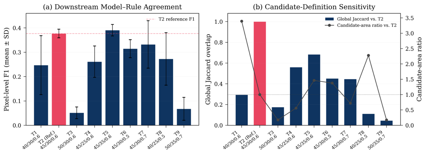
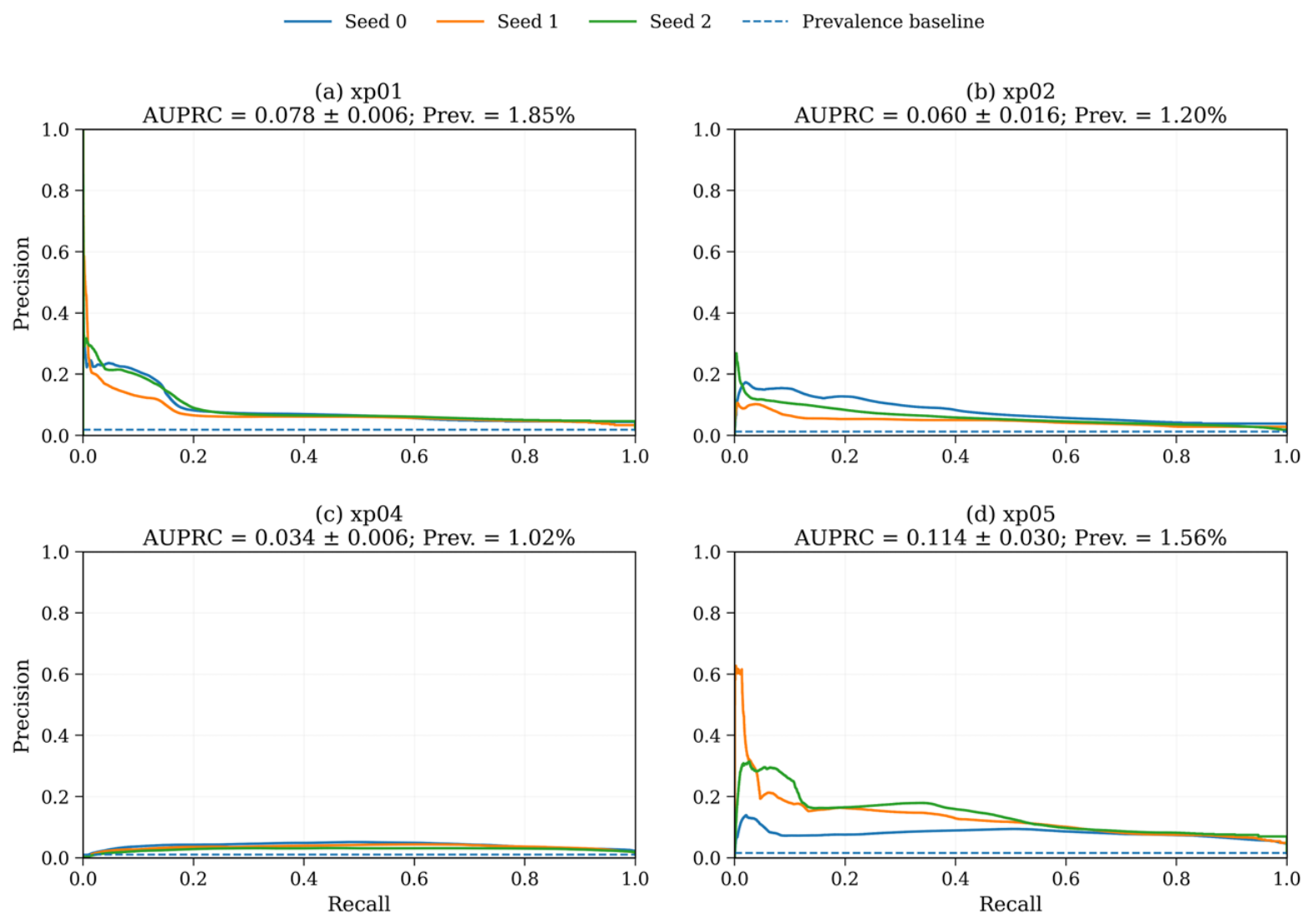
RegionRef. Prevalence (%)AUPRC t v a l F1@0.5F1@ t v a l Δ F1 I o U + @ 0.5 I o U + @ t v a l
xp011.8540.078 ± 0.0060.327 ± 0.0550.021 ± 0.0060.109 ± 0.045+0.0890.010 ± 0.0030.058 ± 0.025
xp021.2040.060 ± 0.0160.643 ± 0.1680.109 ± 0.0290.085 ± 0.063−0.0250.058 ± 0.0160.045 ± 0.034
xp041.0230.034 ± 0.0060.450 ± 0.0700.043 ± 0.0300.057 ± 0.009+0.0140.022 ± 0.0160.029 ± 0.005
xp051.5590.114 ± 0.0300.377 ± 0.3230.117 ± 0.0400.131 ± 0.109+0.0140.063 ± 0.0220.072 ± 0.061
Macro mean1.4100.072 ± 0.0340.449 ± 0.1390.072 ± 0.0480.095 ± 0.032+0.0230.038 ± 0.0260.051 ± 0.018
Note: The macro mean was calculated from the four region-level means, and the accompanying SD describes variability among the four held-out subregions rather than among 12 independent geographic replicates. t v a l denotes the operating threshold selected from the corresponding LOSO validation split. All performance metrics quantify agreement with rule-derived reference masks.
Disclaimer/Publisher’s Note: The statements, opinions and data contained in all publications are solely those of the individual author(s) and contributor(s) and not of MDPI and/or the editor(s). MDPI and/or the editor(s) disclaim responsibility for any injury to people or property resulting from any ideas, methods, instructions or products referred to in the content.