HDSMNet: Height-Guided Sparse Cross-Modal Fusion for High-Resolution Remote Sensing Semantic Segmentation

Highlights

What are the main findings?

• We propose HDSMNet for high-resolution optical–nDSM remote sensing semantic segmentation, where three nDSM-derived structural cues provide guidance for sparse cross-modal feature interaction.
• HGSCF is the principal methodological component for geometry-guided cross-modal fusion, while an adapted Context-Guided Refinement (CGR) path serves as a supplementary output refinement path. HDSMNet achieves 86.57% and 84.22% mIoU on the ISPRS Potsdam and Vaihingen datasets, respectively.

What are the implications of the main findings?

• The results indicate that nDSM should not only be treated as an auxiliary input for generic multimodal fusion, but can also provide structured geometric cues for selective optical–nDSM feature interaction in complex urban scenes.
• The findings support combining modality-specific feature extraction, height-guided sparse fusion, and output-stage contextual refinement for optical–nDSM segmentation.

Abstract

High-resolution remote sensing semantic segmentation requires the joint modeling of local details, global semantics, and height-derived geometric structures, and it provides an important basis for urban object mapping, land-cover analysis, and fine-grained spatial understanding. However, in complex urban scenes, fine-grained boundaries, small objects, inter-class similarity, and spectral confusion can still weaken the stability of pixel-level prediction. To enhance discriminative dense feature representations in high-resolution remote sensing images, we propose HDSMNet, a dual-branch multimodal semantic segmentation network designed for optical–nDSM data. The network separately extracts appearance and semantic features from optical imagery and height–structural features from nDSM, and introduces a Height-Guided Sparse Cross-Modal Fusion (HGSCF) module. Rather than treating nDSM as an additional feature source for generic fusion, HGSCF derives contextual representations, local feature contrasts, and structural-discontinuity cues from encoded nDSM features and uses them to guide sparse anchor-based interaction between optical and height features. This design enhances discriminative dense feature representations through interaction with a compact set of geometry-guided anchors. To complement HGSCF at the output stage, HDSMNet further adapts a Context-Guided Refinement (CGR) path that combines intermediate-response-guided contextual aggregation with dynamic feature modulation. This supplementary path recalibrates decoder features for output refinement. Experiments on the ISPRS Potsdam and Vaihingen datasets show that HDSMNet achieves mIoU values of 86.57% and 84.22%, respectively; ablation results further identify HGSCF as the main contributor to the observed improvement.

1. Introduction

High-resolution remote sensing semantic segmentation provides important technical support for urban object mapping, land-cover monitoring, and fine-grained spatial analysis. Remote sensing data have been widely used in urban planning and ecological assessment [1], and they also play a sustained role in agricultural monitoring and related applications [2]. In these applications, semantic segmentation assigns a semantic label to each pixel and is therefore one of the fundamental tasks in the intelligent interpretation of remote sensing imagery [3]. However, high-resolution urban imagery not only provides richer spatial details but also amplifies challenges such as scale variation, intra-class diversity, inter-class similarity, shadow occlusion, and fragmented boundaries. Diakogiannis et al. noted that high-resolution remote sensing segmentation needs to handle complex object geometries and pronounced class differences [4], while Wang et al. further emphasized the importance of jointly modeling global semantics and local details [5]. Therefore, models for high-resolution remote sensing semantic segmentation should not only produce accurate pixel-level labels, but also extract dense feature representations that support the discrimination of fine boundaries, small objects, and confusing regions.

Advances in computer vision have substantially promoted semantic segmentation. FCN established an end-to-end pixel-level prediction paradigm [6], and U-Net improved spatial detail recovery through an encoder–decoder structure with skip connections [7]. CNN-based methods provide useful local inductive biases for extracting textures, edges, and morphology, but their local receptive fields limit the modeling of large-scale semantic relationships. DeepLabv3+ introduced multiscale context aggregation through atrous convolution and decoder refinement [8], while PSPNet enlarged scene-level context through pyramid pooling [9]. Transformer-based models further use self-attention to capture long-range dependencies, as demonstrated by ViT [10] and Swin Transformer [11]. Mamba offers an efficient state-space route for long-range sequence modeling [12], and VMamba extends this idea to visual feature maps [13]. These developments strengthen feature extraction from optical imagery, including local detail recovery, contextual reasoning, and global representation. However, the resulting dense features are still dominated by two-dimensional appearance cues and cannot directly encode height-derived structures. This limitation can lead to unstable pixel-level discrimination in spectrally similar regions, such as buildings and impervious surfaces, trees and low vegetation, or cars and road backgrounds.

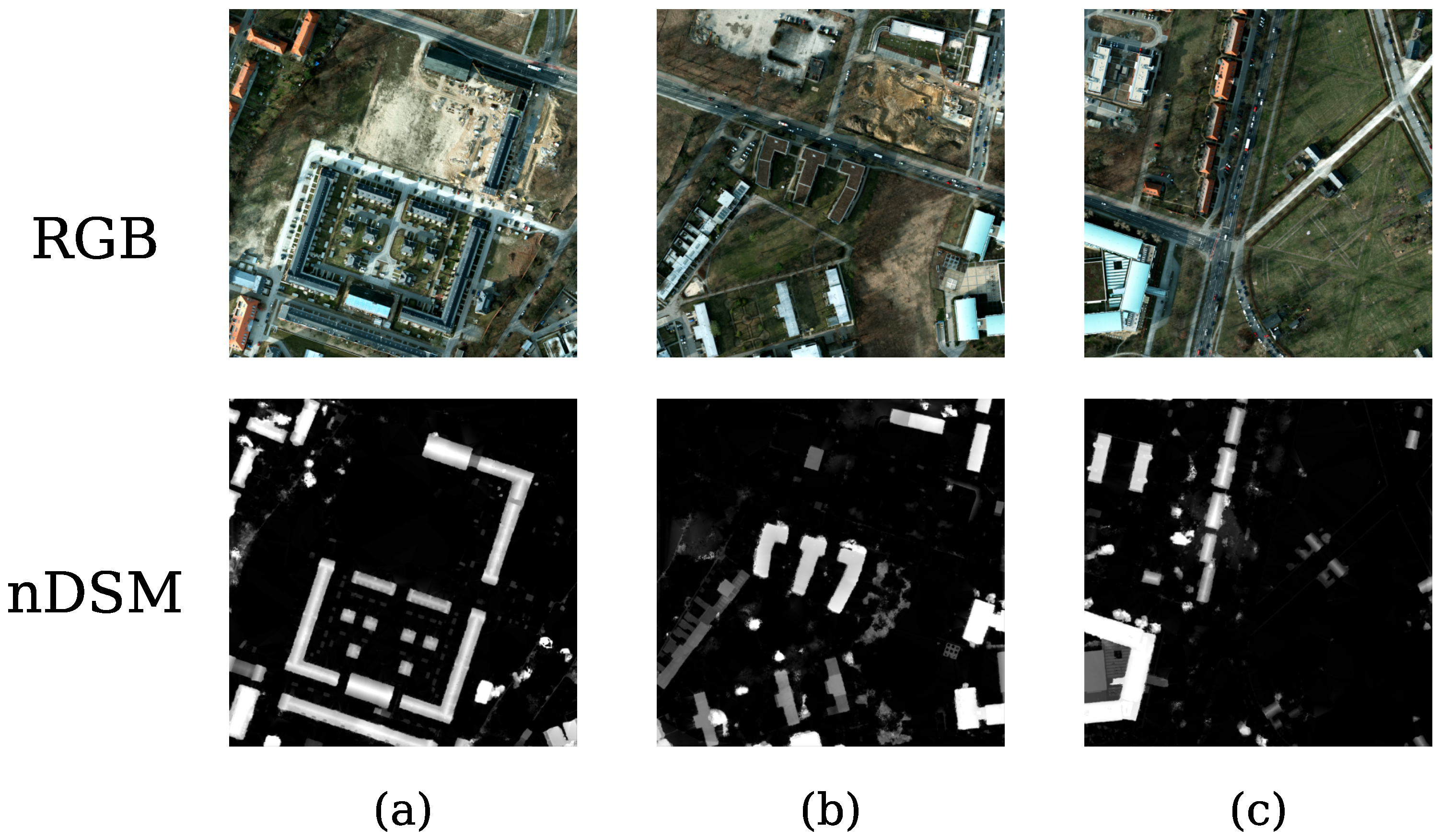
Multimodal optical–DSM fusion is therefore a natural way to introduce complementary geometric information. As shown in Figure 1, optical imagery provides color, texture, and architectural details, whereas digital surface models (DSMs) and their normalized form, normalized digital surface models (nDSMs), describe height variations, local height differences, and structural boundaries. Although optical imagery and nDSM share the same raster format, they describe different physical properties. Optical imagery mainly records spectral and radiometric responses in addition to surface appearance, whereas nDSM is derived from elevation data and represents relative object height and three-dimensional geometric structure. Therefore, we treat optical imagery and nDSM as heterogeneous modalities in this study. FuseNet demonstrated the value of depth cues for RGB-D segmentation [14], and CMFNet extended cross-modal multiscale fusion to remote sensing data [15]. FTransUNet strengthens long-range inter-modal interaction through multilevel fusion [16], and FTransDeepLab improves feature alignment through rectification and cross-attention [17]. Recent works also explore feature compensation [18], graph reasoning with Mamba-aided interaction [19], Mamba-assisted fusion [20], multimodal state space modeling [21], and frequency-domain representation [22]. These studies confirm that height information can complement optical appearance features, but they also point to a more specific issue: elevation data should not merely be fused with optical features; its encoded structural cues should guide which cross-modal information is injected into dense representations.

Accordingly, a central question is how to perform discriminative cross-modal interaction according to height-derived geometric cues. Many fusion strategies rely on concatenation, general gating, or dense attention, but they do not always distinguish which height context, local height differences, and structural edges are useful for the current pixel-level decision. Uniform updates over all spatial locations may allow irrelevant height responses, local noise, and modality conflicts to enter the fused dense features. Dynamic sparse fusion in RGB + X interaction [23] and asymmetric cross-modal representation learning [24] suggest that selective interaction can reduce redundancy and modality imbalance. However, these designs do not directly convert the three nDSM-derived structural cues into explicit guidance for cross-modal fusion in remote sensing semantic segmentation. In addition, even enhanced fused features may still produce locally inconsistent outputs. OCR shows that object-level context can improve pixel representation consistency [25], and the Dynamic Prototype Guided head designed by Ni et al. indicates that explicit class embeddings can strengthen foreground discrimination at the output stage [26]. These observations motivate geometry-guided selective fusion as the primary design objective, with classifier-conditioned output refinement serving as a complementary step.

To address these challenges, we propose HDSMNet, a framework that integrates modality-specific feature extraction, height-guided sparse fusion, and output refinement. The optical branch adopts ConvNeXt V2 to extract textural and semantic appearance features [27], while the height branch uses a VSSMEncoder inspired by VMamba to model nDSM structural representations [13]. The central component is the Height-Guided Sparse Cross-Modal Fusion (HGSCF) module, which derives the three nDSM structural cues and uses them to guide sparse cross-modal interaction. After fusion and decoding, an adapted Context-Guided Refinement (CGR) path provides supplementary calibration of pixel-level predictions.

HDSMNet achieves mIoU values of 86.57% and 84.22% on the ISPRS Potsdam and Vaihingen datasets, respectively. Ablation experiments show that HGSCF provides the larger individual gains, while the adapted CGR component supplies smaller complementary improvements at the output stage. The main contributions are summarized as follows:

1.

We construct HDSMNet, a dual-branch framework that preserves modality-specific optical appearance and nDSM height–structural representations for high-resolution remote sensing semantic segmentation.

2.

We propose HGSCF as the main technical contribution. It derives three complementary structural cues from encoded nDSM features and uses geometry-aware gating and soft sparse anchors to guide selective cross-modal fusion.

3.

Experiments on the ISPRS Potsdam and Vaihingen datasets validate HDSMNet. Ablation studies identify HGSCF as the larger source of individual improvement and show that the adapted output refinement path supplies a smaller complementary gain.

2. Related Work

2.1. High-Resolution Remote Sensing Semantic Segmentation

High-resolution remote sensing semantic segmentation requires stable and discriminative features for pixel-level classification in complex scenes. Early methods mainly relied on handcrafted spectral, textural, shape, and contextual features with traditional classifiers or object-based analysis [3]. Deep learning shifted this process toward end-to-end hierarchical representation learning. FCN established the pixel-level prediction paradigm [6], U-Net recovered spatial details with encoder–decoder skip connections [7], DeepLabv3+ modeled multiscale context with atrous convolution and ASPP [8], and PSPNet aggregated scene-level context through pyramid pooling [9]. These methods improved pixel-level segmentation, but fine boundaries, small objects, and inter-class similarity in high-resolution urban imagery still require more discriminative feature representations.

Remote-sensing-oriented networks further strengthen local detail recovery and global context modeling. ResUNet-a integrates residual connections, atrous convolution, and multitask inference to handle intra-class variations and inter-class similarity [4], while UNetFormer jointly models global semantics and local details through global–local attention [5]. In broader visual representation learning and semantic segmentation research, ViT demonstrates the value of patch sequence modeling [10], SETR introduces a Transformer encoder for semantic segmentation [28], SegFormer improves efficiency through a hierarchical Transformer and lightweight decoder [29], and Swin Transformer constructs hierarchical visual representations with shifted-window attention [11]. However, these single-modal methods mainly learn color, texture, and spectral responses from optical imagery, without direct access to height structures and 3D spatial layouts. This motivates the incorporation of height–structural information to alleviate confusion between spectrally similar categories.

2.2. Optical–DSM Multimodal Feature Fusion

Optical–DSM multimodal fusion complements optical appearance features with height–structural information. Optical imagery describes color, texture, material, and spectral differences, whereas DSMs and nDSMs provide geometric cues such as height variations, local height differences, roof contours, and tree canopy structures. FuseNet demonstrated the complementary value of depth information for RGB-D semantic segmentation [14], and Audebert et al. showed that elevation data can improve very-high-resolution urban scene interpretation [30]. These findings motivate preserving modality-specific representations before cross-modal interaction.

Existing optical–DSM methods mainly explore input-level fusion, dual-branch encoding, and multilevel interaction. Input-level concatenation is simple, but it mixes the statistical distributions and noise patterns of different modalities. Dual-branch or middle-fusion strategies preserve modality-specific representations more effectively. CMGFNet filters DSM responses with cross-modal gating [31], G2GNet calibrates RGB features through gather-to-guide interaction [32], CIMFNet improves cross-layer fusion [33], PACSCNet enhances adjacent-scale interaction [34], and CMFNet strengthens cross-modal multiscale complementarity [15]. These methods show the value of multimodal fusion, but general gating or hierarchical interaction does not necessarily make explicit use of height context, local height differences, and structural edges.

Recent methods further enhance cross-modal interaction with Transformer modeling, graph reasoning, and feature compensation. FTransUNet models local details and global inter-modal relationships at different levels [16], FTransDeepLab improves alignment through feature rectification and cross-attention [17], and MMA-Net combines cross-layer fusion with multiscale attention [35]. CFCGNet addresses optical–DSM modality discrepancy through feature compensation and GCN-based reconstruction [18], while MGF-GCN introduces height-aware graph convolution for structural relationship modeling [19]. These studies move optical–DSM fusion from simple aggregation toward compensation, interaction, and reconstruction. However, dense attention or general relationship modeling may still propagate useful geometric cues together with redundant height responses.

2.3. Mamba/State Space Models for Feature Extraction

Mamba and state space models provide a long-range modeling route that differs from self-attention. S4 improves long-sequence modeling efficiency through structured state space parameterization [36], and Mamba introduces a selective state space mechanism for content-dependent sequence updating with linear complexity [12]. In visual tasks, Vim adopts bidirectional Mamba blocks for image patch sequences [37], and VMamba extends state space modeling to two-dimensional feature maps through selective scanning [13]. These models are attractive for large remote sensing images because they capture long-range spatial relationships with controllable computational complexity.

Remote sensing segmentation studies have introduced Mamba/SSM into both single-modal and multimodal feature extraction. RS3Mamba uses VSS blocks to provide global information for a convolutional branch [38], and AfaMamba enhances global–local representations through adaptive feature aggregation [39]. In multimodal segmentation, MFMamba uses a Mamba branch to extract DSM structural features [20], while MGF-GCN combines Mamba with graph convolution for hierarchical interaction and height–structural modeling [19]. These studies suggest that Mamba can improve long-range dependency modeling. However, long-range modeling is a feature extraction capability rather than a solution to selective cross-modal fusion by itself; it does not determine which height locations are reliable, which responses should be suppressed, or how fusion strength should vary with geometry. HDSMNet therefore adopts VSSMEncoder for nDSM feature extraction and uses HGSCF to explicitly control cross-modal interaction.

2.4. Context Modeling and Output Refinement

Output-level context modeling can improve the consistency of pixel-level predictions in high-resolution remote sensing semantic segmentation. Even after multiscale fusion, final pixel classification may still be affected by local texture noise, shadow occlusion, and boundary uncertainty. At the feature level, EDGNet uses boundary spatial information to guide multimodal fusion and integrate detailed and semantic cues across feature levels [40]. Such boundary-guided fusion enhances feature representation but does not explicitly model class-level context at the prediction stage. OCR further shows that aggregating object- or class-region context from coarse predictions can improve regional consistency and class discriminability [25]. For remote sensing categories with clear regional structures, such as buildings, roads, trees, and low vegetation, class-level context provides a useful reference for local pixel discrimination.

Existing optical–DSM methods mainly focus on dual-branch encoding, cross-modal fusion, or multiscale decoding, while class-level context at the output stage is less explicitly used. CFCGNet improves local–global reconstruction with a GCN decoder [18], MGF-GCN strengthens spatial detail recovery with a Progressive Context Cascade Decoder [19], and UNetFormer refines decoding features at the output end [5]. These designs help recover spatial details, but they do not fully exploit the class distribution implied by coarse predictions. Ni et al. designed a lightweight Dynamic Prototype Guided head to improve foreground classification through explicit class embedding [26]. Inspired by this output-stage contextual guidance idea, HDSMNet adapts classifier-conditioned contextual refinement to the output stage after height-guided optical–nDSM fusion, so that intermediate class-indexed responses can further modulate decoder features to refine pixel-level semantic predictions.

Overall, prior studies leave two complementary limitations. The primary limitation is that cross-modal fusion does not always distinguish geometry-relevant height information from redundant responses, while output-stage refinement makes limited use of class-level context. HDSMNet primarily addresses the former through HGSCF-based feature fusion, with an adapted Context-Guided Refinement component providing supplementary output refinement.

3. Materials and Methods

3.1. Overall Framework

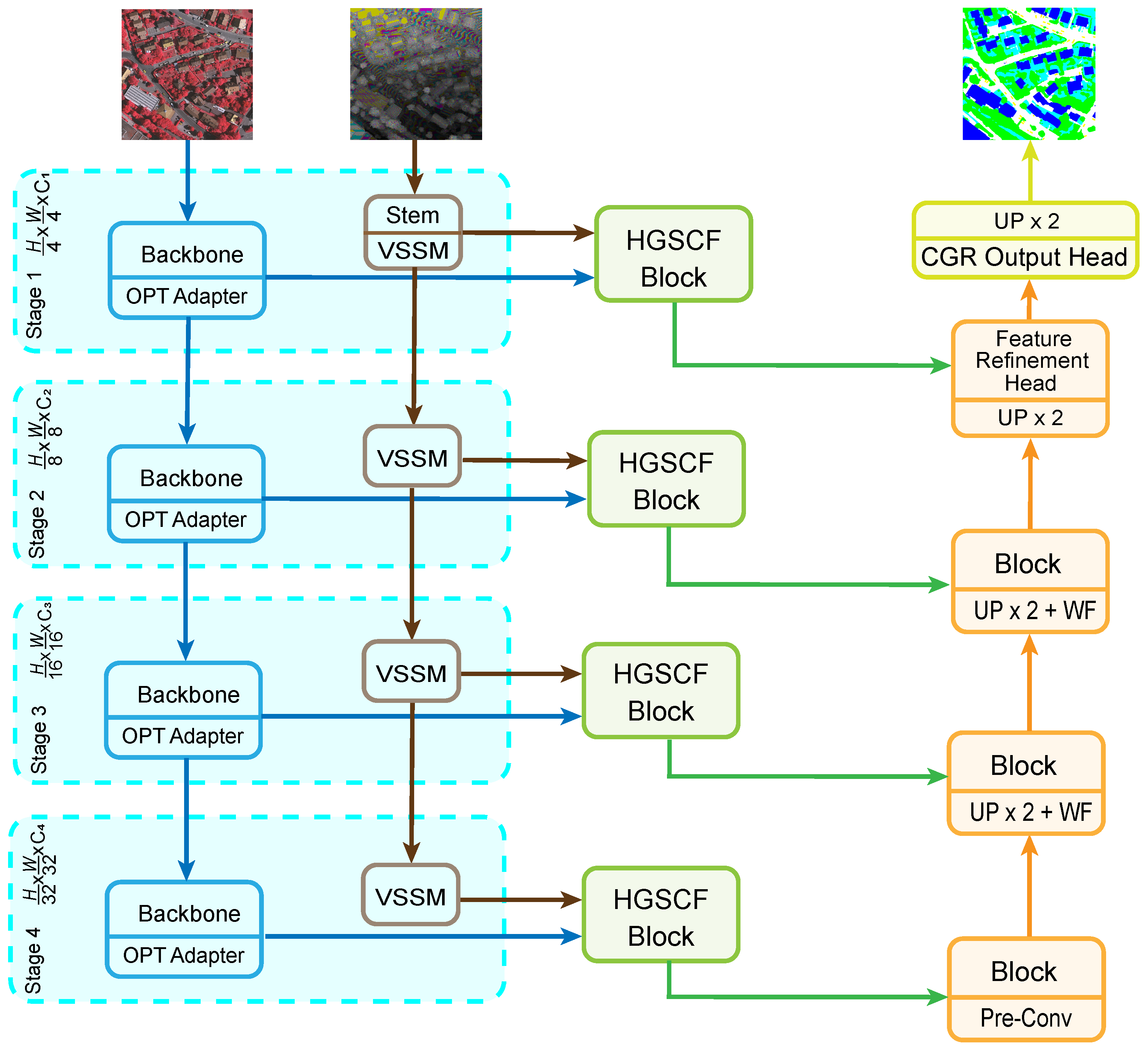
Figure 2 illustrates the overall architecture of HDSMNet. The network is designed around discriminative feature extraction and pixel-level classification for high-resolution remote sensing semantic segmentation. ConvNeXt V2 [27] extracts spectral, textural, and semantic appearance features from optical imagery, while VSSMEncoder, inspired by the visual state space modeling mechanism of VMamba [13], extracts contextual and structural representations from nDSM. HGSCF is used as the key fusion component to derive feature-space structural cues for sparse cross-modal interaction at four scales. After the decoder recovers spatial resolution, the adapted CGR path provides supplementary classifier-conditioned output refinement before final classification.

Given an optical image $X_o$ and its co-registered nDSM input $X_d$, the inputs of HDSMNet are formulated as

$$X_o\in {\mathbb{R}}^{B\times C_o\times H\times W},X_d\in {\mathbb{R}}^{B\times 1\times H\times W},$$

(1)

where B denotes the batch size, $C_o$ denotes the number of optical channels, and H and W represent the height and width of the input image, respectively. The Vaihingen dataset uses IRRG optical input, while the Potsdam dataset uses RGBIR optical input. Both datasets use nDSM as the height modality. The optical branch and the nDSM branch produce four-scale feature representations:

$$\{F_o^1,F_o^2,F_o^3,F_o^4\}=E_o\left(X_o\right),\{F_d^1,F_d^2,F_d^3,F_d^4\}=E_d\left(X_d\right),$$

(2)

where $E_o(·)$ and $E_d(·)$ denote the optical encoder and the nDSM height encoder, respectively. The optical branch focuses on preserving texture, edge, and high-level semantic information, whereas the nDSM branch emphasizes height distribution and spatial structural information. To facilitate scale-wise fusion, the two branches output four levels of features with aligned spatial resolutions, namely, ${\displaystyle \frac{H}{4}}\times {\displaystyle \frac{W}{4}}$, ${\displaystyle \frac{H}{8}}\times {\displaystyle \frac{W}{8}}$, ${\displaystyle \frac{H}{16}}\times {\displaystyle \frac{W}{16}}$, and ${\displaystyle \frac{H}{32}}\times {\displaystyle \frac{W}{32}}$. Before cross-modal fusion, each stage-wise optical feature is calibrated by a lightweight optical adapter consisting of a $1\times 1$ convolution, BatchNorm, and GELU activation:

$${\overline{F}}_o^i=\mathrm{GELU}\left(\mathrm{BN}\left({\mathrm{Conv}}_{1\times 1}(F_o^i)\right)\right).$$

(3)

This adapter organizes the stage-wise ConvNeXtV2 responses and provides stable optical representations for subsequent fusion.

At the i-th scale, HGSCF takes the adapted optical feature ${\overline{F}}_o^i$ and the height feature $F_d^i$ as inputs and produces the fused feature $F_i$:

$$F_i={\mathcal{F}}_{HGSCF}({\overline{F}}_o^i,F_d^i),i\in \{1,2,3,4\},$$

(4)

where ${\mathcal{F}}_{HGSCF}(·)$ denotes the process of height-guided sparse cross-modal fusion. The key idea is not to indiscriminately add or concatenate the two types of features, but to use the three nDSM-derived structural cues to select cross-modal information that is more discriminative for pixel-level classification. The fused features $\{F_1,F_2,F_3,F_4\}$ are then used as multiscale skip features and fed into the decoder.

Following the UNetFormer-style decoder design [5], the decoder starts from the deepest fused feature $F_4$. Global–local attention blocks jointly model window-based contextual dependencies and local spatial responses. At the intermediate stages, bilinear upsampling and learnable weighted fusion (WF) progressively combine decoder features with the corresponding multiscale skip features. Finally, a feature refinement head enhances high-resolution spatial and channel responses before the adapted CGR path. Let the decoder output feature be denoted as $F_{dec}$. The decoding process can be expressed as

$$F_{dec}=\mathcal{D}(F_1,F_2,F_3,F_4),$$

(5)

where $\mathcal{D}(·)$ denotes the multiscale skip decoding process. The supplementary CGR output refinement path then aggregates classifier-conditioned context from intermediate class-indexed responses and modulates the decoder feature:

$$\widehat{Y}={\mathcal{H}}_{CGR}\left(F_{dec}\right),$$

(6)

where ${\mathcal{H}}_{CGR}(·)$ denotes the adapted context-guided output refinement process, and $\widehat{Y}$ represents the final semantic segmentation map. Overall, HDSMNet connects optical appearance feature extraction, nDSM height–structural feature extraction, and geometry-guided cross-modal interaction, with supplementary classifier-conditioned refinement applied before pixel-level semantic classification.

3.2. Height-Guided Sparse Cross-Modal Fusion

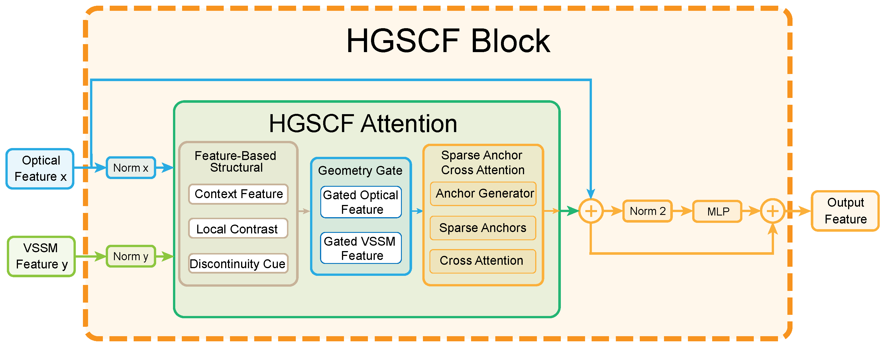
HGSCF receives optical features and nDSM features at the same scale, and its objective is to generate discriminative fused features that are more suitable for pixel-level prediction. Optical features contain rich spectral and textural responses, but they may become ambiguous in shadowed regions, occluded areas, and spectrally similar regions. Encoded nDSM features retain contextual and structural information but no longer represent raw elevation values directly. The core problem is therefore not simply how to combine the two modalities, but how to decide where and how nDSM-derived structures should guide feature injection. If the two modalities are directly concatenated, added, or fused through dense attention, complementary cues and redundant responses may be propagated simultaneously. Cai et al. reduced redundant propagation in RGB + X feature interaction through dynamic sparse fusion in the KTB framework [23], and AsymFormer proposed by Du et al. also showed that different modalities should play differentiated roles during fusion [24]. Inspired by these observations, HGSCF derives feature-space structural cues from the encoded nDSM representation and selectively updates cross-modal discriminative dense feature representations through sparse anchor-based interaction. Figure 3 shows the internal structure of this module.

Given the optical feature $X_i$ and the nDSM feature $Y_i$ at the i-th scale,

$$X_i\in {\mathbb{R}}^{B\times C_i\times h_i\times w_i},Y_i\in {\mathbb{R}}^{B\times C_i^d\times h_i\times w_i},$$

(7)

where $C_i$ and $C_i^d$ denote the numbers of optical and nDSM feature channels at this scale, respectively. HGSCF first normalizes the two types of features and maps the nDSM feature to the same channel dimension as the optical feature:

$${\widehat{X}}_i={\mathrm{Norm}}_x\left(X_i\right),{\widehat{Y}}_i={\mathrm{Norm}}_y\left(Y_i\right),Y_i^a={\varphi }_a({\widehat{Y}}_i),$$

(8)

where ${\varphi }_a(·)$ denotes a $1\times 1$ convolution for channel alignment. Because $Y_i^a$ is obtained after VSSM encoding and channel alignment, it is treated as an nDSM-derived feature representation rather than an elevation map. HGSCF therefore derives the three structural cues in this feature space. These cues are used to modulate optical and nDSM features, and sparse anchor-based interaction is further employed to generate the fusion update.

3.2.1. nDSM Feature-Based Structural Encoding

HGSCF derives three feature-space cues from the aligned nDSM representation $Y_i^a$. First, a lightweight local encoding unit consisting of a $3\times 3$ depthwise convolution, BatchNorm, and GELU activation is used to obtain a contextual feature:

$$C_i^h={\varphi }_c\left(Y_i^a\right).$$

(9)

We then characterize local variation in the aligned feature space by computing the absolute difference between each response and its local average:

$$D_i^h=\left|Y_i^a-{\mathrm{AvgPool}}_{3\times 3}\left(Y_i^a\right)\right|.$$

(10)

As $Y_i^a$ is an encoded representation, $D_i^h$ denotes local height-feature contrast rather than a physical elevation gradient. A depthwise convolution further encodes this contrast to emphasize spatially coherent discontinuity patterns:

$$E_i^h={\varphi }_e\left(D_i^h\right).$$

(11)

Accordingly, $E_i^h$ is interpreted as a structural-discontinuity-sensitive feature rather than an explicitly detected height edge. The three feature-space cues are then aggregated as

$$Z_i^h=C_i^h+D_i^h+E_i^h.$$

(12)

Although $E_i^h$ is learned from $D_i^h$, the two terms play complementary roles. $D_i^h$ directly preserves the magnitude and location of the untransformed local feature contrast, whereas $E_i^h={\varphi }_e\left(D_i^h\right)$ captures spatially coherent discontinuity patterns through a learned transformation. Their addition therefore acts as a residual refinement that retains the original contrast evidence while introducing a learned structural encoding. Together with $C_i^h$, the resulting representation combines contextual responses, local feature contrast, and encoded discontinuity patterns associated with nDSM structure. Therefore, the subsequent cross-modal interaction no longer depends only on general feature similarity, but can refer to discriminative structural cues derived from the height modality.

3.2.2. Geometry-Guided Feature Modulation

HGSCF generates geometric gating weights from the nDSM-derived feature-space cues to emphasize optical and nDSM responses related to structural patterns:

$$G_i=\sigma \left({\varphi }_g\left([Y_i^a,D_i^h,E_i^h]\right)\right),$$

(13)

where $[·]$ denotes channel-wise concatenation, and $\sigma (·)$ denotes the Sigmoid function. The gated features of the two modalities are defined as

$$X_i^g={\widehat{X}}_i\odot G_i,Y_i^g=Y_i^a\odot (1+G_i),$$

(14)

where ⊙ denotes element-wise multiplication. The gating weight $G_i$ suppresses optical responses that are weakly related to nDSM structures, while $1+G_i$ preserves the original nDSM-derived feature response and enhances locations with structural discriminability. This asymmetric formulation reflects the differentiated roles of the two modalities. The optical branch is the semantic stream to be selectively filtered, so $G_i\in [0,1]$ attenuates responses that receive weak structural support. In contrast, the nDSM branch provides the guidance used in subsequent anchor construction; using $1+G_i\in [1,2]$ forms an identity-preserving enhancement that avoids suppressing its original structural evidence when the gate value is small.

3.2.3. Sparse Anchor-Based Cross-Attention

To limit pairwise interaction to a compact context set, HGSCF uses a small number of anchors to aggregate cross-modal information. First, the geometry-modulated features are projected into a low-dimensional space:

$$Q_i=P_q\left(X_i^g\right),T_i^x=P_x\left(X_i^g\right),T_i^y=P_y\left(Y_i^g\right),$$

(15)

where $Q_i$ denotes optical queries, and $T_i^x$ and $T_i^y$ denote optical tokens and nDSM tokens, respectively. Then, the nDSM-derived structural feature and modality discrepancy are used to generate anchor weights:

$$R_i=[Z_i^h,|X_i^g-Y_i^g\left|\right],$$

(16)

$$W_i^a=\mathrm{Softmax}\left({\displaystyle \frac{{\varphi }_{anc}\left(R_i\right)}{\tau }}\right),$$

(17)

where $\tau$ is the temperature coefficient, $W_i^a\in {\mathbb{R}}^{B\times K\times N_i}$, K denotes the number of anchors, and $N_i=h_i{w}_i$. In the implementation, K is set to 16 for all HGSCF blocks, and $\tau$ is set to 0.7 to control the sharpness of anchor assignment.

The softmax in Equation (17) is applied independently over the $N_i$ spatial locations for each of the K anchors. After reshaping its last dimension to $h_i\times w_i$, $W_{i,k}^a$ forms a normalized spatial assignment map satisfying ${\sum }_{n=1}^{N_i}{W}_{i,k,n}^a=1$. Thus, an anchor is not a fixed coordinate or a hard-selected pixel, but a soft regional descriptor aggregated using weights predicted from the height-geometric representation $Z_i^h$ and the cross-modal discrepancy $|X_i^g-Y_i^g|$. The assignment need not be one-hot or spatially contiguous, allowing related responses at different locations to contribute to the same anchor. Applying the same weights to the optical and height tokens preserves their spatial correspondence before modality-adaptive fusion.

After projection and flattening, $Q_i,T_i^x,T_i^y\in {\mathbb{R}}^{B\times N_i\times d}$, where d denotes the reduced feature dimension. The anchor weights aggregate K representative anchors from $N_i$ spatial locations, producing $A_i^x,A_i^y\in {\mathbb{R}}^{B\times K\times d}$. The weights are used to aggregate anchors from the two modalities:

$$A_i^x=W_i^a{T}_i^x,A_i^y=W_i^a{T}_i^y.$$

(18)

HGSCF then computes modality weights according to the two sets of anchors and their discrepancy, and obtains the fused anchors:

$$[{\alpha }_i^x,{\alpha }_i^y]=\mathrm{Softmax}\left({\varphi }_m\left(\right[A_i^x,A_i^y,|A_i^x-A_i^y\left|\right])\right),$$

(19)

$$A_i={\alpha }_i^x\odot A_i^x+{\alpha }_i^y\odot A_i^y.$$

(20)

The softmax in Equation (19) is applied along the last dimension containing the optical and nDSM logits, so that ${\alpha }_i^x+{\alpha }_i^y=1$ for each anchor. Here, $A_i\in {\mathbb{R}}^{B\times K\times d}$ denotes the compact set of fused geometry-guided anchors. Finally, the queries and anchors are divided into M attention heads, and cross-attention is calculated independently within each head:

$$S_i={\varphi }_s\left(\underset{m=1}{\stackrel{M}{\mathrm{Concat}}}\left[\mathrm{Softmax}\left({\displaystyle \frac{Q_i^{\left(m\right)}{\left(A_i^{\left(m\right)}\right)}^{\top }}{\sqrt{d_h}}}\right)A_i^{\left(m\right)}\right]\right).$$

(21)

Here, M denotes the number of attention heads, $d_h=d/M$ is the feature dimension of each head, and ${\varphi }_s(·)$ denotes the output projection. In all experiments, the number of attention heads is set to $M=4$.

With M attention heads, each of the $N_i$ optical queries attends to K fused anchors, producing attention weights of size $B\times M\times N_i\times K$. The projected context is then restored to the $h_i\times w_i$ layout, preserving the resolution required for pixel-wise semantic prediction. The anchor aggregation and query–anchor interaction require approximately $\mathcal{O}\left(N_{i}Kd\right)$ operations, while dense global attention between two $N_i$-token sets requires $\mathcal{O}\left(N_i^{2}d\right)$; for fixed K, the anchor-weight predictor is also linear in $N_i$. Here, “sparse” denotes the use of a compact set of K key/value anchors rather than hard removal of spatial tokens. The soft assignments remain differentiable, so every location can contribute to anchor construction. Unlike dynamic sparse methods driven mainly by content similarity or hard token selection, HGSCF conditions its anchors jointly on nDSM-derived geometry and cross-modal discrepancy, making the interaction basis responsive to scene-specific height structure and modality disagreement.

3.2.4. Residual Update

HGSCF projects the sparse cross-modal context into an update term and writes it back to the optical branch through an outer residual structure:

$${\Delta }_i={\varphi }_o\left(S_i\right),$$

(22)

$${\tilde{F}}_i=X_i+{\Delta }_i,$$

(23)

$$F_i={\tilde{F}}_i+\mathrm{MLP}\left({\mathrm{Norm}}_2\left({\tilde{F}}_i\right)\right).$$

(24)

Here, ${\varphi }_o(·)$ consists of a $1\times 1$ convolution for feature organization and a $3\times 3$ depthwise convolution for projection. Through this design, HGSCF preserves the semantic representation of the optical backbone while injecting sparse cross-modal context selected by nDSM geometric structures into the fused features at each scale. The module is designed to support pixel-level discrimination of fine boundaries, small objects, and confusing regions.

3.3. Adapted Context-Guided Refinement

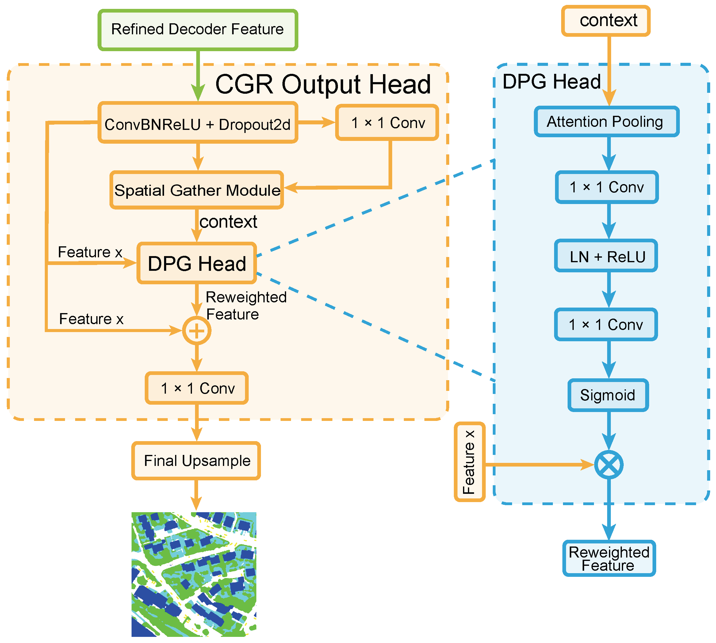
At the final pixel-level classification stage, relying only on local decoder features may still lead to inconsistent class responses. In high-resolution urban scenes, categories such as buildings and impervious surfaces, and trees and low vegetation, may have similar appearance or complex boundaries. Their local pixel responses are therefore easily affected by texture noise and boundary uncertainty. Ni et al. designed a lightweight Dynamic Prototype Guided head that uses class-context guidance for efficient semantic segmentation [26]. We adapt this idea to the decoder output produced after optical–nDSM fusion as a supplementary Context-Guided Refinement (CGR) path rather than as the main methodological contribution of HDSMNet. It uses an intermediate class-indexed response generated by a shared classifier to guide contextual aggregation, followed by dynamic modulation for refined prediction, as illustrated in Figure 4.

3.3.1. Intermediate-Response-Guided Contextual Aggregation

Let $F_{dec}$ denote the high-resolution feature output by the decoder. CGR first integrates it through a feature refinement layer consisting of ConvBNReLU and Dropout2d:

$$F_s={\varphi }_r\left(F_{dec}\right),F_s\in {\mathbb{R}}^{B\times C\times H\times W},$$

(25)

where ${\varphi }_r(·)$ denotes the feature refinement layer, and B, C, H, and W denote the batch size, channel number, height, and width, respectively. CGR then uses a shared $1\times 1$ convolution classifier to generate an intermediate class-indexed response:

$$P_c={\varphi }_{cls}\left(F_s\right),P_c\in {\mathbb{R}}^{B\times K_c\times H\times W},$$

(26)

where $K_c$ denotes the number of semantic classes, and ${\varphi }_{cls}(·)$ denotes the classification layer. The same ${\varphi }_{cls}(·)$ is reused for the final prediction rather than implemented as an independent coarse classifier. Its k-th output channel is associated with the same semantic class in both uses through the supervision applied to the final output. Although $P_c$ is not directly supervised by an auxiliary loss, gradients from the final segmentation loss propagate to it through SpatialGather, dynamic modulation, and the final classification path. Therefore, $P_c$ is treated as an internal class-indexed response rather than an independently accurate coarse segmentation prediction. SpatialGatherModule then performs classifier-conditioned weighted aggregation according to $P_c$. Specifically, the intermediate response and feature are first reshaped as

$$P_c\to {\overline{P}}_c\in {\mathbb{R}}^{B\times K_c\times N},F_s\to {\overline{F}}_s\in {\mathbb{R}}^{B\times N\times C},$$

(27)

where $N=H\times W$ denotes the total number of spatial locations. A softmax operation is then applied along the spatial dimension of each class to obtain class-specific spatial weights:

$$A_{b,k,n}={\displaystyle \frac{\exp (s·{\overline{P}}_{c,b,k,n})}{{\sum }_{n^{\prime }=1}^N\exp (s·{\overline{P}}_{c,b,k,n^{\prime }})}},$$

(28)

where s is the scaling factor. In all experiments, s is fixed at 1.0. Based on this weight, the feature ${\overline{F}}_s$ is aggregated to obtain the initial classifier-conditioned context:

$${\tilde{C}}_{cls}=A{\overline{F}}_s,$$

(29)

$${\tilde{C}}_{cls}\in {\mathbb{R}}^{B\times K_c\times C}.$$

(30)

It is then transposed and expanded as

$$C_{cls}\in {\mathbb{R}}^{B\times C\times K_c\times 1}.$$

(31)

This process can be interpreted as follows: the shared classifier provides class-indexed soft spatial responses, and SpatialGather uses them to aggregate a separate contextual descriptor for each classifier channel. These descriptors are optimized for their contribution to the final segmentation rather than as independently supervised class prototypes. Unlike ordinary global average pooling, this operation preserves the classifier-channel partition when forming the global reference.

3.3.2. Dynamic Modulation and Refined Prediction

After obtaining the classifier-conditioned context, the adapted DPG-style modulation module first performs attentive pooling on $C_{cls}$ to obtain a compact global context descriptor:

$$g=\mathcal{P}\left(C_{cls}\right),$$

(32)

where $\mathcal{P}(·)$ denotes attentive pooling, and $g\in {\mathbb{R}}^{B\times C\times 1\times 1}$. Then, g is passed through a channel modulation branch consisting of two $1\times 1$ convolutions, LayerNorm, ReLU, and Sigmoid to generate dynamic reweighting coefficients:

$$\gamma =\sigma \left({\varphi }_2\left(\delta \left({\varphi }_1\left(g\right)\right)\right)\right),$$

(33)

where ${\varphi }_1(·)$ and ${\varphi }_2(·)$ denote $1\times 1$ convolution mappings, $\delta (·)$ denotes the nonlinear transformation composed of LayerNorm and ReLU, and $\sigma (·)$ denotes the Sigmoid function. The coefficient is used to recalibrate the decoder feature along the channel dimension, while the residual form preserves the original local details:

$$F_{ref}=F_s+F_s\odot \gamma .$$

(34)

Finally, the refined feature is passed through the same shared classifier ${\varphi }_{cls}(·)$ to generate the prediction, and bilinear upsampling is used to recover the input image size:

$$P={\varphi }_{cls}\left(F_{ref}\right),$$

(35)

$$\widehat{Y}=\mathrm{Upsample}\left(P\right).$$

(36)

In summary, CGR adapts classifier-conditioned contextual aggregation to the HDSMNet output path. SpatialGather forms class-indexed contextual descriptors, and DPG-style dynamic channel modulation recalibrates the decoder features. This supplementary Context-Guided Refinement path targets residual prediction inconsistency after HGSCF-based fusion; it is not positioned as the primary methodological contribution.

3.4. Loss Function

We adopt a combination of cross-entropy loss (CE) and Dice loss as the training objective. CE loss constrains pixel-level classification, while Dice loss provides an additional region-overlap constraint and helps alleviate the training bias caused by differences in foreground category areas. The overall loss function is defined as

$$\mathcal{L}={\lambda }_{ce}{\mathcal{L}}_{ce}+{\lambda }_{dice}{\mathcal{L}}_{dice},$$

(37)

Here, ${\lambda }_{ce}$ and ${\lambda }_{dice}$ denote the weights of the two loss terms, respectively. Both ${\mathcal{L}}_{ce}$ and ${\mathcal{L}}_{dice}$ supervise the same semantic segmentation output. Therefore, Equation (37) defines a single-task training objective with two complementary loss terms rather than a multitask objective. We fix ${\lambda }_{ce}={\lambda }_{dice}=1.0$ for all experiments. This equal-weighting strategy follows common practice in semantic segmentation, allowing pixel-wise classification optimization and region-overlap optimization to contribute equally without introducing additional dataset-specific loss-weight tuning.

The two loss terms are applied only to the final prediction, and no auxiliary loss is imposed on $P_c$. The intermediate response is optimized indirectly through its differentiable contribution to the final prediction and through the shared classifier.

Let $P_{n,k}$ denote the predicted probability that pixel n belongs to class k, and let $Y_{n,k}$ denote the corresponding one-hot ground-truth label. The CE loss can be expressed as

$${\mathcal{L}}_{ce}=-{\displaystyle \frac{1}{N}}{\displaystyle \sum _{n=1}^N}{\displaystyle \sum _{k=1}^{K_c}}{Y}_{n,k}\log \left(P_{n,k}\right),$$

(38)

where N denotes the total number of valid pixels, and $K_c$ denotes the number of semantic classes. For multiclass semantic segmentation, Dice loss is computed for each valid class and then averaged:

$${\mathcal{L}}_{dice}=1-{\displaystyle \frac{1}{|{\mathcal{C}}_v|}}\sum _{c\in {\mathcal{C}}_v}{\displaystyle \frac{2{\sum }_{n=1}^N{P}_{n,c}{Y}_{n,c}+ϵ}{{\sum }_{n=1}^N{P}_{n,c}+{\sum }_{n=1}^N{Y}_{n,c}+ϵ}},$$

(39)

where ${\mathcal{C}}_v$ denotes the set of valid classes appearing in the current batch, excluding ignored pixels, and $ϵ$ is a smoothing term used to avoid division by zero. By jointly using CE and multiclass Dice loss, the training process considers both pixel-level classification constraints and region-level overlap constraints, thereby providing a relatively stable optimization objective for semantic segmentation of high-resolution remote sensing images.

4. Results

4.1. Dataset Description

4.1.1. Potsdam Dataset

The Potsdam dataset consists of 24 high-resolution true orthophotos, each with a size of $6000\times 6000$ pixels. It provides multiple spectral bands, including near-infrared, red, green, and blue bands, together with a normalized digital surface model (nDSM) at a ground sampling distance (GSD) of 5 cm. The dataset contains five foreground classes, namely, buildings (Bui.), trees (Tre.), low vegetation (Low.), cars (Car), and impervious surfaces (Imp.), in addition to one background class, namely, clutter. Following the protocol of FTransUNet [16], the 24 orthophotos are divided into 18 training images and 6 test images. The training set includes the images with indices 6_10, 7_10, 2_12, 3_11, 2_10, 7_8, 5_10, 3_12, 5_12, 7_11, 7_9, 6_9, 7_7, 4_12, 6_8, 6_12, 6_7, and 4_11, while the test set contains six images with indices 4_10, 5_11, 2_11, 3_10, 6_11, and 7_12.

4.1.2. Vaihingen Dataset

The Vaihingen dataset consists of 16 high-resolution true orthophotos, with an average image size of approximately $2500\times 2000$ pixels. Each orthophoto contains three spectral channels, namely, near-infrared (NIR), red, and green (IRRG), and is accompanied by an nDSM with a GSD of 9 cm. The foreground classes are the same as those in the Potsdam dataset, but the class distribution differs due to the different geographic scenes. Compared with Potsdam, Vaihingen contains fewer images, has a lower spatial resolution, and presents more compact urban structures, including dense buildings, complex vegetation, and fragmented road networks. Therefore, it is a challenging benchmark for semantic segmentation. Following the protocol of FTransUNet [16], the dataset is divided into a training set with 12 orthophotos and a test set with 4 orthophotos. The training set contains the images with indices 1, 3, 23, 26, 7, 11, 13, 28, 17, 32, 34, and 37, while the test set contains the images with indices 5, 21, 15, and 30.

4.2. Evaluation Metrics

We evaluate all methods using overall accuracy (OA), mean F1-score (mF1), and mean intersection over union (mIoU). OA reflects the overall classification accuracy over valid pixels, mF1 measures the balance between class-wise precision and recall, and mIoU focuses on the overlap quality between predicted regions and ground-truth regions. For class-specific analysis, both the Potsdam and Vaihingen comparisons report class-wise IoU for the five foreground classes: buildings, trees, low vegetation, cars, and impervious surfaces.

Let $M\in {\mathbb{R}}^{K_{all}\times K_{all}}$ denote the confusion matrix, where $M_{ij}$ represents the number of pixels whose ground-truth class is i and predicted class is j. The total OA is calculated from the global confusion matrix as follows:

$$OA={\displaystyle \frac{{\sum }_{c=1}^{K_{all}}{M}_{cc}}{{\sum }_{i=1}^{K_{all}}{\sum }_{j=1}^{K_{all}}{M}_{ij}}},$$

(40)

where $K_{all}$ denotes the number of semantic classes considered in the confusion matrix. For the metrics of a specific class, we adopt a one-vs-rest strategy, where the c-th class is regarded as the positive class and all remaining classes are regarded as negative.

For the c-th foreground class, the F1-score is defined as

$$F{1}_c=2\times {\displaystyle \frac{Q_c\times R_c}{Q_c+R_c}},$$

(41)

where $Q_c$ and $R_c$ denote the precision and recall of class c, respectively. They are calculated as follows:

$$Q_c={\displaystyle \frac{T{P}_c}{T{P}_c+F{P}_c}},$$

(42)

$$R_c={\displaystyle \frac{T{P}_c}{T{P}_c+F{N}_c}}.$$

(43)

Here, $T{P}_c$, $F{P}_c$, and $F{N}_c$ denote the numbers of true positive, false positive, and false negative pixels for class c, respectively.

IoU measures the intersection-over-union ratio between the predicted region and the ground-truth region. For the c-th foreground class, it is defined as

$$Io{U}_c={\displaystyle \frac{T{P}_c}{T{P}_c+F{P}_c+F{N}_c}}.$$

(44)

The Bui., Tre., Low., Car, and Imp. columns in

Table 1. Experimental results on the Potsdam dataset. Class-wise IoU values for five foreground classes and the overall OA, mF1, and mIoU are reported. The highest value of each metric is highlighted in bold.

Type	Method	Class IoU (%)					OA (%)	mF1 (%)	mIoU (%)
		Bui.	Tre.	Low.	Car	Imp.
Single-modal	ABCNet	93.93	76.22	74.67	93.17	84.54	89.74	91.39	84.51
	MAResU-Net	93.97	76.38	75.82	93.43	86.55	90.73	91.83	85.23
	UNetFormer	93.75	76.03	74.90	93.23	85.85	90.30	91.54	84.75
	RS3Mamba	93.70	76.09	75.50	92.59	86.69	90.67	91.65	84.92
Multimodal	ESANet	93.76	74.08	72.64	92.75	85.56	89.84	90.90	83.76
	SA-Gate	94.76	77.02	74.02	94.19	87.02	90.72	91.89	85.40
	MCFMamba	93.85	75.21	74.78	93.22	86.66	90.50	91.52	84.74
	MultiSenseSeg	93.72	75.05	74.74	92.97	86.18	90.31	91.40	84.53
	FTransUNet	94.86	77.21	75.68	93.36	87.10	90.94	92.07	85.64
Proposed	HDSMNet	95.17	78.53	77.42	93.92	87.82	91.54	92.63	86.57

Note: Bui., Tre., Low., Car, and Imp. denote buildings, trees, low vegetation, cars, and impervious surfaces, respectively.

and

Table 2. Experimental results on the Vaihingen dataset. Class-wise IoU values for five foreground classes and the overall OA, mF1, and mIoU are reported. The highest value of each metric is highlighted in bold.

Type	Method	Class IoU (%)					OA (%)	mF1 (%)	mIoU (%)
		Bui.	Tre.	Low.	Car	Imp.
Single-modal	ABCNet	93.62	82.45	66.80	83.60	86.42	91.26	90.19	82.58
	MAResU-Net	92.80	83.26	67.48	83.32	85.88	91.23	90.20	82.55
	UNetFormer	91.32	82.08	65.52	77.21	84.47	90.35	88.70	80.12
	RS3Mamba	93.37	83.03	66.42	83.81	86.14	91.24	90.17	82.55
Multimodal	ESANet	94.17	83.34	67.96	79.98	86.53	91.61	90.10	82.40
	SA-Gate	92.39	82.33	66.03	65.05	84.93	90.59	87.31	78.15
	MCFMamba	93.30	82.81	67.41	74.75	86.24	91.28	89.16	80.90
	MultiSenseSeg	94.37	83.65	68.30	72.36	87.21	91.82	89.30	81.18
	FTransUNet	95.28	84.14	69.12	81.79	87.80	92.26	90.84	83.63
Proposed	HDSMNet	94.60	83.90	68.25	86.76	87.57	92.06	91.18	84.22

report this class-wise IoU, enabling direct analysis of the overlap quality for each foreground category.

After obtaining $F{1}_c$ and $Io{U}_c$ for each foreground class, we further compute the mean F1-score and mean IoU as follows:

$$mF1={\displaystyle \frac{1}{K_f}}{\displaystyle \sum _{c=1}^{K_f}}F{1}_c,$$

(45)

$$mIoU={\displaystyle \frac{1}{K_f}}{\displaystyle \sum _{c=1}^{K_f}}Io{U}_c,$$

(46)

where $K_f$ denotes the number of foreground classes included in the average. In our experiments, $K_f=5$, which means that the clutter class is not included in the calculation of mF1 and mIoU. As mIoU is more sensitive to the segmentation quality of each class, the following experimental analysis mainly focuses on mIoU, together with total OA, mF1, and class-wise IoU.

4.3. Implementation Details

For data preprocessing, our method follows the protocol of FTransUNet [16]. Optical images are normalized before training, while each nDSM tile is normalized to $[0,1]$. Random horizontal and vertical flipping is applied to the cropped training patches. During inference, whole images are processed by sliding-window prediction with strides of 32 and 128 pixels for Vaihingen and Potsdam, respectively, and the logits in overlapping regions are accumulated before pixel-wise classification. For all methods, evaluation uses the official eroded/no-boundary annotations; ignored boundary pixels do not contribute to the reported metrics. Clutter remains the sixth semantic class during training and is included in OA, but it is excluded from the five-foreground-class averages used for mF1 and mIoU. The dataset-specific inference strides are applied consistently to all compared methods. All experiments are conducted under the same hardware and software environment. The experimental platform is configured with Ubuntu 22.04, Python 3.10, PyTorch 2.1.2, and CUDA 11.8. The hardware comprises one NVIDIA GeForce RTX 4090D GPU (NVIDIA Corporation, Santa Clara, CA, USA) with 24 GB of memory, 15 virtual CPU cores based on an Intel(R) Xeon(R) Platinum 8474C processor, and 80 GB of RAM. All models are compared under the same input size, training split, and evaluation protocol to ensure comparability.

For better initialization, the ConvNeXtV2-Tiny optical backbone and the VMamba nDSM encoder of HDSMNet are initialized using their publicly released pretrained checkpoints. HDSMNet is optimized using AdamW with a cosine annealing learning-rate scheduler. AdamW decouples weight decay from gradient updates, which helps reduce overfitting and improve training stability, while the scheduler smoothly decays the learning rate during training. For every compared method, training is conducted for 50 epochs on Vaihingen and 100 epochs on Potsdam. A total of 10,000 training patches are randomly sampled in each epoch. All input images are randomly cropped into $256\times 256$ patches, and the batch size is set to 10. The initial learning rate of HDSMNet is set to $2\times {10}^{-4}$, the minimum learning rate is set to $1\times {10}^{-6}$, and the weight decay is set to 0.05. The loss function is a combination of cross-entropy loss and Dice loss, with both loss weights set to 1.0.

4.4. Comparative Experiments

To evaluate HDSMNet on high-resolution urban remote sensing segmentation, we compare it with nine representative semantic segmentation methods, including single-modal or single-input methods ABCNet [41], MAResU-Net [42], UNetFormer [5], and RS3Mamba [38], in addition to multimodal methods ESANet [43], SA-Gate [44], MCFMamba [45], MultiSenseSeg [46], and FTransUNet [16]. The main characteristics of these compared methods are summarized as follows.

All compared methods are trained using their original architectures while following the same dataset split, input size, optimizer, learning-rate schedule, and number of training epochs.

• ABCNet: ABCNet adopts a lightweight dual-path CNN structure. It preserves detailed information through a spatial path and models large-range semantic context through a context path, aiming to balance efficiency and accuracy in high-resolution remote sensing segmentation.
• MAResU-Net: MAResU-Net introduces multistage attention and residual connections into the U-Net framework. It uses a linear attention mechanism to reduce the attention cost on large feature maps, thereby enhancing contextual modeling for fine-grained remote sensing imagery.
• UNetFormer: UNetFormer combines a lightweight convolutional encoder with a Transformer decoder and uses global–local attention to jointly model global semantic relationships and local spatial details. It is commonly used as a single-modal Transformer baseline in remote sensing semantic segmentation.
• ESANet: ESANet is designed for RGB-D semantic segmentation with a dual-encoder structure. It exploits depth information through efficient feature fusion and decoding, improving geometric awareness while maintaining inference efficiency.
• SA-Gate: SA-Gate uses a separation-and-aggregation gate to separate, recalibrate, and aggregate RGB and depth features. It is designed to alleviate the influence of depth noise and cross-modal inconsistency on semantic segmentation.
• MCFMamba: MCFMamba performs remote sensing semantic segmentation based on a multimodal cross-fusion Mamba structure. It uses dual VMamba encoders, a cross-Mamba fusion module, and a U-shaped Mamba decoder to model long-range cross-modal dependencies.
• MultiSenseSeg: MultiSenseSeg proposes a unified framework for multimodal remote sensing semantic segmentation. It uses lightweight modality-specific experts, an adaptive multimodal matching module, and a shared feature extraction process to achieve low-cost segmentation under different modality settings.
• RS3Mamba: RS3Mamba introduces visual state space modeling into remote sensing semantic segmentation. It uses VSS blocks as an auxiliary branch to supplement global information for a convolutional branch, and is used here as a single-input Mamba/SSM baseline for high-resolution remote sensing semantic segmentation.
• FTransUNet: FTransUNet adopts a multilevel multimodal fusion Transformer framework. It combines shallow feature fusion with a deep Fusion ViT structure to exploit both local details and global cross-modal relationships in optical–DSM semantic segmentation.

Comparative experiments are conducted on the Potsdam and Vaihingen datasets, and the results are reported in Table 1 and Table 2, respectively. The highest value of each metric among the listed methods is highlighted in bold.

4.4.1. Comparison on the Potsdam Dataset

Table 1 compares HDSMNet with representative methods on the Potsdam dataset. HDSMNet obtains 91.54% OA, 92.63% mF1, and 86.57% mIoU, which are the highest values among the listed methods. Compared with FTransUNet, the corresponding improvements are 0.60, 0.56, and 0.93 percentage points, respectively. These moderate gains suggest that HDSMNet improves class-balanced segmentation quality while maintaining competitive overall pixel accuracy under the evaluated setting.

At the class level, HDSMNet achieves the highest IoU among the listed methods for buildings, trees, low vegetation, and impervious surfaces. Relative to FTransUNet, the gains for these classes are 0.31, 1.32, 1.74, and 0.72 percentage points, respectively. The comparatively larger differences for trees and low vegetation suggest that combining optical information with nDSM structure may provide useful complementary cues for vegetation separation. For cars, HDSMNet reaches 93.92% IoU, which is 0.56 percentage points above FTransUNet but 0.27 percentage points below SA-Gate.

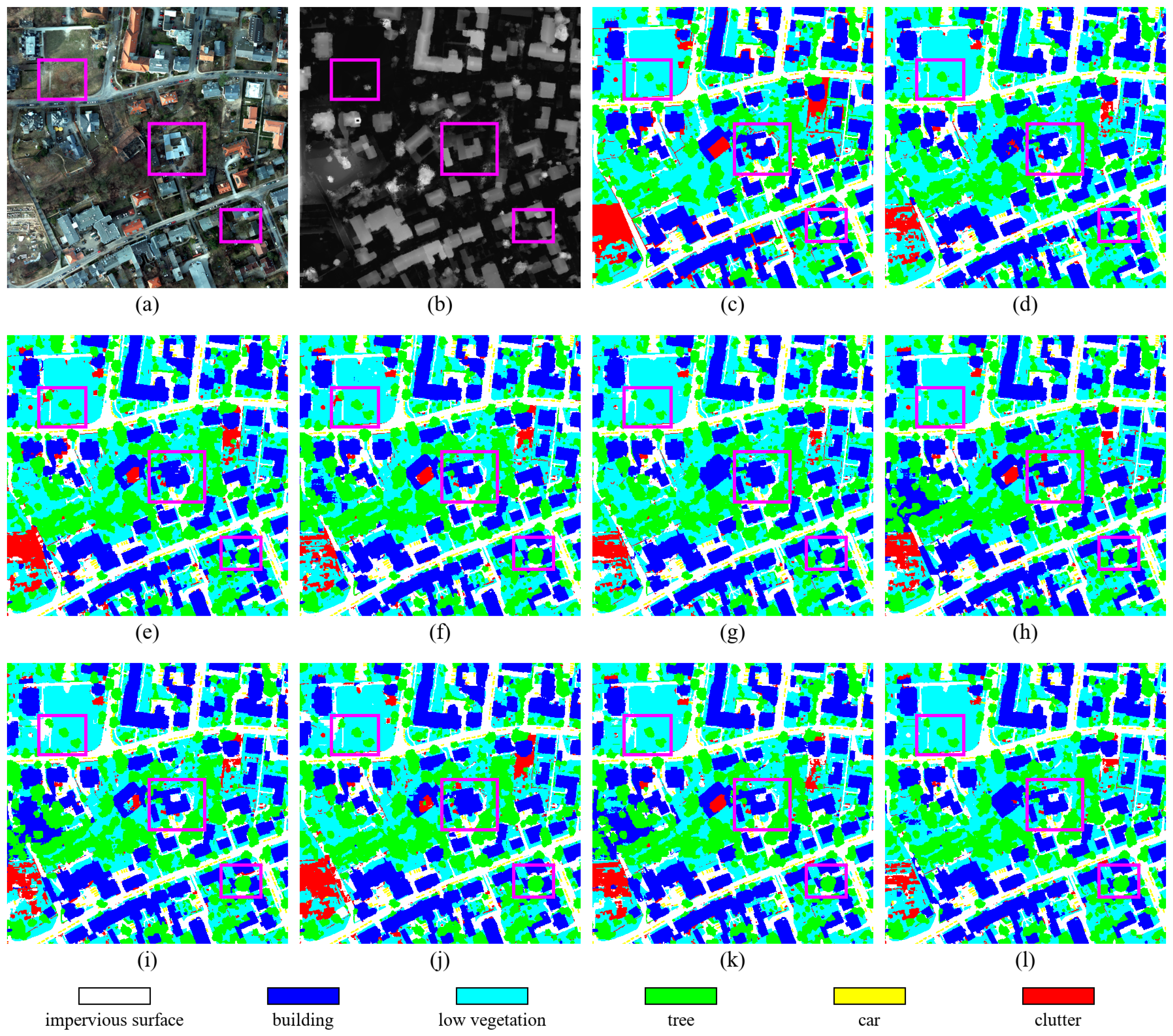
Figure 5 further illustrates the spatial prediction quality on the Potsdam dataset. The figure includes the optical image, nDSM, ground truth, predictions of representative methods, and the prediction of HDSMNet.

In the displayed Potsdam examples, HDSMNet produces comparatively coherent predictions around several building contours and adjacent impervious-surface regions, although local omissions and fine-boundary errors remain. This sample-level observation is consistent with the class-wise IoU results for buildings and impervious surfaces in Table 1, suggesting that height discontinuities and structural edges in nDSM may provide useful complementary information for spectrally similar regions. Several tree–low-vegetation transitions also appear locally less fragmented, while other ambiguous transitions remain difficult. For small objects such as cars, HDSMNet retains relatively clear responses in the selected road backgrounds. These localized behaviors may be associated with the geometry-guided fusion provided by HGSCF, while the adapted CGR path provides supplementary output refinement; they do not establish uniformly superior boundary quality across all categories and spatial scales.

In the middle highlighted region, tree shadows weaken the optical appearance of the building, and several optical-only baselines show local fragmentation or class confusion around the roof. The corresponding nDSM preserves a clear relative-height contrast, which may help HDSMNet maintain a comparatively coherent building response in this selected area under shadow occlusion.

The visual comparison also reveals several remaining failure cases. HDSMNet does not completely eliminate errors around narrow roof boundaries, thin road structures, and isolated small objects. These regions either occupy only a few pixels or exhibit weak local height contrast, limiting the geometric evidence available to HGSCF. In addition, local errors may remain when an nDSM boundary does not precisely coincide with the corresponding optical boundary. These observations suggest that height-derived guidance can support selected geometrically distinctive regions but cannot fully replace fine-grained appearance modeling and boundary-preserving mechanisms.

4.4.2. Comparison on the Vaihingen Dataset

Table 2 reports the comparison results on the Vaihingen dataset. Compared with Potsdam, Vaihingen contains fewer images, has a spatial resolution of 9 cm, and presents more compact spatial structures in the test areas. Therefore, this dataset can further evaluate the adaptability of HDSMNet under a smaller training scale and different spatial resolution.

In terms of overall metrics, HDSMNet achieves 92.06% OA, 91.18% mF1, and 84.22% mIoU on Vaihingen. It obtains the highest mF1 and mIoU among the compared methods, exceeding FTransUNet by 0.34 and 0.59 percentage points, respectively, although its OA is 0.20 percentage points lower. These results indicate that HDSMNet improves class-balanced segmentation quality without uniformly maximizing every metric.

The clearest class-level advantage appears for cars. HDSMNet achieves 86.76% IoU, outperforming the second-best RS3Mamba by 2.95 percentage points and FTransUNet by 4.97 percentage points. Cars occupy few pixels in the 9 cm Vaihingen imagery and are easily confused with roads, shadows, and surrounding impervious surfaces. Their local height discontinuities provide useful geometric evidence that may help HGSCF complement weak or ambiguous optical responses and retain small vehicle regions. This result supports an advantage for this small-object category but does not by itself indicate uniformly better boundary localization for other categories.

For buildings, trees, and impervious surfaces, HDSMNet obtains IoU values of 94.60%, 83.90%, and 87.57%, respectively. Although these values are not the highest, they are only 0.68, 0.24, and 0.23 percentage points below the corresponding best results, indicating competitive performance across major urban categories. Low vegetation remains a relative limitation: its IoU of 68.25% is below the best result of 69.12%. Unlike buildings, trees, or vehicles, low vegetation usually produces weak relative-height contrast with nearby ground surfaces, so nDSM contributes less distinctive geometric evidence. Its separation therefore depends more strongly on fine-grained spectral and textural cues, limiting the benefit available from height-guided fusion.

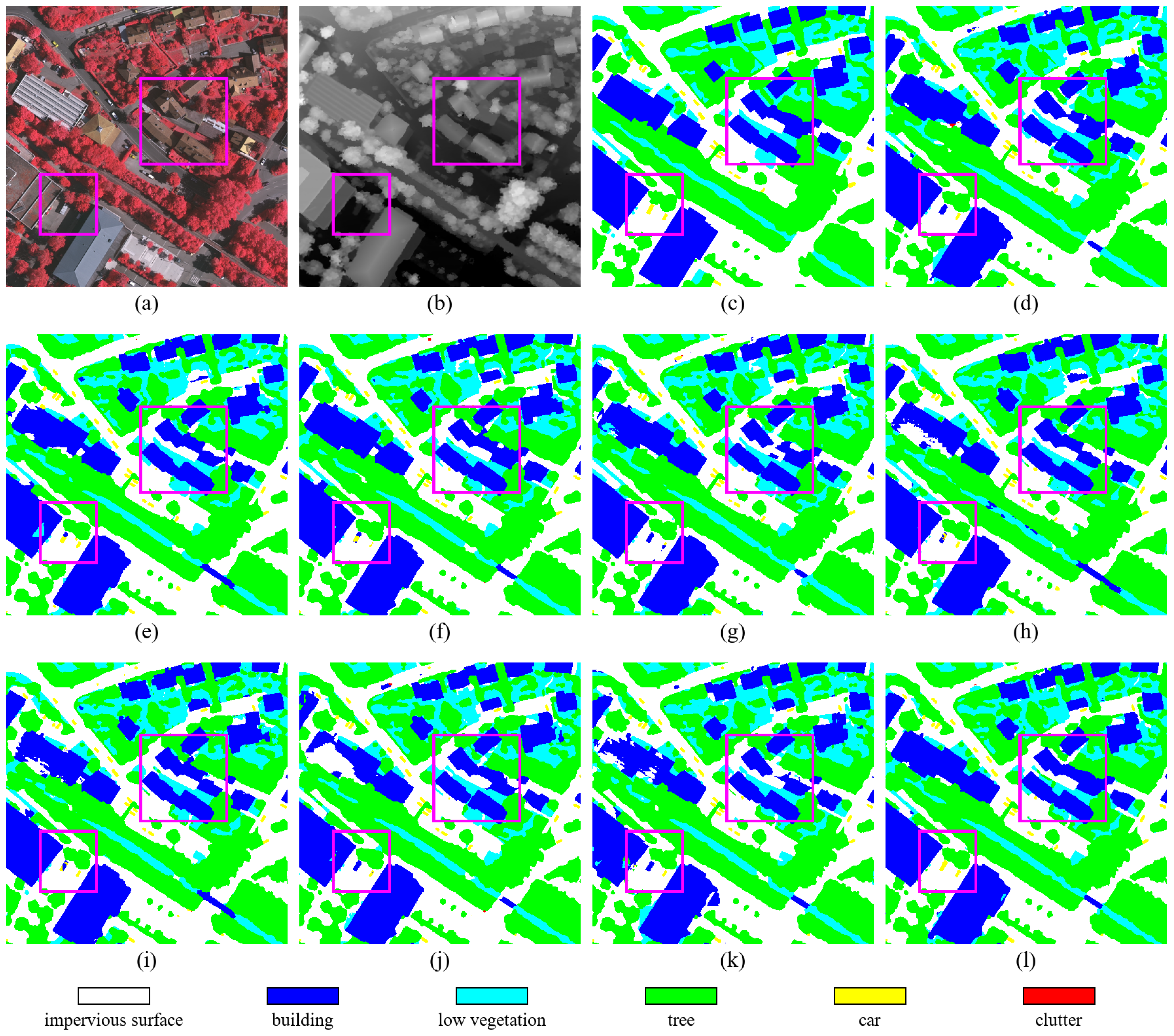
Figure 6 presents the visual comparison of prediction maps on the Vaihingen dataset. Compared with Potsdam, Vaihingen has lower spatial resolution, a smaller sample size, and more compact urban scenes. As a result, it is more prone to building boundary fragmentation, confusion between trees and low vegetation, and missed detection of small cars.

In the lower-left highlighted region, two cars lie in a heavily shadowed area of impervious surface. Several optical-only methods miss or confuse at least one car, whereas HDSMNet retains both car responses more clearly, suggesting that nDSM-derived height contrast and structural context can complement degraded optical appearance in shadowed regions.

In the highlighted examples, HDSMNet preserves several small vehicle regions comparatively well, which is consistent with its leading car IoU in Table 2. The method remains competitive around the displayed building and tree-canopy structures, although errors persist at some fine boundaries. By contrast, low-vegetation transitions remain difficult because these regions often lack strong relative-height contrast and must be distinguished mainly through optical appearance. Overall, the visual and quantitative results suggest that HDSMNet benefits most from objects with localized height discontinuities, while further improvement is needed for weak-height-signal categories and uncertain boundaries. This evidence is category- and region-dependent rather than an indication of uniformly superior boundary quality at every spatial scale.

5. Discussion

5.1. Ablation Study

The ablation study separates the effect of the proposed HGSCF module from that of the adapted output refinement path.

Table 3. Ablation study of the core modules and parameter counts on the Potsdam dataset. Checkmarks denote enabled components; bold values indicate the best result in each column.

HGSCF	CGR	Params (M)	OA (%)	mF1 (%)	mIoU (%)
–	–	52.116	90.66	91.62	84.85
–	✓	52.120	90.59	91.80	85.22
✓	–	64.906	91.23	92.29	86.00
✓	✓	64.910	91.54	92.63	86.57

and

Table 4. Ablation study of the core modules and parameter counts on the Vaihingen dataset. Checkmarks denote enabled components; bold values indicate the best result in each column.

HGSCF	CGR	Params (M)	OA (%)	mF1 (%)	mIoU (%)
–	–	52.114	91.52	90.07	82.26
–	✓	52.118	91.59	90.65	83.37
✓	–	64.904	92.12	91.02	83.93
✓	✓	64.908	92.06	91.18	84.22

report the results. The baseline keeps the same ConvNeXt V2 optical encoder, nDSM stem with VSSMEncoder, and UNet-style decoder as HDSMNet. When HGSCF is disabled, the fusion module is replaced by a static CatConvFusionBlock, which concatenates optical and nDSM features at each scale and projects them with a $1\times 1$ convolution. When CGR is disabled, the decoder uses the standard output path with the feature refinement layer and a $1\times 1$ classifier, without SpatialGatherModule or the DPG-style modulation module. HGSCF is evaluated as the principal fusion contribution, whereas CGR is evaluated to quantify the additional effect of supplementary classifier-conditioned output refinement.

On the Potsdam dataset, the baseline obtains 84.85% mIoU. Adding HGSCF alone increases the mIoU to 86.00%, a gain of 1.15 percentage points, whereas the adapted CGR component alone reaches 85.22%, a gain of 0.37 percentage points. Although CGR alone also increases mF1 from 91.62% to 91.80%, its OA decreases slightly from 90.66% to 90.59% ($-0.07$ percentage points). This comparison identifies height-guided fusion as the larger individual source of improvement, while classifier-conditioned refinement provides a smaller complementary gain in the class-balanced metrics without uniformly improving OA. When the two components are used together, the model achieves 91.54% OA, 92.63% mF1, and 86.57% mIoU, improving over the baseline by 0.88, 1.01, and 1.72 percentage points, respectively.

On the Vaihingen dataset, the mIoU improvements follow a similar pattern, but the metric-wise behavior is not uniform. HGSCF increases the mIoU from 82.26% to 83.93%, a gain of 1.67 percentage points, while the adapted CGR component alone reaches 83.37%, a gain of 1.11 percentage points. Adding CGR to HGSCF further increases mF1 from 91.02% to 91.18% and mIoU from 83.93% to 84.22%, but slightly reduces OA from 92.12% to 92.06% ($-0.06$ percentage points). Thus, CGR provides supplementary improvements in mF1 and mIoU, but its effect on OA is small and nonmonotonic.

The parameter counts further clarify the cost of each component. CGR adds only approximately 0.004 M parameters to the baseline on either dataset, whereas HGSCF adds approximately 12.790 M parameters and accounts for most of the additional model capacity. The full model contains 64.910 M parameters on Potsdam and 64.908 M on Vaihingen; the slight difference results from the four-channel and three-channel optical inputs, respectively. Thus, CGR provides complementary output refinement with negligible parameter growth, while the larger cost of HGSCF accompanies its stronger improvement in cross-modal feature fusion.

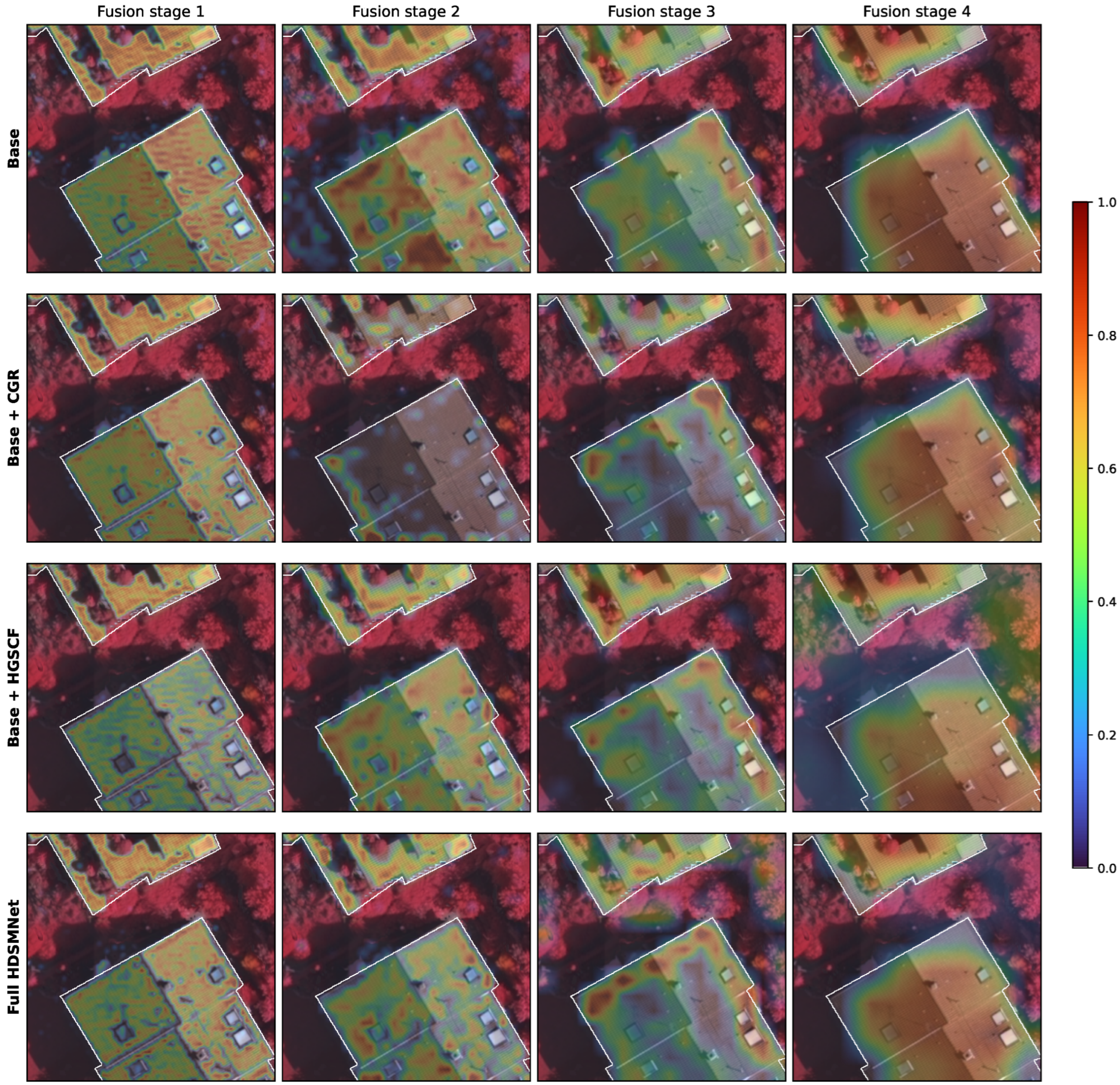
To further examine the effects of HGSCF and the adapted output refinement component, Figure 7 presents Grad-CAM visualizations for the building class at four fusion stages. The baseline produces relatively diffuse responses at the shallow and intermediate stages, with some activations extending into adjacent vegetation and shadowed regions. Adding the adapted CGR component alone mainly changes the deeper class-discriminative response, while its influence on early geometry localization remains limited. In contrast, the variants containing HGSCF generally show responses that are more closely aligned with building contours and roof regions at the early fusion stages. The full HDSMNet retains these geometry-aware responses and produces a more coherent building-focused activation at the final fusion stage. These observations are consistent with HGSCF serving as the primary geometry-aware fusion component and the adapted CGR component providing supplementary output refinement.

5.2. Hyperparameter Sensitivity Analysis

The HGSCF module contains two principal hyperparameters: the number of anchors K, which determines the size of the compact key/value interaction set, and the temperature coefficient $\tau$, which controls the sharpness of the spatial assignment distributions. Their sensitivity is evaluated on the Vaihingen dataset by varying one parameter at a time while keeping all other network structures and training settings unchanged.

Table 5. Sensitivity analysis of the anchor number K and temperature coefficient $\tau$ on the Vaihingen dataset. The difference is calculated relative to the default setting $K=16$ and $\tau =0.7$.

Sensitivity Factor	K	$\mathit{\tau }$	mIoU (%)	Difference (pp)
Anchor number	4	0.7	83.82	−0.40
Anchor number	16	0.7	84.22	0.00
Anchor number	32	0.7	83.92	−0.30
Temperature	16	0.3	83.63	−0.59
Temperature	16	0.7	84.22	0.00
Temperature	16	1.0	83.71	−0.51

summarizes the resulting mIoU values and their differences from the default setting.

With $\tau$ fixed at 0.7, increasing K from 4 to 16 improves the mIoU from 83.82% to 84.22%, whereas increasing it further to 32 reduces the mIoU to 83.92%. This suggests that too few anchors may be insufficient to represent diverse height structures and cross-modal discrepancies, while too many anchors may introduce redundant regional representations and weaken the compactness of sparse interaction.

With K fixed at 16, $\tau =0.7$ outperforms both 0.3 and 1.0. A lower temperature may produce overly concentrated spatial assignments, whereas a higher temperature may smooth the assignments and reduce their selectivity for discriminative geometric regions. The mIoU varies by at most 0.59 percentage points across all tested settings, indicating relatively stable performance over the evaluated ranges. Accordingly, $K=16$ and $\tau =0.7$ are adopted as the default configuration in the remaining experiments.

5.3. Model Complexity Analysis

To evaluate the resource consumption, inference efficiency, and segmentation performance of different methods, five indicators are used: the number of parameters (Params), floating-point operations (FLOPs), GPU memory consumption (memory), frames per second (FPS), and mIoU. Params reflects model size, FLOPs measure computational complexity, memory denotes inference memory consumption, and FPS measures patch-level inference throughput. An efficient semantic segmentation model should balance these resource costs and inference speed while maintaining reliable segmentation performance.

As shown in

Table 6. Computational complexity and inference-speed analysis measured with a batch size of 1 and a $256\times 256$ input on a single NVIDIA GeForce RTX 4090D GPU (NVIDIA Corporation, Santa Clara, CA, USA). The mIoU values are the results on the Vaihingen dataset, and bold values indicate the best results.

Method	Multimodal	Params (M)	FLOPs (G)	Memory (MB)	FPS	mIoU (%)
ABCNet	No	13.667	3.907	191.841	191.483	82.58
MAResU-Net	No	26.277	8.777	246.862	196.011	82.55
UNetFormer	No	11.725	2.935	184.921	176.354	80.12
RS3Mamba	No	43.325	15.825	326.756	82.882	82.55
ESANet	Yes	23.918	5.210	225.429	166.975	82.40
SA-Gate	Yes	110.850	41.287	597.909	91.115	78.15
FTransUNet	Yes	203.404	56.109	932.717	57.824	83.63
MCFMamba	Yes	63.429	13.346	561.387	32.835	80.90
MultiSenseSeg	Yes	58.656	66.069	398.179	54.361	81.18
HDSMNet	Yes	64.908	13.000	413.825	64.262	84.22

, single-modal models generally require fewer parameters, FLOPs, and memory. UNetFormer has the lowest values in these complexity indicators, but its mIoU is lower than that of HDSMNet. This is expected because single-modal models process only optical input and have shorter computational paths, but they lack nDSM height–structural information. Therefore, the complexity of HDSMNet should be interpreted together with its multimodal feature extraction objective, rather than only against lightweight single-modal models.

Among multimodal methods, HDSMNet shows a reasonable accuracy–complexity trade-off. Compared with FTransUNet, it reduces FLOPs, parameters, and memory consumption by approximately 76.8%, 68.1%, and 55.6%, respectively, while achieving a higher mIoU on Vaihingen. Compared with MCFMamba, HDSMNet has comparable FLOPs, lower memory consumption, and a 3.32 percentage-point improvement in mIoU. At the module level, the compact-anchor formulation limits query–context interaction to approximately $\mathcal{O}\left(N_{i}Kd\right)$, rather than the $\mathcal{O}\left(N_i^{2}d\right)$ pairwise interaction of dense global attention. The whole-model measurements in Table 6 indicate an accuracy–complexity trade-off under the evaluated configurations, but they are not used as a controlled comparison between HGSCF and alternative dense fusion blocks. The objective of HDSMNet is therefore not to minimize a single complexity indicator, but to obtain more discriminative dense features under controllable computational cost.

Under the same patch-level measurement setting, HDSMNet reaches 64.262 FPS, exceeding FTransUNet (57.824 FPS), MCFMamba (32.835 FPS), and MultiSenseSeg (54.361 FPS), although it remains slower than ESANet and SA-Gate. This result indicates that HDSMNet provides moderate inference throughput rather than an absolute speed advantage.

5.4. Error-Annotated Visualization Analysis

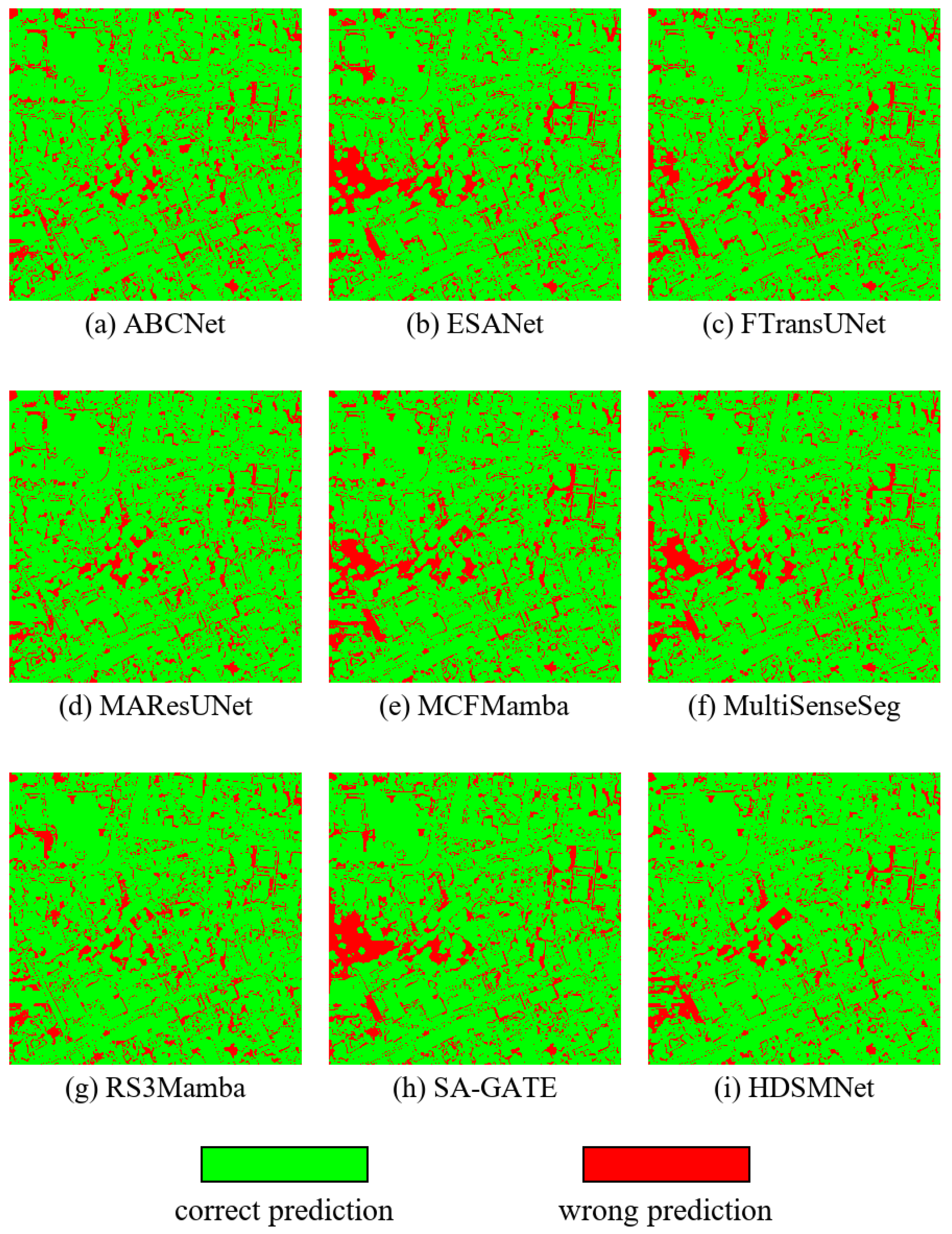
To further observe the spatial distribution of errors, binary error maps are drawn on the Potsdam dataset, as shown in Figure 8. Green indicates correctly classified pixels, while red indicates misclassified pixels. Compared with semantic prediction maps, error maps more directly reveal whether errors are concentrated around challenging segmentation regions, such as building boundaries, vegetation transitions, road structures, and small vehicle objects.

As shown in Figure 8, single-modal methods such as ABCNet and MAResU-Net produce scattered red error pixels around building boundaries, road networks, and vegetation regions with complex textures. This suggests that optical-only models are vulnerable to spectral similarity, shadows, and fragmented boundaries. Multimodal methods such as ESANet, SA-Gate, and MultiSenseSeg reduce errors in some regions, but continuous misclassifications remain around mixed building–road–vegetation areas and oblique linear structures, indicating that general fusion may not fully exploit discriminative geometric cues.

In the displayed example, HDSMNet exhibits fewer large continuous error regions, while the remaining errors are mainly located around complex boundaries, thin road structures, and small local objects. The associated predictions show fewer continuous errors in some spectrally similar regions, such as buildings versus impervious surfaces and trees versus low vegetation; however, this sample-level observation does not establish uniformly better boundary quality across all categories or spatial scales. The adapted component provides supplementary output refinement, whose measured contribution is reflected by the ablation gains in mF1 and mIoU. The remaining errors also show that HDSMNet does not fully eliminate fine boundary ambiguity, especially when height differences are weak, targets are extremely small, or annotation boundaries are uncertain.

5.5. Robustness to nDSM Corruptions

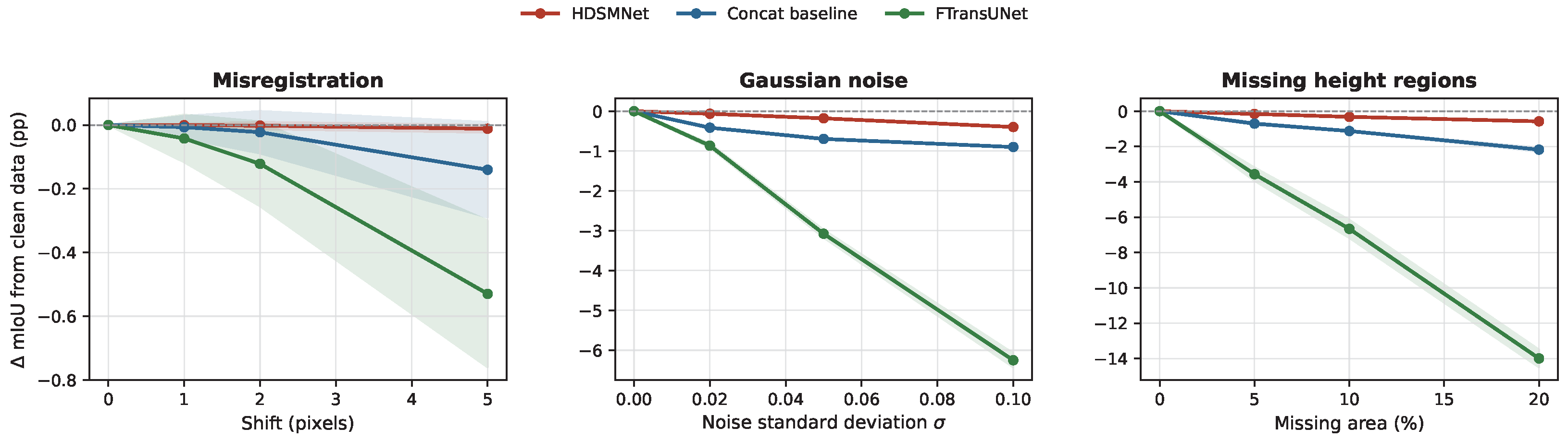
To quantify the influence of nDSM quality without changing the trained weights, controlled corruptions are applied only to the normalized nDSM input on the Vaihingen test set, while the optical input and inference settings remain unchanged. Three corruption types are considered: spatial shifts of 1, 2, and 5 pixels in four directions; additive Gaussian noise with $\sigma \in \{0.02,0.05,0.10\}$; and block-wise missing-height regions covering 5%, 10%, and 20% of the nDSM. The latter two settings are repeated with three random seeds. HDSMNet is compared with its static Concat fusion baseline using the same CGR output path and with FTransUNet. Figure 9 reports the complete degradation trends, and

Table 7. mIoU reduction under the highest tested severity of each nDSM corruption on the Vaihingen dataset. Positive values denote the magnitude of the reduction relative to the corresponding clean-input result.

Corruption Setting	HDSMNet Drop (pp)	Concat Baseline Drop (pp)	FTransUNet Drop (pp)
5-pixel spatial shift	0.01	0.14	0.53
Gaussian noise, $\sigma =0.10$	0.40	0.90	6.25
20% missing-height regions	0.58	2.18	14.00

Note: Bold values indicate the smallest mIoU reduction for each corruption setting.

summarizes the highest tested severity of each corruption.

Under a 5-pixel shift, all three methods show comparatively limited degradation, and HDSMNet has the smallest mean reduction. This suggests relatively low sensitivity to the tested spatial offsets, although the absolute difference from the Concat baseline remains modest. The separation becomes clearer under Gaussian noise: at $\sigma =0.10$, HDSMNet decreases by 0.40 percentage points, compared with 0.90 and 6.25 percentage points for the Concat baseline and FTransUNet, respectively. This result is consistent with selective geometry-guided interaction limiting the propagation of some local height perturbations, rather than treating every corrupted response as equally informative.

Missing-height regions provide the most discriminative setting among the evaluated corruptions. When 20% of the nDSM is removed, the mIoU reductions are 0.58, 2.18, and 14.00 percentage points for HDSMNet, the Concat baseline, and FTransUNet, respectively. The smaller degradation of HDSMNet suggests that its optical representation and sparse geometry-guided interaction retain useful complementary information when parts of the height input are unavailable. Nevertheless, performance continues to decrease as corruption severity increases, indicating that the robustness improvement is not complete and that stronger or compound data-quality disturbances may remain challenging.

5.6. Limitations

Although HDSMNet shows effectiveness in high-resolution urban remote sensing semantic segmentation, its applicability is still affected by cross-modal data quality and differences in object geometric structures.

First, HDSMNet remains dependent on the quality and spatial alignment of optical–nDSM data because HGSCF derives its guidance from the three encoded nDSM structural cues. The experiments in Section 5.5 show comparatively limited degradation within the evaluated corruption ranges; however, the performance still declines as the perturbation severity increases, indicating that sensitivity to registration quality and uncertain nDSM observations has not been fully eliminated. More severe misregistration, abnormal elevation values, and structured or compound nDSM artifacts may therefore still affect geometric guidance and sparse interaction. Future work should further improve adaptive reliability estimation for uncertain height observations.

Second, the class-wise results vary across datasets and categories. Some categories with relatively distinctive height structures obtain favorable results in individual settings, but the current evidence does not establish a consistent advantage across all categories or both datasets. For regions where height differences are weak and boundaries depend mainly on optical textures or local context, the model may still produce fine-grained misclassifications. This suggests that the nDSM geometric prior can complement the missing 3D structural information in optical imagery, but it cannot fully replace fine-grained spectral–textural modeling and boundary consistency constraints. For extremely small objects or thin structures, stronger boundary preservation and small-object enhancement strategies are still needed.

Third, the current controlled fusion comparison uses a static CatConv baseline under the same encoders and decoder. Dense cross-attention and SA-Gate-style gating have not been evaluated within this identical framework, and the context cue, local contrast, structural-discontinuity cue, and anchor geometry term inside HGSCF have not been separately ablated. Therefore, the present results support the aggregate benefit of the complete HGSCF module over CatConv, but do not establish superiority over all alternative fusion mechanisms or isolate the contribution of every internal cue. More comprehensive controlled comparisons and component-level ablations are left for future work.

Fourth, per-tile normalization of nDSM to $[0,1]$ improves input-scale stability but removes absolute height differences across tiles. Accordingly, the context cue used in this study should be interpreted as within-tile relative structural context rather than absolute elevation context. Comparing per-tile normalization with dataset-level global normalization is an important direction for evaluating whether cross-tile absolute height information provides additional benefit.

Finally, the implemented Context-Guided Refinement path uses a shared classifier and receives indirect supervision through the final segmentation loss. It has not been compared with direct auxiliary supervision, an independent coarse classifier, or other supervision strategies. Likewise, the asymmetric optical–height gating has not been evaluated against a symmetric gating variant under otherwise identical settings. The reported results therefore characterize the adopted design, but do not establish these choices as optimal; these alternatives warrant controlled evaluation in future work.

6. Conclusions

This study presents HDSMNet, a height-derived geometric-prior-guided framework for feature extraction and cross-modal fusion in high-resolution remote sensing semantic segmentation, with nDSM used as the elevation input in the experiments. HDSMNet adopts a dual-branch architecture to extract optical appearance features and nDSM height–structural features. Its main methodological component, HGSCF, performs selective interaction between the two modalities using the three nDSM-derived structural cues. An adapted Context-Guided Refinement (CGR) component provides supplementary classifier-conditioned output refinement after fusion.

HDSMNet achieves mIoU values of 86.57% and 84.22% on the ISPRS Potsdam and Vaihingen datasets, respectively. Ablation results show that HGSCF provides the larger individual improvement by strengthening height-guided cross-modal feature extraction, while the adapted output refinement component contributes smaller additional gains in mF1 and mIoU. Complexity analysis suggests that HDSMNet maintains a reasonable balance among accuracy, FLOPs, model parameters, and memory consumption, while the displayed visual examples show fewer continuous errors in some selected building, vegetation, and small-vehicle regions.

Future work will focus on improving robustness and efficiency. On the one hand, more robust geometric fusion mechanisms can be investigated to handle noisy nDSM data and cross-source registration errors, thereby improving the stability of the model under complex preprocessing conditions. On the other hand, the dual-branch encoder and HGSCF module can be further compressed to explore lightweight variants that are more suitable for edge devices and large-scale mapping tasks.

References

1. Wellmann, T.; Lausch, A.; Andersson, E.; Knapp, S.; Cortinovis, C.; Jache, J.; Scheuer, S.; Kremer, P.; Mascarenhas, A.; Kraemer, R.; et al. Remote sensing in urban planning: Contributions towards ecologically sound policies? Landsc. Urban Plan. 2020, 204, 103921. [Google Scholar] [CrossRef] [Scilit]
2. Weiss, M.; Jacob, F.; Duveiller, G. Remote sensing for agricultural applications: A meta-review. Remote Sens. Environ. 2020, 236, 111402. [Google Scholar] [CrossRef] [Scilit]
3. Yuan, X.; Shi, J.; Gu, L. A review of deep learning methods for semantic segmentation of remote sensing imagery. Expert Syst. Appl. 2021, 169, 114417. [Google Scholar] [CrossRef] [Scilit]
4. Diakogiannis, F.I.; Waldner, F.; Caccetta, P.; Wu, C. ResUNet-a: A Deep Learning Framework for Semantic Segmentation of Remotely Sensed Data. ISPRS J. Photogramm. Remote Sens. 2020, 162, 94–114. [Google Scholar] [CrossRef] [Scilit]
5. Wang, L.; Li, R.; Zhang, C.; Fang, S.; Duan, C.; Meng, X.; Atkinson, P.M. UNetFormer: A UNet-like Transformer for Efficient Semantic Segmentation of Remote Sensing Urban Scene Imagery. ISPRS J. Photogramm. Remote Sens. 2022, 190, 196–214. [Google Scholar] [CrossRef] [Scilit]
6. Long, J.; Shelhamer, E.; Darrell, T. Fully Convolutional Networks for Semantic Segmentation. In Proceedings of the IEEE Conference on Computer Vision and Pattern Recognition (CVPR), Boston, MA, USA, 7–12 June 2015; pp. 3431–3440. [Google Scholar] [CrossRef] [Scilit]
7. Ronneberger, O.; Fischer, P.; Brox, T. U-Net: Convolutional Networks for Biomedical Image Segmentation. In Medical Image Computing and Computer-Assisted Intervention–MICCAI 2015; Springer: Cham, Switzerland, 2015; pp. 234–241. [Google Scholar] [CrossRef] [Scilit]
8. Chen, L.-C.; Zhu, Y.; Papandreou, G.; Schroff, F.; Adam, H. Encoder–Decoder with Atrous Separable Convolution for Semantic Image Segmentation. In Computer Vision–ECCV 2018; Springer: Cham, Switzerland, 2018; pp. 833–851. [Google Scholar] [CrossRef] [Scilit]
9. Zhao, H.; Shi, J.; Qi, X.; Wang, X.; Jia, J. Pyramid Scene Parsing Network. In Proceedings of the IEEE Conference on Computer Vision and Pattern Recognition (CVPR), Honolulu, HI, USA, 21–26 July 2017; pp. 2881–2890. [Google Scholar] [CrossRef] [Scilit]
10. Dosovitskiy, A.; Beyer, L.; Kolesnikov, A.; Weissenborn, D.; Zhai, X.; Unterthiner, T.; Dehghani, M.; Minderer, M.; Heigold, G.; Gelly, S.; et al. An Image Is Worth 16×16 Words: Transformers for Image Recognition at Scale. In Proceedings of the International Conference on Learning Representations (ICLR), Virtual Event, 3–7 May 2021; Available online: https://openreview.net/forum?id=YicbFdNTTy (accessed on 15 August 2026).
11. Liu, Z.; Lin, Y.; Cao, Y.; Hu, H.; Wei, Y.; Zhang, Z.; Lin, S.; Guo, B. Swin Transformer: Hierarchical Vision Transformer Using Shifted Windows. In Proceedings of the IEEE/CVF International Conference on Computer Vision (ICCV), Montreal, BC, Canada, 10–17 October 2021; pp. 10012–10022. [Google Scholar] [CrossRef] [Scilit]
12. Gu, A.; Dao, T. Mamba: Linear-Time Sequence Modeling with Selective State Spaces. arXiv 2023, arXiv:2312.00752. [Google Scholar] [CrossRef] [Scilit]
13. Liu, Y.; Tian, Y.; Zhao, Y.; Yu, H.; Xie, L.; Wang, Y.; Ye, Q.; Jiao, J.; Liu, Y. VMamba: Visual State Space Model. In Advances in Neural Information Processing Systems; Curran Associates: Red Hook, NY, USA, 2024; Volume 37. [Google Scholar] [CrossRef] [Scilit]
14. Hazirbas, C.; Ma, L.; Domokos, C.; Cremers, D. FuseNet: Incorporating Depth into Semantic Segmentation via Fusion-Based CNN Architecture. In Computer Vision–ACCV 2016 Workshops; Springer: Cham, Switzerland, 2017; pp. 213–228. [Google Scholar] [CrossRef] [Scilit]
15. Ma, X.; Zhang, X.; Pun, M.-O. A Crossmodal Multiscale Fusion Network for Semantic Segmentation of Remote Sensing Data. IEEE J. Sel. Top. Appl. Earth Obs. Remote Sens. 2022, 15, 3463–3474. [Google Scholar] [CrossRef] [Scilit]
16. Ma, X.; Zhang, X.; Pun, M.-O.; Liu, M. A Multilevel Multimodal Fusion Transformer for Remote Sensing Semantic Segmentation. IEEE Trans. Geosci. Remote Sens. 2024, 62, 5403215. [Google Scholar] [CrossRef] [Scilit]
17. Feng, H.; Hu, Q.; Zhao, P.; Wang, S.; Ai, M.; Zheng, D.; Liu, T. FTransDeepLab: Multimodal Fusion Transformer-Based DeepLabv3+ for Remote Sensing Semantic Segmentation. IEEE Trans. Geosci. Remote Sens. 2025, 63, 4406618. [Google Scholar] [CrossRef] [Scilit]
18. Wang, Z.; Li, J.; Xu, N.; You, Z. Combining Feature Compensation and GCN-Based Reconstruction for Multimodal Remote Sensing Image Semantic Segmentation. Inf. Fusion 2025, 122, 103207. [Google Scholar] [CrossRef] [Scilit]
19. Zhao, Y.; Qiu, L.; Yang, Z.; Chen, Y.; Zhang, Y. MGF-GCN: Multimodal Interaction Mamba-Aided Graph Convolutional Fusion Network for Semantic Segmentation of Remote Sensing Images. Inf. Fusion 2025, 122, 103150. [Google Scholar] [CrossRef] [Scilit]
20. Wang, Y.; Cao, L.; Deng, H. MFMamba: A Mamba-Based Multi-Modal Fusion Network for Semantic Segmentation of Remote Sensing Images. Sensors 2024, 24, 7266. [Google Scholar] [CrossRef] [Scilit]
21. Qiu, J.; Chang, W.; Ren, W.; Hou, S.; Yang, R. MMFNet: A Mamba-Based Multimodal Fusion Network for Remote Sensing Image Semantic Segmentation. Sensors 2025, 25, 6225. [Google Scholar] [CrossRef] [Scilit]
22. Li, C.; Lyu, H.; Jing, W.; Yuan, Y.; Cheng, G. MFFNet: A Wavelet Transform-Based Multimodal Frequency Fusion Network for Remote Sensing Semantic Segmentation. GISci. Remote Sens. 2025, 62, 2534740. [Google Scholar] [CrossRef] [Scilit]
23. Cai, J.; Su, J.; Li, Q.; Yang, W.; Wang, S.; Zhao, T.; He, S.; Liu, W. Keep the Balance: A Parameter-Efficient Symmetrical Framework for RGB+X Semantic Segmentation. In Proceedings of the IEEE/CVF Conference on Computer Vision and Pattern Recognition (CVPR), Nashville, TN, USA, 11–15 June 2025; pp. 10587–10598. [Google Scholar] [CrossRef] [Scilit]
24. Du, S.; Wang, W.; Guo, R.; Wang, R.; Tang, S. AsymFormer: Asymmetrical Cross-Modal Representation Learning for Mobile Platform Real-Time RGB-D Semantic Segmentation. In Proceedings of the IEEE/CVF Conference on Computer Vision and Pattern Recognition Workshops (CVPRW), Seattle, WA, USA, 17–21 June 2024; pp. 7608–7615. [Google Scholar] [CrossRef] [Scilit]
25. Yuan, Y.; Chen, X.; Wang, J. Object-Contextual Representations for Semantic Segmentation. In Computer Vision–ECCV 2020; Springer: Cham, Switzerland, 2020; pp. 173–190. [Google Scholar] [CrossRef] [Scilit]
26. Ni, Z.; Chen, X.; Zhai, Y.; Tang, Y.; Wang, Y. Context-Guided Spatial Feature Reconstruction for Efficient Semantic Segmentation. In Computer Vision–ECCV 2024; Lecture Notes in Computer Science; Springer: Cham, Switzerland, 2025; Volume 15110, pp. 239–255. [Google Scholar] [CrossRef] [Scilit]
27. Woo, S.; Debnath, S.; Hu, R.; Chen, X.; Liu, Z.; Kweon, I.S.; Xie, S. ConvNeXt V2: Co-Designing and Scaling ConvNets with Masked Autoencoders. In Proceedings of the IEEE/CVF Conference on Computer Vision and Pattern Recognition (CVPR), Vancouver, BC, Canada, 18–22 June 2023; pp. 16133–16142. [Google Scholar] [CrossRef] [Scilit]
28. Zheng, S.; Lu, J.; Zhao, H.; Zhu, X.; Luo, Z.; Wang, Y.; Fu, Y.; Feng, J.; Xiang, T.; Torr, P.H.S.; et al. Rethinking Semantic Segmentation from a Sequence-to-Sequence Perspective with Transformers. In Proceedings of the IEEE/CVF Conference on Computer Vision and Pattern Recognition (CVPR), Virtual Event, 19–25 June 2021; pp. 6881–6890. [Google Scholar] [CrossRef] [Scilit]
29. Xie, E.; Wang, W.; Yu, Z.; Anandkumar, A.; Alvarez, J.M.; Luo, P. SegFormer: Simple and Efficient Design for Semantic Segmentation with Transformers. In Advances in Neural Information Processing Systems; Curran Associates: Red Hook, NY, USA, 2021; Volume 34, pp. 12077–12090. Available online: https://proceedings.neurips.cc/paper_files/paper/2021/hash/64f1f27bf1b4ec22924fd0acb550c235-Abstract.html (accessed on 27 August 2026).
30. Audebert, N.; Le Saux, B.; Lefèvre, S. Beyond RGB: Very High Resolution Urban Remote Sensing with Multimodal Deep Networks. ISPRS J. Photogramm. Remote Sens. 2018, 140, 20–32. [Google Scholar] [CrossRef] [Scilit]
31. Hosseinpour, H.; Samadzadegan, F.; Dadrass Javan, F. CMGFNet: A Deep Cross-Modal Gated Fusion Network for Building Extraction from Very High-Resolution Remote Sensing Images. ISPRS J. Photogramm. Remote Sens. 2022, 184, 96–115. [Google Scholar] [CrossRef] [Scilit]
32. Zheng, X.; Wu, X.; Huan, L.; He, W.; Zhang, H. A Gather-to-Guide Network for Remote Sensing Semantic Segmentation of RGB and Auxiliary Image. IEEE Trans. Geosci. Remote Sens. 2022, 60, 5404915. [Google Scholar] [CrossRef] [Scilit]
33. Zhou, W.; Jin, J.; Lei, J.; Yu, L. CIMFNet: Cross-Layer Interaction and Multiscale Fusion Network for Semantic Segmentation of High-Resolution Remote Sensing Images. IEEE J. Sel. Top. Signal Process. 2022, 16, 666–676. [Google Scholar] [CrossRef] [Scilit]
34. Fan, X.; Zhou, W.; Qian, X.; Yan, W. Progressive Adjacent-Layer Coordination Symmetric Cascade Network for Semantic Segmentation of Multimodal Remote Sensing Images. Expert Syst. Appl. 2024, 238, 121999. [Google Scholar] [CrossRef] [Scilit]
35. Huang, X.; Zhang, X.; Wang, L.; Yuan, D.; Xu, S.; Zhou, F.; Zhou, Z. MMA-Net: A Semantic Segmentation Network for High-Resolution Remote Sensing Images Based on Multimodal Fusion and Multi-Scale Multi-Attention Mechanisms. Remote Sens. 2025, 17, 3572. [Google Scholar] [CrossRef] [Scilit]
36. Gu, A.; Goel, K.; Ré, C. Efficiently Modeling Long Sequences with Structured State Spaces. In Proceedings of the International Conference on Learning Representations (ICLR), Virtual Event, 25–29 April 2022. [Google Scholar] [CrossRef] [Scilit]
37. Zhu, L.; Liao, B.; Zhang, Q.; Wang, X.; Liu, W.; Wang, X. Vision Mamba: Efficient Visual Representation Learning with Bidirectional State Space Model. In Proceedings of the 41st International Conference on Machine Learning; Proceedings of Machine Learning Research; PMLR: Cambridge, MA, USA, 2024; Volume 235, pp. 62429–62442. Available online: https://proceedings.mlr.press/v235/zhu24f.html (accessed on 27 August 2026).
38. Ma, X.; Zhang, X.; Pun, M.-O. RS3Mamba: Visual State Space Model for Remote Sensing Image Semantic Segmentation. IEEE Geosci. Remote Sens. Lett. 2024, 21, 6011405. [Google Scholar] [CrossRef] [Scilit]
39. Chen, H.; Luo, H.; Wang, C. AfaMamba: Adaptive Feature Aggregation with Visual State Space Model for Remote Sensing Images Semantic Segmentation. IEEE J. Sel. Top. Appl. Earth Obs. Remote Sens. 2025, 18, 8965–8983. [Google Scholar] [CrossRef] [Scilit]
40. Jin, J.; Zhou, W.; Yang, R.; Ye, L.; Yu, L. Edge Detection Guide Network for Semantic Segmentation of Remote-Sensing Images. IEEE Geosci. Remote Sens. Lett. 2023, 20, 5000505. [Google Scholar] [CrossRef] [Scilit]
41. Li, R.; Zheng, S.; Zhang, C.; Duan, C.; Wang, L.; Atkinson, P.M. ABCNet: Attentive Bilateral Contextual Network for Efficient Semantic Segmentation of Fine-Resolution Remotely Sensed Imagery. ISPRS J. Photogramm. Remote Sens. 2021, 181, 84–98. [Google Scholar] [CrossRef] [Scilit]
42. Li, R.; Zheng, S.; Duan, C.; Su, J.; Zhang, C. Multistage Attention ResU-Net for Semantic Segmentation of Fine-Resolution Remote Sensing Images. IEEE Geosci. Remote Sens. Lett. 2022, 19, 8009205. [Google Scholar] [CrossRef] [Scilit]
43. Seichter, D.; Köhler, M.; Lewandowski, B.; Wengefeld, T.; Gross, H.-M. Efficient RGB-D Semantic Segmentation for Indoor Scene Analysis. In Proceedings of the IEEE International Conference on Robotics and Automation (ICRA), Xi’an, China, 30 May–5 June 2021; pp. 13525–13531. [Google Scholar] [CrossRef] [Scilit]
44. Chen, X.; Lin, K.-Y.; Wang, J.; Wu, W.; Qian, C.; Li, H.; Zeng, G. Bi-Directional Cross-Modality Feature Propagation with Separation-and-Aggregation Gate for RGB-D Semantic Segmentation. In Computer Vision–ECCV 2020; Springer: Cham, Switzerland, 2020; pp. 561–577. [Google Scholar] [CrossRef] [Scilit]
45. Liu, X.; Wang, T.; Jin, F.; Rui, J.; Wang, S.; Huang, Z.; Zou, Y.; Yu, X. Multimodal Cross Fusion Mamba Network for Remote Sensing Image Semantic Segmentation with Complementary Masked Self-Supervision. Int. J. Appl. Earth Obs. Geoinf. 2025, 145, 104960. [Google Scholar] [CrossRef] [Scilit]
46. Wang, Q.; Chen, W.; Huang, Z.; Tang, H.; Yang, L. MultiSenseSeg: A Cost-Effective Unified Multimodal Semantic Segmentation Model for Remote Sensing. IEEE Trans. Geosci. Remote Sens. 2024, 62, 4703724. [Google Scholar] [CrossRef] [Scilit]
Figure 1. Examples highlighting the characteristics of high-resolution remote sensing images, drawn from the ISPRS Potsdam dataset. (a) First representative optical–nDSM sample pair; (b) second representative optical–nDSM sample pair; (c) third representative optical–nDSM sample pair. In each pair, the upper image is the optical image and the lower image is the corresponding nDSM.
Remotesensing 18 02992 g001
Figure 2. Overall architecture of HDSMNet. The network extracts multiscale optical and nDSM features, fuses them with HGSCF blocks, and generates the final segmentation map through a skip-connected decoder with an adapted Context-Guided Refinement (CGR) path.
Remotesensing 18 02992 g002
Figure 3. Structure of the HGSCF module. The module takes optical and nDSM branch features as inputs, derives three complementary structural cues in the encoded feature space, and performs cross-modal fusion through geometry-aware gating and sparse anchor-based cross-attention.
Remotesensing 18 02992 g003
Figure 4. Adapted Context-Guided Refinement (CGR). An intermediate class-indexed response generated by the shared classifier guides contextual aggregation, followed by DPG-style dynamic modulation of the decoder features.
Remotesensing 18 02992 g004
Figure 5. Visual comparison on the Potsdam dataset. (a) Optical image, (b) nDSM, (c) ground truth, (d) ABCNet, (e) UNetFormer, (f) FTransUNet, (g) MAResU-Net, (h) MCFMamba, (i) MultiSenseSeg, (j) RS3Mamba, (k) SA-Gate, and (l) HDSMNet. The magenta boxes highlight representative regions with visually noticeable differences.
Remotesensing 18 02992 g005
Figure 6. Visual comparison on the Vaihingen dataset. (a) Optical image, (b) nDSM, (c) ground truth, (d) ABCNet, (e) ESANet, (f) FTransUNet, (g) MAResU-Net, (h) MCFMamba, (i) MultiSenseSeg, (j) RS3Mamba, (k) UNetFormer, and (l) HDSMNet. The magenta boxes highlight representative regions with visually noticeable differences.
Remotesensing 18 02992 g006
Figure 7. Grad-CAM comparison for the building class. Columns from left to right show fusion stages 1–4, and rows from top to bottom show the Base, Base + CGR, Base + HGSCF, and full HDSMNet variants.
Remotesensing 18 02992 g007
Figure 8. Binary error maps of different methods on the Potsdam dataset. Green indicates correctly classified pixels, while red indicates misclassified pixels. (a) ABCNet, (b) ESANet, (c) FTransUNet, (d) MAResU-Net, (e) MCFMamba, (f) MultiSenseSeg, (g) RS3Mamba, (h) SA-Gate, and (i) HDSMNet.
Remotesensing 18 02992 g008
Figure 9. Clean-relative mIoU degradation under controlled nDSM corruptions on the Vaihingen dataset: (a) misregistration; (b) Gaussian noise; and (c) missing-height regions. Spatial shifts are averaged over four directions, whereas Gaussian noise and missing-height regions are averaged over three random seeds; shaded regions indicate the corresponding standard deviations.
Remotesensing 18 02992 g009