1. Introduction
Soil moisture (SM) is an important state variable in the terrestrial water cycle and plays a critical role in land–atmosphere interactions [
1,
2]. Due to the strong spatiotemporal variability of SM, traditional point-based monitoring techniques struggle to capture its spatial patterns across extensive regions over long time series [
3,
4]. Remote sensing, depending on its special observation ability at a large scale, has shown remarkable advantages for SM mapping [
2]. Observations from both microwave and optical remote sensing have been widely used to obtain SM information across broad spatial and temporal extents [
5]. However, the global and regional SM products retrieved from current satellite remote sensors generally have coarse spatial resolutions [
6], which restricts their applications at fine spatial domains. For this reason, generating high-resolution SM datasets has emerged as a prominent yet challenging research focus within this discipline.
To meet the increasing demand for high-resolution SM data, numerous algorithms have been developed by relevant researchers to fulfill this demand [
7]. One mainstream approach directly retrieves fine-resolution SM from high-spatial-resolution satellite measurements with radiative transfer models. Fan et al. [
8] derived global 1 km SM products from Sentinel-1 observations using a semi-empirical water cloud model. This method requires relatively few auxiliary datasets, but its accuracy heavily relies on well-calibrated radiative transfer models with robust simulation performance. Spatial downscaling represents another effective strategy for generating fine-resolution SM products [
4]. This technique is built on the surface correlation between coarse- and fine-resolution remote sensing retrievals. Researchers establish scale transformation functions for SM using visible bands, thermal infrared signals, or vegetation-related auxiliary variables, which compensate for the spatial detail loss inherent to coarse microwave observations [
9,
10,
11,
12]. The core principle lies in mitigating surface heterogeneity errors caused by scale discrepancies through covariates such as vegetation and land surface temperature, thereby refining coarse-resolution SM products into high-spatial-resolution datasets. Based on the thermal inertia theory, Fang et al. [
9] constructed an SM downscaling framework to disaggregate the 9 km SMAP enhanced L2 radiometer SM product down to 1 km. Using machine learning methods, Zheng et al. [
10] downscaled CCI SM data to a 1 km grid by integrating International Soil Moisture Network (ISMN) ground measurements and high-resolution optical imagery. The third category employs machine learning or deep learning approaches [
1] to directly integrate multi-source high-resolution satellite observations or auxiliary datasets to retrieve 1 km SM [
2,
5]. Adopting a random forest model, Han et al. [
13] generated daily global topsoil SM at 1 km resolution by combining meteorological forcing data, static soil physical parameters, and multi-source optical remote sensing records. Following a comparable modeling strategy, Li et al. [
14] produced daily 1 km SM products with inputs including ERA5-Land reanalysis, leaf area index (LAI), land cover, digital elevation model (DEM) and soil property datasets. Using the XGBoost framework, Zhang et al. [
15] constructed a spatiotemporally continuous, global daily dataset at 1 km resolution by merging GLASS products, ERA5-Land reanalysis datasets, environmental auxiliary datasets, and in situ SM observations from ISMN. All three of the above strategies are extensively adopted to produce the fine-resolution SM datasets for regional and global research applications.
Nearly all the SM retrieval methods outlined above integrate multi-source datasets as model inputs [
16,
17,
18]. Such input variables fall into two distinct categories based on temporal characteristics: dynamic predictors and static predictors. Dynamic predictors include high-resolution visible, thermal infrared and active microwave remote sensing imagery, resampled atmospheric reanalysis products, and other auxiliary datasets. Static predictors consist of geographic coordinates, topographic metrics, land cover, and inherent soil attributes. Sentinel-1, Sentinel-2, and MODIS retrievals serve as primary high-resolution data sources, which can capture fine domain spatial variations in land surface conditions. ERA5 or ERA5-Land reanalysis datasets are widely incorporated as background meteorological inputs, supplying variables such as surface SM, land surface temperature, and precipitation. Coarse-resolution SM products are also occasionally incorporated into model frameworks. Furthermore, soil texture metrics (e.g., sand fraction, clay fraction) and bulk density are standard proxies to characterize soil physical properties. Collectively, these predictive covariates have become standard inputs for regional and global SM estimation. Nevertheless, the relative contribution of each individual predictor to the final SM retrieval outputs has not yet been systematically quantified.
Three mainstream frameworks exist to quantify the relative influence of input predictors [
19]: built-in feature importance from tree-based ensembles, model-agnostic interpretability techniques (e.g., permutation importance, SHAP), and conventional statistical decomposition approaches. Tree-based models including random forest, XGBoost, LightGBM and CatBoost natively support feature importance scoring [
20,
21,
22]. Random forest supplies two standard metrics, namely, Gini feature importance and permutation importance, rendering it the most prevalent tool for SM retrieval studies in remote sensing [
20]. Gradient boosting frameworks such as XGBoost output gain-based importance scores, which can quantify the total contribution ratio of each predictor to SM fitting [
21]. A key strength of all tree-based ensemble methods is their computational efficiency. They produce importance rankings directly after training without the need for auxiliary models and minimal extra computation. Model-agnostic global interpretability techniques form a second group, which are compatible with any machine learning or deep learning architecture. For instance, the permutation importance approach disrupts the values of a single variable and measures the resulting decline in model accuracy [
23]. A larger accuracy drop indicates a higher contribution of that predictor, offering an intuitive physical interpretation. Based on game theory, SHAP quantifies positive and negative contributions for each individual sample [
24]. It generates a global average importance ranking and differentiates linear versus nonlinear predictor responses, establishing it as the leading interpretability method within contemporary SM downscaling literature. Local interpretability models focus on local contributions at individual pixels, and are suitable for analyzing typical sampling points in small study areas, yet they perform less effectively than SHAP in global contribution assessment. Finally, classical statistical decomposition workflows can be paired with machine learning outputs. Variance decomposition and hierarchical partitioning (H-statistic) separately quantify each variable’s independent and interactive effects [
25]. Partial dependence plots (PDP) and individual conditional expectation (ICE) curves visualize how model outputs shift alongside changing predictor values [
22,
26], offering indirect insights into variable influence. Standardized multiple linear regression coefficients serve only linear modeling contexts, where absolute coefficient magnitudes signal variable importance. However, this approach yields significant bias when applied to nonlinear datasets. Across all interpretability tools outlined above, SHAP remains the dominant choice within SM retrieval research for the comparative analysis of multi-source covariate weights.
Most existing machine learning-based SM retrieval studies adopt a fixed spatial resolution, ignoring how spatial differences modulate the contribution of model predictors. To address this gap, this work couples an XGBoost regression with the SHAP interpretability framework. Two modeling schemes are established, namely, independent site-specific models and a unified global model. Ultimately, this study aims to quantitatively reveal how the contribution magnitudes and driving mechanism of input predictors (including vegetation, radar, topography, and meteorological variables) for SM retrieval evolve across a varying spatial domain.
4. Results
4.1. Performance Assessment of SM Retrievals
Table 3 summarizes the statistical metrics (Bias, RMSE and R
2) of the XGBoost models trained separately on eight independent monitoring networks and the combined global networks, with performance reported for both training and validation datasets. The XGBoost model demonstrates a strong capability in capturing the nonlinear relationships between input features and SM, as evidenced by the consistently high training and validation accuracies across all networks. The near-zero biases for both training and validation datasets further indicate the absence of systematic overestimation or underestimation, which provides a statistically unbiased residual background for the subsequent SHAP-based interpretability analysis. However, a pronounced performance gap exists between training and validation datasets across all networks, with validation R
2 values falling within a considerably wider range of 0.764–0.945. This broad variance in validation datasets is theoretically expected, and is hypothesized to reflect the underlying spatial heterogeneity of each monitoring network. The REMEDHUS network achieves the optimal validation performance, followed by FMI, COSMOS-UK, and SMOSMANIA-SWATMEX. These four networks yield validation R
2 values exceeding 0.900, demonstrating that the XGBoost model can effectively capture dominant SM controls within their respective local domains. In contrast, the SNOTEL network exhibits the weakest generalization ability among all independent datasets, recording the highest validation RMSE and the lowest R
2. Moderate retrieval accuracy is recorded for SCAN, USCRN, and RSMN. Even though the XGBoost model at the RSMN network shows near perfect training performance, its validation R
2 drops to 0.894, implying substantial overfitting within this local network.
For each individual network, the XGBoost model achieves exceptionally high training accuracy but consistently degraded validation accuracy. Interestingly, when all networks are aggregated into a single training set (the ISMN SM dataset in the last row), the model exhibits fundamentally different behavior. The training accuracy (R2 = 0.865) is considerably lower than that of any individual network, which is expected given the substantially increased feature space complexity and the inclusion of diverse, sometimes conflicting, land surface signatures. Although the global merged model yields a lower training set R2 (0.865) than any individual regional-domain model, it exhibits a comparatively smaller degradation from training to validation performance. This pattern indicates the reduced risk of over-fitting to site-specific local land surface signatures and better cross-domain stability across heterogeneous conditions, rather than superior absolute prediction accuracy. Indeed, seven of eight regional-domain models achieve higher validation set R2 values within their respective local domains.
To complement the quantitative statistical metrics presented in
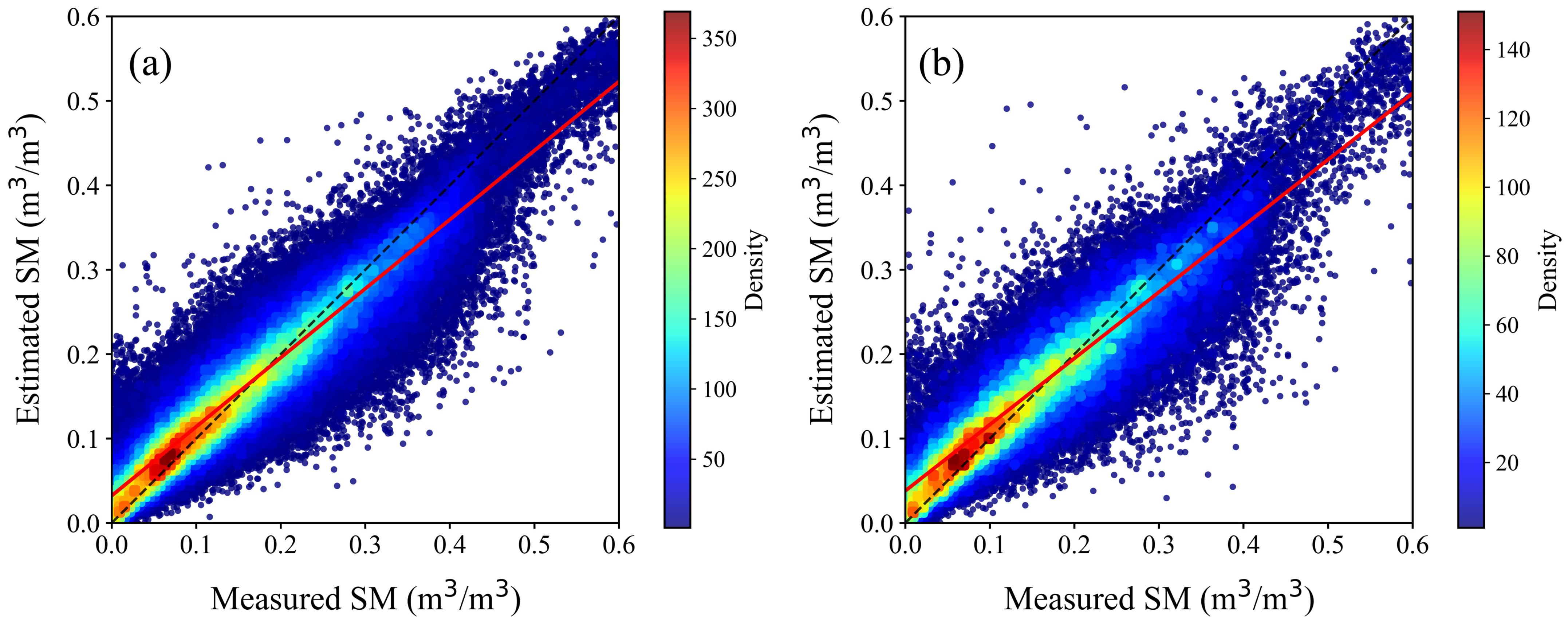
Table 3, density-colored scatterplots illustrate the consistency between the estimated and measured SM across the global merged ISMN datasets (
Figure 2) and individual monitoring networks (
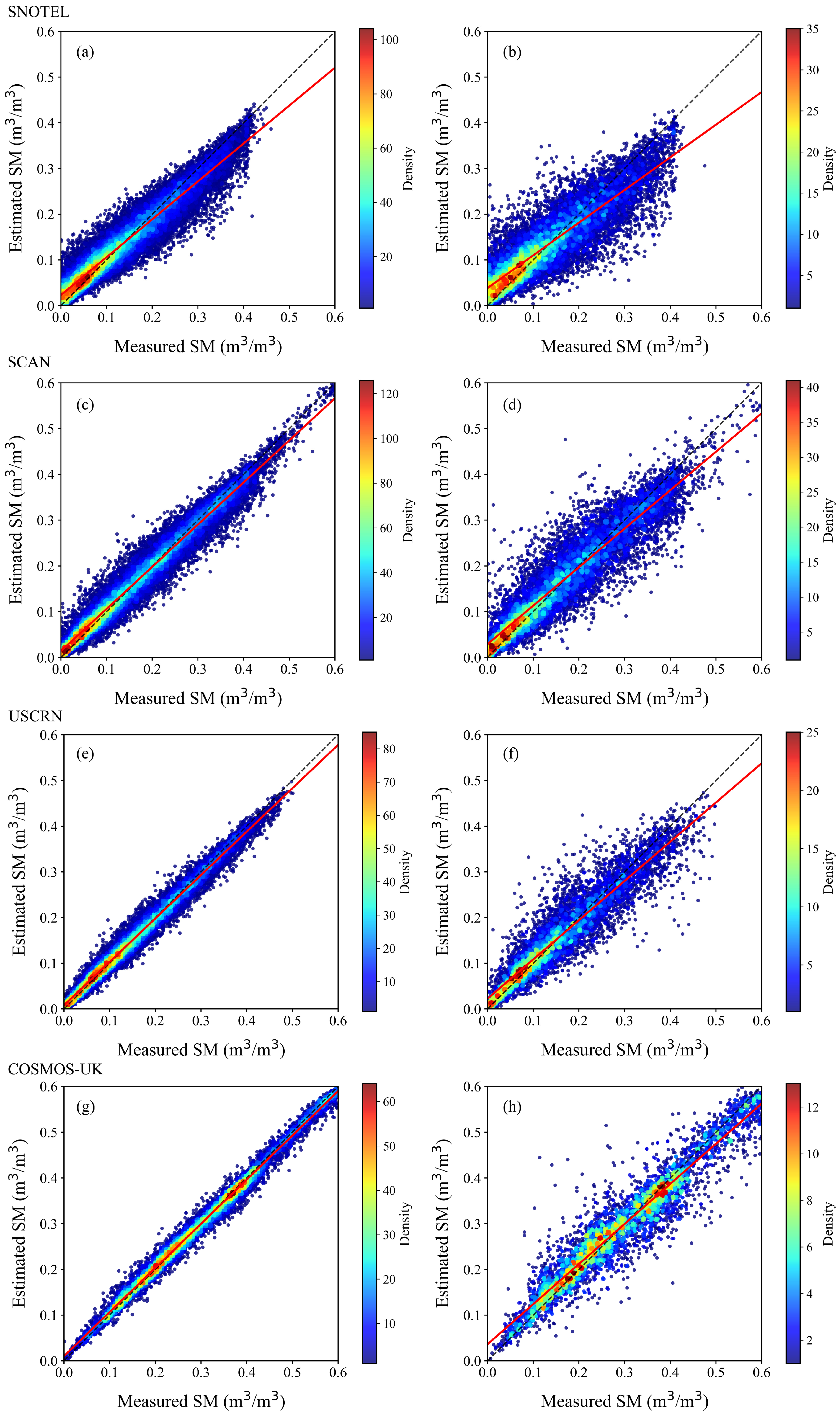
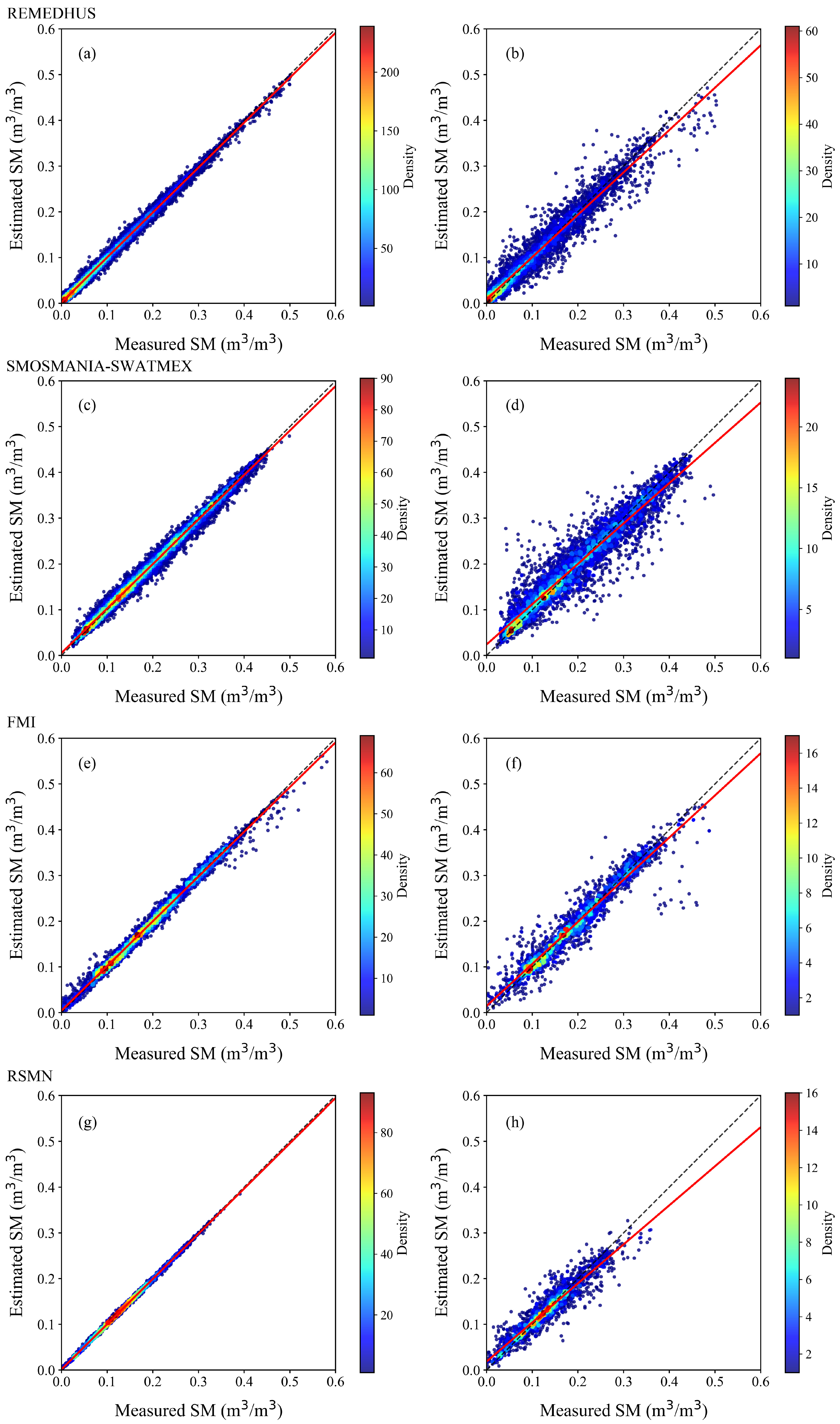
Figure 3), respectively. In all subplots, the black dashed line denotes the 1:1 reference, while the red lines represent the linear regression fit between estimated and measured SM. Color intensity represents the local density of data points, with red indicating high-density clusters and blue denoting low-density areas.
Figure 2a presents the training datasets of the global merged ISMN networks, and
Figure 2b corresponds to the validation datasets. For the training datasets, nearly all data points tightly cluster along the 1:1 reference line, and the regression line closely overlaps the 1:1 line. This visual alignment is consistent with the extremely low training bias and high R
2 reported for ISMN SM in
Table 3. The dense and narrow distribution of points confirms that the XGBoost model effectively captures the overall SM variation across the full combined dataset during training. The validation dataset exhibits linear trends similar to the training results, which verifies that the model retains an acceptable generalization capacity for the global merged dataset with negligible systematic over- or underestimation.
Figure 3 displays the training (left column: a, c, e, g) and validation (right column: b, d, f, h) density scatter plots for the first four regional monitoring networks, which contain a sufficiently large number of samples. The results for the remaining four networks are displayed in
Figure A1 of
Appendix A. For the SNOTEL network, the training scatter (
Figure 3a) shows concentrated points along the 1:1 line, but the validation subset (
Figure 3b) features pronounced point dispersion across the full SM range, with the red regression line clearly deviating from the 1:1 line at high SM values. This visual divergence matches the poorest generalization performance shown in
Table 3. For the remaining three networks, the training datasets form extremely compact and narrow bands aligned with the 1:1 line, supporting their high training accuracy. The validation scatter plots widen moderately, but maintain tighter clustering than SNOTEL’s validation results. The regression lines remain well-matched to the 1:1 reference, demonstrating mild generalization degradation without severe prediction bias.
Across both the global merged ISMN dataset and all individual local networks, the training datasets consistently form tighter clusters along the 1:1 line, whereas the validation data display broader scattering. This phenomenon reflects a well-recognized pattern in machine learning, where the model’s performance on the validation datasets is inherently lower than on the training datasets. The local networks present drastically different degrees of validation scatter dispersion. Networks with high validation R2 (e.g., COSMOS-UK) retain compact linear alignment in validation plots, while lower-performance networks (e.g., SNOTEL) show severe point divergence. Specifically, the SNOTEL network shows obvious SM underestimation within the high SM range. Its sites are mainly distributed in mountainous cold regions, where complex terrain, snow cover and snow melt processes lead to the model’s tendency to underestimate high SM values. This visual inter-network disparity corroborates the statistical conclusion that spatial domain and site-specific environmental heterogeneity fundamentally modulate the XGBoost model’s SM retrieval capacity. In the following section, the SHAP analysis will be implemented to examine how input feature importance shifts depending on the spatial domain.
4.2. Pearson Correlation Analysis of Predictor Input Features
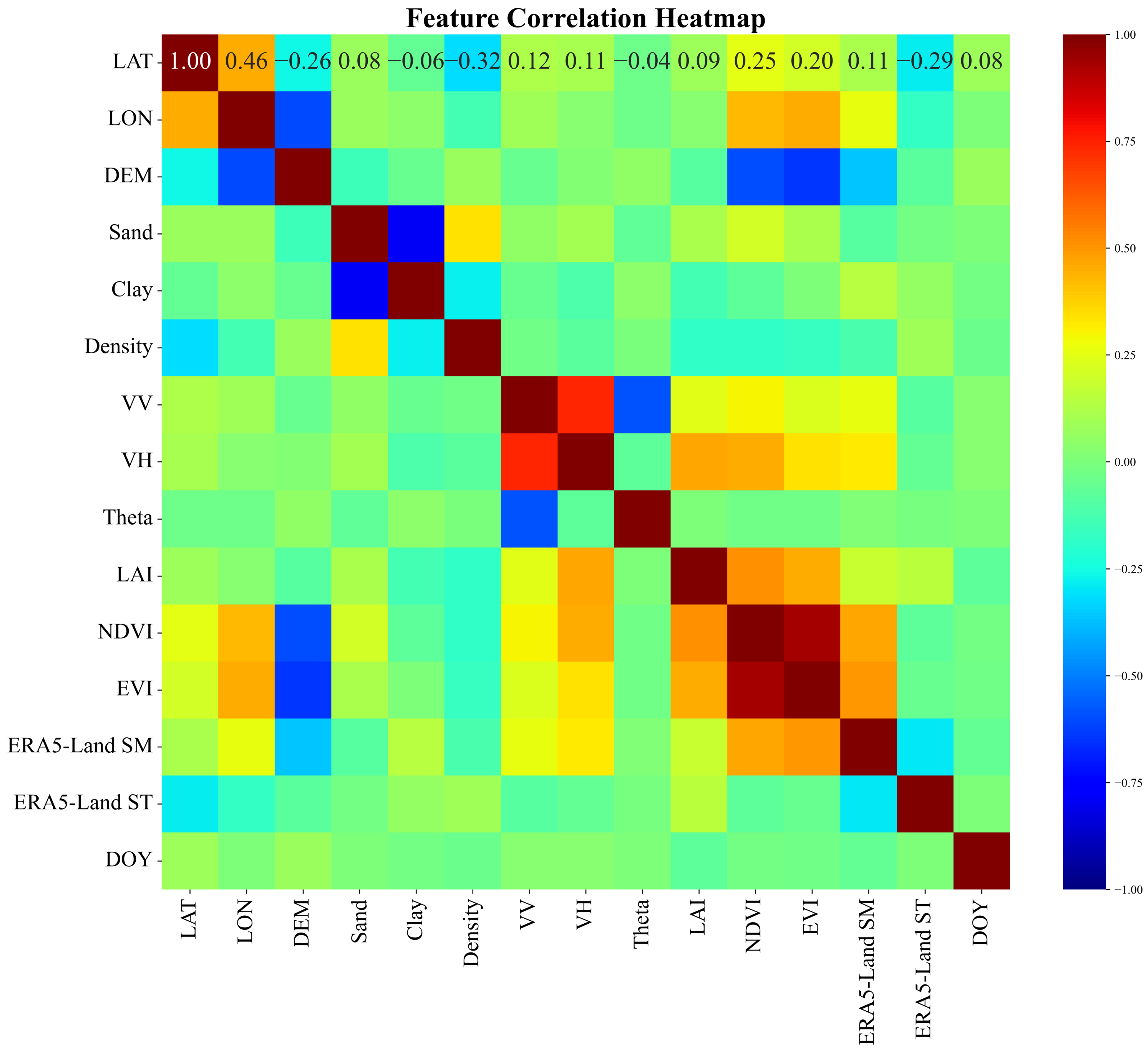
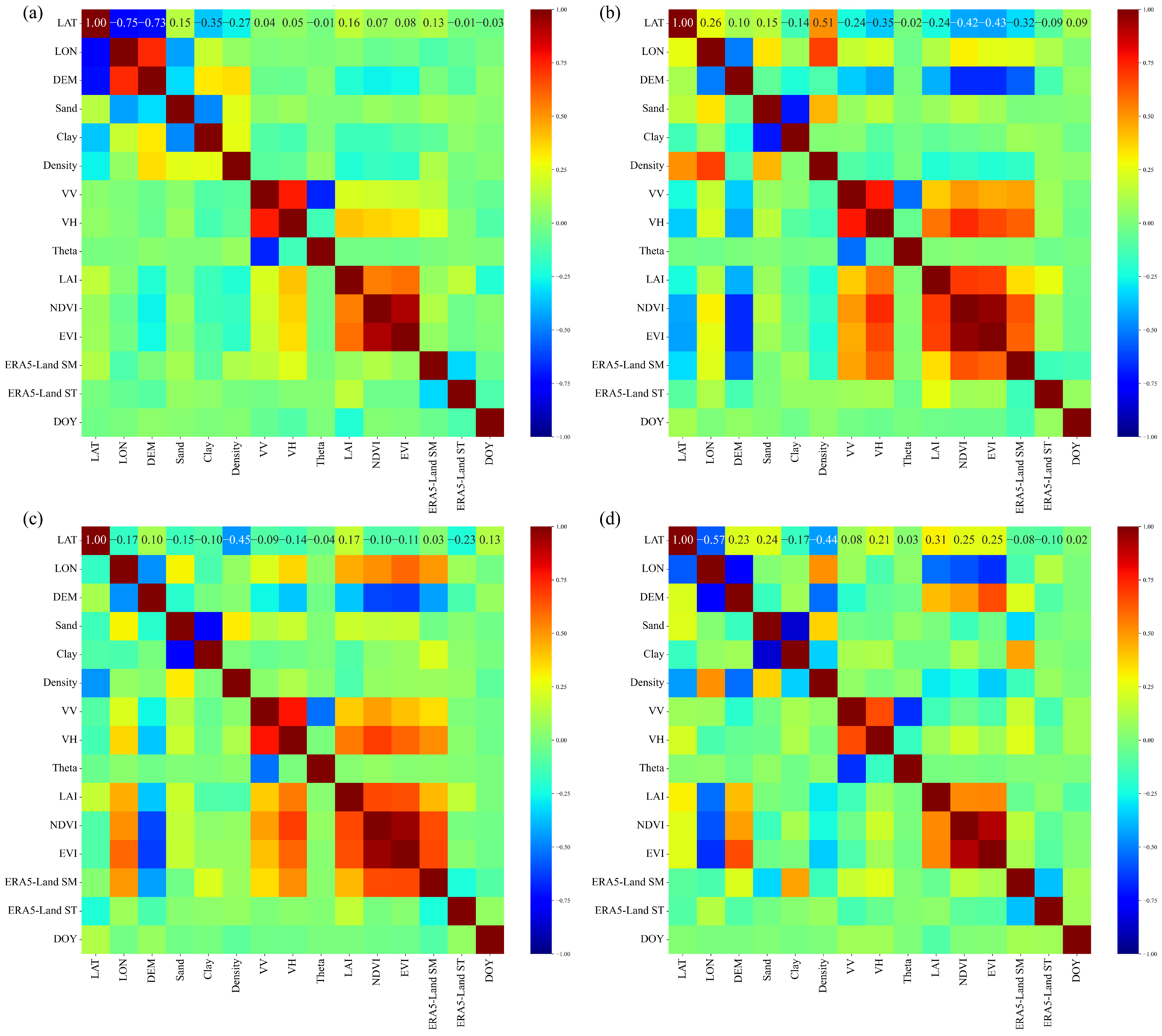
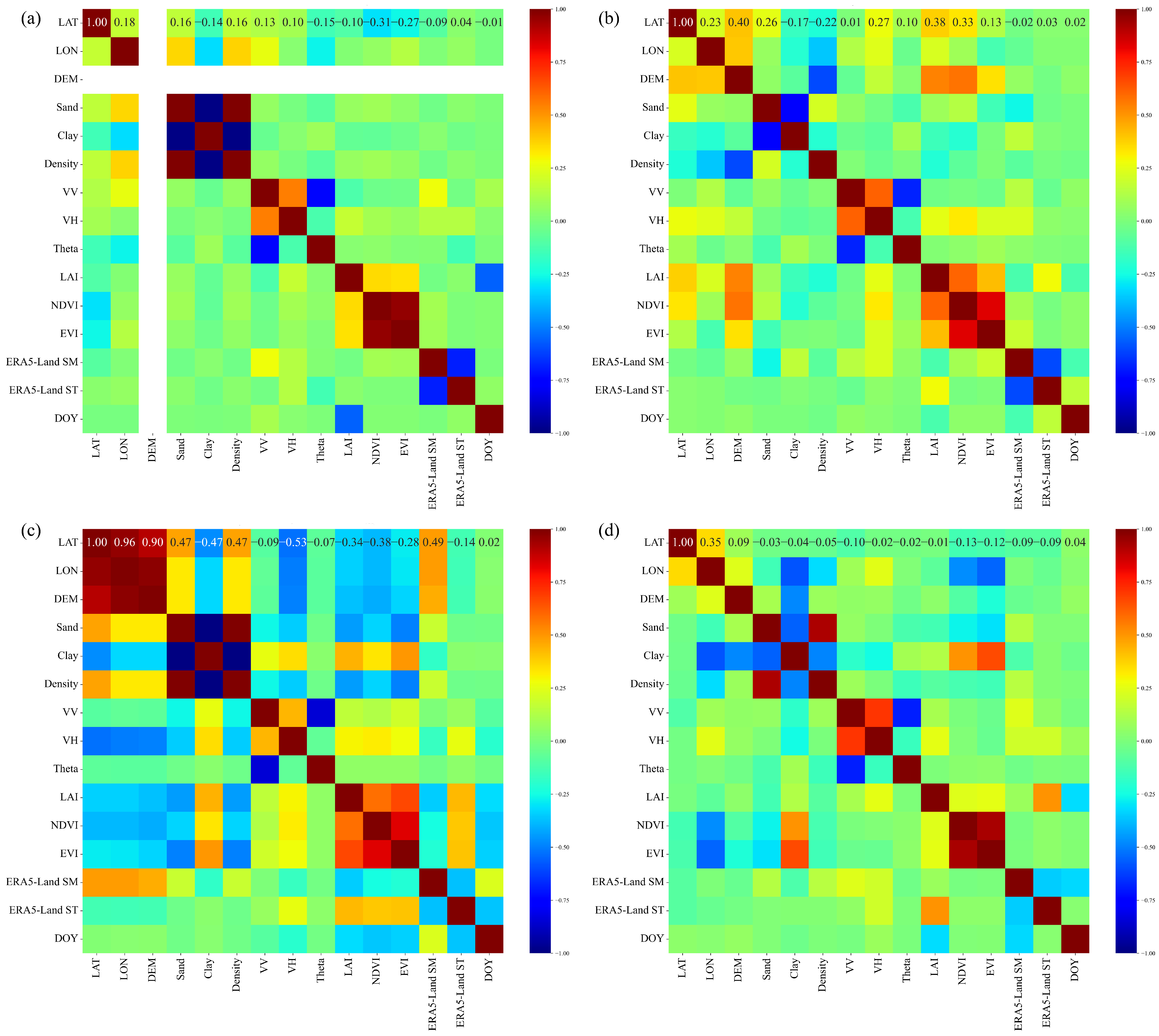
Prior to interpreting the spatial domain dependence of feature importance based on SHAP, we quantified pairwise linear correlations among all input predictors using Pearson correlation heatmaps (
Figure 4 for the merged global ISMN networks,
Figure 5 for the first four individual local networks, and
Figure A2 for the remaining four local networks). The color gradient ranges from dark blue (R = −1, strong negative correlation) to dark red (R = 1, perfect positive correlation), with yellow–green intermediate tones representing near-zero linear dependence. These results help reveal spatial domain-driven differences in covariation patterns among environmental, satellite, vegetation, and meteorological predictors across global and local regions.
Figure 4 shows a strong positive linear correlation between VV co-polarized and VH cross-polarized backscattering coefficients (R = 0.739). This inherent physical covariation arises from the consistent microwave scattering responses of surface vegetation and soil roughness across both polarizations. In addition, LAI, NDVI and EVI form a tightly correlated cluster. Notably, NDVI and EVI show a near perfect positive correlation (R = 0.932), as vegetation proxy indicators capture overlapping canopy greenness and biomass signals. Furthermore, VV and VH show highly positive correlations with vegetation proxy indicators and ERA5-Land SM, underscoring the capacity of SAR observations to be used in monitoring vegetation and soil. For the remaining predictors, nearly all pairwise correlation coefficients fall within the range of −0.30~0.30, indicating weak linear covariation. It should be noted that the strong multicollinearity among these specific feature groups will influence the SHAP attribution outputs in subsequent sections.
The four local monitoring networks demonstrate dramatically different pairwise feature correlation magnitudes and spatial covariation patterns, providing direct evidence that spatial domains reshape linear dependencies between predictive variables. The SNOTEL network presents the strongest topographic correlation signal among all subplots where LAT and DEM show an intense negative correlation. While the VV and VH radar correlation remains strongly positive (consistent with the global dataset), the covariation among vegetation indices (LAI, NDVI, EVI) weakens visibly relative to
Figure 4. In addition, VV and VH show a weak positive correlation with vegetation indicators compared to the global results in
Figure 4. Conversely, the SCAN and USCRN networks feature the most pronounced vegetation index correlation cluster, with NDVI and EVI reaching a near-perfect positive correlation. VV and VH correlation remains stable, but they have a higher positive correlation with vegetation indices and ERA5-Land SM compared to the global dataset. This suggests that vegetation and SM dominate local surface processes in this regional network. For the COSMOS-UK network, a strong VV/VH correlation and moderate vegetation index covariation are retained. However, the correlation between VV/VH, vegetation indices, and ERA5-Land SM decreases markedly compared with those from both the global dataset and other monitoring networks. This region experiences a temperate maritime climate characterized by frequent precipitation, persistent moderate SM and continuous vegetation coverage. Consequently, Sentinel-1 C-band backscatter is largely modulated by local vegetation canopy and surface roughness variations, and no longer tightly covaries with large domain reanalysis and vegetation index products.
Overall, within physically linked feature families (VV/VH, LAI/NDVI/EVI), strong positive linear correlations persist universally across both the global merged dataset and all local networks. These inherent physical covariations are invariant across spatial domains. In contrast, the cross-category correlations are highly sensitive to the spatial domain and local environmental background. This domain-driven divergence in predictor covariation provides a critical mechanistic foundation for the upcoming SHAP-based analysis of feature importance. As spatial extents shift from small local networks to a global merged dataset, changes in inter-feature linear dependencies inherently alter the relative marginal contribution of each predictor to XGBoost SM predictions, forming the core spatial domain-dependent feature importance signal explored in the following section.
4.3. SHAP Based Feature Importance
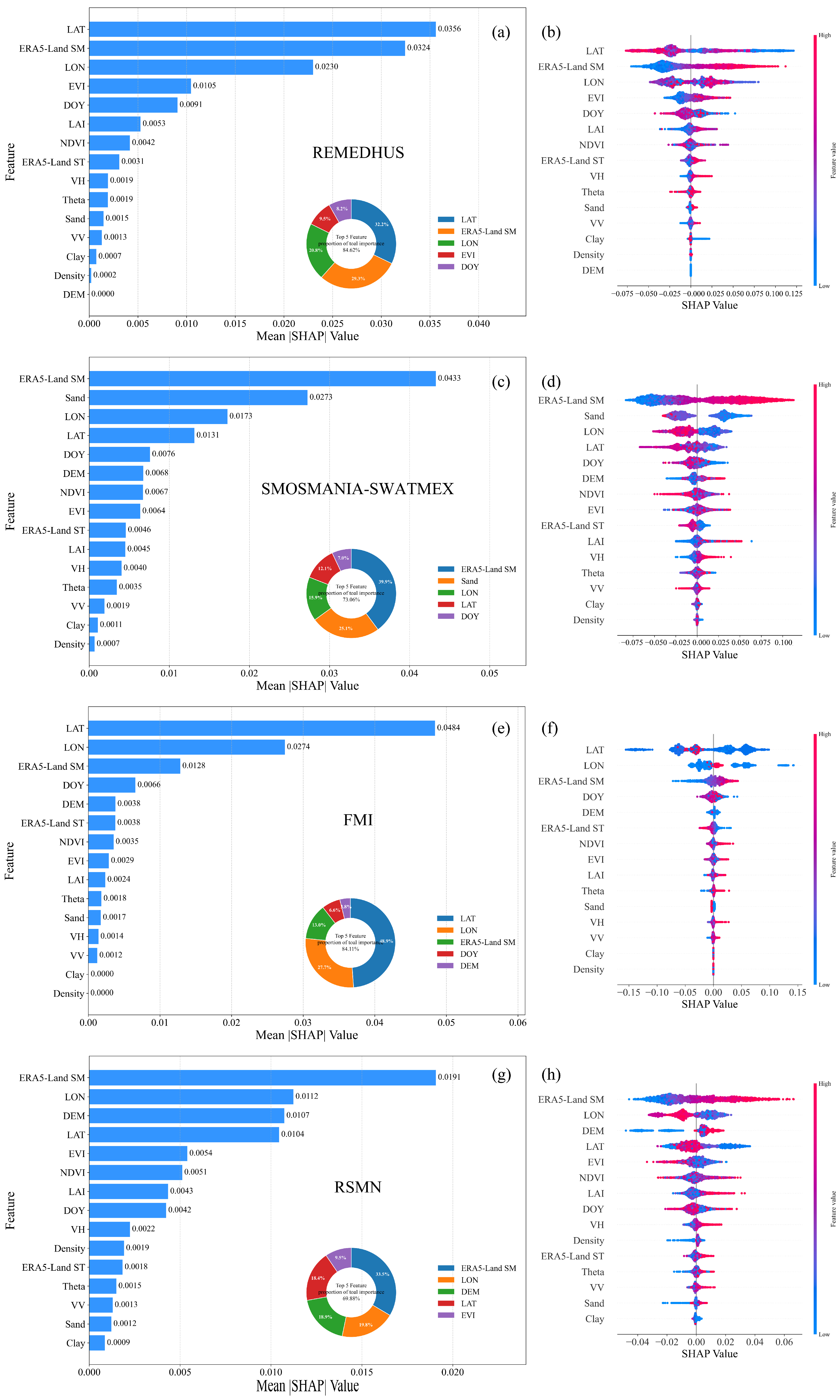
In this section, we further employ SHAP interpretability to quantify the absolute contribution (mean |SHAP|) and marginal response direction of each predictor to SM retrieval.
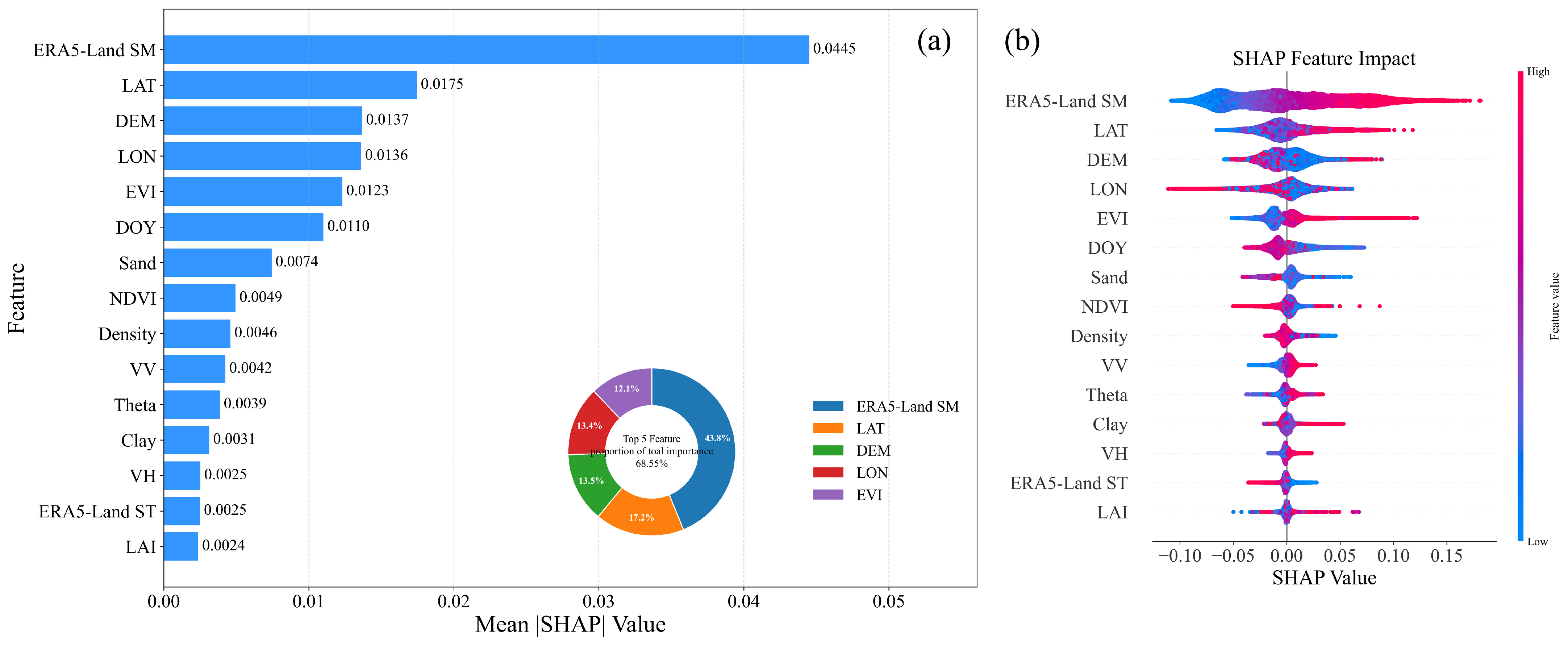
Figure 6 presents SHAP outputs for the merged global ISMN dataset.
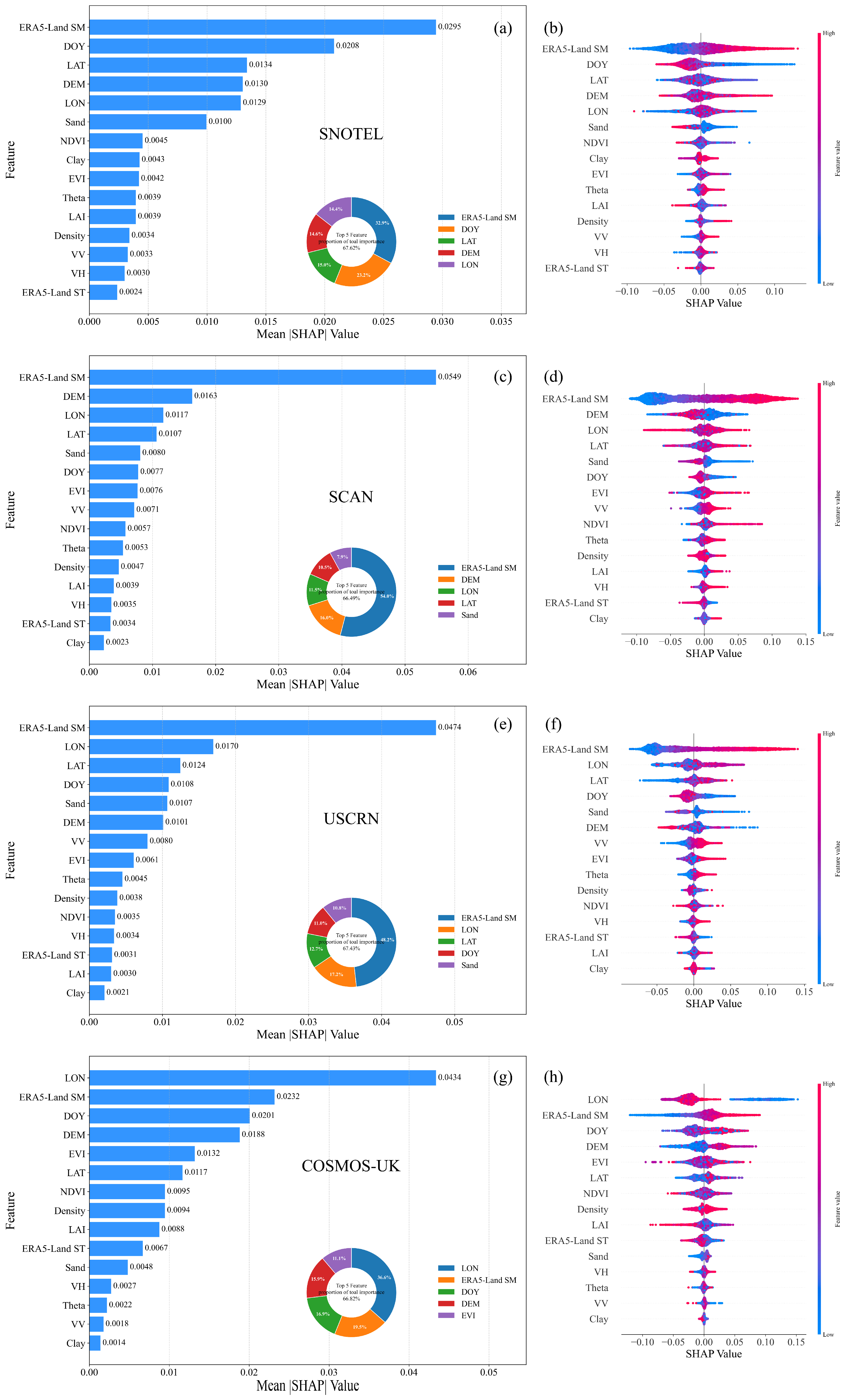
Figure 7 illustrates feature importance and SHAP dependence distributions for the first four individual networks (SNOTEL, SCAN, USCRN, and COSMOS-UK), while results for the remaining four networks are displayed in
Figure A3. The horizontal bar charts (
Figure 6a,
Figure 7a,c,e,g and
Figure A3a,c,e,g) rank predictors by their mean |SHAP| values, which quantify the overall predictive weight of each variable, and the embedded donut charts summarize the cumulative contribution of the top five dominant features. The corresponding SHAP summary beeswarm plots (
Figure 6b,
Figure 7b,d,f,h and
Figure A3b,d,f,h) visualize how varying feature values shift the predicted SM. In these plots, the horizontal axis represents the SHAP values (positive = increases predicted SM, negative = reduces predicted SM) and color gradients denote raw feature magnitude (red = high feature value, blue = low feature value). It should be noted that under strong feature collinearity, the mean |SHAP| metric redistributes predictive attribution across correlated predictors. Therefore, observed shifts in individual feature importance rankings may reflect changes in inter-feature correlation structure, not solely differences in the underlying physical SM driving mechanisms. Accordingly, we avoid overly strong causal interpretations for single-feature SHAP rankings in this study.
As shown in the horizontal bar chart (
Figure 6a), ERA5-Land SM acts as the overwhelmingly dominant predictor based on the raw mean |SHAP| values. The embedded donut subplot further presents normalized percentage contributions for visual reference. This result aligns with physical expectations, as ERA5-Land SM provides a reliable baseline estimate of SM across a wide range of global land surface conditions. The second to fifth most influential variables are LAT, DEM, LON, and EVI. Collectively, these top five predictors account for 68.55% of the total predictive power, confirming that large domain spatial patterns of SM are primarily governed by background meteorological moisture states and broad latitudinal and elevation climate gradients. By contrast, vegetation indices (LAI and NDVI), Sentinel-1A observations (VV, VH and incidence angle), soil texture properties (Sand, Clay and Density), ERA5-Land ST, and DOY exhibit far lower mean |SHAP| values. The limited contribution of these variables at the global domain level can be explained by the fact that their local effects tend to be smoothed or averaged out when datasets from widely different climate and terrain zones are combined.
The beeswarm plot (
Figure 6b) further clarifies marginal driving effects. Elevated ERA5-Land SM values produce strongly positive SHAP outputs, representing a consistent positive linear driving relationship. LAT and DEM exhibit mixed positive and negative SHAP responses, which can be largely attributed to latitudinal gradients in temperature. Furthermore, the results show that EVI, Sentinel-1A and soil parameters exert weak impacts on the global merged dataset. It should be noted that considerable sample size imbalance exists across the individual monitoring networks. For instance, SNOTEL contributes 56,366 samples, while RSMN provides only 7977 samples. The global merged dataset directly combines all available records without down sampling or equal weight stratification across networks. Therefore, the global domain model and its SHAP-derived feature importance ranking are inherently weighted toward signals from large-sample northern mid-latitude networks, rather than representing an equal contribution from each network. For future work, stratified resampling or equal weight network ensemble strategies could mitigate this imbalance, but such balancing experiments are beyond the scope of this study.
Figure 7 shows that each network demonstrates a different ranking of controlling predictors, providing definitive evidence that feature importance is highly spatially domain-dependent and modulated by site-specific environmental conditions. For the SNOTEL network, ERA5-Land SM remains the primary predictor, yet its relative dominance is drastically weakened compared to the global dataset. DOY is identified as the second most dominant predictor, with LAT, DEM, and LON ranking subsequently. The remaining features occupy the lowest importance tiers. The beeswarm plot reveals that DOY exerts a clear directional control on SM predictions locally, even though it falls to a much lower range in the global merged model. SNOTEL stations are concentrated across high-latitude and high-elevation regions of North America, where SM variability is heavily controlled by snow accumulation and melt processes, as well as intra-annual phenology. DOY effectively represents these strong local seasonal cycles, thereby gaining high local domain importance. In contrast, the global merged dataset combines observations from both hemispheres and multiple climate zones. Consequently, seasonal signals encoded by DOY become spatially incoherent: phenological and hydrological cycles are out of phase across hemispheres, and tropical sites show weak seasonal variation. These conflicting seasonal patterns partially counteract each other, reducing DOY’s marginal global predictive contribution. This rank shift illustrates how the global model prioritizes variables that capture universally consistent large domain moisture and climate gradients when reconciling divergent local environmental signals from different monitoring networks.
The SCAN network exhibits the most extreme dominance of ERA5-Land SM among all local networks, far exceeding all other predictors and even surpassing its contribution in the global dataset. DEM ranks second, while soil texture (Sand fraction) enters the top five most influential features. This pattern reflects that the background meteorological moisture is the primary control factor, while subtle topographic and soil texture differences drive local small-domain SM variability. The other features contribute minimally. For the USCRN network, ERA5-Land SM remains the dominant predictor, but LON rises to the second most influential variable. Sand fraction and DOY also rank within the top five predictors, highlighting combined controls of soil texture and seasonal climate in local SM. Vegetation and radar features remain secondary drivers. The COSMOS-UK network delivers the most dramatic domain-dependent reversal of feature importance observed in this study. Here, LON replaces ERA5-Land SM as the most important predictor, with a mean |SHAP| value of 0.0434, while ERA5-Land SM falls to second place (0.0232). DOY and DEM occupy the third and fourth positions, and EVI enters the top five key features. The beeswarm plot confirms that LON produces a wide range of positive and negative SHAP values, representing its dominant modulating effect on SM retrieval. This is driven by systematic east-west gradients of precipitation, soil and vegetation across UK. For the SMOSMANIA-SWATMEX network (
Figure A3c,d), the sand fraction ranks as the second most important predictor, contributing approximately 20% of total SHAP importance. This highlights the strong local control exerted by soil texture on surface SM variability across this French observational domain. Within this regional domain, large spatial gradients in sand content modulate SM holding capacity, infiltration, and drainage behavior. Therefore, static soil texture properties become a major driver of topsoil SM spatial heterogeneity, outweighing several dynamic satellite-derived and meteorological predictors at this local domain. This observation aligns with our core conclusion that static soil texture variables gain elevated predictive importance within local domain models.
When integrating all heterogeneous monitoring networks into a unified global dataset, ERA5-Land SM becomes the undisputed primary control. Fine domain predictors (vegetation, radar backscatter, soil texture) lose predictive weight, as their site-specific signals are smoothed and averaged across divergent environmental zones. Latitude, elevation, and longitude act as secondary drivers by capturing continental domain climate gradients. However, at individual local networks, the relative importance of ERA5-Land SM declines for some networks, and predictors tied to regionally unique landscape characteristics rise to prominence. Across different domains, Sentinel-1A radar polarizations (VV, VH), ERA5-Land ST, and LAI consistently occupy the lowest tiers of feature importance. This indicates that microwave backscatter and LAI exert weak marginal effects on the XGBoost SM retrieval, regardless of spatial extent, likely due to their collinear covariation with NDVI/EVI and ERA5-Land SM, as observed in the preceding correlation heatmaps. Collectively, the SHAP results quantitatively verify that the relative contribution of input predictors to SM retrieval based on the XGBoost model is strongly spatial-domain-dependent. The observed shifts in feature importance from global to local domains arise from the changing dominant environmental processes governing surface SM variability at different spatial extents. This provides critical guidance for optimizing predictor selection in multi-scale machine learning-based SM retrieval frameworks.
5. Discussion
5.1. Role of ERA5-SM Revealed by Ablation Experiments
In our global domain analysis and certain other local domain analyses, ERA5-Land SM exhibits the greatest SHAP-derived importance among all input predictors. However, this study should not be regarded as a conventional ERA5-Land SM downscaling exercise. The ablation experiments summarized in
Table 4 provide supportive quantitative evidence for this viewpoint. When only ERA5-Land SM is used as the predictor, the model achieves a validation R
2 of only 0.337. By contrast, the model excluding ERA5-Land SM still achieves considerable predictive accuracy, with validation R
2 reaching 0.782, using Sentinel-1 SAR, vegetation indices, static geospatial covariates (latitude, longitude, DEM), and other terrain and soil auxiliary variables. This demonstrates that satellite-derived and surface covariates carry independent predictive capacity for surface SM retrieval. When ERA5-Land SM is incorporated into the full input model, the validation R
2 is further increased to 0.820. This indicates that ERA5-Land SM delivers moderate performance improvement by acting as a coarse regional background prior. Therefore, our framework functions as a multi-source hybrid machine learning system that learns to refine the coarse reanalysis background using high-resolution satellite and surface information, rather than simply downscaling ERA5-Land SM products.
5.2. Predictor Importance on SM Retrieval
Previous SHAP-based SM modeling studies have mostly reported feature importance patterns for either a single global model or one specific study area, generally confirming the relative contributions of common SM predictors. Beyond reproducing these known patterns, the novelty of this work lies in the systematic comparisons of SHAP-derived predictor importance hierarchies across a global domain and multiple independent regional domain models. Our results demonstrate that the dominant predictors governing surface SM are not invariant, but instead change across spatial domains. We further differentiate domain stable inherent physical feature correlations from spatially variable cross-category covariations, illustrating how region-specific correlation structures can reshape SHAP-based attribution outputs. This reveals the spatial domain-dependent nature of feature importance hierarchies within multi-source SM machine learning workflows.
To mitigate interpretability challenges caused by multicollinearity among physically correlated predictors, we performed grouped feature importance analysis by summing the mean |SHAP| values for predefined collinear feature groups (
Table 5). In the global domain, the geospatial covariate group (LAT+LON+DEM) and ERA5-SM are the two most influential predictors, showing comparable aggregated importance. The vegetation group (LAI+NDVI+EVI) ranks third, whereas the Sentinel-1 radar group (VV+VH) shows relatively minor importance. However, clear regional variations are observed across different datasets. The REMEDHUS, FMI, and RSMN networks show broadly consistent patterns with the global ISMN dataset. For the SCAN and USCRN networks, ERA5-Land SM supersedes the geospatial group as the most important predictor. For the COSMOS-UK network, the geospatial group (LAT+LON+DEM) dominates model predictions, followed by the vegetation indices group (LAI+NDVI+EVI). For the SMOSMANIA-SWATMEX network, the sand fraction becomes the third most influential predictor. For the SNOTEL network, the vegetation indices group occupies the third position in predictor importance. The vegetation collinear group shows high importance in COSMOS-UK and RSMN networks, but only moderate contributions in other networks. By contrast, the radar group (VV+VH) exhibits low aggregated importance across most study domains. The higher mean |SHAP| values for the geospatial covariate group among global and local domains highlights the strong control of spatial topography on SM. The moderate mean |SHAP| values for the vegetation indices group arises from multiple physical feedbacks between vegetation and SM. These findings demonstrate that the aggregated importance of collinear feature groups is strongly region dependent. The combined effect of spatially correlated predictors (LAT+LON+DEM) is amplified when strong topographic and climatic gradients exist within a study area. Ultimately, the relative priority of predictor groups shifts with local environmental conditions, suggesting that global domain feature importance cannot be directly transferred to local domain applications.
Our SHAP-based analysis reveals persistently low marginal importance for Sentinel-1 VV and VH polarizations across most spatial domains, which appears counter intuitive considering the abundance of existing literature reporting reliable SM retrieval from C-band SAR observations. This phenomenon should not be interpreted as evidence that Sentinel-1 backscatter lacks physical sensitivity to SM. Instead, it mainly stems from the multicollinearity among input features within our multi-source XGBoost model. Predictors such as NDVI, EVI and ERA5-Land SM share strong covariation with SAR backscatter signals. Under such conditions, TreeSHAP tends to redistribute predictive attribution among correlated covariates, meaning most SM-related information contained in VV/VH is captured by other co-varying predictors. Therefore, this represents weak marginal contributions only under the current feature combination. If Sentinel-1 SAR observations were used as the primary input source, their predictive power would become more prominent. In addition, site-specific surface conditions, such as vegetation canopy structure and surface roughness, can further modulate the effective contribution of SAR signals across different regional domains.
Importantly, longitude (LON) is a static geographic coordinate and not a direct physical predictor. Its elevated importance in the COSMOS-UK network does not reflect a direct physical influence of longitude itself. Instead, LON serves as a spatial proxy for the strong west-to-east environmental gradients present across the study area. Across the UK, precipitation decreases markedly from the wet western coast toward the drier eastern interior, which further drives spatial variations in SM and vegetation status. The XGBoost model captures these consistent spatial patterns and uses LON as a surrogate variable to represent these correlated physical signals. Although location memorization effects cannot be fully excluded, the dominant contribution originates from the real east–west climatic and environmental gradients. This observation highlights a key interpretive caveat, namely, that geographic coordinates may achieve high SHAP importance when they are tightly coupled to underlying physical drivers, even though they are not physically meaningful predictors themselves.
5.3. Limitations and Outlook
This study explores the shifts in predictor importance controlling surface SM across different spatial domains based on multi-site observations from the ISMN. Nevertheless, the sample size varies substantially among individual ISMN monitoring networks. Networks with larger observation volumes contribute more samples to model training and SHAP analysis, which makes our comparative results intrinsically biased toward regions with abundant in situ records. Networks with limited sample counts may not be sufficiently represented, and their feature importance patterns could be under-captured in our outputs. Although we select eight representative networks with adequate data volumes for regional domain analysis, the uneven spatial distribution of available ground observations remains an inherent constraint of this work. Future investigations could adopt stratified sampling strategies to balance sample contributions across networks, thereby achieving more equitable comparisons of driving factor patterns among diverse regions.
Given the above-mentioned limitations, several promising directions remain for future improvement. First, further work could explore objective spatial domain thresholds to quantitatively separate global domain and regional domain modeling regimes, which would help clarify at which spatial level the dominant controlling factors of SM begin to shift. Second, the reliability of SHAP attribution should be validated under more diverse scenarios, including varying seasonal and temporal contexts. Additionally, it is necessary to evaluate how different machine learning algorithms may alter SHAP-derived feature importance outputs. Third, regarding validation strategies, future studies should adopt more robust evaluation schemes such as leave-year-out, leave-station-out and spatially blocked cross-validation to mitigate spatiotemporal leakage. Grouped feature block importance analysis can also be implemented to reduce the attribution bias caused by multicollinearity. Finally, more complete observation datasets are required, and hydrometeorological time-lag effects should be incorporated into the modeling workflow. Consistent with our earlier discussion, stratified sampling strategies should also be considered to balance sample contributions across networks and achieve fairer inter-regional comparisons of SM driving patterns.
6. Conclusions
This study develops an interpretable XGBoost and SHAP framework to quantitatively describe the spatial domain dependence evolution of predictor importance for machine learning-based SM retrieval, using global multiple networks’ in situ SM observations from the ISMN covering 2017–2024. The model performance comparison between the unified global model and the independent regional monitoring networks model has verified that the globally trained model exhibits a reduced risk of over-fitting and better cross-domain stability across diverse land surface conditions. Conversely, while many regional domain models achieve higher absolute retrieval accuracy within their specific locals, their overall performance remains constrained by local surface environmental heterogeneity.
Pearson correlation analysis demonstrated that physically linked feature groups (e.g., Sentinel-1A VV/VH polarizations, and LAI/NDVI/EVI vegetation indices) maintain stable high collinearity across different domains. However, cross-category correlations among radar, vegetation and meteorological predictors are highly sensitive to study extent and regional background conditions. SHAP-based feature importance quantification further confirmed evident domain-dependent differentiations among dominant controlling factors. At the global domain level, ERA5-Land SM acts as the dominant predictor, contributing nearly 44% of total predictive power, with geospatial gradients (latitude, longitude, elevation) serving as secondary regulators. Localized covariates including radar signals, vegetation indices and soil texture may exhibit reduced marginal predictive weight. This reduction partly originates from the spatial averaging of heterogeneous surface signals and inter-feature covariation across predictors.
At regional domains, the feature importance of ERA5-Land SM exhibits a heterogeneous behavior relative to the global pooled model. It remains the dominant predictive feature for the SNOTEL, SCAN, USCRN SMOSMANIA-SWATMEN and RSMN networks, achieving even higher importance for the SCAN network than in the global model. Nevertheless, for the COSMOS-UK network, longitude (LON) overtakes ERA5-Land SM to become the leading predictor, while latitude (LAT) replaces it as the top feature for the REMEDHUS and FMI networks. Group feature importance analysis highlights that the relative contributions of predictor groups shift substantially between global and regional domains. Within our multi-source modeling framework, Sentinel-1A radar backscatter, surface soil temperature and LAI exhibit relatively low marginal independent contributions across most spatial domains, largely due to collinearity with other vegetation and SM-related covariates. However, this does not imply that these radar observations contain no SM-relevant physical signals.
These findings provide clear spatial domains and adaptive guidance for predictor selection in SM modeling. For global domain SM retrieval frameworks, ERA5-Land SM should be retained as the core input, while fine domain local predictors can be simplified to reduce computational cost. Regional downscaling models, on the other hand, require targeted feature screening that prioritizes seasonal, topographic and soil texture variables to capture local SM variability. Moreover, highly collinear vegetation and radar features can be selectively removed to streamline model training without significant accuracy loss. Ultimately, this work advances the interpretability of machine learning-based SM retrieval, and offers a scalable feature optimization strategy for generating high-resolution SM products under diverse global land surface conditions.