Figure 1.
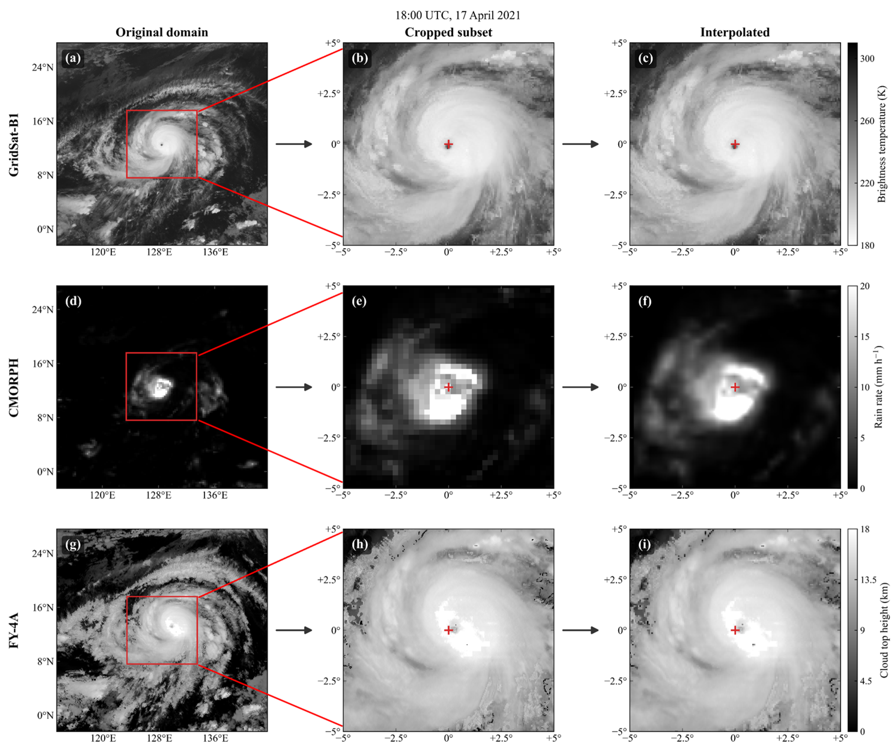
Regional extraction and spatial interpolation of three-channel satellite observation data for the TC case 2021102N06144 at 18:00 UTC on 17 April 2021. Panels (a–c), (d–f), and (g–i) correspond to GridSat-B1 infrared brightness temperature (K), CMORPH precipitation rate (mm h−1), and FY-4A cloud-top height (km), respectively. The left, middle, and right columns represent the original observation domain, the TC-centered cropped subset, and the interpolated model input, respectively. The red rectangle indicates the 10° × 10° TC-centered extraction region shown in the following two columns. Owing to different native resolutions, the cropped subsets contain 143 × 143, 40 × 40, and 263 × 267 grid points for GridSat-B1, CMORPH, and FY-4A CTH, respectively; all variables are finally resampled to a unified 143 × 143 grid for model input.
Figure 1.
Regional extraction and spatial interpolation of three-channel satellite observation data for the TC case 2021102N06144 at 18:00 UTC on 17 April 2021. Panels (a–c), (d–f), and (g–i) correspond to GridSat-B1 infrared brightness temperature (K), CMORPH precipitation rate (mm h−1), and FY-4A cloud-top height (km), respectively. The left, middle, and right columns represent the original observation domain, the TC-centered cropped subset, and the interpolated model input, respectively. The red rectangle indicates the 10° × 10° TC-centered extraction region shown in the following two columns. Owing to different native resolutions, the cropped subsets contain 143 × 143, 40 × 40, and 263 × 267 grid points for GridSat-B1, CMORPH, and FY-4A CTH, respectively; all variables are finally resampled to a unified 143 × 143 grid for model input.
Figure 2.
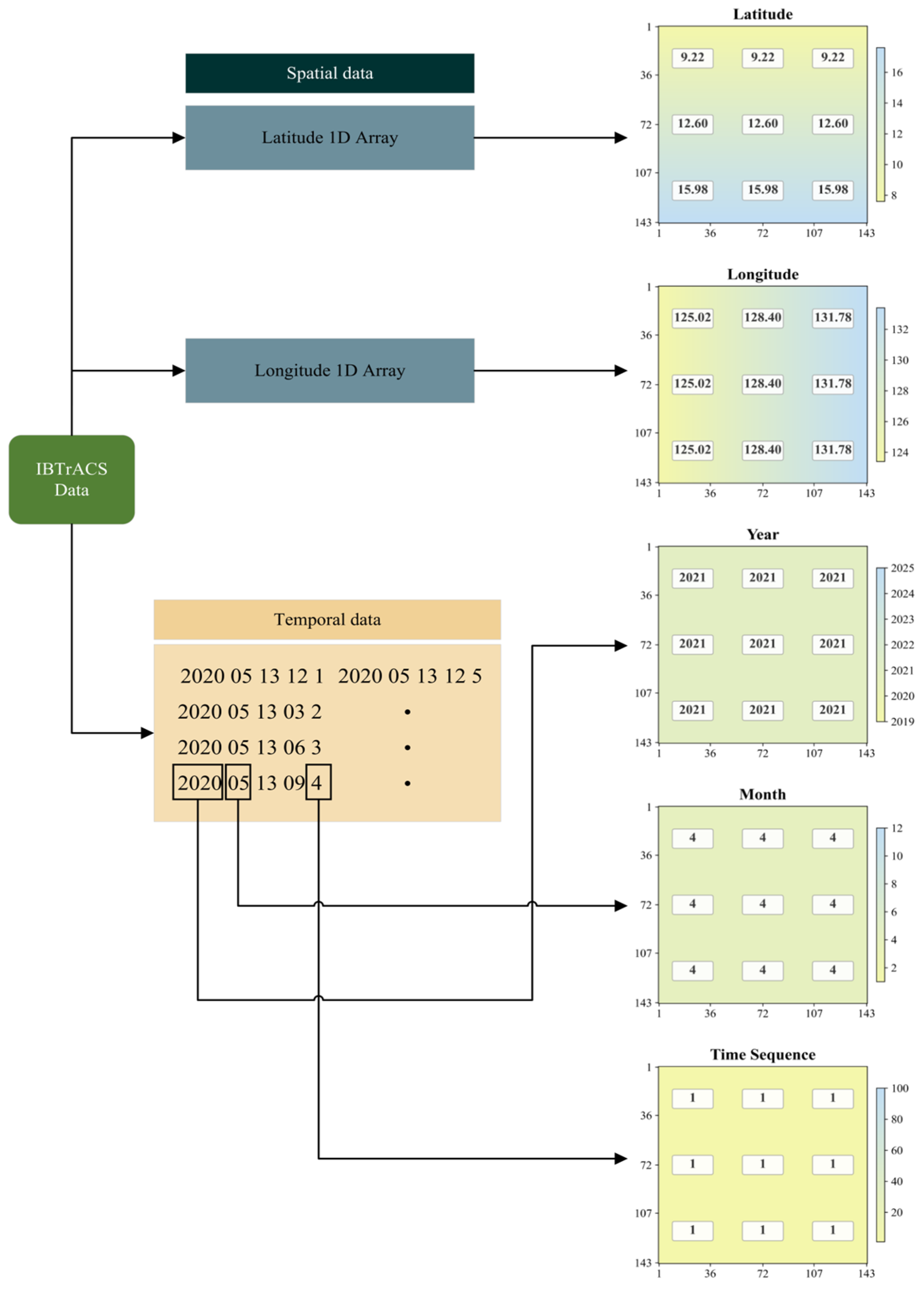
Spatiotemporal independent field variables of the five additional channels (Latitude, Longitude, Year, Month, and time sequence) generated from IBTrACS best-track data.
Figure 2.
Spatiotemporal independent field variables of the five additional channels (Latitude, Longitude, Year, Month, and time sequence) generated from IBTrACS best-track data.
Figure 3.
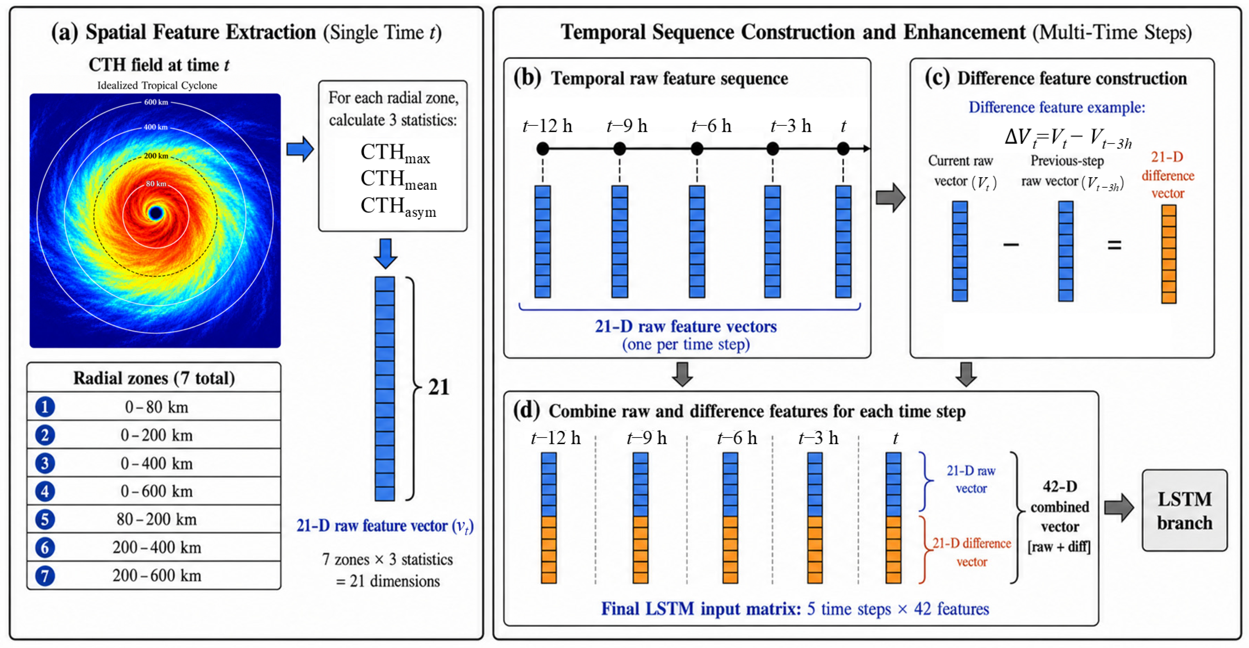
Construction of the CTH temporal feature sequence for the LSTM branch. (a) Extraction of 21-dimensional CTH statistical features from seven TC-centered radial ranges at a single time step. (b) Construction of a five-step temporal sequence over the preceding 12 h using CTH feature vectors at t − 12 h, t − 9 h, t − 6 h, t − 3 h, and t. (c) Calculation of adjacent-time-step difference features to represent the temporal evolution of CTH. (d) Concatenation of raw and difference features to generate the final 5 × 42 LSTM input matrix.
Figure 3.
Construction of the CTH temporal feature sequence for the LSTM branch. (a) Extraction of 21-dimensional CTH statistical features from seven TC-centered radial ranges at a single time step. (b) Construction of a five-step temporal sequence over the preceding 12 h using CTH feature vectors at t − 12 h, t − 9 h, t − 6 h, t − 3 h, and t. (c) Calculation of adjacent-time-step difference features to represent the temporal evolution of CTH. (d) Concatenation of raw and difference features to generate the final 5 × 42 LSTM input matrix.
Figure 4.
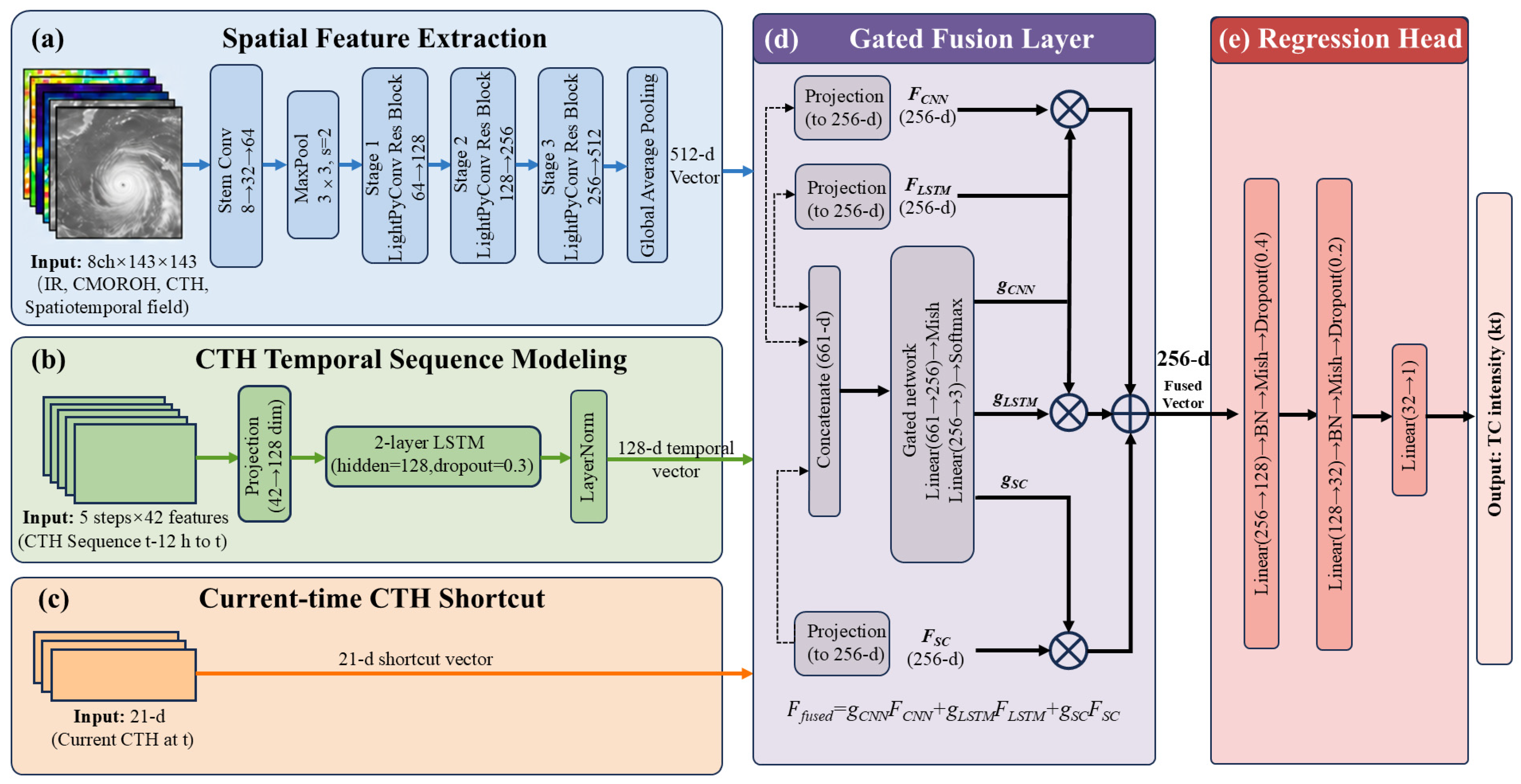
Overall architecture of the proposed CTH-TCNet for tropical cyclone intensity estimation. (a) Spatial feature extraction branch, where eight-channel 143 × 143 input fields, including infrared brightness temperature, CMORPH precipitation, CTH, and auxiliary spatiotemporal fields, are encoded by a lightweight pyramidal convolutional residual network to obtain a 512-dimensional spatial feature vector. (b) CTH temporal sequence modeling branch, where the five-time-step CTH radial statistical feature sequence from t − 12 h to t is projected and fed into a two-layer LSTM to capture the historical evolution of the upper-level cloud structure. (c) Current-time CTH shortcut branch, which directly preserves the 21-dimensional CTH radial statistics at the target time step. (d) Gated fusion layer, where the three branch features are projected into a unified feature space and adaptively weighted by learned gating coefficients. (e) Regression head, which maps the fused feature vector to the estimated TC intensity in kt. Here, , , and denote the projected feature representations of the spatial, temporal, and shortcut branches, respectively; , , and denote their corresponding gating coefficients; and denotes the final fused feature representation. The multiplication and addition symbols indicate branch-wise weighting and weighted summation, respectively.
Figure 4.
Overall architecture of the proposed CTH-TCNet for tropical cyclone intensity estimation. (a) Spatial feature extraction branch, where eight-channel 143 × 143 input fields, including infrared brightness temperature, CMORPH precipitation, CTH, and auxiliary spatiotemporal fields, are encoded by a lightweight pyramidal convolutional residual network to obtain a 512-dimensional spatial feature vector. (b) CTH temporal sequence modeling branch, where the five-time-step CTH radial statistical feature sequence from t − 12 h to t is projected and fed into a two-layer LSTM to capture the historical evolution of the upper-level cloud structure. (c) Current-time CTH shortcut branch, which directly preserves the 21-dimensional CTH radial statistics at the target time step. (d) Gated fusion layer, where the three branch features are projected into a unified feature space and adaptively weighted by learned gating coefficients. (e) Regression head, which maps the fused feature vector to the estimated TC intensity in kt. Here, , , and denote the projected feature representations of the spatial, temporal, and shortcut branches, respectively; , , and denote their corresponding gating coefficients; and denotes the final fused feature representation. The multiplication and addition symbols indicate branch-wise weighting and weighted summation, respectively.

Figure 5.
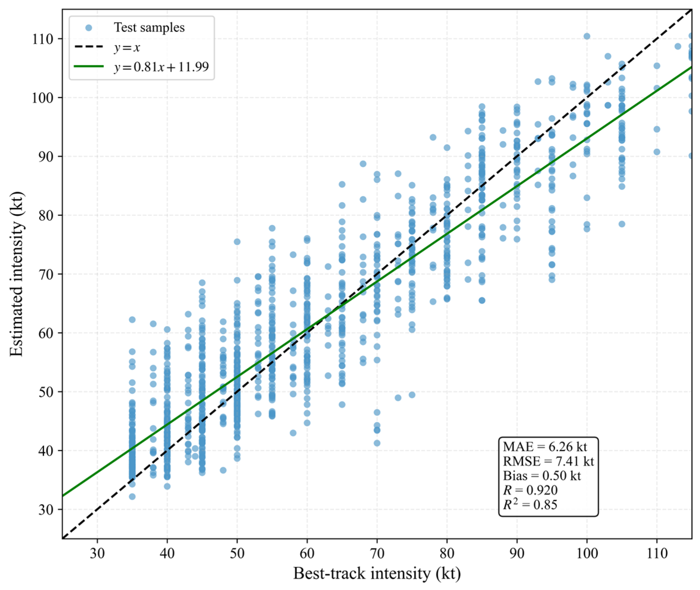
Overall intensity estimation performance of the optimal CTH-TCNet on the independent test set. Scatter points represent test samples, the black dashed line denotes the y = x reference line, and the green solid line represents the ordinary least squares linear fit between the model-estimated intensity and the IBTrACS best-track intensity.
Figure 5.
Overall intensity estimation performance of the optimal CTH-TCNet on the independent test set. Scatter points represent test samples, the black dashed line denotes the y = x reference line, and the green solid line represents the ordinary least squares linear fit between the model-estimated intensity and the IBTrACS best-track intensity.
Figure 6.
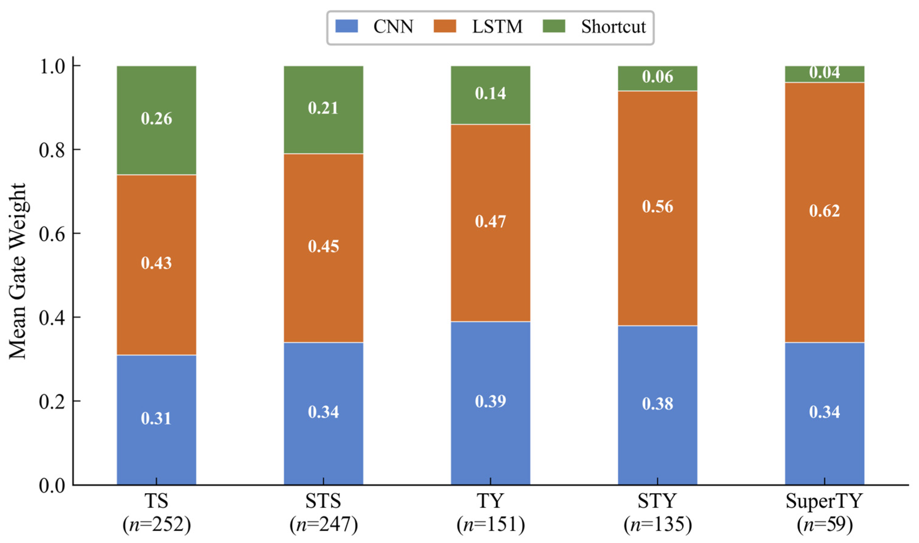
Mean gate-weight allocation among the three fusion branches of CTH-TCNet across TC intensity categories. The stacked bars represent the relative weights assigned to the CNN spatial branch, LSTM CTH temporal branch, and current-time CTH shortcut branch for each intensity category; numerical labels indicate the category-averaged gate weights, and n denotes the number of test samples included in the gating-weight analysis for each category.
Figure 6.
Mean gate-weight allocation among the three fusion branches of CTH-TCNet across TC intensity categories. The stacked bars represent the relative weights assigned to the CNN spatial branch, LSTM CTH temporal branch, and current-time CTH shortcut branch for each intensity category; numerical labels indicate the category-averaged gate weights, and n denotes the number of test samples included in the gating-weight analysis for each category.
Figure 7.
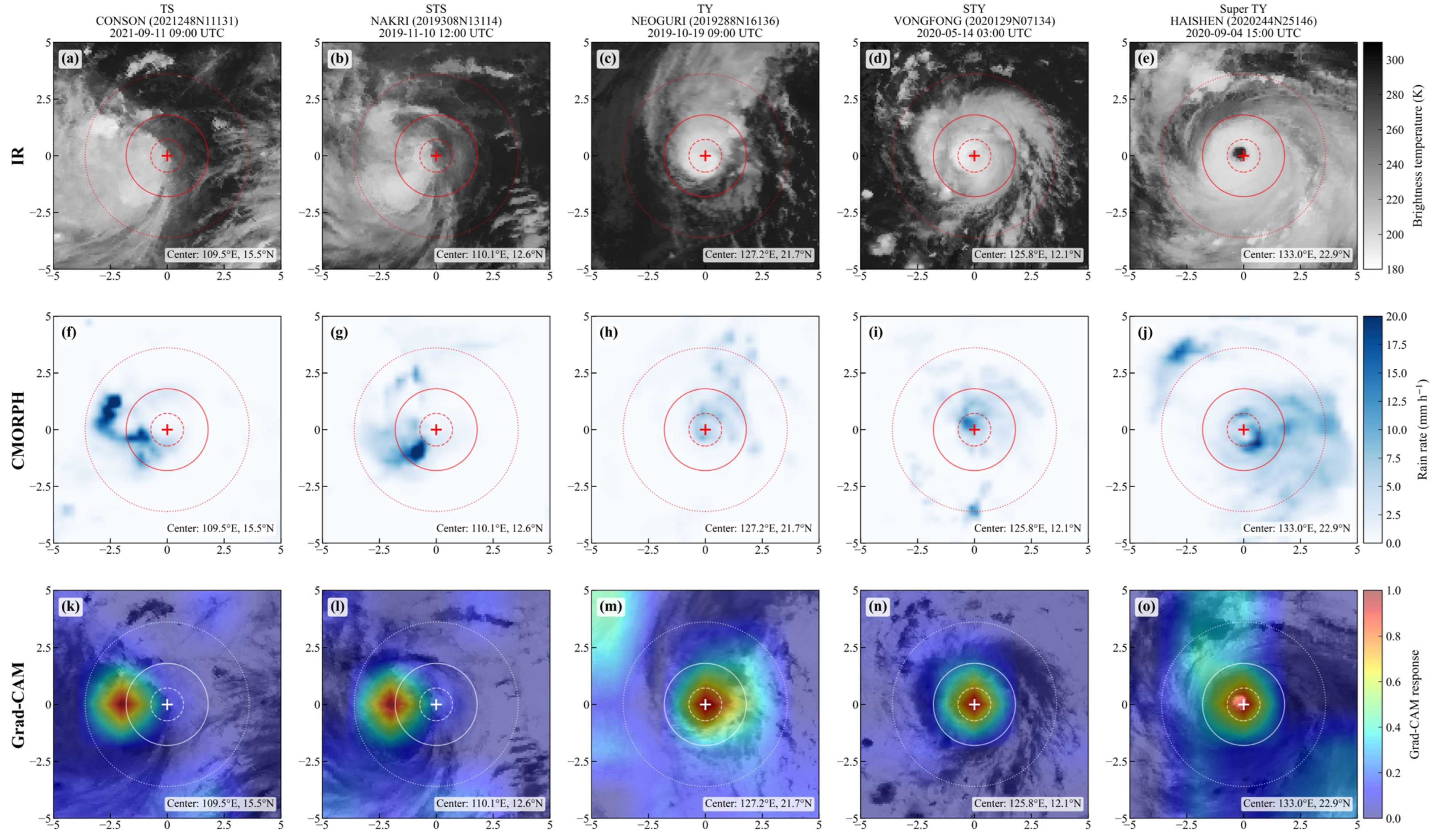
Grad-CAM visualization of CNN spatial attention for selected low-error TC samples across different intensity categories. Columns represent TS, STS, TY, STY, and Super TY samples, respectively. The first row (a–e) shows IR brightness temperature fields, the second row (f–j) shows CMORPH precipitation fields, and the third row (k–o) shows normalized Grad-CAM responses overlaid on IR imagery. The cross marks the TC center, and the concentric circles indicate radial distances of 80 km, 200 km, and 400 km from the center. Warmer colors in the Grad-CAM maps denote higher model responses, indicating the spatial regions that the CNN branch focuses on during TC intensity estimation.
Figure 7.
Grad-CAM visualization of CNN spatial attention for selected low-error TC samples across different intensity categories. Columns represent TS, STS, TY, STY, and Super TY samples, respectively. The first row (a–e) shows IR brightness temperature fields, the second row (f–j) shows CMORPH precipitation fields, and the third row (k–o) shows normalized Grad-CAM responses overlaid on IR imagery. The cross marks the TC center, and the concentric circles indicate radial distances of 80 km, 200 km, and 400 km from the center. Warmer colors in the Grad-CAM maps denote higher model responses, indicating the spatial regions that the CNN branch focuses on during TC intensity estimation.
Figure 8.
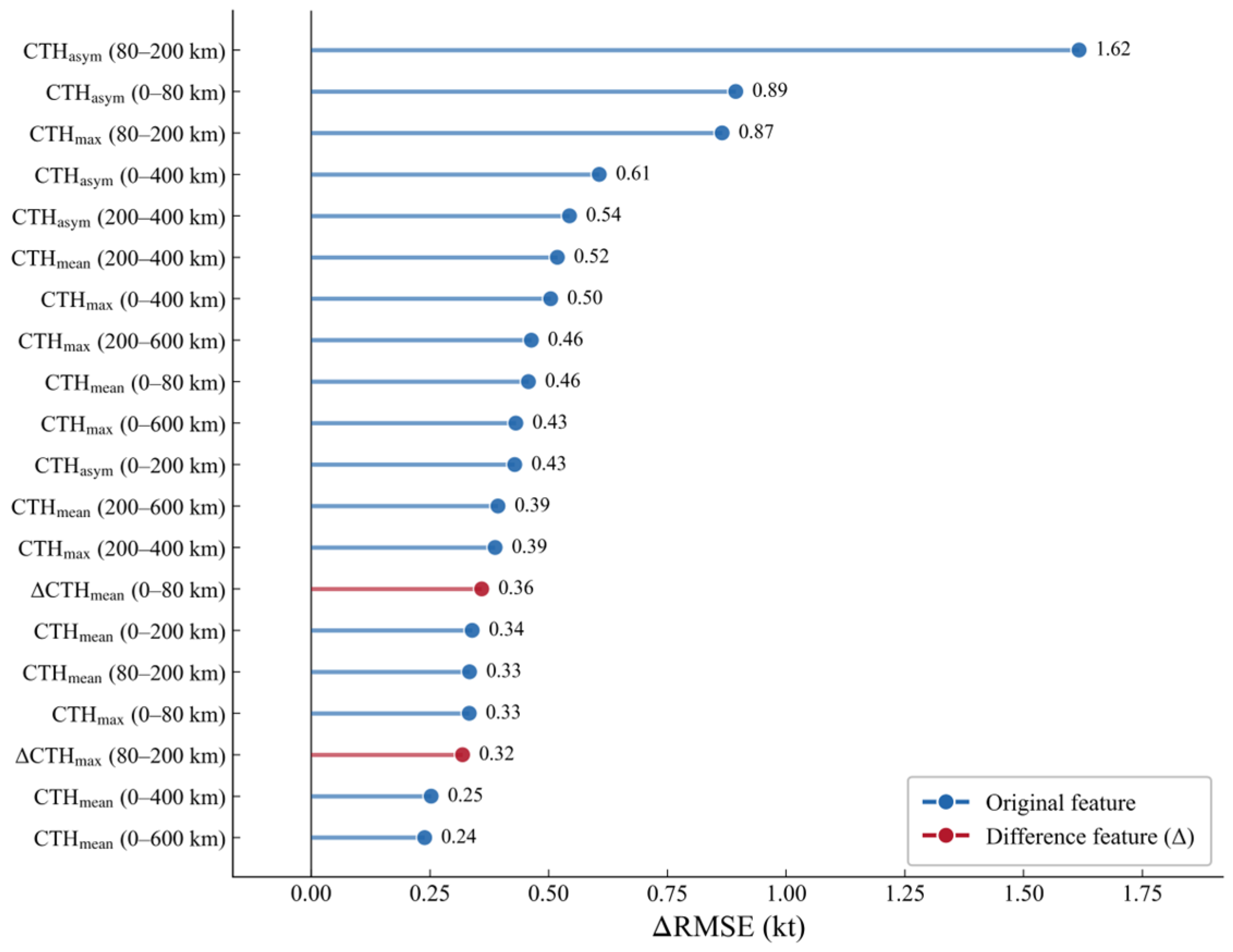
Permutation importance of the top 20 CTH input features in the LSTM temporal branch. Feature importance is measured by the increase in RMSE (ΔRMSE, kt) after randomly permuting each feature across test samples; therefore, a larger ΔRMSE indicates a stronger contribution to TC intensity estimation. Blue markers denote original CTH statistical features, and red markers denote adjacent-time-step CTH difference features. Results are averaged across three independent random seeds.
Figure 8.
Permutation importance of the top 20 CTH input features in the LSTM temporal branch. Feature importance is measured by the increase in RMSE (ΔRMSE, kt) after randomly permuting each feature across test samples; therefore, a larger ΔRMSE indicates a stronger contribution to TC intensity estimation. Blue markers denote original CTH statistical features, and red markers denote adjacent-time-step CTH difference features. Results are averaged across three independent random seeds.
Figure 9.
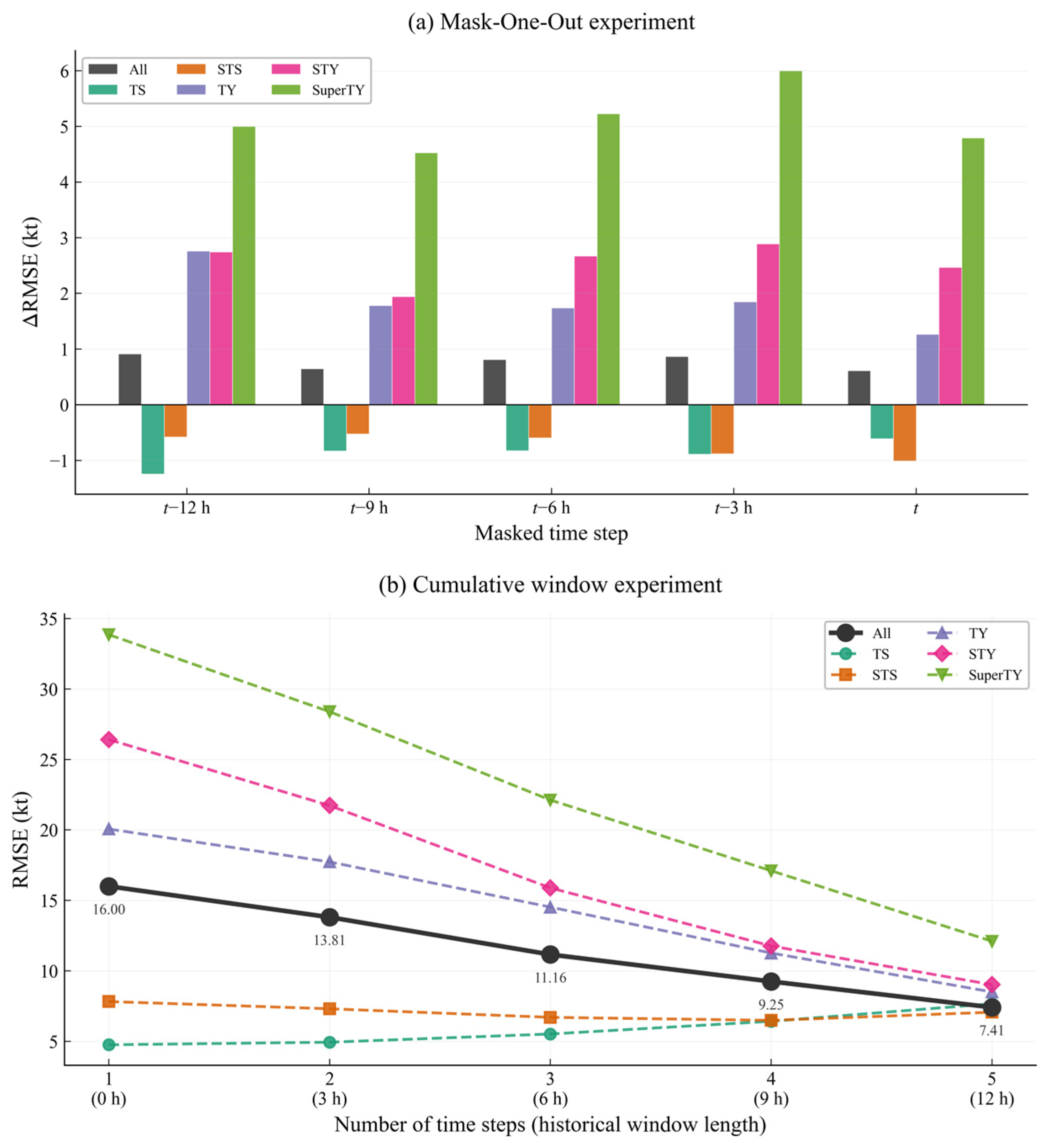
Intensity-stratified temporal ablation analysis of the CTH statistical feature sequence in the LSTM branch. The temporal input consists of five consecutive observations at 3-h intervals spanning the current time and the preceding 12 h: t − 12, t − 9, t − 6, t − 3, and t. Results are presented for all test samples and separately for the TS, STS, TY, STY, and Super TY categories. (a) Mask-One-Out experiment, in which the CTH features at one time step are set to zero while the remaining time steps are retained. The bars show the change in RMSE relative to the complete five-step input (, kt). Positive values indicate performance degradation after masking and therefore a positive contribution of the removed time step, whereas negative values indicate that masking reduces the RMSE. (b) Cumulative Window experiment, in which the input sequence begins with the current time step t, followed by the progressive addition of t − 3, t − 6, t − 9, and t − 12. The lines show the RMSE as the input sequence increases from one to five time steps, corresponding to historical window lengths of 0–12 h.
Figure 9.
Intensity-stratified temporal ablation analysis of the CTH statistical feature sequence in the LSTM branch. The temporal input consists of five consecutive observations at 3-h intervals spanning the current time and the preceding 12 h: t − 12, t − 9, t − 6, t − 3, and t. Results are presented for all test samples and separately for the TS, STS, TY, STY, and Super TY categories. (a) Mask-One-Out experiment, in which the CTH features at one time step are set to zero while the remaining time steps are retained. The bars show the change in RMSE relative to the complete five-step input (, kt). Positive values indicate performance degradation after masking and therefore a positive contribution of the removed time step, whereas negative values indicate that masking reduces the RMSE. (b) Cumulative Window experiment, in which the input sequence begins with the current time step t, followed by the progressive addition of t − 3, t − 6, t − 9, and t − 12. The lines show the RMSE as the input sequence increases from one to five time steps, corresponding to historical window lengths of 0–12 h.

Figure 10.
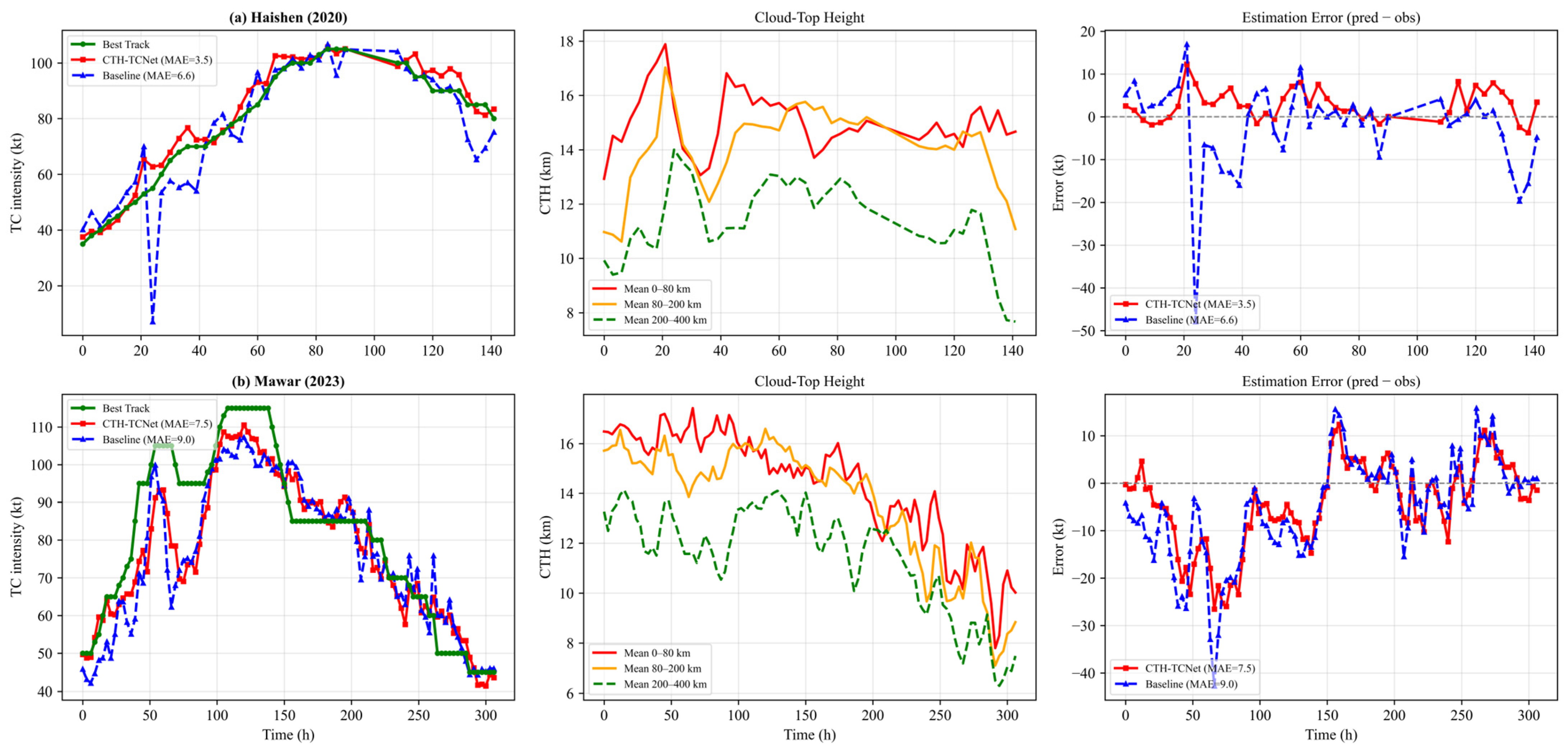
Representative case studies of TC intensity estimation and CTH evolution for (a) Haishen (2020) and (b) Mawar (2023). The left column compares the best-track intensity with estimates from CTH-TCNet (Experiment H) and the no-CTH baseline (Experiment B); the middle column shows the temporal evolution of mean CTH within 0–80, 80–200, and 200–400 km radial regions; and the right column presents the corresponding time-step estimation errors (estimated minus observed). The MAE for each model over the entire case is reported in the legends.
Figure 10.
Representative case studies of TC intensity estimation and CTH evolution for (a) Haishen (2020) and (b) Mawar (2023). The left column compares the best-track intensity with estimates from CTH-TCNet (Experiment H) and the no-CTH baseline (Experiment B); the middle column shows the temporal evolution of mean CTH within 0–80, 80–200, and 200–400 km radial regions; and the right column presents the corresponding time-step estimation errors (estimated minus observed). The MAE for each model over the entire case is reported in the legends.
Table 1.
Configuration of the eight-channel image input to the model.
Table 1.
Configuration of the eight-channel image input to the model.
| Channel | Variable | Data Source | Native Resolution | Value Range |
|---|
| 1 | Infrared brightness temperature | GridSat-B1 | 8 km/3 h | 180–310 K |
| 2 | Precipitation rate | CMORPH | 25 km/1 h | ≥0 mm/h |
| 3 | CTH | FY-4A/B | 4 km/15 min | 0–20,000 m |
| 4 | Year | Metadata encoding | — | 2019–2025 |
| 5 | Month | Metadata encoding | — | 1–12 |
| 6 | Time sequence | Metadata encoding | — | ≥1 |
| 7 | Latitude | Coordinate grid | Per pixel | 5°S–55°N |
| 8 | Longitude | Coordinate grid | Per pixel | 90°E–160°E |
Table 2.
Dataset partitioning and sample statistics under the three random seeds.
Table 2.
Dataset partitioning and sample statistics under the three random seeds.
| Random Seed | Training TCs | Training Time Steps | Validation TCs | Validation Time Steps | Test TCs | Test Time Steps |
|---|
| 214 | 124 | 3199 | 16 | 478 | 16 | 427 |
| 531 | 124 | 3355 | 16 | 342 | 16 | 407 |
| 654 | 124 | 3397 | 16 | 349 | 16 | 358 |
Table 3.
Common experimental settings and main hyperparameter settings for model training.
Table 3.
Common experimental settings and main hyperparameter settings for model training.
| Parameter | Setting |
|---|
| Optimizer | AdamW |
| Initial learning rate | 5 × 10⁻⁴ |
| Batch size | 32 |
| Early stopping patience | 35 epochs |
| Maximum epochs | 300 |
| Weight decay | 5 × 10⁻⁴ |
| Loss function | Hybrid intensity-weighted Huber–MSE loss |
| Random seeds | 214, 531, 654 |
| Number of repeated runs | 3 per configuration |
Table 4.
Configurations and test-set performance of the nine ablation experiments designed to disentangle the contributions of the two-dimensional CTH spatial field, historical CTH evolution, and current-time CTH statistics. Performance metrics are reported as mean ± standard deviation over three independent runs. The corresponding TC-level 95% bootstrap confidence intervals are provided in
Supplementary Table S7.
Table 4.
Configurations and test-set performance of the nine ablation experiments designed to disentangle the contributions of the two-dimensional CTH spatial field, historical CTH evolution, and current-time CTH statistics. Performance metrics are reported as mean ± standard deviation over three independent runs. The corresponding TC-level 95% bootstrap confidence intervals are provided in
Supplementary Table S7.
| Experiment Group | Exp. | Image Inputs | LSTM History (t − 12 to t − 3) | LSTM Current (t) | CTH Shortcut (t) | MAE (kt) | RMSE (kt) |
|---|
| Image-only baselines | A | IR | — | — | — | 8.50 ± 0.68 | 10.23 ± 0.91 |
| B | IR, CMORPH | — | — | — | 7.63 ± 1.65 | 9.08 ± 1.80 |
| C | IR, CMORPH, CTH | — | — | — | 7.90 ± 2.31 | 9.56 ± 2.48 |
| CTH decomposition experiments | D | IR, CMORPH | — | — | √ | 7.10 ± 0.87 | 8.51 ± 0.89 |
| E | IR, CMORPH | √ | — | — | 6.93 ± 0.92 | 8.37 ± 1.24 |
| F | IR, CMORPH | √ | √ | — | 6.84 ± 0.34 | 8.18 ± 0.72 |
| G | IR, CMORPH | √ | — | √ | 7.30 ± 0.29 | 8.71 ± 0.24 |
| H | IR, CMORPH | √ | √ | √ | 6.26 ± 0.96 | 7.41 ± 1.05 |
| Capacity-matched control | I | IR, CMORPH | t × 4 (pseudo) † | √ | √ | 6.97 ± 0.98 | 8.52 ± 0.89 |
Table 5.
MAE of Experiments A–I stratified by TC intensity category.
Table 5.
MAE of Experiments A–I stratified by TC intensity category.
Intensity
Category | Number of TCs | Samples | A | B | C | D | E | F | G | H | I |
|---|
| TS (34–47 kt) | 39 | 393 | 7.54 | 6.78 | 6.86 | 6.41 | 6.80 | 7.21 | 7.39 | 6.65 | 6.68 |
| STS (48–63 kt) | 29 | 350 | 7.60 | 6.71 | 6.31 | 5.69 | 5.45 | 6.90 | 5.69 | 5.58 | 6.34 |
| TY (64–84 kt) | 19 | 226 | 8.80 | 9.40 | 9.28 | 9.37 | 9.29 | 7.30 | 6.90 | 6.63 | 7.72 |
| STY (85–104 kt) | 11 | 164 | 9.89 | 8.88 | 9.02 | 8.36 | 8.19 | 7.12 | 7.13 | 6.61 | 8.68 |
| Super TY (≥105 kt) | 7 | 59 | 11.42 | 13.43 | 13.39 | 14.34 | 11.47 | 11.26 | 10.93 | 9.47 | 11.26 |
Table 6.
Test-set performance of auxiliary spatiotemporal encoding channel ablations based on the final configuration, Experiment H. Results are reported as mean ± standard deviation over three independent random seeds.
Table 6.
Test-set performance of auxiliary spatiotemporal encoding channel ablations based on the final configuration, Experiment H. Results are reported as mean ± standard deviation over three independent random seeds.
| Model Variant | Removed Auxiliary Channel(s) | MAE (kt) | RMSE (kt) |
|---|
| H (full model) | None | 6.26 ± 0.96 | 7.41 ± 1.05 |
| H_nomonth | Month | 7.30 ± 1.68 | 8.80 ± 2.19 |
| H_noyear | Year | 6.54 ± 0.32 | 7.77 ± 0.48 |
| H_notimeenc | Time sequence | 7.95 ± 1.36 | 9.60 ± 1.75 |
| H_nolatlon | Latitude and longitude | 7.72 ± 2.15 | 9.31 ± 2.22 |
| H_noaux | All auxiliary channels | 8.08 ± 0.95 | 9.70 ± 1.01 |
Table 7.
Results of the network component ablation and fusion strategy comparison experiments. The upper section presents the network component ablation results, whereas the lower section compares different fusion strategies. ΔRMSE denotes the change in RMSE relative to the full model.
Table 7.
Results of the network component ablation and fusion strategy comparison experiments. The upper section presents the network component ablation results, whereas the lower section compares different fusion strategies. ΔRMSE denotes the change in RMSE relative to the full model.
| Analysis Type | Configuration | Modification | MAE (kt) | RMSE (kt) | ΔRMSE (kt) |
|---|
| Network component ablation | Full model (Exp. H) | — | 6.26 | 7.41 | — |
| Without PyConv | Replace pyramid convolution with standard 3 × 3 convolutions | 8.20 | 10.30 | +2.89 |
| Without SE attention | Remove the SE channel attention modules | 7.06 | 8.44 | +1.03 |
| Single-layer LSTM | Replace the two-layer LSTM with a single-layer LSTM | 6.35 | 7.50 | +0.09 |
| Without gated fusion | Replace gated fusion with direct feature concatenation | 7.38 | 8.58 | +1.17 |
| Fusion strategy comparison | Softmax gated fusion (ours) | Two-layer fully connected network followed by Softmax-based adaptive weighting | 6.26 | 7.41 | — |
| Direct concatenation | Concatenate the three branch features followed by fully connected regression | 7.38 | 8.58 | +1.17 |
| Fixed-weight summation | Equally weighted summation of the three branch features, with each weight fixed at 1/3 | 7.16 | 8.71 | +1.30 |
| Cross-attention fusion | Cross-attention-based interaction among the three branch features | 6.98 | 8.43 | +1.02 |
| Vanilla attention fusion | Conventional attention-based branch weighting | 8.35 | 9.88 | +2.47 |
Table 8.
Comparison of Bias and RMSE between the standard unweighted Huber loss and the hybrid intensity-weighted Huber–MSE loss across TC intensity categories.
Table 8.
Comparison of Bias and RMSE between the standard unweighted Huber loss and the hybrid intensity-weighted Huber–MSE loss across TC intensity categories.
| Intensity Category | Standard Huber Bias (kt) | Standard Huber RMSE (kt) | Hybrid Loss Bias (kt) | Hybrid Loss RMSE (kt) | RMSE Reduction (kt) |
|---|
| TS | +4.36 | 6.52 | +5.68 | 7.19 | −0.67 |
| STS | −1.97 | 7.32 | +1.63 | 6.48 | +0.84 |
| TY | −8.99 | 11.94 | −3.20 | 7.67 | +4.27 |
| STY | −10.09 | 13.37 | −2.30 | 7.83 | +5.54 |
| Super TY | −15.50 | 17.32 | −10.05 | 10.74 | +6.58 |
Table 9.
Performance of the nine experiments under strict temporal extrapolation. Results are reported as mean ± standard deviation over three independent random seeds.
Table 9.
Performance of the nine experiments under strict temporal extrapolation. Results are reported as mean ± standard deviation over three independent random seeds.
| Experiment Group | Exp. | Image Branch | LSTM History (t − 12 to t − 3) | LSTM Current (t) | CTH Shortcut (t) | MAE | RMSE |
|---|
| Image-only baselines | A | IR | — | — | — | 10.82 ± 2.23 | 12.38 ± 2.76 |
| B | IR, CMORPH | — | — | — | 7.50 ± 1.23 | 9.30 ± 1.99 |
| C | IR, CMORPH, CTH | — | — | — | 7.34 ± 0.53 | 8.91 ± 0.71 |
| CTH decomposition experiments | D | IR, CMORPH | — | — | √ | 7.41 ± 1.49 | 8.95 ± 1.99 |
| E | IR, CMORPH | √ | — | — | 7.08 ± 0.21 | 8.55 ± 0.33 |
| F | IR, CMORPH | √ | √ | — | 6.96 ± 0.52 | 8.43 ± 0.73 |
| G | IR, CMORPH | √ | — | √ | 6.81 ± 0.54 | 8.23 ± 0.64 |
| H | IR, CMORPH | √ | √ | √ | 6.66 ± 0.28 | 8.11 ± 0.44 |
| Capacity-matched control | I | IR, CMORPH | t × 4 (pseudo) † | √ | √ | 8.94 ± 2.50 | 10.93 ± 3.79 |
Table 10.
Sensitivity of CTH-TCNet to TC center-position displacement. Results are reported as mean ± standard deviation over three independent random seeds, with 10 randomly sampled displacement directions evaluated for each displacement distance under each seed.
Table 10.
Sensitivity of CTH-TCNet to TC center-position displacement. Results are reported as mean ± standard deviation over three independent random seeds, with 10 randomly sampled displacement directions evaluated for each displacement distance under each seed.
| Center Displacement | MAE (kt) | RMSE (kt) |
|---|
| 0 km (baseline) | 6.26 ± 0.96 | 7.41 ± 1.05 |
| 25 km | 6.73 ± 1.02 | 7.91 ± 1.15 |
| 50 km | 7.61 ± 1.28 | 8.93 ± 1.47 |
| 100 km | 8.15 ± 1.03 | 9.46 ± 1.20 |
Table 11.
Contextual summary of the performance reported for representative tropical cyclone intensity estimation methods. “—“ indicates that the corresponding metric was not reported in the original study.
Table 11.
Contextual summary of the performance reported for representative tropical cyclone intensity estimation methods. “—“ indicates that the corresponding metric was not reported in the original study.
| Method | Reference | Study Region | Input Data | MAE (kt) | RMSE (kt) |
|---|
| ADT | Olander and Velden [17], 2019 | Western North Pacific | IR, VIS, MW imagery | — | 12.24 |
| SATCON | Velden and Herndon [18], 2020 | Western North Pacific | IR, VIS, MW imagery | — | 9.97 |
| VGGNet | Combinido et al. [27], 2018 | Western North Pacific | IR imagery | — | 13.23 |
| CNN | Chen et al. [22], 2019 | Global | IR, MW imagery | — | 8.79 |
| TCICENet | Zhang et al. [62], 2021 | Western North Pacific | IR imagery | 6.67 | 8.60 |
| DeepTCNet | Zhuo and Tan [32], 2021 | North Atlantic | IR imagery, physical parameters | 6.8 | 8.70 |
| ViT-DCNN | Tong et al. [37], 2023 | Western North Pacific | IR imagery | 7.51 | 9.81 |
| D-PRINT | Griffin et al. [63], 2024 | Western North Pacific | IR imagery, 27 environmental factors | — | 8.40 |
| MCDL-TCIENet | Liu et al. [64], 2024 | Atlantic, Eastern Pacific | Multi-spectral IR and WV imagery | 6.36 | 8.85 |
| EPI24 | Liu et al. [65], 2026 | Western North Pacific | IR imagery, eye occurrence sequence | — | 8.95 |
| CTH-TCNet | This study | Western North Pacific | IR imagery, CMORPH precipitation, CTH sequence | 6.26 | 7.41 |
Table 12.
Radial statistics of Grad-CAM responses across TC intensity categories, averaged over three independent random seeds. “Mean” denotes the average Grad-CAM activation within each annulus, and “High (%)” denotes the percentage of pixels with activation exceeding 0.5.
Table 12.
Radial statistics of Grad-CAM responses across TC intensity categories, averaged over three independent random seeds. “Mean” denotes the average Grad-CAM activation within each annulus, and “High (%)” denotes the percentage of pixels with activation exceeding 0.5.
| TC Category | n | 0–80 km | 80–200 km | 200–600 km |
|---|
| | | Mean | High (%) | Mean | High (%) | Mean | High (%) |
|---|
| TS | 393 | 0.403 | 36.3 | 0.336 | 25.4 | 0.196 | 8.8 |
| STS | 350 | 0.587 | 65.9 | 0.444 | 40.3 | 0.184 | 8.0 |
| TY | 226 | 0.702 | 85.1 | 0.498 | 49.2 | 0.178 | 6.9 |
| STY | 164 | 0.779 | 95.6 | 0.543 | 58.3 | 0.200 | 8.4 |
| Super TY | 59 | 0.628 | 73.0 | 0.504 | 50.5 | 0.230 | 4.7 |
Table 13.
Top three CTH temporal features ranked by permutation importance for each TC intensity category. The results are averaged over three independent runs.
Table 13.
Top three CTH temporal features ranked by permutation importance for each TC intensity category. The results are averaged over three independent runs.
| TC Category | CTH Feature | ∆RMSE (kt) |
|---|
| TS | CTHmax_0–400 km | 1.03 |
| CTHasym_0–80 km | 0.70 |
| ∆ CTHmean_200–400 km | 0.61 |
| STS | CTHmax_0–400 km | 1.59 |
| CTHmean_200–600 km | 0.70 |
| CTHasym_0–80 km | 0.65 |
| TY | CTHasym_0–80 km | 1.93 |
| CTHmean_200–400 km | 1.44 |
| CTHmean_0–200 km | 1.29 |
| STY | CTHasym_0–80 km | 3.69 |
| CTHmean_200–400 km | 1.89 |
| CTHasym_0–600 km | 1.64 |
| Super TY | CTHasym_0–80 km | 4.10 |
| CTHasym_80–200 km | 3.18 |
| CTHmean_200–400 km | 3.16 |