DMDNet: Decoupled Multimodal Detection Network for Fine-Grained Ulva Prolifera Segmentation

Highlights

What are the main findings?

• A decoupled multimodal joint training strategy is developed for fine-grained Ulva prolifera segmentation.
• A comprehensive loss function combining cross-entropy loss and spatial attention loss is designed to improve segmentation accuracy.

What are the implications of the main findings?

• The multimodal joint strategy is conducted by iteratively training the model with optical and SAR samples, which can exploit the respective observational merits of optical and SAR remote sensing data for segmentation tasks.
• The comprehensive loss function can mitigate class imbalance and training overfitting, meanwhile improving segmentation for fragmented patches and boundary details of Ulva prolifera.

Abstract

Ulva prolifera detection is of great significance for marine ecological monitoring and green tide disaster prevention and control. Current single-modal detection methods have inherent limitations. Optical RGB imagery is highly vulnerable to cloud occlusion, while synthetic aperture radar (SAR) data is contaminated by severe speckle noise. Furthermore, existing multimodal detection algorithms struggle to address the prominent multimodal feature heterogeneity between optical and SAR remote sensing data. To overcome these challenges, we develop a decoupled multimodal detection network (DMDNet) for fine-grained Ulva prolifera segmentation. First, a dual-branch feature extraction module with parallel alignment encoding is constructed to adapt to heterogeneous inputs of two modalities. Second, a dedicated convolutional layer unifies the dimensions of the two-modality feature streams. The processed features are subsequently passed to the encoder–decoder module, where the network exploits available features from both optical and SAR modalities for segmentation. Third, a multimodal comprehensive loss function is designed to mitigate the segmentation accuracy degradation caused by class imbalance and blurry target boundaries. In addition, a multimodal joint training strategy is adopted to train the model with optical and SAR samples simultaneously in each iteration. Equipped with a shared encoder and independent task-specific decoder heads, DMDNet accepts either a single optical image or a single SAR image as input and generates stable and reliable segmentation results. Comprehensive experiments are conducted on FIO-EP and CODC datasets, which demonstrate that DMDNet outperforms other baseline models.

1. Introduction

Ulva prolifera, a typical green tide algae, is widely distributed in global coastal waters. Large-scale accumulation and drift of Ulva prolifera can destabilize marine ecosystems, degrade coastal scenery, and inflict substantial economic losses on local fisheries and tourism industries [1,2]. Under such circumstances, robust and accurate detection of Ulva prolifera is an essential prerequisite for marine ecological conservation and integrated environmental management.

Optical remote sensing and synthetic aperture radar (SAR) remote sensing are two mainstream technologies for large-scale Ulva prolifera detection [3]. Optical images contain abundant spectral features and intuitive visual information, facilitating the delineation of algal coverage areas, and have long served as the most common data source for early Ulva prolifera detection. Traditional Ulva prolifera detection methods relied on manually engineered features to extract algal zones, falling into three mainstream categories: spectral ratio index-based methods, original computer vision-based methods, and integrated schemes combining spectral and visual features. Spectral index methods establish computational models based on reflectance differences between Ulva prolifera and seawater across visible and near-infrared bands. Representative indices include the normalized difference vegetation index (NDVI), floating algae index (FAI), and modified normalized difference water index (MNDWI) [3,4,5,6]. Such methods rapidly distinguish algal mats from water backgrounds via band arithmetic operations, featuring simple algorithms and high computational efficiency. Nevertheless, they are highly susceptible to interference from cloud cover, sun glint, and mixed pixels, leading to severe false and missed detections under complex sea surface conditions [7]. To address the limitations of single spectral indices, basic machine learning algorithms [8,9] such as support vector machines (SVMs) and random forests have been introduced to constrain extraction ranges using textural and morphological features. On this basis, further research has integrated spectral indices and computer vision features [10], leveraging spectral disparities to improve classification accuracy and partially mitigate the drawbacks of standalone approaches. However, these methods are heavily reliant on manually designed features and exhibit limited generalization ability, lacking sufficient automation to support integrated detection of long time-series and multi-source remote sensing data.

Recent research on optical imagery has yielded substantial progress [11,12]. The TCG-LAT algorithm [13] suppresses sun glint and thin cloud noise through adaptive thresholding, enhancing the stability of Ulva prolifera extraction under cloudy conditions. To tackle the ubiquitous mixed-pixel problem in remote sensing imagery, scholars have proposed a multi-feature decision-fusion subpixel mapping method [14]. This framework adopts a parallel three-branch structure for spatial, abundance, and spectral features, paired with an endmember iterative linear unmixing (EILU) algorithm to simultaneously optimize endmember selection and Ulva prolifera abundance inversion. Multi-feature voting decisions realize unsupervised refined subpixel reconstruction for individual scenes and improve the subpixel localization accuracy of Ulva prolifera. Additionally, interpretable decision tree models for algal extraction have been constructed using multi-spectral datasets from the Sustainable Development Science Satellite 1 (SDGSAT-1) [15]. Experimental results demonstrate that such spectral and machine learning approaches outperform single spectral index algorithms including conventional NDVI and FAI, effectively improving the overall performance of optical remote sensing for Ulva prolifera detection. Even so, these methods are exclusively designed for single-source optical imagery, leaving detection gaps during periods without optical observations.

As an active microwave remote sensing technology, SAR delivers all-day and all-weather observation capabilities [16]. It can penetrate cloud cover and thin water vapor to stably acquire spatial structural information of sea surface targets. Existing Ulva prolifera extraction methods using SAR imagery fall into two primary categories: threshold segmentation and machine learning [17]. Threshold segmentation performs binary partitioning according to disparities in backscattering coefficients between Ulva prolifera and clean seawater across VV and VH polarization channels. It incurs low computational overhead and supports rapid operational mapping. Fixed thresholds are vulnerable to fluctuations in wind speed, ocean waves, and incident angles; sea clutter and speckle noise readily trigger extensive false detections and missed detections of small algal patches, resulting in weak generalization across diverse scenarios [16,18]. To tackle the above drawbacks, numerous studies keep optimizing adaptive threshold algorithms for SAR Ulva prolifera detection. A sliding-window iterative adaptive threshold algorithm was constructed based on dual-polarization GF-3 SAR data. The histogram bimodal rule is adopted to automatically calculate segmentation thresholds, which performs stably for large continuous green tide patches. However, this method only models single-pixel backscatter gray values and suffers severe omission of scattered tiny Ulva prolifera patches along coastal zones [19]. Another study proposed an edge-guided temporal Z-score adaptive threshold framework for multi-year Sentinel-1 SAR time series. Multi-temporal baselines are used to filter transient sea clutter without manual scene-by-scene threshold tuning, achieving an F1-score above 0.96 on the 2019–2021 Southern Yellow Sea dataset, yet it fails to accurately capture sparse early-stage micro green tide outbreaks in spring [20]. In general, all optimized threshold schemes merely exploit one-dimensional pixel gray values without integrating multi-scale texture and polarization joint features. Under complex sea conditions with strong winds and heavy sea clutter, obvious bottlenecks remain in the integrity and stability of Ulva prolifera extraction.

Machine learning methods automatically extract polarization features, gray-level co-occurrence matrix textures, and multi-temporal time-series features, markedly enhancing the ability to distinguish Ulva prolifera under complex sea conditions. Representative machine learning models include SVM and random forests, which build feature sets via manually extracted SAR polarization and textural features for classification. While they deliver higher accuracy than simple threshold segmentation, they depend heavily on handcrafted features and cannot autonomously mine deep scattering correlation characteristics. With the advancement of deep learning, researchers developed the GA-Net network [21], which integrates gray-level co-occurrence matrix textural features to fully exploit scattering signatures amid complex marine backgrounds and elevate Ulva prolifera identification accuracy. A recent deep learning framework leveraged Sentinel-1 SAR data to conduct long-term green tide monitoring in the southern Yellow Sea, further verifying the immense application potential of SAR imagery for high-precision, large-scale Ulva prolifera surveillance [22]. Nevertheless, SAR data inherently lacks spectral information, making it difficult to differentiate marine surface objects with similar spectral properties. It is also inevitably plagued by speckle noise, restricting its capacity to distinguish subtle surface details and sparse algal patches [23].

In summary, both single optical and single SAR remote sensing are subject to obvious inherent drawbacks. Accordingly, multimodal fusion has emerged as a mainstream research direction to compensate for the shortcomings of single modalities [24,25,26]. Most existing multimodal fusion algorithms adopt the early fusion framework [27,28], with various feature fusion variants including feature concatenation [29], attention modules [30,31], Transformer architectures, and gating weighting mechanisms [32]. However, most such algorithms are designed for homologous visible images, which can hardly adapt to heterogeneous optical-SAR remote sensing data with fundamentally different imaging mechanisms, and few fusion strategies are specifically tailored for detection challenges including tiny Ulva prolifera targets and blurred algae boundaries. The AlgaeNet model [33] adopts a dual-branch architecture to process optical and SAR data separately, enabling complementary information utilization at the regional scale. This model requires two independent training pipelines for distinct modalities, lacks shared feature interaction between modalities, and suffers from weak generalization capacity. Other research constructed an all-weather Ulva prolifera monitoring system that uses SAR data to fill gaps in optical imagery under cloudy weather and achieves continuous long time-series monitoring through temporal information complementarity [34]. This scheme merely implements decision-level fusion on a temporal basis, failing to build an end-to-end integrated model by fusing low-level optical and SAR features.

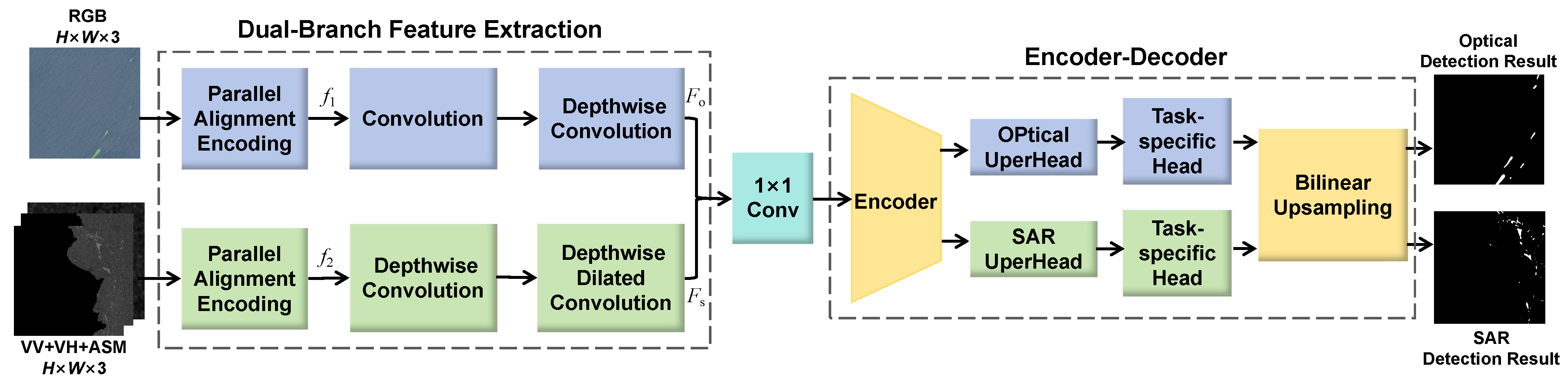
To address the aforementioned limitations of existing methods, we develop a novel multimodal framework named DMDNet for Ulva prolifera detection, aiming to build a universal all-in-one model that efficiently processes heterogeneous optical and SAR remote sensing data. Distinct from conventional multimodal algorithms, DMDNet performs multimodal joint training using unpaired optical and SAR samples rather than direct multimodal feature fusion. During inference, the two modalities are processed independently to achieve accurate Ulva prolifera detection on both types of data. The main contributions of this work are summarized as follows:

1.

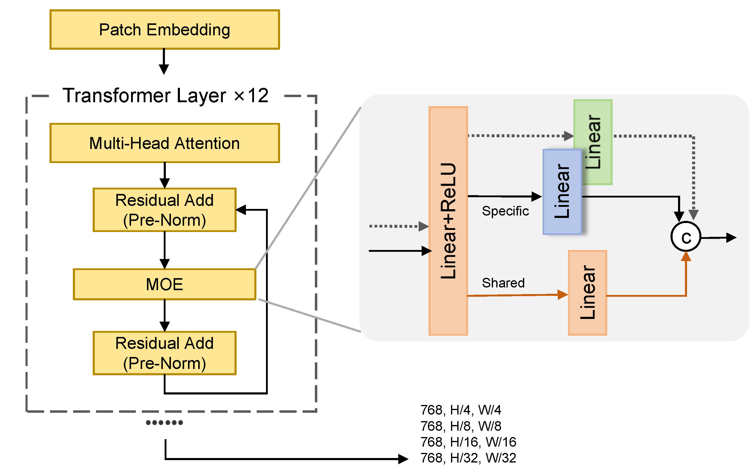
We integrate the Mixture of Experts (MoE) mechanism into the encoder–decoder module. Specifically, the shared branch in MoE extracts universal features of Ulva prolifera, while the modality-specific expert branches acquire modal differences. This mechanism makes the encoder adaptively select proper expert branches according to varied spatial characteristics in optical and SAR data, effectively enhancing feature representation for complex marine scenes.

2.

We propose a multimodal joint training strategy. In each iteration, optical and SAR image samples are fed into the network simultaneously. Both modalities share the same ViT backbone for feature extraction and generate segmentation results via task-specific expert branches and decoding heads. The training losses calculated from the two samples are backpropagated jointly to update the parameters of the shared backbone synchronously.

3.

We design a multimodal composite loss function. The cross-entropy (CE) loss alleviates class imbalance and overfitting. The region consistency loss guides the model toward tiny algal targets and boundaries via edge-aware weighting. The boundary consistency loss sharpens segmentation outlines by enforcing gradient consistency between predictions and ground truth.

2. Decoupled Multimodal Ulva Prolifera Detection

2.1. DMDNet

The main architecture of the proposed DMDNet is illustrated in Figure 1. The network accepts two types of inputs: RGB optical images and three-channel SAR data composed of VV, VH, and ASM components. Both inputs have a dimension of $H\times W\times 3$. First, a dual-branch feature extraction module equipped with parallel alignment encoding structures is utilized to extract modality-specific features for the two data types separately. The two streams of modal features pass through a $1\times 1$ convolutional layer for dimension normalization. The unified features are fed into the pre-trained ViT-B/MoE [35] encoder to mine deep semantic representations. Two independent task-specific decoders are configured for the optical and SAR modalities, each followed by a task-specific head that maps the refined features to a pixel-wise class probability space. Finally, bilinear upsampling is adopted to restore the original resolution of feature maps, and binary segmentation masks of Ulva prolifera corresponding to optical and SAR inputs are generated separately.

2.1.1. Dual-Branch Feature Extraction

This module is designed to alleviate the heterogeneity of feature distributions between optical and SAR images. During the parallel alignment encoding, inputs of the two modalities are processed separately by basic $3\times 3$ convolution blocks, which map heterogeneous data into a unified shallow feature space and facilitate subsequent deep feature learning. The unified features are then fed into two parallel branches with distinct convolutional architectures to adaptively capture modality-specific characteristic features. Specifically, the optical branch combines standard $3\times 3$ convolution and depthwise separable convolution to preserve fine spectral and texture details and strengthen the features of tiny Ulva prolifera patches. The SAR branch adopts $3\times 3$ depthwise separable convolution together with dilated convolution to expand the model’s receptive field, suppress speckle noise in images, and effectively improve the feature separability between Ulva prolifera and seawater background. The two branches are described as follows:

$$F_{\mathrm{o}}={\varphi }_{\mathrm{o}}\left(f_1\right),F_{\mathrm{s}}={\varphi }_{\mathrm{s}}\left(f_2\right),$$

(1)

where $f_1$ and $f_2$ represent the input features separately. ${\varphi }_{\mathrm{o}}(·)$ and ${\varphi }_{\mathrm{s}}(·)$ denote the affine mapping functions for optical and SAR branches; $F_{\mathrm{o}}$ and $F_{\mathrm{s}}$ denote the modality-specific features.

2.1.2. Encoder–Decoder

Due to the differences in imaging mechanisms between optical and SAR remote sensing images, directly feeding raw heterogeneous data into the network tends to cause feature entanglement. In this case, the model cannot effectively distinguish the inherent semantic information of Ulva prolifera from modal noise and unique textures introduced by different sensors. To address this issue, an MoE [36] block is introduced into the feed-forward network of ViT-B to replace the traditional single shared feed-forward network (FFN). The overall structure of the ViT-B/MoE encoder is shown in Figure 2. The multimodal feature space is decomposed into two mutually uncoupled subspaces—modality-agnostic common features and modality-specific personalized features—which are independently modeled by the shared branches and modality-specific expert branches, respectively. This design mitigates feature conflicts between the two data sources at the source end. Specifically, after being pre-trained on the RS4P-1M [35] remote sensing dataset, the encoder’s shared branch gains the capability to extract general remote sensing features. In the joint training phase, this branch further learns shared semantic features common to both optical and SAR images. By contrast, one expert is assigned for each dataset task; the expert branches separately learn modality-adaptive exclusive representations for different modalities. This design retains modality-specific information while sharing universal features to adapt to the domain discrepancies between optical and SAR data.

Let $h^{\left(l\right)}\in {\mathbb{R}}^{N\times C}$ denote the input token feature of the l-th layer of the Transformer, where N is the token sequence length and C is the feature channel number. First, nonlinear transformation of the input features is performed through the shared branch to learn multimodal generic semantic features:

$$z_{\mathrm{shared}}^{\left(l\right)}=f_{\mathrm{s}}^{\left(l\right)}\left(h^{\left(l\right)}\right)\in {\mathbb{R}}^{N\times (C-p)},$$

(2)

where p denotes the number of expert branch channels; $f_{\mathrm{s}}^{\left(l\right)}$ denotes the nonlinear mapping function belonging to the shared branch in the l-th layer.

Then, according to the dataset identifier d of the current sample, the corresponding expert is selected by the task mapping function $e(·)$, obtaining specific features:

$$z_{\mathrm{specific}}^{\left(l\right)}=f_{\mathrm{e}(d)}^{\left(l\right)}\left(h^{\left(l\right)}\right)\in {\mathbb{R}}^{N\times p}.$$

(3)

where $f_{\mathrm{e}(d)}^{\left(l\right)}$ refers to the nonlinear mapping function of the d-modality-specific expert branch in the l-th Transformer layer.

The two features are concatenated along the channel dimension to form the output of the MoE block:

$${\tilde{h}}^{\left(l\right)}=\mathrm{Concat}\left(z_{\mathrm{shared}}^{\left(l\right)},z_{\mathrm{specific}}^{\left(l\right)}\right).$$

(4)

Finally, the update is completed via residual connection:

$$h^{(l+1)}=h^{\left(l\right)}+{\tilde{h}}^{\left(l\right)}.$$

(5)

We remove the class token from the selected Transformer layers and reshape token sequences into spatial feature maps [B, C, H, W]. A lightweight FPN module generates four feature branches with resolutions of $H/4\times W/4$, $H/8\times W/8$, $H/16\times W/16$, and $H/32\times W/32$ via transposed convolution, identity mapping, and max-pooling operations, which are subsequently fed into the decoder. The decoder consists of an UPerHead [37] module and task-specific classification heads, and its detailed architecture is illustrated in Figure 3.

The three shallower feature maps at resolutions of $H/4\times W/4$, $H/8\times W/8$, and $H/16\times W/16$ first undergo independent $1\times 1$ convolutions to uniformly compress the number of channels to 256. The deepest feature map with a resolution of $H/32\times W/32$ is delivered to the pyramid pooling module (PPM) [38]. The PPM contains four parallel adaptive average pooling branches with pooling scales of $1\times 1$, $2\times 2$, $3\times 3$, and $6\times 6$, respectively. After pooling, each branch adopts a $1\times 1$ convolution for channel dimension reduction followed by bilinear upsampling to restore the original feature resolution. Afterwards, the four pooled feature streams are concatenated with the original deep features, and a $3\times 3$ convolution layer is applied for feature refinement. The refined deep features are then fused with shallow features layer by layer from deep to shallow via upsampling element-wise addition, integrating global deep semantic information into fine-grained shallow spatial details. All fused multi-level features are upsampled to the resolution of $H/4\times W/4$ and concatenated together, then further optimized through a single $3\times 3$ convolution layer. Finally, the task-specific head outputs pixel-wise segmentation predictions.

2.2. Loss Function

To enhance the discriminability of the Ulva prolifera main regions and boundaries in multimodal joint segmentation, a task-weighted comprehensive loss function is designed. Through a three-tier mechanism incorporating class imbalance adaptation, target region enhancement, and boundary consistency constraint, precise optimization tailored to the Ulva prolifera segmentation task is achieved.

For a single-modality dataset d, its loss function consists of basic segmentation loss and a spatial attention constraint, formulated as follows:

$$L_d=L_{\mathrm{CE}}^{\left(d\right)}+{\alpha }_d{L}_{\mathrm{att}}^{\left(d\right)},$$

(6)

where $L_{\mathrm{CE}}^{\left(d\right)}$ denotes CE loss with class reweighting, $L_{\mathrm{att}}^{\left(d\right)}$ represents the spatial attention constraint loss, and ${\alpha }_d$ is the spatial attention constraint loss coefficient. ${\alpha }_d$ is scheduled piecewise as $0.05\to 0.20\to 0.10$ for SAR data and ${\alpha }_d=0.08$ for optical data.

2.2.1. Cross-Entropy Loss with Class Reweighting

To mitigate foreground–background distribution imbalance in remote sensing segmentation, class weights are incorporated into the CE loss to assign larger penalty coefficients to target classes [39]. This improves the model’s focus on minority foreground regions and is defined as

$$L_{\mathrm{CE}}^{\left(d\right)}=-{\displaystyle \frac{1}{N}}{\displaystyle \sum _{i=1}^N}{\omega }_{g_i}^{\left(d\right)}log{p}_{i,g_i}^{\left(d\right)},$$

(7)

where d denotes the current dataset, N represents the total number of pixels, $g_i$ is the ground truth label of the i-th pixel, $p_{i,g_i}^{\left(d\right)}$ is the model’s predicted probability for the ground truth class, and ${\omega }_{g_i}^{\left(d\right)}$ denotes the corresponding class weight.

2.2.2. Spatial Attention Constraint Loss

The spatial attention constraint loss is further split into region consistency loss and boundary consistency loss, which regularize the integrity of segmented regions and boundaries, respectively. It is defined as

$$L_{\mathrm{att}}=L_{\mathrm{reg}}+{\lambda }_b{L}_{\mathrm{bnd}},$$

(8)

where ${\lambda }_b$ denotes the weighting coefficient for boundary consistency loss. The weights are 0.10 for SAR and 0.25 for FIO-EP.

The region consistency loss $L_{\mathrm{reg}}$ regularizes spatial distribution consistency between Ulva prolifera segmentation outputs and ground truth binary masks. Edge weights and small-target enhancement weights are introduced to emphasize the learning of Ulva prolifera boundaries and fine fragmented patches. It is given by

$$L_{\mathrm{reg}}={\displaystyle \frac{1}{N}}{\displaystyle \sum _{i=1}^N}{W}_{\mathrm{edge}}·W_{\mathrm{small}}·|\mathcal{P}-Y|,$$

(9)

where $\mathcal{P}$ denotes the model prediction, and Y denotes the corresponding ground truth binary map. The edge weight is defined as $W_{\mathrm{edge}}=1+\parallel \nabla Y_i\parallel$, where ∇ stands for the Sobel gradient operator. The small-target enhancement weight is $W_{\mathrm{small}}=1+\beta exp\left(-{\displaystyle \frac{r}{\tau +ϵ}}\right)$, in which r denotes the target area ratio, and $\beta$ and $\tau$ are empirical hyperparameters, where $\beta =0.7$, $\tau =0.05$, and $ϵ={10}^{-6}$.

The boundary consistency loss $L_{\mathrm{bnd}}$ employs the normalized Charbonnier loss [40] to enforce gradient consistency on boundaries between model outputs and ground truth maps. It is formulated as

$$L_{\mathrm{bnd}}={\displaystyle \frac{1}{N}}\sum {\displaystyle \frac{\sqrt{{(\nabla P-\nabla Y)}^2+ϵ}}{\mathrm{mean}\left(\parallel \nabla Y\parallel +ϵ\right)}},$$

(10)

where N denotes the total number of pixels, $\nabla P$ and $\nabla Y$ represent gradients of the prediction and ground truth label, respectively, and $ϵ$ is a smoothing constant to prevent division by zero.

Ultimately, the overall loss is expressed as

$$L=\sum _{d\in D}{w}_d{L}_d,$$

(11)

where D denotes the set of modalities used for joint training, and $w_d$ is the modality-wise task weight. In experiments, $w_d=0.65$ for CODC-SAR and $w_d=0.35$ for FIO-EP.

2.3. Training and Test Procedures

This paper proposes a multimodal joint training strategy. During training, optical and SAR image samples are fed into the network simultaneously at each iteration. Both modalities share the identical ViT backbone for feature extraction and generate segmentation outputs separately via modality-specific expert branches and decoder heads. The loss functions of the two modalities are backpropagated jointly to synchronously optimize the parameters of the shared ViT backbone. Under this training paradigm, the shared ViT obtains gradient signals from both optical and SAR modalities at each optimization step. This enables the network to learn discriminative universal multimodal features suitable for heterogeneous remote sensing data. Furthermore, the expert branches and decoder heads isolate modality-specific intrinsic biases. While learning shared universal representations, the model is capable of preserving discriminative characteristics unique to each individual modality.

Taking the joint training on the FIO-EP and CODC-SAR datasets as an instance, the detailed pipeline of the multimodal training phase is illustrated in Algorithm 1.

Algorithm 1: Multimodal Training and Test Procedures of DMDNet

Input: Optical dataset $D_{\mathrm{o}}$ and SAR dataset $D_{\mathrm{s}}$ with pixel-wise binary    segmentation masks; Output: Trained parameters of the DMDNet model. Initialize network parameters of DMDNet for each training epoch do  for each batch sampled from all tasks via zip do   for each task $t\in \{\mathrm{FIO}-\mathrm{EP},\mathrm{CODC}-\mathrm{SAR}\}$ do    Load image $I_t$ and mask $Y_t$ from corresponding dataloader    if $t=\mathrm{SAR}$ then     Unify SAR features according to Equation (1);    else     Unify optical features according to Equation (1);    end    Project features to three-channel representation via $1\times 1$ convolution on     the aligned features;    Extract multi-scale features via shared ViT backbone;    Decode via task-specific UPerHead;    Generate segmentation prediction;    Compute composite loss according to Equation (8);   end   Compute total loss according to Equation (11);   Perform single backpropagation step to update all parameters;  end end Test phase: Disable gradient computation and Dropout; Perform single-modality independent inference on each test sample.

Specifically, let the optical sample be $(x_{\mathrm{o}},y_{\mathrm{o}})$ and the SAR sample be $(x_{\mathrm{s}},y_{\mathrm{s}})$. The two modalities share ViT parameters denoted as ${\theta }_{\mathrm{share}}$. The parameter set of the optical expert branch is ${\theta }_{\exp }^{\mathrm{o}}$, and the parameter set of the SAR expert branch is ${\theta }_{\exp }^{\mathrm{s}}$. The optimization objective at each training step is formulated as

$$\begin{array}{cc}\hfill \mathcal{L}& =w_{\mathrm{o}}·{\mathcal{L}}_{\mathrm{ce}}\left(f(x_{\mathrm{o}};{\theta }_{\mathrm{share}},{\theta }_{\exp }^{\mathrm{o}}),y_{\mathrm{o}}\right)\hfill \\ \hfill & +w_{\mathrm{s}}·{\mathcal{L}}_{\mathrm{ce}}\left(f(x_{\mathrm{s}};{\theta }_{\mathrm{share}},{\theta }_{\exp }^{\mathrm{s}}),y_{\mathrm{s}}\right)\hfill \end{array}$$

(12)

where $w_{\mathrm{o}}$ and $w_{\mathrm{s}}$ represent the weight coefficients for the two segmentation tasks.

When calculating the gradient ${\nabla }_{{\theta }_{\mathrm{share}}}\mathcal{L}$ with respect to the shared parameters ${\theta }_{\mathrm{share}}$, gradient signals are aggregated from both the optical and SAR modalities. This mechanism constrains the shared feature space to produce robust activations toward Ulva prolifera targets in both types of remote sensing imagery. In contrast, the gradients ${\nabla }_{{\theta }_{\exp }^{\mathrm{o}}}\mathcal{L}$ for the optical expert branch and ${\nabla }_{{\theta }_{\exp }^{\mathrm{s}}}\mathcal{L}$ for the SAR expert branch are mutually independent. Each modality-specific expert branch is optimized individually to accommodate the inherent distribution shift exclusive to its corresponding data modality.

3. Experiments

3.1. Dataset

3.1.1. FIO-EP Dataset

The optical dataset adopted in our experiments is the FIO-EP dataset [41]. The image samples of the FIO-EP dataset are collected from the Yellow Sea of China, covering coastal waters from the Subei Shoal to the offshore areas along the Shandong Peninsula. This dataset integrates true-color images captured by domestic high-resolution satellites including GF-1, GF-2, and ZY3-02. Samples are collected hierarchically based on three core interference factors that affect the detection accuracy of Ulva prolifera, namely radiance difference, floating macroalgae distribution patterns, and cloud coverage levels. It fully covers the entire life cycle of green tide algae, including germination, outbreak and recession, as well as realistic complex observation conditions such as cloudy weather, low illumination, and strong sunlight. The dataset consists of 1334 annotated image patches with a uniform resolution of $512\times 512$ pixels, where binary black-and-white masks are utilized to distinguish the seawater background and Ulva prolifera foreground. We split the whole dataset into training, validation, and test subsets at a ratio of 3:1:1. Notably, we follow the official 3:1:1 scene-level split of the FIO-EP dataset. Each sample is one independent high-resolution scene image; the three subsets are strictly disjoint at the scene level, and no image patch appears in more than one subset. In all experiments, the original image patches are directly fed into the model without extra cropping operations.

3.1.2. The Green Tide Coverage Product in the Yellow Sea During 2008–2022

The data used in experiments is provided by the Oceanographic Data Center, Chinese Academy of Sciences (CODC) [42]. This dataset is divided into two subsets: the optical green tide annotation subset and the SAR green tide annotation subset. All samples are stored in PNG format and split into training and test sets archived in separate folders according to different observation periods. All annotated samples from various periods can be integrated for joint model training.

The optical subset is constructed from MODIS imagery collected from 9 May to 15 July 2019, with a spatial resolution of 500 m and seven spectral bands. Band 1 (red), Band 4 (green), and Band 3 (blue) are combined to generate RGB images. Original $128\times 128$ pixel patches are resized to $512\times 512$ pixels during training. This resizing operation only adjusts the network input size and cannot improve the actual spatial resolution of the original imagery. Binary segmentation masks are matched accordingly, where pixel value 0 refers to the seawater background and 1 corresponds to the Ulva prolifera foreground. The dataset is partitioned into 1126 training samples, 198 validation samples, and 662 test samples. Although the training and validation sets cover the same time span, their image patches are spatially disjoint. In contrast, the test set exclusively adopts images from completely new temporal periods that are not involved in the training and validation phases.

The SAR subset is derived from Sentinel-1 SAR imagery acquired from 2015 to 2019, with $256\times 256$-pixel samples at 30 m spatial resolution. It contains five channels including VV polarization, VH polarization, as well as ASM, entropy, and mean texture features extracted via the gray level co-occurrence matrix (GLCM). Three-channel feature maps are composited using VV, VH, and ASM, resized to $512\times 512$ pixels and saved as 8-bit grayscale PNG. Original label pixels are defined as 0 for background and 255 for green tide targets, which are remapped to binary labels 0 and 1 in the preprocessing pipeline. The dataset is split into 943 training samples, 104 validation samples, and 104 test samples. The original annotated samples are stored in training- and test-related folders according to different annotation periods, and no independent validation set is provided in the official release. We construct the validation set from the official training samples. Although the acquisition dates of validation and test samples may partially overlap with those of training samples, their sampled geographic regions are completely non-overlapping with the training set. All patches originating from the same geographic region are assigned to only one subset, preventing geographically adjacent patches from being distributed across different data partitions.

3.2. Experimental Settings

All experiments are implemented based on PyTorch 2.3.1, and the training and inference are completed on a single NVIDIA RTX 3090 GPU. The AdamW optimizer is adopted with an initial learning rate set to $1\times {10}^{-4}$ and weight decay set to 0.05. A cosine annealing learning rate scheduler is used, with linear warm-up applied for the first 5 epochs. The two datasets are jointly trained for 100 epochs, with an input crop size of $512\times 512$ pixels and a batch size of 2. All datasets are modeled as binary classification tasks (foreground/background). Each task has its own DataLoader with a DistributedSampler. To balance training across tasks, all datasets are replicated to the maximum dataset length so that each epoch contains an identical number of samples per task, and batches are paired via zip across loaders. Class weights are manually set as fixed coefficients rather than frequency-based statistics. For the binary tasks, the foreground weight is base 3.0 scaled by a per-task-capped factor: (1.0, 6.0) for CODC-SAR/optical and (1.0, 7.5) for FIO-EP. We adopt a unified data augmentation pipeline for all experimental data, including random cropping, flipping, 90° rotation, color jitter, grayscale transformation, and Gaussian blur. For SAR data, we additionally apply gamma jitter and multiplicative speckle noise. In our experiments, average accuracy (aAcc), mean intersection over union (mIoU), mean F1-score (mF1), mean precision (mPrecision), and mean recall (mRecall) are selected as the evaluation metrics to comprehensively assess the segmentation performance of the proposed model on the different datasets. We conduct repeated experiments with three random seeds (24, 1156, 123) for core model configurations and ablation groups. For each run, we select the checkpoint achieving the best mIoU on the validation set and perform one-shot evaluation on the fixed test set. The values reported in all tables are the best results obtained from these three independent trials.

3.3. Performance Comparison

To verify the segmentation performance of the proposed method, we conduct quantitative comparisons with several state-of-the-art semantic segmentation models, including SegNet [43], U-Net [44], DeepLabV3+ [45], ResUnet-a [46], SegNeXt [47], LCS-Net [48], and GLANet [49]. The quantitative results of all models on the FIO-EP dataset under identical experimental conditions are shown in

Table 1. Quantitative comparison results on the FIO-EP dataset.

	aAcc	mIoU	mF1	mPrecision	mRecall
SegNet	0.9878	0.8546	0.9160	0.9577	0.8819
U-Net	0.9884	0.8632	0.9217	0.9538	0.8942
DeeplabV3+	0.9896	0.8773	0.9308	0.9540	0.9101
ResUnet-a	0.9900	0.8798	0.9324	0.9645	0.9048
SegNeXt	0.9888	0.8653	0.9231	0.9625	0.8903
LCS-Net	0.9796	0.7981	0.8763	0.8614	0.8927
GLANet	0.9915	0.8983	0.9439	0.9626	0.9268
Ours	0.9894	0.8876	0.9374	0.9102	0.9690

The best-performing value in each column is marked in bold.

. It reports the evaluation results of the proposed DMDNet model jointly trained with multimodal data and tested on the FIO-EP dataset. The best values are marked in bold.

The DMDNet model achieves the best performance on mRecall on the FIO-EP dataset, as shown in Table 1. Compared with the best-performing baseline GLANet, our model yields a 1.2% drop in mIoU and a slight decrease of 0.7% in mF1, yet achieves a 4.4% improvement in mRecall. This demonstrates that our method possesses strong recognition capability for fragmented nearshore Ulva prolifera patches and effectively reduces target omission. Among all competitors, ResUnet-a achieves the highest mPrecision, whereas our proposed model outperforms only LCS-Net in terms of mPrecision. Such a performance gap reveals the well-known precision–recall trade-off in green tide segmentation: high-performance baselines tend to generate conservative predictions to suppress false detections, at the cost of detection completeness for scattered small-scale algae regions. Combined with the results in

Table 2. Quantitative comparison results on the CODC-optical dataset.

	aAcc	mIoU	mF1	mPrecision	mRecall
SegNet	0.9794	0.5325	0.5736	0.7492	0.5456
U-Net	0.9796	0.5616	0.6204	0.7517	0.5811
DeeplabV3+	0.9799	0.5206	0.5527	0.8061	0.5314
ResUnet-a	0.9780	0.5659	0.6278	0.7056	0.5942
SegNeXt	0.9750	0.5470	0.6001	0.7216	0.5671
LCS-Net	0.9435	0.4938	0.5278	0.5224	0.5435
GLANet	0.9781	0.5217	0.5558	0.6676	0.5357
Ours	0.9771	0.6161	0.6975	0.7123	0.6847

The best-performing value in each column is marked in bold.

, it can be observed that although GLANet achieves competitive performance on the FIO-EP dataset, its accuracy degrades below our model on the more challenging CODC-optical dataset, which verifies the superior cross-scene generalization ability of our approach. The aAcc values of all models range from 0.9796 to 0.9915. Affected by the large proportion of seawater background pixels, this metric exhibits low discriminative power and can only serve as an auxiliary reference. In summary, compared with single-modal networks, our method greatly improves the integrity of segmentation maps, showing prominent advantages in extracting fine-grained algae patches and reducing missed detections, which confirms its suitability for high-precision Ulva prolifera monitoring.

To further verify the segmentation capability of the proposed optical-SAR joint training model for optical Ulva prolifera imagery, comparative experiments are carried out on the CODC-optical dataset with RGB three-band composite input, and the quantitative results are listed in Table 2. Compared with the FIO-EP dataset, the CODC-optical scenes contain more complex nearshore coastal backgrounds, leading to generally degraded performance for all competing models. The proposed model achieves optimal values for three core metrics, namely mIoU, mF1, and mRecall. It obtains an mIoU of 0.6161, which is prominently higher than all competing models and indicates the highest consistency between predicted Ulva prolifera regions and ground truth labels. The mF1 of 0.6975 achieves a balanced trade-off between false positives and missed detections, while the high mRecall of 0.6847 effectively mitigates the omission of scattered Ulva prolifera patches across extensive offshore waters. Notably, our model maintains the high-recall property observed on the FIO-EP dataset. This stable tendency demonstrates that the multimodal joint training enables our network to prioritize capturing scattered Ulva prolifera patches under diverse optical coastal conditions. In summary, the proposed model still outperforms various unimodal semantic segmentation networks on this optical dataset, presenting distinct advantages in improving the integrity of Ulva prolifera segmentation and reducing target missing detection.

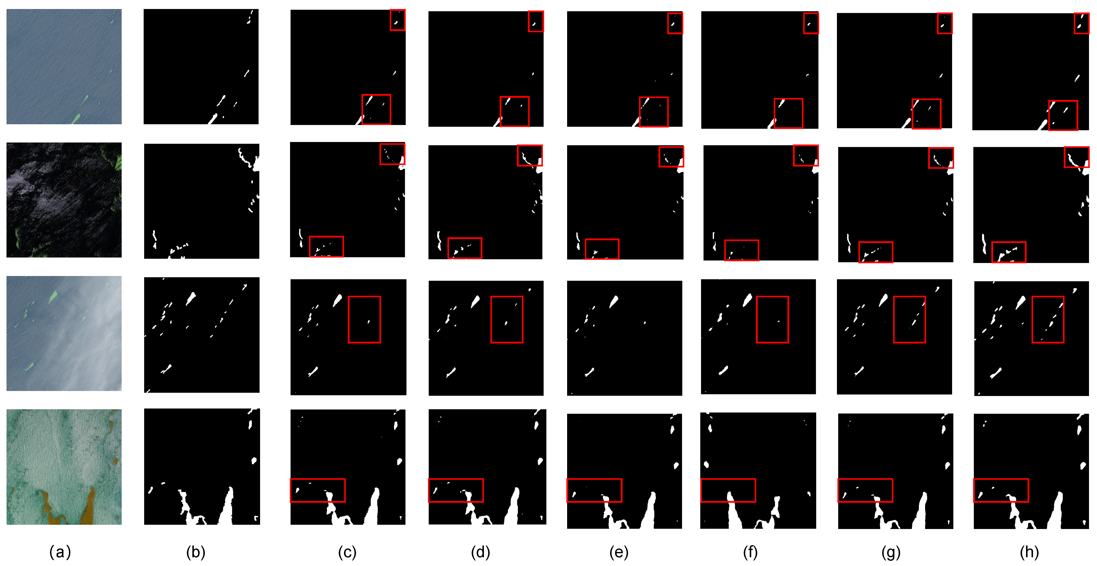
Figure 4 presents visual segmentation comparisons of different models for Ulva prolifera extraction on the FIO-EP dataset, with Ulva prolifera samples from four typical observation scenarios selected for qualitative evaluation. As indicated by the prediction maps, ResUnet-a and SegNeXt cannot fully segment fragmented tiny algae patches and suffer prominent missed detections. Although U-Net and DeepLabV3+ can identify most algal areas, they generate coarse segmentation edges, accompanied by frequent contour fracture and omission of micro-scale algae spots. Although GLANet achieves the optimal mIoU on the FIO-EP dataset, it is still prone to missing Ulva prolifera patches under complex interferences such as cloud cover, while our method successfully identifies these obscured target regions. The proposed optical-SAR joint training model exploits complementary characteristics of multi-source remote sensing data. It accurately reconstructs intact boundaries of fragmented Ulva prolifera inside the red-boxed regions, greatly alleviating missed detections and generating segmentation contours that are more consistent with the ground truth, while restraining false segmentation triggered by seawater clutter. This visual evidence intuitively demonstrates the superiority of the proposed method in refined extraction of scattered nearshore Ulva prolifera and corroborates the conclusions obtained from the previous quantitative metric analysis.

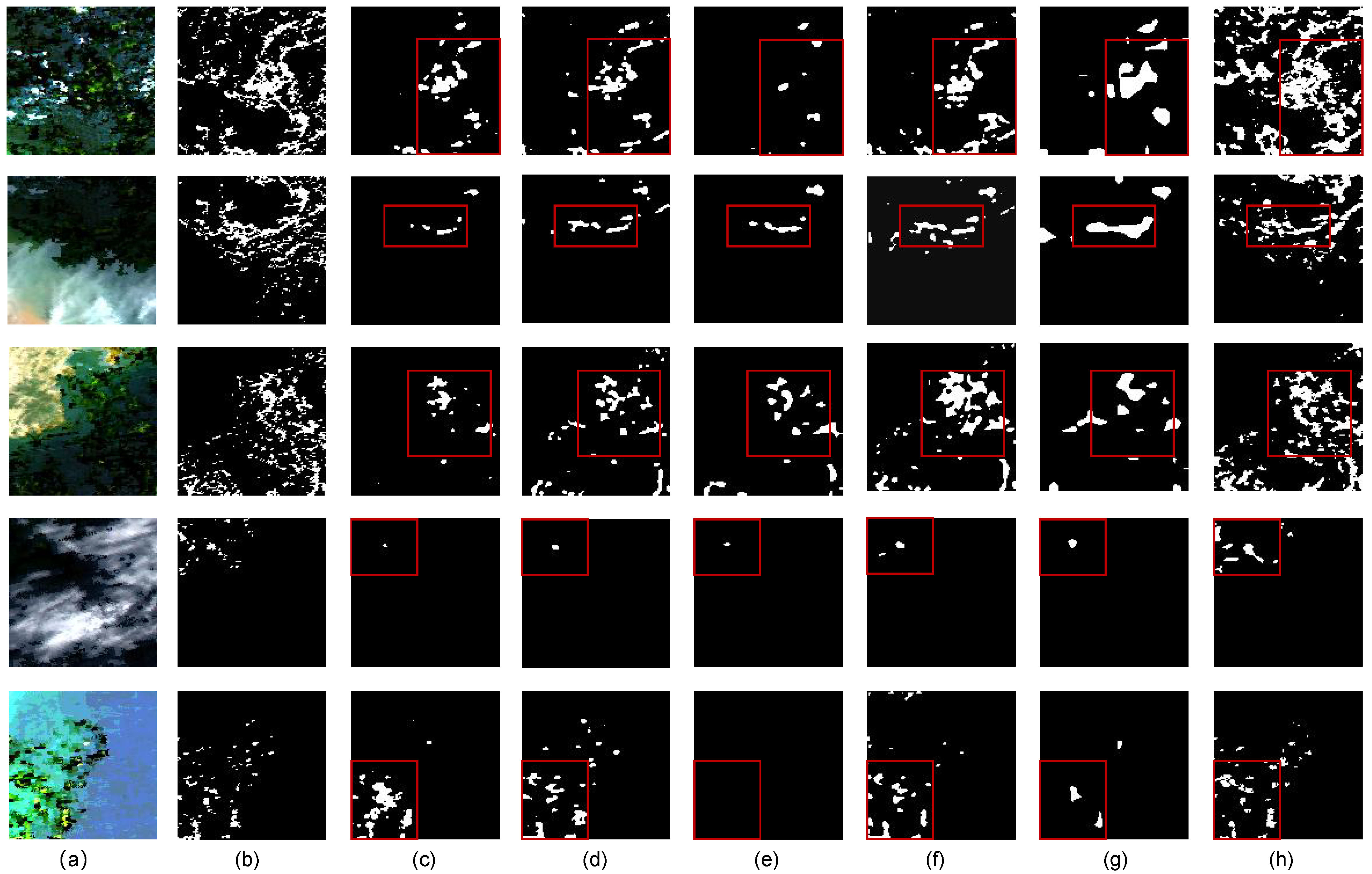
Figure 5 shows qualitative segmentation comparisons of different models on the CODC-optical dataset with five groups of typical marine samples. As can be observed from the segmentation outputs of baseline methods, SegNet, DeepLabV3+, and SegNeXt perform poorly in detecting small and scattered Ulva prolifera patches, generating foreground regions far smaller than the ground truth, and suffering from severe missed detections. ResUnet-a and U-Net are able to capture the main algae bodies, whereas numerous tiny patches and fine algae edges are lost, resulting in incomplete segmentation contours. Especially for the fourth sample affected by cloud interference, all baselines can only extract a tiny number of algae pixels, indicating evident segmentation degradation. The segmentation results of the proposed DMDNet model achieve a higher degree of consistency with the ground truth and effectively suppress false detections caused by sea clutter and cloud noise. Our method surpasses all comparative baselines under various complex scenarios, which visually demonstrates the performance improvement in the DMDNet model for Ulva prolifera segmentation.

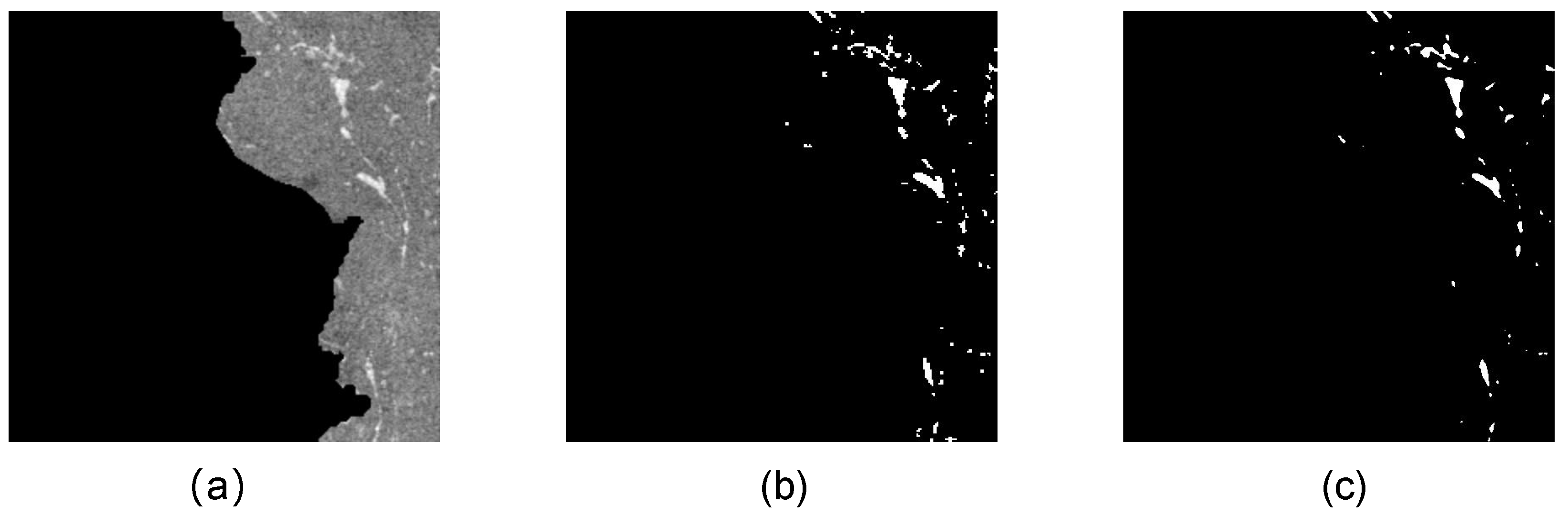
Figure 6 presents the visual segmentation results of the proposed model on the SAR dataset. By comparison, the proposed optical-SAR joint training method can accurately extract target Ulva prolifera regions from SAR imagery, with segmentation contours in good agreement with the ground truth. The model effectively identifies scattered algal patches distributed along the coastline, which verifies that our method achieves reliable green tide segmentation performance when taking SAR data as individual input.

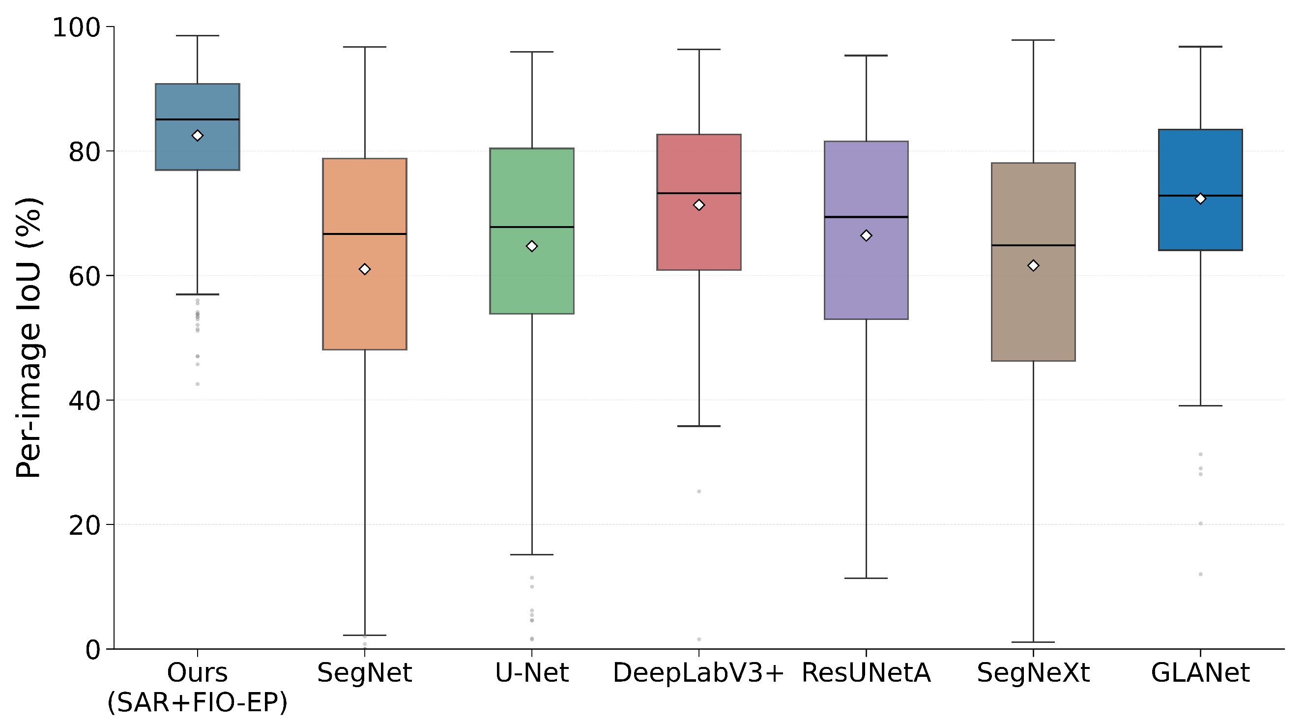
As shown in Figure 7, the box-whisker plot illustrates the per-image IoU distribution across all test samples. Our method achieves the highest median IoU with the narrowest inter-quartile range, demonstrating low performance fluctuation on diverse test images. By contrast, most baseline models produce numerous outlier samples with extremely low IoU values, indicating segmentation failure under challenging conditions such as cloud-obscured scenes and fragmented algae patches. Even GLANet, which achieves competitive overall mIoU, suffers from obvious accuracy degradation on several difficult samples. These statistical results further verify that our cross-modal training strategy greatly improves prediction stability and adaptability to complex marine observation scenarios.

In summary, the proposed method achieves outstanding performance in mRecall, while obtaining competitive results for mIoU, mF1, mPrecision, and aAcc. These findings validate the effectiveness and superiority of our approach for green tide segmentation, enabling more precise and complete extraction of Ulva prolifera target regions.

3.4. Ablation Studies

To verify the effectiveness of each core design component, ablation experiments on the MoE module and the improved loss function are conducted under identical training configurations. Two comparative strategies are set accordingly: replacing the MoE module with the standard ViT and substituting the comprehensive loss function with CE loss. The experimental results are presented in

Table 3. Ablation study on MoE and loss function.

MoE	Loss	mIoU		Average mIoU
		FIO-EP	CODC-SAR
		0.8848	0.6722	0.7785
	✓	0.8925	0.6577	0.7752
✓		0.8818	0.6599	0.7709
✓	✓	0.8876	0.7546	0.8211

The best-performing value in each column is marked in bold.

. The complete model achieves an mIoU of 0.8876 on the FIO-EP dataset and 0.7546 on the CODC-SAR dataset, with an average mIoU of 0.8211 and the best overall performance.

When only the comprehensive loss function or only the MoE module is activated, no overall performance improvement is observed, and slight accuracy degradation even occurs in the average mIoU. This indicates that a single component alone cannot bridge the large domain gap between optical and SAR modalities. By contrast, when both the MoE encoder and comprehensive loss function are enabled, the average mIoU of the full model increases by 5.5% compared with the baseline model without these two core designs. Both FIO-EP and CODC-SAR obtain performance gains to varying degrees. The performance improvement is mainly reflected in the more challenging SAR modality, where the mIoU is increased by 12.3%. These results demonstrate the remarkable cooperative effect between the MoE module and comprehensive loss function. The expert-routing mechanism of MoE captures modality-specific divergent features, while the comprehensive loss function constrains multimodal joint optimization. Only the combination of the MoE encoder and the comprehensive loss function can effectively alleviate the domain discrepancy between optical and SAR modalities, thereby improving the segmentation performance of multimodal samples. To explore the individual contributions of spatial attention constraint loss and boundary consistency loss within the comprehensive loss function, ablation experiments are carried out with other modules fixed. The model adopting only standard CE loss is regarded as the baseline, and the experimental results are summarized in

Table 4. Ablation study on loss function.

Loss		mIoU		Average mIoU
${\mathit{L}}_{\mathrm{att}}$	${\mathit{L}}_{\mathrm{bnd}}$	FIO-EP	CODC-SAR
		0.8785	0.7046	0.7916
✓		0.8808	0.7013	0.7911
✓	✓	0.8876	0.7546	0.8211

The best-performing value in each column is marked in bold.

. For the baseline model with CE loss, the mIoU reaches 0.8785 and 0.7046 on the FIO-EP and CODC-SAR datasets, respectively, with an average mIoU of 0.7916. When only the spatial attention constraint loss is introduced without boundary consistency loss, only marginal improvement can be observed on the optical FIO-EP dataset, while the SAR modality obtains nearly no performance gain, and the overall performance remains comparable to the baseline. This indicates that the spatial attention constraint loss alone cannot tackle the segmentation difficulties caused by heavy noise and blurred object boundaries in SAR images. After integrating both spatial attention constraint loss and boundary consistency loss to form the full composite loss function, the average mIoU increases by 3.7% compared with the baseline. Specifically, the mIoU of the SAR dataset is improved by 7.1%, and the mIoU of the FIO-EP dataset increases by 1.0%. These results demonstrate the synergistic effect between spatial attention constraint loss and boundary consistency loss. The spatial attention constraint loss drives the model to focus on Ulva prolifera target regions, and the boundary consistency loss is dedicated to optimizing blurred object contours in images. Joint constraints from the two loss terms effectively refine edge segmentation for SAR samples and improve the overall multimodal segmentation performance.

To investigate the effect of different dataset matching strategies on the segmentation accuracy of the proposed DMDNet model, two ablation experiments involving cross-dataset and same-dataset joint training are conducted. The mIoU values on the optical subset, SAR subset, and the corresponding average mIoU of the two configurations are summarized in

Table 5. Ablation study on different dataset matching strategies.

Dataset Matching Strategy	mIoU		Average mIoU
	FIO-EP	CODC-SAR
FIO-EP + CODC-SAR	0.8876	0.7546	0.8211
CODC-optical + CODC-SAR	0.6161	0.5291	0.5726

.

When the model is jointly trained with FIO-EP optical data and CODC-SAR data, it achieves mIoU values of 0.8876 and 0.7546 on the optical and SAR test sets, respectively, with an average mIoU of 0.8211. In contrast, the joint training scheme using CODC-optical and CODC-SAR data yields a performance decline. Specifically, the optical and SAR mIoU are decreased by 30.6% and 29.9%, respectively, and the average mIoU is decreased by 30.3%. Notably, the significant performance gap between the two schemes cannot be simply attributed to the dataset matching strategy. Instead, it is largely determined by inherent differences in data quality and spatial resolution. The FIO-EP dataset consists of high-resolution Gaofen satellite optical images with abundant spatial details and distinguishable texture features. In comparison, the CODC-optical subset is derived from 500-meter-resolution MODIS imagery. After upsampling the original $128\times 128$ patches to $512\times 512$, the CODC-optical images retain limited valid spatial information and contain severe background noise, resulting in an inherently low segmentation baseline. The comparison indicates that high-quality FIO-EP samples provide richer fine-grained features and more reliable feature priors for multimodal training, enabling the model to better exploit the features from optical and SAR information. Therefore, the performance advantage of the dataset matching strategies mainly demonstrates the superiority of high-resolution optical data in multimodal segmentation tasks, rather than proving that cross-dataset joint training is inherently better than same-dataset joint training.

To fully verify the effectiveness of the proposed joint training strategy, we carry out ablation comparative experiments as presented in

Table 6. Ablation study on joint training strategy.

Training Strategy	mIoU		Average mIoU
	FIO-EP	CODC-SAR
Only FIO-EP	0.8984	0.0880	0.4932
Only CODC-SAR	0.4413	0.6717	0.5565
Ours	0.8876	0.7546	0.8211

. The experimental results demonstrate that the model trained only on FIO-EP yields an mIoU of only 0.0880 on the CODC-SAR test set, while the model trained only on CODC-SAR achieves an mIoU of 0.4413 on the FIO-EP test set. It can be observed that single-modality models suffer severe performance degradation when tested across modalities and can hardly adapt to both heterogeneous remote sensing data sources. In contrast, the model optimized by our joint training strategy retains high segmentation accuracy on the FIO-EP dataset. It can obtain favorable results on both test domains simultaneously, which highlights the advantages of the proposed joint training scheme.

3.5. Comparison of Multimodal Feature Visualization

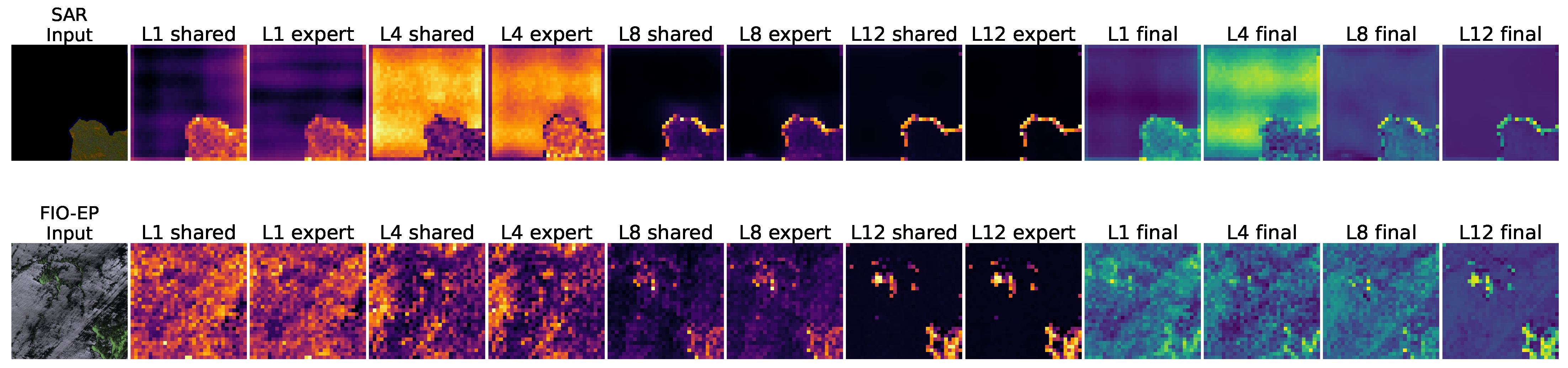
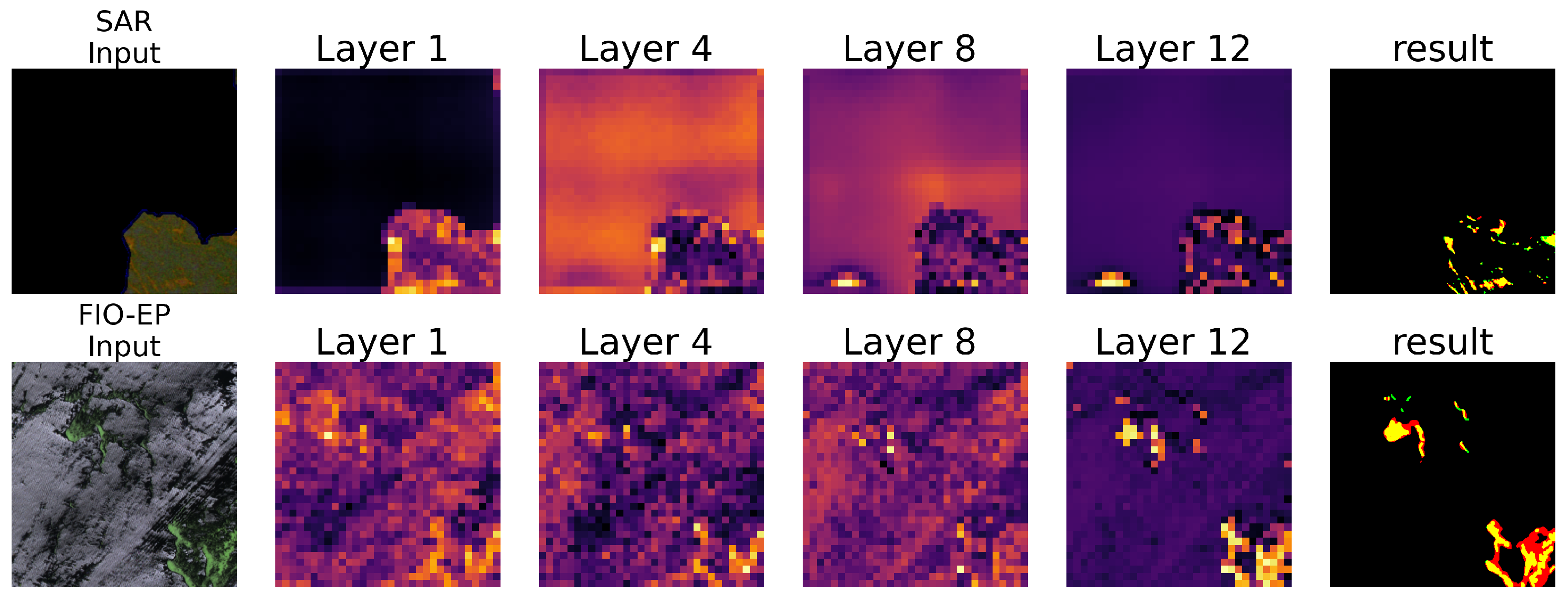
The visualization results of the shared feature, modality-specific feature, and fused aggregated feature are illustrated in Figure 8, which intuitively demonstrates the representation difference and complementary effect between the two branches. For each selected layer, the feature tensor is aggregated over the channel dimension via the L2 norm and normalized to [0, 1] by per-panel min–max scaling for display. The shared, expert, and final features have different channel widths (512, 256, and 768) and are normalized independently, so color only reflects the relative activation strength within each panel rather than cross-panel absolute values. The layer-by-layer visualization results reveal a clear hierarchical learning pattern of the proposed MoE encoder. In shallow layers, the shared branch dominantly extracts modality-agnostic low-level features such as edges and textures, while the expert branch provides negligible supplementary information. In middle and deep layers, the shared branch focuses on global Ulva prolifera localization and background suppression, whereas the modality-specific expert branches capture unique modal characteristics, including optical spectral textures and SAR polarization scattering features. In the deepest layer, the shared activations of both SAR and optical inputs are consistently concentrated on Ulva prolifera regions, demonstrating that the shared experts effectively learn general semantic priors; i.e., spatially abnormal feature areas highly correspond to Ulva prolifera distribution. Benefiting from this hierarchical two-branch modeling paradigm, the proposed method achieves superior segmentation performance in Ulva prolifera detection tasks. Multimodal comparison further indicates that the two modalities exhibit distinct expert activation characteristics. Due to severe speckle noise and complex scattering variations in SAR images, the expert branch undertakes more feature compensation work, yielding sparser and sharper activation responses. In contrast, optical images contain richer spectral and structural information, such that the shared branch already covers most effective feature representations. Accordingly, the optical expert branch mainly contributes to boundary refinement and detail optimization.

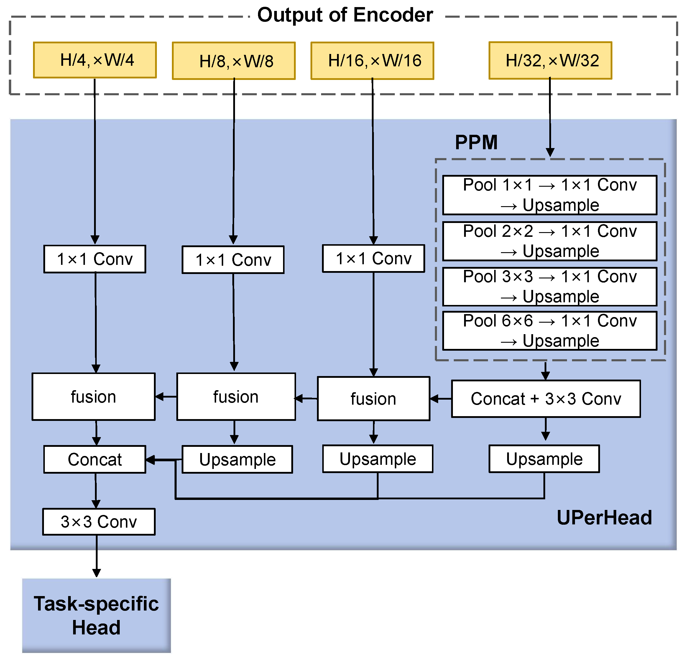
Figure 9 presents four groups of multi-scale feature maps output with progressively halved spatial resolutions by the ViT-MoE module. Feature normalization follows the same procedure as illustrated in Figure 8. The results show that optical images provide rich and clean original information, enabling the model to achieve faster feature convergence and more stable segmentation performance. In contrast, SAR images are severely affected by inherent speckle noise. The model requires deeper network layers to filter noise interference, resulting in slower feature convergence and occasional false segmentation. Nevertheless, the core Ulva prolifera regions can still be stably identified from SAR data. Under joint multimodal training, the deep features of both modalities consistently converge to green tide areas. This demonstrates that the model effectively learns modality-invariant Ulva prolifera representations, allowing the network to accurately locate target regions from both optical and SAR remote sensing data.

4. Discussion

The above experimental results demonstrate that the proposed DMDNet model achieves competitive performance on optical Ulva prolifera segmentation tasks and verify the effectiveness of the proposed model for multimodal remote sensing detection. The DMDNet model outperforms several mainstream unimodal segmentation models, including SegNet, U-Net, DeepLabV3+, ResUnet-a, and SegNeXt, in terms of three core segmentation evaluation metrics. In particular, our method achieves a superior mRecall of 0.9690, demonstrating a dominant advantage in foreground target detection.

The quantitative results across FIO-EP and CODC-optical demonstrate that our model obtains larger performance margins under more challenging conditions. Such gains mainly stem from superior foreground segmentation of Ulva prolifera rather than background fitting. Since overall accuracy aAcc becomes saturated under severe class imbalance, it cannot reliably reflect segmentation quality for green tide scenes.

Our model adopts a recall-prioritized inference regime, which fits the practical requirement of green tide monitoring where false negatives from missed algal patches incur higher operational risks than moderate false alarms. On CODC-optical, our approach even improves both precision and recall simultaneously, showing that multimodal training helps learn more discriminative Ulva features without sacrificing precision. In contrast, representative baselines show obvious dataset-dependent behaviors: multi-scale context models perform well on FIO-EP yet turn overly conservative on CODC-optical, while recent attention-driven networks suffer poor cross-dataset generalization.

Unlike the learning strategy of conventional single-modal models, the designed ViT-B/MoE structure incorporates both shared and modality-specific branches to alleviate feature entanglement between heterogeneous optical and SAR data, thereby fully exploiting the complementary advantages of dual-modal inputs. This enables the model to effectively capture fragmented, occluded, and low-contrast Ulva prolifera targets, minimize missed detections, and prioritize the integrity and comprehensiveness of green tide segmentation results. From the experimental results, such structural advantages fundamentally contribute to the comprehensive performance improvement on both the optical subset of FIO-EP and the CODC dataset compared with single-modal baselines.

Furthermore, the effectiveness of the designed multimodal comprehensive loss function has been evaluated by ablation experimental results. This loss function improves model performance mainly in two aspects. First, the spatial attention loss targets difficult segmentation regions by strengthening edge features and small-object responses, maintaining stable segmentation accuracy for extremely sparse algal samples. Second, the differentiated multimodal weight scheduling balances the joint training of optical and SAR branches, unifying gradient updates and avoiding performance bias caused by single-task dominance. Based on both qualitative and quantitative evaluations, the coordinated optimization of multiple loss terms enhances the segmentation accuracy for Ulva prolifera detection.

From the perspective of quantitative evaluation, the DMDNet model achieves a slightly lower precision than some unimodal methods due to the adopted fault-tolerant detection strategy, which introduces limited background false positives. Nevertheless, this precision–recall trade-off is highly reasonable for practical green tide monitoring tasks. In operational marine disaster monitoring, missed foreground targets will directly cause underestimation of green tide coverage, misjudgment of disaster severity, and failure of ecological early warning, leading to irreversible adverse impacts on marine ecological assessment and disaster prevention decision-making. In contrast, sporadic false-positive pixels can be effectively eliminated through simple post-processing strategies, such as multi-temporal consistency verification, morphological filtering, and marine region mask constraints. Therefore, the high-recall and fault-tolerant characteristics of the proposed model make it more suitable for practical green tide monitoring in complex and dynamic marine scenarios.

Despite the promising results achieved in this study, several technical challenges remain for constructing a high-precision multimodal intelligent monitoring system for marine environments. First, the model exhibits a noticeable performance bottleneck in SAR image segmentation. Future work will introduce polarimetric features to replace the conventional three-channel SAR input, so as to enrich the feature representation capability of SAR data. Second, this study only performs static feature modeling based on single-temporal optical and SAR data, without incorporating marine environmental factors such as sea surface temperature, wind speed, tides, and ocean currents. Further integration of multi-source environmental auxiliary data and time-series remote sensing information will help improve the model’s generalization ability under extreme marine conditions and sudden meteorological disturbances. It is worth noting that the 1×1 convolution employed in DMDNet only unifies the channel dimensions of optical and SAR features to facilitate subsequent joint processing. Although the shared ViT-MoE backbone can implicitly learn partial shared semantic information via joint gradient updates, there still exists a certain distribution gap between optical and SAR features. Accordingly, explicit domain-alignment optimization and quantitative validation of multimodal feature discrepancy will constitute important directions for our future research.

5. Conclusions

We develop a DMDNet model for accurate Ulva prolifera detection, which is capable of processing both optical and SAR data simultaneously. Equipped with an MoE mechanism and an optimized loss function, the DMDNet model effectively improved the multimodal feature modeling capacity and the fine-grained segmentation performance. Extensive experimental results demonstrate that the proposed model achieves stable and remarkable performance gains on the FIO-EP and CODC-optical datasets. Ablation experiments verify the effectiveness and complementarity of core modules, including the MoE mechanism and the customized loss function. Nevertheless, the detection accuracy of the DMDNet model on SAR datasets is inferior to that on optical datasets. Future research will focus on optimizations tailored to SAR application scenarios to further strengthen the multimodal generalization ability of the model, thereby providing more reliable technical support for Ulva prolifera detection.