Dual-Stream Spatial–Spectral Network with Nested Attention for Hyperspectral Image Classification

Highlights

What are the main findings?

• The DSSN obtains overall accuracies of 98.11%%, 99.88% and 99.82% on Indian Pines, Pavia University and Salinas, respectively, exceeding the tested CNN, Transformer and hybrid baselines.
• The ablation results demonstrate that all three components of the DSSN, the 3D-CNN stream, the nested Transformer branch, and the adaptive fusion module, contribute to improving the final classification performance.

What are the implications of the main findings?

• Separating local spectral–spatial extraction from contextual modelling helps reduce spectral confusion and fragmented predictions in benchmark HSI scenes.
• Channel-wise adaptive fusion offers a practical way to combine CNN-derived local details with Transformer-derived spatial context.

Abstract

Hyperspectral image classification (HSI) requires a model to distinguish subtle spectral differences while preserving the spatial structure of land-cover regions. CNN-based methods are effective for local spectral–spatial extraction, but their limited receptive fields can weaken broader context modelling. Transformer-based methods improve long-range dependency modelling, yet fixed patch partitioning may reduce their sensitivity to fine local structures. To address these limitations, this study proposes the Dual-Stream Spatial–Spectral Network with Nested Attention (DSSN), which separates local spectral–spatial feature extraction from multi-scale spatial-context modelling before adaptive fusion. The DSSN combines a cascaded 3D-CNN spectral stream, a nested Transformer spatial stream with pixel-level and patch-level interactions, and a channel-attention-based adaptive fusion module. Experiments on Indian Pines, Pavia University and Salinas show DSSN achieves overall accuracies of 98.11%%, 99.88% and 99.82%, respectively, outperforming other baselines. The ablation experiments confirm that each major component contributes to the final performance. Although the model requires more parameters and longer inference time than several compared baselines, its inference time remains at the millisecond level. These results suggest that decoupled spatial–spectral representation and adaptive multi-scale fusion can improve hyperspectral image classification under the evaluated benchmark settings.

1. Introduction

Hyperspectral imaging (HSI) records dense spectral responses for each spatial location, allowing materials with similar visual appearances to be distinguished more effectively than in RGB or multispectral imagery [1,2]. Compared with multispectral or RGB imaging, HSI provides many narrow spectral bands that can reveal subtle material differences. This capability has enabled important applications in precision agriculture [3,4,5], geological exploration [6], environmental monitoring [7], and urban planning [8]. Early HSI classification methods mainly relied on handcrafted features and shallow classifiers; these approaches are often insufficient for complex scenes because they have limited ability to learn nonlinear spectral–spatial representations [9,10]. Deep learning methods improved this situation by learning features directly from data; 1D-CNN models strengthened spectral modelling but treated pixels largely independently [11]; 2D-CNN models improved spatial texture extraction after dimensionality reduction, although part of the original spectral information could be lost [12]; 3D-CNN models further exploited the cube structure of HSI data by jointly processing adjacent spectral bands and neighboring pixels [13,14]. Later, contextual, recurrent and hybrid CNN models showed that spectral information and spatial context should be learned together rather than handled in isolation [15,16,17]. Since Transformers were introduced into computer vision, self-attention has been used to model long-range dependencies in HSI classification [18]. SpectralFormer was among the first Transformer backbones designed specifically for HSI, using grouped spectral embedding to model non-local spectral interactions [19]. However, it emphasizes global spectral correlations and pays less attention to fine-grained local spatial textures. To combine CNN-based local perception with Transformer-based global modelling, Sun et al. proposed SSFTT, a serial hybrid architecture that uses CNNs for feature extraction and Transformers for association modelling [20]. Although this design improves spatial–spectral complementarity, serial propagation can mix spatial and spectral information in ways that weaken subtle spectral cues. In addition, most ViT-based Transformers rely on fixed patch partitions, which limits their ability to represent multi-scale land-cover patterns [21].

These limitations motivate a model in which local spectral–spatial evidence and broader spatial context are learned as complementary representations. We therefore propose the Dual-Stream Spatial–Spectral Network with Nested Attention (DSSN). The spectral stream uses cascaded 3D-CNN layers to learn short-range spectral correlations and local micro-textures. The spatial stream uses a nested Transformer to connect pixel-level and patch-level contextual information. A block aggregation mechanism transfers local details into a wider spatial representation, and an adaptive fusion module (AFM) adjusts the contribution of the two streams through channel attention. In this way, DSSN does not simply stack convolution and self-attention, but assigns them different roles before adaptive fusion.

2. Materials and Methods

2.1. Proposed DSSN Architecture

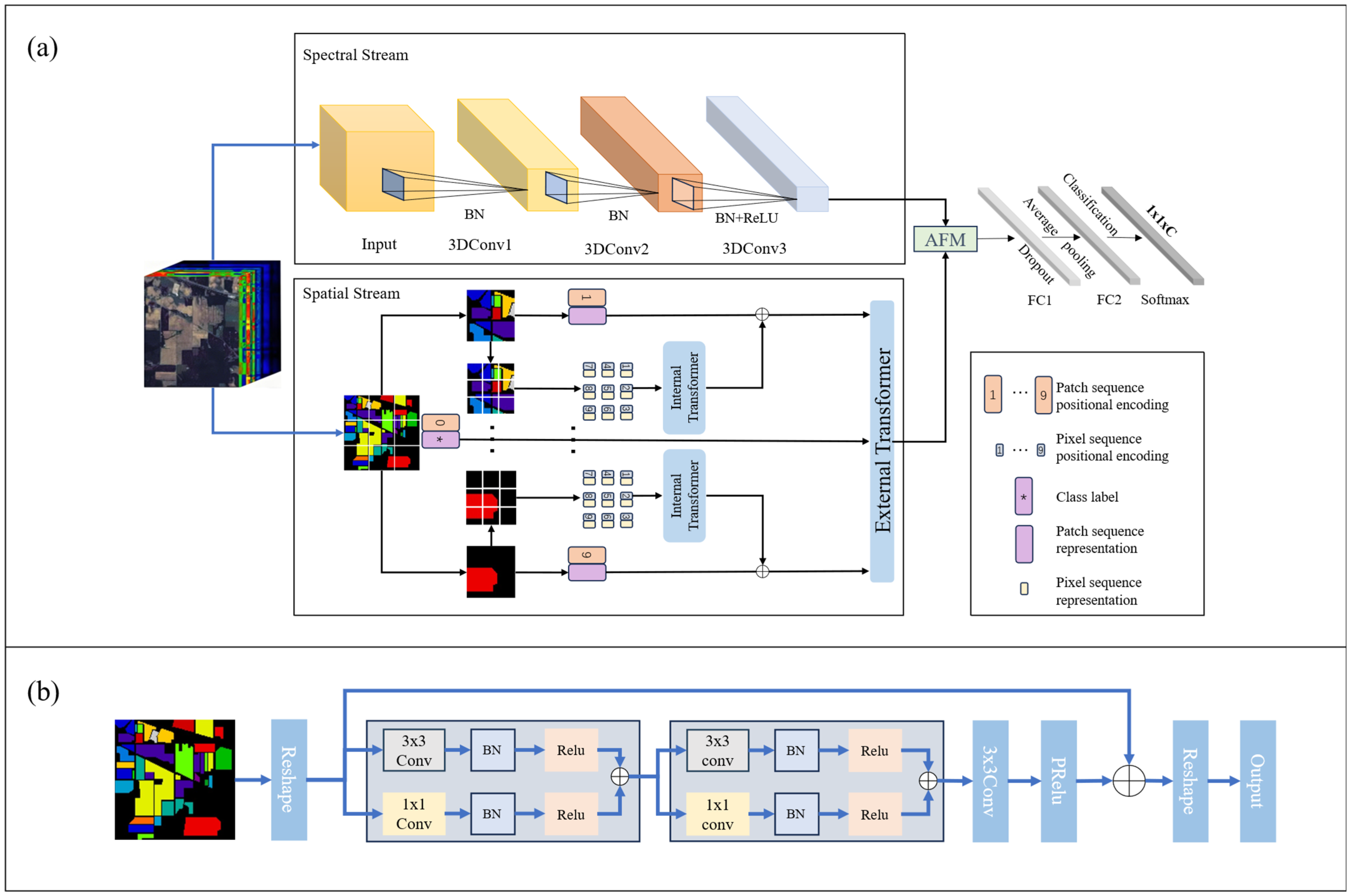
This section presents the structure of the DSSN and the role of each branch. The DSSN is organized around three core components, a 3D-CNN spectral stream for local spectral–spatial feature extraction, a nested Transformer spatial stream for multi-scale contextual modelling, and an AFM for dynamic feature integration. Given an input hyperspectral patch, the two streams learn complementary representations from different receptive-field ranges. The AFM then recalibrates and fuses these representations before the final classification layer. The spectral stream is designed to preserve short-range spectral correlations and local spectral–spatial structures. Hyperspectral data are naturally represented as volumetric cubes, and 3D convolutions are suitable for jointly processing neighboring spatial pixels and adjacent spectral bands. Therefore, this stream is built from cascaded 3D convolutional layers, as shown in Figure 1a.

Let the input feature map of the ${\left(l-1\right)}^{th}$ layer be $V^{l-1}$, with the dimensions of the feature maps being $H_{l-1}\times W_{l-1}\times D_{l-1}$; this layer contains $N_l$ 3D convolutional kernels, $K_{\dot{i}j}^l$, with $i$ indexing the current feature map and $j$ indexing the connected feature map from the previous layer. The activation of the $i^{th}$ feature map at spatial–spectral position $\left(x,y,z\right)$ in layer $l$, denoted as $v_{l,i}^{x,y,z}$, is computed as follows [22]:

$$v_{l,i}^{x,y,z}=\varphi \left({{\displaystyle \sum }}_{j=0}^{N_{l-1}-1}{{\displaystyle \sum }}_{p=0}^{P_l-1}{{\displaystyle \sum }}_{q=0}^{Q_l-1}{{\displaystyle \sum }}_{r=0}^{R_l-1}{w}_{l,i,j}^{p,q,r}\cdot v_{l-1,j}^{\left(x+p\right)\left(y+q\right)\left(z+r\right)}+b_{l,i}\right)$$

(1)

In this equation, $\varphi \left(\right)$ represents the nonlinear activation function. $N_{l-1}$ is the number of feature maps in the previous layer. $P_l{,Q}_l{,R}_l$ denote the height, width and spectral depth of the 3D convolution kernel, respectively. The kernel parameter is denoted by $w$, and b is the bias term. The indices $p,q,r$ specify positions inside the convolutional kernel, while $j$ indexes the connected feature map from the previous layer. Then, the spectral stream feature $F_{spec}$ is obtained with the shape $\left(B,C_1,H_C,W_c\right)$.

In DSSN, the spectral stream contains three 3D convolutional layers. To avoid excessive compression along the spectral dimension, the network uses valid padding spectrally and same padding spatially; this design progressively aggregates spectral information and produces a feature cube enriched with spectral features. Although the spectral stream captures local spectral–spatial patterns, its convolutional receptive field is limited. DSSN therefore introduces a nested Transformer spatial stream to model broader contextual dependencies. The module contains an inner pixel-level loop for fine local interactions and an outer patch-level loop for broader spatial relationships, allowing local details and global context to be represented within the same nested attention structure.

Assume the input to the DSSN is the preprocessed hyperspectral data cube $XϵR^{B\times D\times H\times W}$, where B, D, H, and W represent the batch size, the number of spectral bands, the input height, and the input width, respectively. When necessary, the input is padded along the bottom and right boundaries so that the padded height, $H^{\prime }$, and width, W′, are divisible by P. The outer-patch grid is defined as $G_h=H^{\prime }/\mathrm{P}$ and $G_w=W^{\prime }/\mathrm{P}$, and the number of outer patch tokens is $N_{\mathit{pat}}$. Each outer patch contains $N_{\mathit{pix}}={\left(P/\mathrm{p}\right)}^2$ pixel-level tokens. The input $X$ is mapped into two separate embedding spaces using the following formulas:

$$U_{pix}={\mathrm{Unfold}}_{k=p,s=p}\left(X_{\mathrm{outer}}\right)\in R^{B\times N_{pat}\times N_{\mathrm{pix}}\times D{p}^2}$$

(2)

$$Z_{pix}^0=U_{\mathrm{pix}}{W}_{\mathrm{pix}}+b_{\mathrm{pix}}+E_{pos}^{pix}\in R^{B\times N_{pat}\times N_{\mathrm{pix}}\times C_{\mathrm{pix}}}$$

(3)

$$U_{pat}=\mathrm{Flatten}\left(X_{\mathrm{outer}}\right)\in R^{B\times N_{pat}\times D{P}^2}$$

(4)

$$Z_{pat}^0=U_{pat}{W}_{pat}+b_{pat}+E_{pos}^{pat}\in R^{B\times N_{pat}\times C_{pat}}$$

(5)

The pixel-level branch applies a non-overlapping unfold operation within each outer patch. The resulting token sequence, $U_{\mathrm{pix}}$, has $N_{\mathit{pix}}$ tokens per outer patch, and each token contains the spectral values from a $p\times p$ spatial subregion. Therefore, the unprojected token dimension is $D{p}^2$. A learnable linear projection maps each token to the pixel-level embedding dimension, $C_{\mathit{pix}}$, producing $Z_{\mathit{pix}}^0$. In parallel, the patch-level branch flattens each outer patch into a single patch token. Each outer patch contains $D{p}^2$ values before projection, and the resulting patch-level sequence contains $N_{\mathit{pat}}$ tokens. The projected patch-level representation is denoted by $Z_{\mathit{pat}}^0$. This step establishes two parallel yet interconnected sequences: $Z_{pix}$ for capturing local details and $Z_{pat}$ for carrying global information.

In the $l^{th}$ nested attention block, Multi-Head Self-Attention (MSA) [22,23] is applied to model the local correlations between the pixels. The formula is as follows:

$${\widehat{Z}}_{pix}^l=Z_{pix}^{l-1}+\mathrm{MSA}\left(LN\left(Z_{pix}^{l-1}\right)\right)$$

(6)

where $Z_{pix}^{l-1}$ denotes the pixel-level feature entering the $l^{th}$ layer, and ${\widehat{Z}}_{pix}^l$ denotes the attention-updated intermediate representation. Subsequently, the DRNet is used in the feedforward block instead of a conventional Multi-Layer Perceptron (MLP) [24] to improve nonlinear feature extraction, as shown in Figure 1b, yielding the refined pixel features, $Z_{pix}^l$, output by the inner loop. The formula is as follows:

$$Z_{pix}^l={\widehat{Z}}_{pix}^l+\mathrm{DRNet}\left(LN\left({\widehat{Z}}_{pix}^l\right)\right)$$

(7)

As illustrated in Figure 1b, DRNet reshapes the input feature and then feeds it into two consecutive dual-branch blocks. Each block consists of two parallel branches, both comprising a convolutional layer, a batch normalization layer, and an ReLU activation function. The upper branch employs a $3\times 3$ convolution to capture local spatial information, whereas the lower branch uses a $1\times 1$ convolution to perform channel-wise feature transformation. The outputs of the two branches are fused through element-wise addition. After the two dual-branch blocks, the resulting feature is further refined by a $3\times 3$ convolution followed by a PReLU activation. A long residual connection adds the original reshaped feature to the refined feature, facilitating information preservation and stable feature learning. Finally, the fused feature is reshaped to produce the output. The primary purpose of DRNet is to refine the input features by combining local spatial feature extraction, channel-wise feature transformation, and residual learning. This design enhances feature representation while preserving the original information and improving the stability of network optimization.

To pass inner-loop details into the outer layer, the network aggregates pixel-level information along the spatial dimension to obtain an aggregated vector, $v_{agg}^l$. This operation is defined as follows:

$$v_{agg}^l=\mathcal{W}\left({\displaystyle \frac{1}{N}}{\displaystyle \sum _{i=1}^N{Z}_{pix}^l\left(i\right)}\right)$$

(8)

Here, $Z_{pix}^l\left(i\right)$ represents the pixel feature and $\mathcal{W}\left(\right)$ is a learnable linear projection matrix used to align the feature dimensions from $C_{pix}$ to $C_{pat}$.

The aggregated local representation, $Z_{pat}^{l-1}$, is then added to the patch-level feature to obtain an enhanced patch feature, $U_{pat}^l$, which integrates local details and serves as the input for the outer loop. The formula is as follows:

$$U_{pat}^l=Z_{pat}^{l-1}+v_{agg}^l$$

(9)

After obtaining the feature $U_{pat}^l$, a standard Transformer structure is utilized in the outer loop to model global contextual relationships, yielding the final patch feature, $Z_{pat}^l$, output by the $l^{th}$ nested block. This operation is defined as follows:

$${\widehat{Z}}_{pat}^l=U_{pat}^l+\mathrm{MSA}\left(LN\left(U_{pat}^l\right)\right)$$

(10)

$$Z_{pat}^l={\widehat{Z}}_{pat}^l+\mathrm{MLP}\left(LN\left(Z_{pat}^l\right)\right)$$

(11)

where the intermediate ${\widehat{Z}}_{pat}^l$ denotes the features after the attention mechanism. The number of nested attention layers and attention heads in the MSA modules used in Equations (6) and (10) are specified in

Table 1. Parameters of the Multi-Head Self-Attention modules.

Component	The Nested Attention	Patch-Level MSA	Pixel-Level MSA
Value	3	8	4

.

After processing through $L$ layers of nested blocks, the final patch sequence output is obtained. To align the final patch sequence with the spatial feature map generated by the 3D-CNN stream, a spatial reconstruction operation is performed. The resulting feature map, $F_{spat},$ is used as the output feature of the spatial stream, using the following formula:

$$F_{spat}=\mathcal{T}\left(LN\left(Z_{pat}^L\right)\right)\in R^{B\times C_2\times H_{\mathrm{s}}\times W_{\mathrm{s}}}$$

(12)

Here, $Z_{\mathit{pat}}^l$ denotes the final patch token sequence produced by the nested Transformer blocks. The operator $\mathcal{T}\left(\right)$ rearranges the sequence into the two-dimensional outer-patch grid of size $H_s\times W_s$, yielding $F_{spat}\in \left(B,C_2,H_{s,}{W}_s\right)$. After channel projection using $1\times 1$ convolutions, the spatial stream feature, $F_{spat}$, is bilinearly interpolated to match the spectral stream feature, $F_{spec}$. When the input dimensions are not divisible by the outer-patch size, boundary padding is used only to construct a complete token grid; a valid-region mask is generated simultaneously to distinguish the original input pixels from padded positions; the mask is propagated to the pixel-level aggregation and patch-level attention operations; therefore, the padded positions do not contribute to the aggregated representation or attention computation. After spatial interpolation, the valid-region mask is also applied before feature fusion, ensuring that the final prediction is determined only by the original input region.

After the spectral stream feature, $F_{spec}$, and the spatial stream feature, $F_{spat}$, are obtained, with shapes $\left(B,C_1,H_C,W_c\right)$ and $\left(B,C_2,H_C,W_c\right)$, respectively, the DSSN uses a channel-attention-based AFM to integrate them. The AFM is inspired by the squeeze-and-excitation mechanism, but is used here to recalibrate the relative contribution of the spectral and spatial streams during dual-stream fusion [25]. 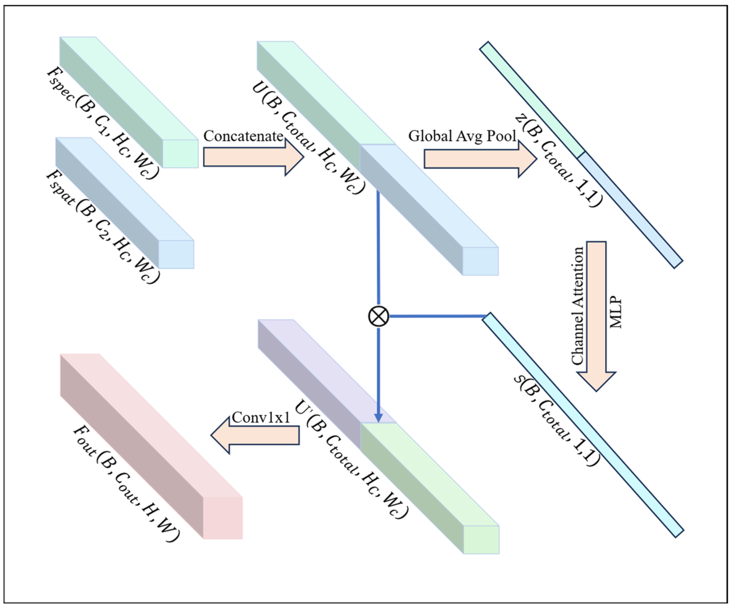Figure 2 shows the AFM workflow; the spectral and spatial feature maps are joined along the channel axis to obtain a mixed feature map, $U$, with the shape $\left(B,C_{total},H_C,W_c\right)$. This operation is defined as follows:

$$U=Concat\left(\right[F_{spec},F_{spat}\left]\right)$$

(13)

$$C_{total}=C_1+C_2$$

(14)

where $\mathrm{Concat}\left(\right)$ denotes the channel-wise joining of the two branch outputs.

To determine the importance of each channel, the representation is simplified. Instead of computing the value of every pixel, this part only requires the overall response intensity of the entire channel. Therefore, this network averages across the $H_C\times W_c$ spatial dimensions to obtain the global channel feature $z$, with a shape of $\left(B,C_{total},1,1\right)$; this vector represents the global distribution of the current sample across all feature channels, and the formula is as follows:

$$z=GlobalAvgPool\left(U\right)$$

(15)

Next, a small MLP is used to learn the dependencies between channels; the MLP reduces the number of channels to form a bottleneck representation and then restores the channel dimension. After restoring the channel count to $C_{total}$, the output values are mapped between 0 and 1 to obtain the attention weight vector, $s$, with a shape of $\left(B,C_{total},1,1\right)$, using the following formula:

$$s=\sigma \left(W_2\left(\delta \left(W_{1}z\right)\right)\right)$$

(16)

where $\sigma \left(\right)$ represents the Sigmoid activation function, $\delta \left(\right)$ represents the ReLU activation function, $W_1$ is the weight matrix of the first dimensionality reduction layer, and $W_2$ is the weight matrix of the second dimensionality reduction layer.

The generated weights are multiplied channel-by-channel with the original concatenated features to yield a new mixed feature map, $U^{\prime }$; important feature channels are enhanced, while unimportant or noisy channels are suppressed, using the following formula:

$$U^{\prime }=U\otimes s$$

(17)

Finally, these filtered features are blended using a $1\times 1$ convolution via linear combination, allowing the two streams to interact across channels; this operation compresses the fused channels, resulting in a more compact spatial output feature, $F_{out}$, using the following formula:

$$F_{out}=Con{v}_{1\times 1}\left(U^{\prime }\right)$$

(18)

the final feature, $F_{out}$, is mapped to the category space through fully connected layers, followed by a softmax function that outputs the class–probability distribution. The detailed implementation of the forward propagation of DSSN is presented in Algorithm 1.

Algorithm 1 Forward propagation of DSSN.
Input: Hyperspectral patch X ∈ RB×D×H×W Output: Predicted class yhat
1: S ← X	//B × D × H × W
2: S ← Conv3D(S)	//3D convolution
3: S ← BN(S); S ← ReLU(S)	//Spectral stream
4: S ← Conv3D(S)	//3D convolution
5: S ← BN(S); S ← ReLU(S)
6: S ← Conv3D(S)	//3D convolution
7: S ← BN(S); S ← ReLU(S)	//Spectral feature
8: Xp ← DivideIntoPatches(X, P)	//Patch size P × P
9: Q ← PixelEmbedding(Xp, p)	//Pixel window p × p
10: K ← PatchEmbedding(Xp)	//Patch representation
11: for l = 1, …, L do	//L nested blocks
12:     Q ← PixelTransformer(Q)	//Inner Transformer
13:     Q ← DRNet(Q)	//Local feature refinement
14:     K ← K + Aggregate(Q)	//Local-to-patch aggregation
15:     K ← PatchTransformer(K)	//Outer Transformer
16: end for
17: R ← SpatialReconstruction(K)	//Spatial feature map
18: R ← Resize (R, size(S))	//Match S and R
19: F ← Concatenate (S, R)	//Dual-stream feature
20: F ← AFM(F)	//Adaptive feature fusion
21: F ← AveragePooling(F)	//Global average pooling
22: F ← Dropout (F, r)	//Dropout rate r
23: F ← FC1(F)	//Fully connected layer
24: F ← FC2(F)	//Fully connected layer
25: y ← Softmax(F)	//K class probabilities
26: yhat ← Argmax(y)	//Predicted class
27: return yhat

2.2. Experimental Datasets

Indian Pines [26], Pavia University [27], and Salinas Valley [28] were used to test the model under different agricultural and urban scene conditions. To prevent spatial information leakage caused by overlapping neighborhoods, the labeled pixels were divided into spatially disjoint regions before neighborhood extraction. Of the labeled samples, 10% were used for training, and the remaining labeled samples were used for testing. A buffer zone corresponding to the neighborhood radius was retained between the training and testing regions.

• Indian Pines [26] was collected by the AVIRIS sensor (NASA Jet Propulsion Laboratory, Pasadena, United States) over an agricultural area in Indiana, USA, in June 1992. The scene contains 145 × 145 pixels and 220 spectral bands from 400 to 2500 nm. After removing 20 water absorption bands, 200 bands are retained. The reference map contains 16 land-cover categories, listed in

  Table 2. Classes and sample counts in the Indian Pines dataset.

  #	Class	Samples
  1	Alfalfa	46
  2	Corn-notill	1428
  3	Corn-mintill	830
  4	Corn	237
  5	Grass-pasture	483
  6	Grass-trees	730
  7	Grass-pasture-mowed	28
  8	Hay-windrowed	478
  9	Oats	20
  10	Soybean-notill	972
  11	Soybean-mintill	2455
  12	Soybean-clean	593
  13	Wheat	205
  14	Woods	1265
  15	Buildings-Grass-Trees-Drives	386
  16	Stone-Steel-Towers	93

  . Figure 3 shows the false-color image, grayscale representation and ground-truth map of the scene.
• The Pavia University dataset [27] was acquired by the ROSIS sensor (German Aerospace Center, Cologne, Germany) over Pavia, Northern Italy. It covers the 430–860 nm spectral range with a spatial resolution of 1.3 m. The image size is 610 × 340 pixels, and 103 spectral bands are used for training. The scene contains nine land-cover categories, as summarized in

  Table 3. Classes and sample counts in the Pavia University dataset.

  #	Class	Samples
  1	Asphalt	6631
  2	Meadows	18,649
  3	Gravel	2099
  4	Trees	3064
  5	Painted metal sheets	1345
  6	Bare Soil	5029
  7	Bitumen	1330
  8	Self-Blocking Bricks	3682
  9	Shadows	947

  . To complement the class statistics in Table 2, Figure 4 illustrates the Pavia University scene through its false-color image, grayscale representation, and ground-truth map.
• Salinas Valley [28] was captured by the AVIRIS sensor (NASA Jet Propulsion Laboratory, Pasadena, United States) over Salinas Valley, California. The scene has 512 × 217 pixels and a spatial resolution of 3.7 m. Of the original 224 bands, 204 remain after removing 20 water absorption bands. Sixteen land-cover classes are used, as shown in

  Table 4. Classes and sample counts in the Salinas Valley dataset.

  #	Class	Samples
  1	Brocoli_green_weeds_1	2009
  2	Brocoli_green_weeds_2	3726
  3	Fallow	1976
  4	Fallow_rough_plow	1394
  5	Fallow_smooth	2678
  6	Stubble	3959
  7	Celery	3579
  8	Grapes_untrained	11,271
  9	Soil_vinyard_develop	6203
  10	Corn_senesced_green_weeds	3278
  11	Lettuce_romaine_4wk	1068
  12	Lettuce_romaine_5wk	1927
  13	Lettuce_romaine_6wk	916
  14	Lettuce_romaine_7wk	1070
  15	Vinyard_untrained	7268
  16	Vinyard_vertical_trellis	1807

  . Figure 5 gives the false-color image, grayscale representation and ground-truth map.

2.3. Experimental Setup

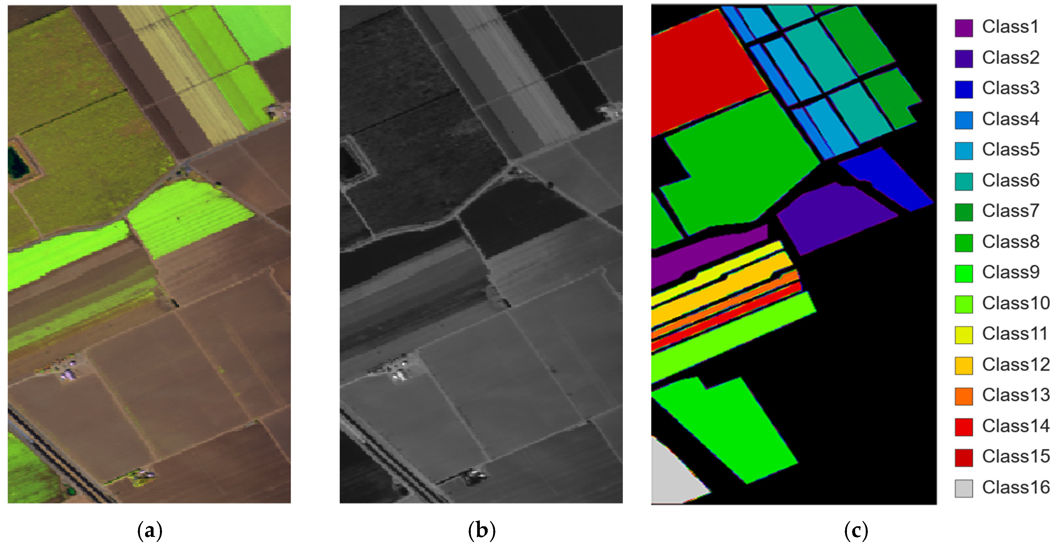
All experiments were implemented in PyTorch 2024.3.4 and conducted on a workstation equipped with an Intel Core i5-12400F CPU (Intel Corporation, Santa Clara, CA, USA), 16 GB RAM, and an NVIDIA GeForce GTX 1660 Ti GPU (NVIDIA Corporation, Santa Clara, CA, USA); the implementation used CUDA acceleration when available. To reduce the influence of random initialization and data partitioning, the random seeds of Python 3.9, NumPy 1.23.5, and PyTorch 2024.3.4 were fixed during training, and the cuDNN 8.9 backend was set to deterministic mode. For each hyperspectral dataset, the raw hyperspectral cube and its corresponding ground-truth map were loaded from mat files, only labeled pixels were used for training and testing, while background pixels with label value 0 were excluded from metric calculation. In the current implementation, each hyperspectral scene is first divided into a training region and a test region, after which normalization and patch extraction are performed. Specifically, the original hyperspectral scene is represented as $H\times W\times B$; after the data split, the training region is reshaped into $\left(H_{train}{W}_{train}\right)\times B$, and the minimum and maximum values are computed independently for each spectral band. The complete hyperspectral scene is then min–max-normalized using the statistics obtained exclusively from the training region, and the normalized data are reshaped back into the $H\times W\times B$ format. Then, fixed-size spatial–spectral patches are extracted from the normalized scene around the labeled center pixels in the original ground-truth map; these patches are assigned to the training or test set according to the partition to which their center pixels belong. The spatial patch size was set to 12 × 12, and the number of spectral channels depended on the dataset: 200 bands for Indian Pines, 103 bands for Pavia University, and 204 bands for Salinas. To ensure that pixels located at the image boundaries receive a fixed-size spatial neighborhood, we applied reflection padding to the two spatial dimensions of the normalized hyperspectral image before patch extraction. No padding was applied along the spectral dimension, and reflection padding mirrors the true pixels adjacent to the image boundaries to complete the missing neighborhood and does not introduce zero-valued or constant spectral vectors. For a labeled center pixel located at an image edge or corner, both its spatial coordinate and ground-truth label were retained from the original image; only the portion of its spatial neighborhood extending beyond the original image boundaries was supplemented with reflected values. Consequently, boundary pixels could be inferred using the same input size and model as interior pixels. Importantly, reflected pixels were not treated as additional training or testing samples, center coordinates were selected from the original ground-truth map using the condition gt > 0, and the train–test split was performed exclusively among these original labeled center pixels. The input of DSSN was constructed as a $12\times 12$ spatial–spectral patch centered on each labeled pixel. Within each local input patch, the Transformer stream partitions the patch into non-overlapping $6\times 6$ outer patches. Each outer patch is further divided into non-overlapping $3\times 3$ pixel-level subregions. Therefore, a $12\times 12$ input patch produces a $2\times 2$ outer-patch grid containing four patch-level tokens, while each outer patch contains four pixel-level tokens; for input dimensions that are not divisible by the outer patch size, reflection padding is applied before tokenization.

Therefore, each input sample retained both the local neighborhood structure and the complete spectral signature of the center pixel. To avoid overlap between training and testing neighborhoods, the image was partitioned into spatial blocks before sample extraction. Different blocks were assigned exclusively to the training or testing partition, and a buffer zone of at least 6 pixels was introduced along the partition boundary, corresponding to the radius of the 12 × 12 neighborhood. Labeled center pixels falling within this buffer zone were excluded from both partitions. Thus, no raw image pixel was shared by any training patch and testing patch. The labeled samples of each dataset were split in a class-wise manner; for every land-cover class, 10 percent of the samples in the designated training region were randomly selected for training, with at least 10 training samples retained per class. The remaining labeled samples were used for testing; this class-wise sampling strategy prevents large classes from dominating the split and ensures that small classes with very few samples still contribute to the training process.

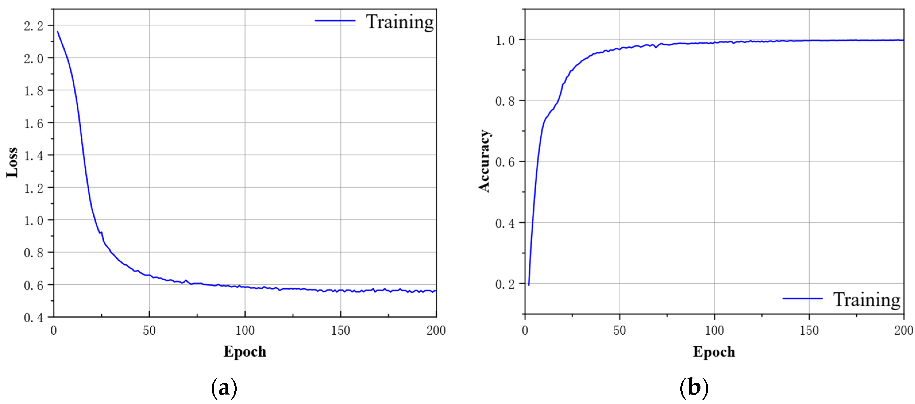
During training, simple spatial data augmentation was applied to the training patches, this included random horizontal flipping, random vertical flipping, and random rotations by multiples of 90 degrees; these operations preserve the spectral identity of the land-cover categories while increasing the spatial diversity of local neighborhoods. Such augmentation is particularly suitable for hyperspectral image classification because many land-cover classes are not sensitive to absolute orientation, but the model still needs to recognize them under different local spatial arrangements. The proposed DSSN was trained for 200 epochs with a batch size of 64; AdamW was used as the optimizer, with an initial learning rate of 1 × 10⁻³ and a weight decay of 1 × 10⁻⁴. To make the early training stage more stable, a warm-up strategy was adopted for the first 10% of the total epochs, after which a cosine annealing learning rate schedule was used, with the minimum learning rate set to 1 × 10⁻⁶. Cross-entropy loss with label smoothing was used for classification, and the label-smoothing factor was set to 0.1; the dropout rate in the final classifier was set to 0.5 to reduce overfitting; automatic mixed precision training was enabled to improve the computational efficiency of the GPU; gradient clipping with a maximum norm of 1.0 was applied to avoid the unstable updates caused by occasional large gradients; the model checkpoint was saved according to the monitored training loss and early stopping was used to prevent unnecessary training after convergence. The early stopping patience was set to 20 epochs in the main DSSN implementation. For repeated comparative experiments in the project records, each model dataset setting was run five times using different random seeds, and the mean and standard deviation were calculated from cycle runs; training data, including loss and training accuracy, were saved after training for convergence analysis; prediction maps were generated by applying the trained model to all labeled pixels in the scene, using the same patch extraction and reflection padding strategy as in training.

3. Experimental Results

3.1. Comparison with Baseline Methods

In the comparative experiments, the DSSN was evaluated against four representative HSI classification methods, 3D-CNN [14], HybridSN [17], SpectralFormer [19], SSFTT [20] and DSFormer [29]. These baselines cover convolutional, Transformer-based and hybrid spatial–spectral architectures. To ensure reproducibility, we used the publicly released code for each competing method to obtain the reported results.

• 3D-CNN [14] takes $5\times 5\times L$ spectral–spatial patches as input and is trained using the softmax loss and stochastic gradient descent with momentum. The momentum coefficient is set to 0.9, the weight decay coefficient to 5 × 10⁻⁴, and the batch size to 20.
• SpectralFormer [19] is optimized with Adam using minibatches of 64 samples. The learning rate starts at 5 × 10⁻⁴ and is reduced by a factor of 0.9 at every 10% interval of the total training epochs.
• SSFTT [20] reduces the hyperspectral data to 30 principal components using PCA and uses $13\times 13\times 30$ patches as input. It is trained with the Adam optimizer using an initial learning rate of 1 × 10⁻³, a batch size of 64, and 100 training epochs.
• HybridSN [17] was processed using 3D input patches with a spatial size of $25\times 25$ in all datasets, while the spectral dimensions were set to 30 for IP and 15 for UP and SA.
• DSFormer [29] was trained for 500 epochs using the AdamW optimizer, with an initial learning rate of 1 × 10⁻⁴ and a weight decay of 1 × 10⁻⁵. For all datasets, the input patch cubes were sized as $10\times 10$, the transformer patch size was set to 2, and the embedding dimension was fixed at 128.

Classification performance is evaluated using overall accuracy (OA), average accuracy (AA), and the Kappa coefficient (KA). Higher values indicate better classification performance. All methods were evaluated under the same dataset split and preprocessing protocol to ensure fair comparison.

On the Indian Pines dataset, as shown in

Table 5. Classification results of different methods on the Indian Pines.

#	3D-CNN [14]	SpectralFormer [19]	SSFTT [20]	HybridSN [17]	DSFormer [29]	DSSN
Class1	100.00	91.61 ± 7.07	96.10 ± 3.27	96.67 ± 3.04	93.17 ± 7.62	100.00
Class2	91.13 ± 2.53	74.16 ± 2.80	94.89 ± 2.98	94.70 ± 5.65	97.14 ± 1.29	98.32 ± 0.40
Class3	89.38 ± 7.93	60.87± 6.42	93.22 ± 3.89	93.86 ± 4.01	98.55 ± 0.78	97.48 ± 1.01
Class4	77.27 ± 19.14	84.81± 5.32	85.60 ± 1.76	80.93 ± 20.02	97.28 ± 2.58	96.64 ± 1.90
Class5	82.08 ± 14.83	85.68 ± 4.42	93.94 ± 5.48	90.18 ± 10.46	98.11 ± 1.80	96.28 ± 2.24
Class6	95.03 ± 5.36	88.91 ± 4.96	98.16 ± 1.29	98.82 ± 1.31	99.21 ± 0.22	99.70 ± 0.30
Class7	98.89 ± 2.48	89.23 ± 4.21	86.40 ± 1.43	100.00	90.40 ± 12.02	100.00
Class8	94.09 ± 7.14	96.68 ± 1.89	99.69 ± 0.43	98.79 ± 1.85	100.00	100.00
Class9	100.00	96.00 ± 8.94	82.22 ± 4.02	100.00	81.11 ± 15.15	100.00
Class10	90.73 ± 7.36	74.88 ± 3.95	91.16 ± 6.11	96.15 ± 2.84	97.19 ± 1.79	96.80 ± 1.58
Class11	93.57 ± 1.55	73.55 ± 4.92	94.69 ± 3.01	97.15 ± 1.22	97.23 ± 1.11	98.62 ± 0.64
Class12	75.72 ± 15.71	68.66 ± 9.25	84.62 ± 9.32	90.78 ± 6.40	95.17 ± 3.06	93.82 ± 4.65
Class13	94.67 ± 5.01	98.45 ± 0.74	97.54 ± 2.69	95.91 ± 3.62	99.24 ± 0.25	98.27 ± 1.49
Class14	97.84 ± 1.64	78.93 ± 6.02	97.94 ± 2.09	99.07 ± 0.79	99.68 ± 0.19	99.70 ± 0.21
Class15	80.16 ± 13.42	79.16 ± 3.72	88.77 ± 7.77	88.83 ± 5.82	98.73 ± 1.55	99.14 ± 0.75
Class16	94.69 ± 3.26	97.67 ± 1.64	90.24 ± 5.52	85.30 ± 9.27	98.57 ± 1.90	91.54 ± 4.59
OA (%)	90.88 ± 3.10	76.86 ± 1.61	94.07 ± 2.34	95.36 ± 0.03	97.86 ± 0.25	98.11 ± 0.37
AA (%)	90.95 ± 4.33	83.70 ± 1.58	92.20 ± 5.18	94.19 ± 0.04	96.30 ± 1.12	97.89 ± 0.46
KA (%)	89.59 ± 3.56	73.62 ± 0.02	93.24 ± 2.72	94.71 ± 0.03	97.56 ± 0.29	97.84 ± 0.42

, DSSN achieved an OA of 98.11%, an AA of 97.89%, and a Kappa coefficient of 97.84%, obtaining the highest values among all compared methods; compared with the strongest baseline, DSFormer, the DSSN improved OA, AA, and Kappa by 0.25, 1.59, and 0.28 percentage points, respectively. The relatively larger improvement in AA indicates that the DSSN provides more balanced recognition performance across different land-cover categories, rather than improving only the dominant classes. Although DSFormer achieved slightly higher accuracy for several individual classes, the DSSN produced the best overall performance and maintained relatively stable results across repeated experiments, as reflected by its small standard deviations for OA, AA, and Kappa. The visual comparison in Figure 6 further shows that the DSSN reduces isolated misclassified pixels and better preserves the spatial continuity of agricultural parcels, which is consistent with the improvements in the quantitative evaluation.

As shown in

Table 6. Classification results of different methods on the Pavia University dataset.

#	3D-CNN [14]	Spectral Former [19]	SSFTT [20]	HybridSN [17]	DSFormer [29]	DSSN
Class1	91.39 ± 6.19	93.28 ± 1.56	90.62 ± 5.01	97.44 ± 1.26	95.87 ± 1.13	99.83 ± 0.16
Class2	94.19 ± 4.19	95.85 ± 2.07	96.56 ± 2.77	99.28 ± 0.62	97.60 ± 1.19	99.98 ± 0.02
Class3	92.14 ± 4.80	85.73 ± 1.90	90.72 ± 3.63	97.10 ± 1.75	94.46 ± 2.70	99.97 ± 0.05
Class4	95.02 ± 1.86	88.02 ± 3.05	91.42 ± 8.10	99.26 ± 1.35	97.57 ± 1.10	99.25 ± 0.32
Class5	99.88 ± 0.28	99.27 ± 0.26	99.30 ± 0.77	100.00	99.97 ± 0.06	100.00
Class6	97.89 ± 1.77	88.95 ± 1.74	96.44 ± 3.37	98.68 ± 2.57	98.24 ± 0.75	100.00
Class7	99.72 ± 0.39	83.64 ± 2.44	98.85 ± 1.15	99.79 ± 0.35	99.82 ± 0.22	99.93 ± 0.11
Class8	90.46 ± 2.99	78.46 ± 4.03	90.33 ± 2.02	94.73 ± 4.43	95.01 ± 3.03	99.79 ± 0.13
Class9	97.90 ± 1.42	99.93 ± 0.10	98.54 ± 1.15	99.27 ± 0.48	99.21 ± 0.68	99.55 ± 0.37
OA (%)	94.25 ± 2.05	91.91 ± 0.99	94.63 ± 1.76	98.25 ± 0.74	97.21 ± 0.57	99.88 ± 0.04
AA (%)	95.40 ± 1.25	90.35 ± 0.58	94.75 ± 1.70	98.05 ± 0.91	97.53 ± 0.32	99.81 ± 0.06
KA (%)	92.46 ± 2.64	89.27 ± 1.28	92.92 ± 2.31	97.67 ± 0.99	96.31 ± 0.74	99.84 ± 0.05

, DSSN achieved an OA of 99.88%, an AA of 99.81%, and a Kappa coefficient of 99.84% on the Pavia University dataset. Relative to the strongest baseline, HybridSN, DSSN improved OA, AA, and Kappa by 1.63, 1.76, and 2.17 percentage points, respectively. Pavia University contains complex urban structures, including roads, buildings, bare soil, and elongated object boundaries. The strong gains in all three aggregate metrics suggest that the dual-stream architecture effectively combines local spectral–spatial feature extraction with broader contextual modelling. As illustrated in Figure 6, the DSSN generates more spatially coherent classification maps, reduces fragmented predictions around object boundaries, and better maintains the continuity of road- and building-related regions.

As shown in

Table 7. Classification results of different methods on the Salinas Valley dataset.

#	3D-CNN [14]	Spectral Former [19]	SSFTT [20]	HybridSN [17]	DSFormer [29]	DSSN
Class1	99.92 ± 0.18	99.87 ± 0.14	99.98 ± 0.02	100.00	100.00	100.00
Class2	99.81 ± 0.25	98.03 ± 1.83	99.92 ± 0.17	99.81 ± 0.42	100.00	100.00
Class3	99.56 ± 0.40	98.99 ± 0.26	100.00	99.98 ± 0.02	99.93 ± 0.10	99.67 ± 0.58
Class4	99.56 ± 0.51	99.47 ± 0.26	99.18 ± 0.71	99.88 ± 0.17	99.38 ± 0.49	99.41 ± 0.75
Class5	97.95 ± 1.93	98.43 ± 0.84	99.36 ± 0.72	98.05 ± 1.54	98.56 ± 1.30	99.96 ± 0.05
Class6	99.66 ± 0.71	99.86 ± 0.07	99.97 ± 0.04	100.00	100.00	99.97 ± 0.06
Class7	99.76 ± 0.34	99.59 ± 0.14	99.92 ± 0.15	99.91 ± 0.13	99.86 ± 0.16	100.00
Class8	86.93 ± 4.20	89.49 ± 1.59	88.08 ± 1.75	95.74 ± 1.25	86.18 ± 5.11	99.74 ± 0.13
Class9	99.88 ± 0.26	99.84 ± 0.11	100.00	99.99 ± 0.01	99.98 ± 0.02	100.00
Class10	98.22 ± 1.21	94.30 ± 1.21	97.64 ± 1.30	99.06 ± 0.67	97.31 ± 1.37	99.70 ± 0.36
Class11	99.57 ± 0.35	97.92 ± 0.96	99.94 ± 0.08	100.00	100.00	99.56 ± 0.81
Class12	100.00	98.47 ± 1.30	99.70 ± 0.31	99.97 ± 0.04	99.98 ± 0.02	100.00
Class13	99.97 ± 0.05	97.31 ± 2.17	99.75 ± 0.36	99.98 ± 0.05	100.00	99.42 ± 0.69
Class14	99.59 ± 0.31	95.29 ± 2.48	98.87 ± 1.26	99.86 ± 0.27	99.85 ± 0.13	99.85 ± 0.14
Class15	94.29 ± 2.09	58.12 ± 6.34	94.35 ± 2.35	94.79 ± 3.81	94.81 ± 2.35	99.61 ± 0.32
Class16	99.36 ± 0.38	98.31 ± 0.81	99.05 ± 0.81	99.39 ± 0.52	99.79 ± 0.16	99.90 ± 0.09
OA (%)	96.13 ± 0.11	91.23 ± 0.56	96.46 ± 0.49	98.19 ± 0.44	96.13 ± 0.97	99.82 ± 0.08
AA (%)	98.38 ± 0.48	95.21 ± 0.33	98.48 ± 0.27	99.15 ± 0.32	98.48 ± 0.33	99.80 ± 0.09
KA (%)	95.69 ± 0.12	90.21 ± 0.01	96.07 ± 0.55	97.97 ± 0.49	95.70 ± 1.07	99.80 ± 0.09

, the DSSN also achieved a strong performance on Salinas, with an OA of 99.82%, an AA of 99.80% and a KA of 99.80%. Salinas is a high-accuracy benchmark on which several methods already perform well, making further improvements difficult. Compared with the strongest baseline, HybridSN, the DSSN improved OA by 1.63 percentage points; the improvement is especially relevant for visually and spectrally similar agricultural categories, including lettuce- and vineyard-related classes. The visual comparison in Figure 6 shows that the DSSN reduces within-field noise and better separates neighboring agricultural categories. This improvement is particularly relevant for Salinas, where several crop classes have similar spectral responses and many baseline methods already achieve high overall accuracy.

Figure 7 shows the accuracy and loss curves over 200 training epochs on the Pavia University dataset; the training loss and accuracy curves are similar to those of the other two datasets. The DSSN converges rapidly during the early epochs and then enters a stable optimization stage. The loss curve flattens after approximately 100 epochs, while the accuracy approaches saturation, indicating that the proposed dual-stream architecture does not introduce obvious training instability.

The ROC analysis further supports the performance of the DSSN across the three datasets, as shown in Figure 8. The DSSN achieves an AUC of 0.9999 on Indian Pines, Pavia University and Salinas, indicating that its predictions provide near-perfect ranking of positive and negative samples under the evaluated test conditions. On Indian Pines, the DSSN yields a higher AUC than 3D-CNN, DSFormer, HybridSN, SpectralFormer and SSFTT, whose AUC values are 0.9971, 0.9997, 0.9897, 0.9835 and 0.9966, respectively. The advantage is particularly evident over SpectralFormer and HybridSN, whereas the difference from DSFormer is small. Similar results are observed on Pavia University and Salinas, where the DSSN exceeds the strongest competing methods by 0.0007 and 0.0002 AUC units, respectively. These results suggest that the combination of local spectral–spatial modelling, nested spatial-context extraction and adaptive feature fusion enables DSSN to maintain strong class separability across agricultural and urban hyperspectral scenes.

3.2. Computational Complexity Analysis

The computational cost of DSSN was evaluated using both model-level and component-level analysis.

Table 8. Computational complexity comparison of different models.

Dataset	Method	Parameters (M)	Inference Time (ms)	Training Time (min)
Indian Pines	3D-CNN	0.4793	2.8036	7.30
	SpectralFormer	0.3464	3.9156	9.18
	SSFTT	0.6752	2.4870	4.63
	HybridSN	0.8256	3.4550	8.45
	DSFormer	0.7902	3.6420	8.94
	DSSN	1.327	5.5657	10.67
Pavia University	3D-CNN	0.3315	3.0536	9.60
	SpectralFormer	0.1619	4.3896	34.07
	SSFTT	0.3532	2.5330	10.91
	HybridSN	0.6467	3.7445	19.29
	DSFormer	0.6779	3.7274	13.10
	DSSN	1.1057	6.4070	28.33
Salinas Valley	3D-CNN	0.4543	3.4325	11.49
	SpectralFormer	0.3563	4.6221	38.40
	SSFTT	0.4837	2.4872	13.44
	HybridSN	0.8329	3.7366	22.97
	DSFormer	0.7857	3.8156	18.67
	DSSN	1.340	6.0038	32.33

compares DSSN with the baseline methods, and Figure 8 decomposes the FLOPs of the proposed architecture.

Table 8 compares the computational complexity of the DSSN with five representative models, including 3D-CNN, SpectralFormer, SSFTT, HybridSN and DSFormer; the comparison is conducted on the Indian Pines, Pavia University and Salinas Valley datasets in terms of the number of parameters, average single-sample inference time and average training time. The DSSN contains 1.327 M, 1.1057 M and 1.340 M parameters on the three datasets, respectively; its average parameter size is approximately 1.26 M, which is higher than that of the other compared models. This increase is mainly caused by the simultaneous use of the 3D-CNN spectral stream, the nested Transformer spatial stream and the adaptive fusion module. The average inference times of the DSSN are 5.5657 ms, 6.4070 ms and 6.0038 ms on Indian Pines, Pavia University and Salinas Valley, respectively. The DSSN is slower than most competing methods, due to its dual-stream architecture and nested attention operations. In terms of training time, the DSSN requires 10.67 min, 28.33 min and 32.33 min on Indian Pines, Pavia University and Salinas Valley, respectively. The longer training time is mainly related to the larger model size and the additional Transformer-based spatial-context modelling; thanks to the early-stopping mechanism, although its training time is longer than the other models, it is comparable to that of SpectralFormer. Overall, the results show that DSSN achieves improved representation capability at the cost of increased parameters, inference time and training time.

Figure 9 further decomposes the FLOPs of DSSN at the component level: Figure 9a compares different component configurations on Indian Pines, Pavia University and Salinas, showing that the relative FLOPs pattern remains consistent across datasets despite their different spectral dimensions. Figure 9b summarizes the mean FLOPs across the three datasets, where the full DSSN model reaches 0.2640 G, which is only 0.0072 G higher than the CNN-only configuration and 0.0003 G higher than the simple-fusion configuration. Figure 9c further shows the incremental cost of each component: the CNN branch accounts for most of the FLOPs, the Transformer branch adds a small increment, and AFM contributes only 0.0003 G additional FLOPs. These results indicate that the additional computational burden of the DSSN mainly comes from maintaining the dual-stream representation, not from the adaptive fusion operation itself.

3.3. Ablation Experiments

Ablation Experiments were used to examine the role of each DSSN module on the three datasets; four components were examined, namely the 3D-CNN spectral stream, DRNet, the nested Transformer module and the AFM. It is worth noting that, when both DRNet and the nested Transformer are removed, the nested Transformer is replaced with a standard Transformer. When AFM is removed, a simple fusion strategy is used instead. The OA results for each configuration are summarized in

Table 9. Ablation results of the main DSSN components on the three datasets.

CNN	DRNet	Nested Trans	AFM	Indian Pines	Pavia University	Salinas Valley
× *	√ *	√	√	96.91	96.75	97.37
√	×	√	√	97.77	98.42	98.92
√	√	×	√	97.06	97.64	97.69
√	×	×	√	96.23	96.83	96.14
√	√	√	×	97.48	98.89	99.05
√	√	√	√	98.11	99.88	99.82

* √ indicates the corresponding module is included, whereas × indicates it is excluded

.

Table 9 reports the ablation results of the main components of the DSSN, including the 3D-CNN spectral stream, DRNet, the nested Transformer and the AFM. The configuration without the main components obtains OA of 96.91%, 96.75% and 97.37% on Indian Pines, Pavia University and Salinas Valley, respectively. After incorporating the complete DSSN architecture, the OA increases to 98.11%, 99.88% and 99.82%, corresponding to improvements of 1.20, 3.13 and 2.45 percentage points, respectively. The intermediate configurations also provide useful evidence for analyzing the contribution of each component. On the Indian Pines dataset, the OA values of these configurations range from 97.06% to 97.77%, on the Pavia University dataset, the range is from 96.23% to 98.92%, and on the Salinas Valley dataset, the range is from 96.14% to 99.05%. These results indicate that the performance improvement is not driven by a single module but rather stems from the synergistic effects of local spectral–spatial feature extraction, spatial-context modeling, and adaptive feature fusion.

3.4. Parameter Sensitivity Analysis

Table 10. Impact of the input spatial window size on DSSN.

Window Size	Indian Pines	Pavia University	Salinas Valley
6 × 6	97.94	99.81	99.75
9 × 9	97.96	99.85	99.78
12 × 12	98.11	99.88	99.82

evaluates the influence of the input spatial window size on DSSN. Three window sizes were compared on the Indian Pines, Pavia University and Salinas Valley datasets. The results show that increasing the spatial window size consistently improves the classification performance on all three datasets. When the window size increases from 6 × 6 to 12 × 12, the OA improves from 97.94% to 98.11% on Indian Pines, from 99.81% to 99.88% on Pavia University, and from 99.75% to 99.82% on Salinas Valley. Thus, the corresponding improvements are 0.17, 0.07 and 0.07 percentage points, respectively. This result indicates that a larger spatial window provides the DSSN with more surrounding contextual information, which benefits both the local spectral–spatial extraction of the 3D-CNN stream and the multi-scale spatial modelling of the nested Transformer stream. The additional context is particularly useful for distinguishing neighboring land-cover categories and maintaining spatial continuity near object boundaries.

Table 11. Impact of the channel compression ratio of the AFM on DSSN.

Ratio	Indian Pines	Pavia University	Salinas Valley
2	98.13	99.84	99.79
4	98.11	99.85	99.78
8	97.95	99.73	99.73

investigates the influence of the channel compression ratio in the AFM; three compression ratios were evaluated on the three datasets, and the results demonstrate that the compression ratio has a relatively limited influence on the final OA when moderate compression is applied. For Indian Pines, the model achieves the highest OA of 98.13% with a compression ratio of 2, for Pavia University, the highest OA is 99.85% with a ratio of 4, while the best result on Salinas Valley is 99.79% with a ratio of 2; the performance obtained with compression ratios of 2 and 4 is highly comparable. These results suggest that a moderate compression ratio provides a suitable balance between channel interaction and feature compactness.

4. Discussion

The DSSN addresses the challenge of simultaneously preserving locally discriminative spectral information and large-scale spatial context in hyperspectral image classification. It employs a dual-stream framework consisting of a 3D-CNN branch, a nested Transformer branch and an AFM. By exploiting local connectivity and weight sharing, the 3D-CNN branch jointly processes the spectral and spatial dimensions, preserving local spectral–spatial evidence from adjacent bands, neighboring pixels and fine-grained textures. In parallel, the nested Transformer branch performs pixel-level interaction, local information aggregation and patch-level context modelling. This design progressively propagates fine-grained local features into broader spatial representations and enables hierarchical contextual reasoning from local to global scales. The AFM generates channel-wise weights from the joint responses of each input sample and dynamically adjusts the contributions of local and contextual features before classification. Thus, the three modules form a complete information-processing pipeline based on local joint representation learning, hierarchical context modelling and sample-conditioned feature fusion. Consistent with this design, the DSSN achieves OAs of 98.11%, 99.88% and 99.82% on the Indian Pines, Pavia University and Salinas Valley datasets, respectively, demonstrating stable performance across different agricultural and urban hyperspectral scenes.

The DSSN differs from previous methods, not only by combining CNNs with Transformers, but also through its representational specialization and information-flow topology. Pure 3D-CNNs enlarge their receptive fields through repeated local convolutions, meaning that long-range spatial relationships are established only indirectly. Pure Transformer and SpectralFormer-like methods model non-local dependencies, but fixed-scale token representations may weaken local spectral continuity and fine-grained spatial textures. Serial CNN–Transformer methods, such as SSFTT, apply Transformer-based modelling to features that have already undergone convolutional projection, making it difficult for local and contextual information to be propagated independently. Conventional dual-stream classifiers generally divide the network into separate spectral and spatial branches and fuse their outputs through direct addition, feature concatenation or fixed-form weighting. In contrast, DSSN divides feature learning according to the effective range of information. The 3D-CNN branch learns local joint spectral–spatial features, whereas the nested Transformer branch captures hierarchical contexts from pixel-level interactions to patch-level representations. The two pathways are preserved during their respective feature-learning processes and interact only during the fusion stage, thereby reducing premature mixing at shallow layers. The ablation results in Table 9 support the contribution of this information-flow design. The minimum configuration obtains OAs of 96.91%, 96.75% and 97.37% on Indian Pines, Pavia University and Salinas Valley, whereas the complete DSSN achieves 98.11%, 99.88% and 99.82%, respectively. The corresponding improvements are 1.20, 3.13 and 2.45 percentage points, indicating that the 3D-CNN stream, DRNet, nested Transformer and AFM provide complementary benefits. The 3D-CNN stream preserves local spectral–spatial evidence, DRNet enhances nonlinear pixel-level feature transformation, the nested Transformer establishes local-to-global spatial relationships, and the AFM adaptively recalibrates the channel-wise contributions of the two streams. Therefore, the gain of the DSSN arises from the interaction among these modules rather than from the isolated effect of a single component. The parameter sensitivity experiments further support the selected design settings. As shown in Table 10, increasing the input spatial window from 6 × 6 to 12 × 12 improves the OA from 97.94% to 98.11% on Indian Pines, from 99.81% to 99.88% on Pavia University and from 99.75% to 99.82% on Salinas Valley. The 12 × 12 window is therefore selected because it provides a broader contextual range and achieves the best performance on all three datasets. Table 11 shows that compression ratios of 2 and 4 produce nearly identical classification accuracy, whereas a ratio of 8 causes a performance decrease on all datasets. Although a ratio of 2 achieves slightly higher accuracy on some datasets, it retains a larger intermediate channel dimension and introduces greater computational cost. Considering both accuracy and efficiency, a compression ratio of 4 is selected for the AFM. The improvement pattern differs across datasets. On Indian Pines and Pavia University, the DSSN provides modest but consistent gains over HybridSN, with OA improvements of 0.46 and 0.47 percentage points, respectively. On Salinas, the improvement is more pronounced, reaching 2.22 percentage points over HybridSN. This pattern suggests that nested contextual modelling and adaptive fusion are particularly useful when fine agricultural class discrimination is required, while still providing stable gains in fragmented agricultural and urban scenes. The ablation experiments support this interpretation. The 3D-CNN stream improves performance by preserving local spectral–spatial information, the nested Transformer contributes broader contextual modelling, and AFM further improves performance by recalibrating the contribution of the two streams. These findings suggest that the observed performance gain arises from the interaction between decoupled representation learning and adaptive fusion, rather than from any single module alone.

The computational results reveal the practical trade-offs associated with the proposed architecture: DSSN contains 1.327 M, 1.1057 M and 1.340 M parameters on the Indian Pines, Pavia University and Salinas Valley datasets, respectively; its single-sample inference times are 5.5657 ms, 6.4070 ms and 6.0038 ms, with corresponding training times are 10.67 min, 28.33 min and 32.33 min; the increased computational cost is mainly attributable to the dual-stream architecture and the nested attention operations. Therefore, future work will investigate strategies for reducing the computational cost of the DSSN. In addition, real-world hyperspectral images are often affected by Gaussian noise, impulse noise, stripe noise and mixed noise. The robustness of the network is therefore particularly important under noisy hyperspectral conditions. In future work, we will systematically investigate the effects of Gaussian, impulse, stripe and mixed noise on hyperspectral image classification [30,31], as well as seeking to develop effective methods for suppressing and removing hyperspectral noise.

5. Conclusions

This study proposed the Dual-Stream Spatial–Spectral Network with Nested Attention (DSSN) for hyperspectral image classification. By combining a cascaded 3D-CNN spectral stream, a nested Transformer spatial stream and an adaptive fusion module, the DSSN separates local spectral–spatial feature extraction from multi-scale contextual modelling and adaptively integrates the resulting representations. Experiments on Indian Pines, Pavia University and Salinas showed that the DSSN outperformed representative CNN-, Transformer- and hybrid-based baselines, achieving 98.11%%, 99.88% and 99.82% OA, respectively. Ablation experiments further confirmed that the 3D-CNN stream, nested Transformer and AFM each contributed to the final performance. These findings suggest that decoupled spatial–spectral learning with adaptive multi-scale fusion is effective for HSI classification, particularly in scenes requiring fine spectral discrimination and spatial boundary preservation. However, the increased computational cost and the potential impact of noise should be carefully considered when deploying the DSSN in real-world hyperspectral image classification scenarios.