Article

Land-Use Change and Land-Cover-Based Ecological Quality Patterns in a Coal Resource-Based City: A Case Study of Ordos, China

College of Geoscience and Surveying Engineering, China University of Mining and Technology-Beijing, Beijing 100083, China
*
Author to whom correspondence should be addressed.
Remote Sens. 2026, 18(18), 3131; https://doi.org/10.3390/rs18183131
Submission received: 18 August 2026 / Revised: 9 September 2026 / Accepted: 10 September 2026 / Published: 11 September 2026
(This article belongs to the Section Environmental Remote Sensing)

Highlights

What are the main findings?
  • A 25-year Landsat-based land-use dataset was produced for Ordos, China, with mining areas mapped as an independent land-use class.
  • Mining and built-up land expanded markedly, while the land-cover-based ecological quality index showed a decline-recovery-stabilization pattern from 2000 to 2025.
What are the implications of the main findings?
  • The task-oriented U-Net improves land-use mapping in complex mining areas, while treating mining areas as an independent class enables clearer identification of mining expansion and land-use conversions.
  • The framework combining land-use transition analysis, EQI, and LEI can support land-cover-based ecological monitoring in Ordos and comparable coal resource-based cities in arid and semi-arid regions.

Abstract

This study investigated the long-term relationship between land-use change and land-cover-based ecological quality patterns in Ordos City, a typical coal resource-based city in northern China. To explicitly capture land-use transitions driven by coal exploitation, mining areas were classified as an independent land-cover type. An improved U-Net semantic segmentation model integrating multispectral information and land surface temperature was subsequently employed to generate multi-temporal land-cover maps. In the internal semantic segmentation validation, the proposed model achieved a mean Intersection over Union (mIoU) of 69.51%, a mean accuracy (mAcc) of 81.65%, and a pixel-level overall accuracy (aAcc) of 83.16%. An independent point-based accuracy assessment of the final land-cover map yielded an overall accuracy (OA) of 66.00% and a Kappa coefficient of 0.6033, indicating acceptable classification reliability in complex mining areas. Based on the classification results, three indicators, namely the land-use transition matrix, ecological environmental quality index (EQI), and ecological contribution index, were adopted to analyze spatiotemporal land-use dynamics and associated land-cover-based ecological quality patterns in Ordos City over the past 25 years. The results indicate that: (1) Marked land-use changes occurred in the land-use pattern of the study area during 2000–2025, with grassland and unused land consistently remaining the dominant land-use types. The area classified as Mining increased from 105.83 km2 to 1184.17 km2 in 2020, exhibiting distinct characteristics of phased expansion and subsequent adjustment. Built-up land continued to expand, whereas the water area decreased by 47.55%. (2) The land-cover-based EQI exhibited a pattern of decline, recovery, and stabilization, decreasing from 0.529 in 2000 to 0.489 in 2015 before recovering to 0.522 in 2025. This pattern was associated with changes in land-cover composition over the study period, including mining expansion and restoration-related transitions. The findings provide a scientific basis for ecological restoration planning and high-quality transformation in Ordos and other coal resource-based cities with similar arid and semi-arid environmental conditions.

1. Introduction

1.1. Research Background and Significance

Land use/land cover change (LUCC) represents the most direct and profound manifestation of human activities acting on the Earth’s surface system and constitutes a fundamental component of global change research [1,2,3]. Since the beginning of the 21st century, rapid population growth, industrialization, urbanization, and intensified energy resource exploitation have continuously increased the intensity of land resource utilization worldwide. Consequently, natural ecosystems, including forests, grasslands, wetlands, and croplands, have undergone extensive transformations, leading to substantial changes in ecosystem structure, ecological processes, and ecosystem service functions [2,4]. Numerous studies have demonstrated that LUCC not only directly alters land cover patterns but also exerts profound impacts on regional and global climate change, biodiversity conservation, and ecological security by modifying vegetation composition, surface albedo, water and energy exchanges, carbon cycling, and biogeochemical cycles. As a major branch of global environmental change research, Land Change Science (LCS) has gradually developed into a relatively comprehensive theoretical framework in recent decades. Turner et al. proposed that land-use change is not only the result of interactions between natural processes and human activities but also serves as a critical link between socioeconomic development and ecological environmental evolution. Accordingly, the focus of land-change research has gradually shifted from simply describing land-use changes to revealing their driving mechanisms, ecological environmental effects, and sustainable management strategies. Therefore, accurately characterizing the spatiotemporal dynamics of land use and examining their associations with ecological environmental conditions have become important research priorities in geography, ecology, and remote sensing.
With increasingly severe global ecological and environmental challenges, land-use change is no longer regarded as merely a local environmental issue but is widely recognized as one of the major drivers of global environmental change. Foley et al. pointed out that human activities have altered nearly half of the Earth’s terrestrial surface, making land-use change a major driving force affecting global ecosystem services, food security, freshwater availability, and climate regulation [2]. Meanwhile, large-scale land development has resulted in continuous degradation of natural ecosystems and declining ecosystem resilience, thereby intensifying the conflict between land resource utilization and ecological environmental protection. Consequently, under the framework of global sustainable development and climate change mitigation, establishing high-accuracy, long-term land-use monitoring systems and systematically evaluating the ecological environmental effects induced by land-use change have become major research priorities in the international remote sensing community [5].
Resource-based cities serve as important bases for energy and mineral resource exploitation and play an irreplaceable role in ensuring national energy security and promoting regional economic development [6,7,8]. Resource exploitation is typically characterized by high intensity, long duration, and spatial concentration [7,8,9]. While facilitating rapid industrialization and urbanization, it has also profoundly reshaped regional land-use patterns and ecological environmental structures. Coal resource-based cities, in particular, have experienced extensive occupation of natural ecological space due to large-scale open-pit mining, underground coal extraction, waste dump construction, and industrial infrastructure expansion. These activities have intensified landscape fragmentation, reduced vegetation cover, increased water consumption, and weakened ecosystem service functions, thereby exacerbating the conflict between resource exploitation and ecological conservation. In recent years, with the accelerating global transition toward green and low-carbon energy systems, achieving ecological restoration and high-quality development while maintaining energy security has become a major scientific issue attracting widespread attention from both the international academic community and policymakers [6,10].
China is the world’s largest producer and consumer of coal, with coal remaining the dominant source of national energy supply for decades [10]. According to the National Sustainable Development Plan for Resource-Based Cities (2013–2020) and the Implementation Plan for Promoting High-Quality Development of Resource-Based Regions during the 14th Five-Year Plan Period, China has 262 resource-based cities [6], nearly half of which are coal resource-based cities. These cities are primarily distributed across northern China’s energy bases, the ecological conservation region of the Yellow River Basin, and other nationally strategic energy development areas. Although long-term coal resource exploitation has provided strong support for China’s rapid socioeconomic development, it has also caused a series of environmental problems, including land subsidence, mining area expansion, groundwater depletion, vegetation degradation, and ecosystem impairment, which have increasingly constrained regional sustainable development [7,9]. Particularly under China’s “Dual Carbon” goals, coordinating resource exploitation, territorial spatial optimization, and ecological restoration has become a central task for the green transformation of resource-based cities.
Ordos City, located in southwestern Inner Mongolia Autonomous Region, is one of China’s most important coal production bases and an integral part of the National Modern Energy Economy Demonstration Zone [10]. The region possesses approximately one-sixth of China’s predicted coal reserves and has developed an industrial system centered on coal mining, coal chemical industries, and energy equipment manufacturing, making it strategically important for safeguarding national energy security [11]. However, the combined effects of long-term intensive coal exploitation and rapid urbanization have substantially reshaped regional land-use patterns. Large areas of natural grassland and unused land have been converted into mining areas, industrial land, and built-up land. In some areas, coal mining subsidence, groundwater drainage, and waste dump construction have reduced ecosystem stability, resulting in increasingly prominent ecological and environmental problems such as land degradation, water body shrinkage, and vegetation fragmentation. On the other hand, the continuous implementation of major ecological restoration programs, including the Grain for Green Program, natural forest conservation, green mine construction, and mine ecological restoration, has contributed to a gradual recovery of regional ecological environmental quality in recent years [12,13]. Therefore, Ordos not only represents a typical case of rapid land-use transformation driven by resource exploitation but also reflects the process of ecosystem reconstruction under the combined effects of ecological restoration and natural recovery. It thus provides an ideal study area for investigating the relationship between resource exploitation and ecological environmental responses, as well as for evaluating the applicability of land-use classification models in complex mining environments.

1.2. Progress in Deep Learning-Based Land-Use Classification Research

Previous studies have conducted extensive research on land-use change, ecological environmental quality assessment, and ecosystem services in Ordos City, yielding a substantial body of results [11,12,13]. However, most of these studies rely on national-scale land-use products for analysis [14]. Although such datasets can effectively capture the overall regional trends of land-use change, their classification schemes typically merge mining areas into built-up land, making it difficult to accurately characterize the expansion of mining areas and its associated ecological environmental effects under coal resource exploitation. Meanwhile, mining areas, bare land, built-up land, and unused land often exhibit highly similar spectral characteristics, and complex mining environments are commonly affected by the phenomena of “spectral confusion and intraclass spectral variability” [15,16]. As a result, traditional land-use products still have limitations in accurately identifying mining areas. Therefore, developing a refined land-use classification system tailored to resource-based cities and establishing high-precision remote sensing classification methods suitable for complex mining environments has become an important direction in current land-use remote sensing research.
With the rapid development of Earth observation technologies, the acquisition capability of multi-source remote sensing data—represented by Landsat, Sentinel, Gaofen (GF) series, and commercial high-resolution satellites—has been continuously enhanced, providing rich data support for regional-scale dynamic land-use monitoring [17,18]. In particular, since its launch in 1972, the Landsat program has generated the longest continuous time-series of global remote sensing observations, offering a unified data foundation for long-term LUCC studies [17,19,20]. In recent years, the development of cloud computing platforms such as Google Earth Engine has further improved the capability of processing remote sensing big data, making long time-series land-use monitoring an increasingly important direction in global land change research [21]. However, while spatial, temporal, and spectral resolutions of remote sensing data continue to improve, traditional classification methods are facing increasingly significant challenges in complex land surface environments [15,22,23].
Early land-use classification primarily relied on traditional statistical classification methods such as maximum likelihood classification and ISODATA. These approaches mainly utilize pixel-based spectral features for discrimination and require relatively strict assumptions regarding sample distribution and data quality [24]. When spectral overlap among different land-cover types is significant, classification accuracy tends to decrease [25,26]. Subsequently, machine learning methods such as support vector machines and random forests were gradually introduced into remote sensing image classification. Compared with traditional statistical approaches, machine learning methods can better exploit multi-dimensional spectral information and texture features, achieving improved performance in land-cover classification tasks with low to moderate complexity. As a result, they once became the dominant technical paradigm in land-use classification research. However, these methods still rely on manually designed features and have limited ability to utilize spatial contextual information and high-level semantic features [27]. In complex environments such as mining areas, urban fringes, and heterogeneous bare land, they often suffer from a pronounced “salt-and-pepper effect,” making it difficult to meet the requirements of fine-scale land-use mapping.
In recent years, the development of deep learning has driven remote sensing image classification into the era of semantic segmentation [28,29,30]. Long et al. first proposed the Fully Convolutional Network (FCN), enabling end-to-end pixel-wise classification and overcoming the limitation of traditional convolutional neural networks that can only perform image-level classification, thereby laying the theoretical foundation for semantic segmentation in remote sensing imagery [27]. Subsequently, Badrinarayanan et al. proposed the SegNet model, which improves spatial information recovery capability through an encoder–decoder architecture and has achieved promising performance in tasks such as road extraction and scene segmentation [31]. Ronneberger et al. further introduced the U-Net model, which incorporates skip connections to effectively fuse low-level spatial details with high-level semantic features [32]. Even under limited training samples, it maintains high classification accuracy, and thus has rapidly become one of the most widely used classical models in medical imaging and remote sensing semantic segmentation.
With further advances in research, many improved U-Net-based models have been proposed. Zhou et al. introduced UNet++, which redesigns the skip connection pathways to enhance feature fusion efficiency between the encoder and decoder, thereby effectively improving object boundary delineation capability [33]. Oktay et al. proposed Attention U-Net, which incorporates an attention gating mechanism during feature fusion, enabling the network to focus more on target regions, suppress background noise interference, and improve small-object recognition accuracy in complex scenes [16]. Diakogiannis et al. developed the ResUNet-a model by integrating residual connections, multi-scale convolutions, and atrous (dilated) convolutions, further enhancing the model’s ability to represent complex spatial structures and multi-scale objects, and achieving high accuracy in remote sensing land-cover classification tasks [34,35]. Meanwhile, the DeepLab series has also undergone continuous development. Chen et al. proposed DeepLabV3+, which employs atrous spatial pyramid pooling (ASPP) to capture multi-scale contextual information and further integrates an encoder–decoder structure to improve object boundary refinement, making it one of the representative models in remote sensing semantic segmentation [36].
In recent years, the development of Transformer architectures has further advanced remote sensing intelligent interpretation techniques. Dosovitskiy et al. first proposed the Vision Transformer (ViT) [37,38,39], which leverages a self-attention mechanism to establish global spatial dependencies, effectively overcoming the limitation of local receptive fields in convolutional neural networks. Subsequently, Liu et al. introduced the Swin Transformer, which achieves hierarchical feature extraction through a shifted window-based self-attention mechanism [40]. While maintaining computational efficiency, it significantly improves the performance of remote sensing image classification and object recognition, and has become an important research direction in high-resolution remote sensing interpretation.
A large body of studies has demonstrated that deep learning-based methods, particularly those combining CNNs and Transformers, have become a major trend in current remote sensing land-use classification research, exhibiting significantly superior classification accuracy and generalization capability compared with traditional machine learning methods [23,40,41].
Although deep learning has significantly improved the accuracy of land-use classification, complex mining environments remain a major challenge in remote sensing semantic segmentation. On the one hand, mining areas exhibit highly complex surface compositions, where open pits, waste dumps, industrial facilities, roads, bare surfaces, and restored vegetation are interwoven, resulting in pronounced spatial heterogeneity. On the other hand, mining areas, built-up land, bare land, and unused land share similar spectral characteristics, while different mining stages can lead to distinct spectral responses for the same land-cover type, forming typical cases of “spectral ambiguity for different objects” and “spectral heterogeneity for identical objects,” which often cause class confusion in traditional deep learning models. In addition, mining areas are characterized by complex boundary geometries and large variations in object scales, placing higher demands on feature extraction capability. Therefore, relying solely on the classical U-Net model is often insufficient to fully capture discriminative features in complex industrial and mining environments.
As shown in Table 1, previous studies have examined mining-area monitoring, land-use change, ecological quality assessment, and deep learning-based land-cover classification. However, relatively few studies have explicitly identified mining areas as an independent class when examining long-term land-use change patterns in coal resource-based cities. When mining areas are merged with built-up land or unused land, mining-related land conversions may be obscured, limiting the interpretation of long-term mining expansion, reclamation, and their association with land-cover-based ecological quality changes.
Recent studies have begun to explore the application of deep learning to mining-area land-use classification and ecological environmental monitoring. For example, some studies have employed models such as DeepLab, UNet++, and HRNet for land-cover mapping in mining areas, which have improved the accuracy of boundary delineation to a certain extent [33,43,44,45]. Other studies have combined high-resolution UAV imagery to conduct land-use classification in mining regions, providing new technical approaches for ecological restoration assessment in these areas. However, most existing studies primarily focus on improving the accuracy of classification models themselves, while paying insufficient attention to the relationships among classification results, land-use change analysis, and ecological environmental quality assessment. Meanwhile, widely used global land-cover products such as Globeland30 and ESA WorldCover adopt unified classification systems that typically merge mining areas into built-up land [12]. Although these products can meet the needs of global or national-scale land-cover mapping, they fail to accurately represent the expansion process of mining areas and its associated land-cover-based ecological quality patterns in coal resource-based cities. In addition, most existing studies rely on relatively short time-series data and lack long-term dynamic analyses spanning more than two decades, resulting in limited understanding of the long-term “trade-off” process between resource exploitation and ecological restoration.
In summary, current research on land-use classification still has several limitations. (1) Existing publicly available land-cover products usually adopt relatively coarse classification systems and lack refined representations that independently distinguish mining areas in resource-based cities. Mining areas are often merged with built-up land, bare land, or unused land, making it difficult to accurately quantify mining-related land-use change. (2) Many deep learning studies focus mainly on improving classification accuracy itself, while less attention has been paid to whether the classification results can support subsequent land-use transition analysis and ecological quality assessment in mining regions. (3) Land-use classification, land-use change analysis, and ecological environmental assessment are often treated as separate research components, and the link between fine-grained mining-area classification, long-term land-use evolution, and land-cover-based ecological quality change remains insufficiently explored [46].
This study addresses the question of how explicitly mapping mining areas as a separate class, rather than merging them with built-up land or unused land, changes the interpretation of long-term land-use change patterns in Ordos. Using land-cover maps from six time points between 2000 and 2025, we trace land-use transitions involving mining areas and examine their associated land-cover-based ecological quality patterns using the ecological environmental quality index (EQI) and ecological contribution index (LEI). The U-Net-based framework is used to distinguish mining areas and other spectrally confused land-cover types; it is not intended as a new general-purpose segmentation architecture.


2. Study Area and Data Sources

2.1. Study Area

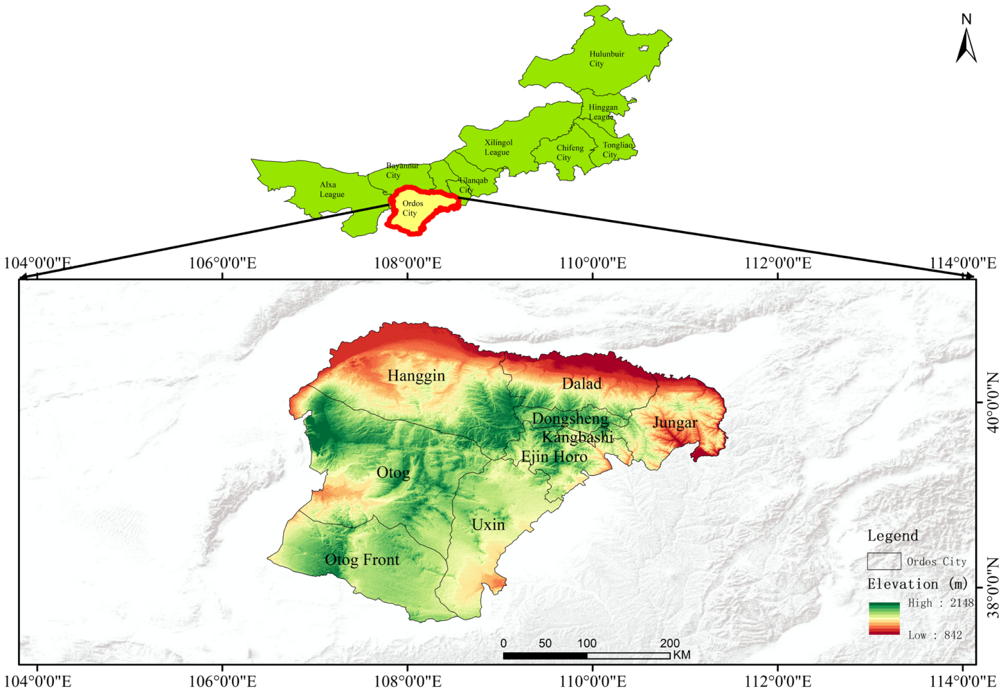
Located in the southwestern part of the Inner Mongolia Autonomous Region, Ordos City covers an area of approximately 86,900 km2. The region is dominated by the Ordos Plateau, with an overall topographical pattern that is elevated in the northwest and lower in the southeast. The area features diverse landform types, primarily including plains, hilly and mountainous regions, undulating plateaus, as well as the Mu Us Sandy Land and the Kubuqi Desert. Among these, the undulating plateaus and sandy lands are widely distributed. The significant variations in surface undulation and substrate characteristics impose critical topographical constraints on the spatial pattern of land use, as illustrated in Figure 1. Furthermore, the Yellow River flows along the northern margin of the study area, supporting a relatively concentrated zone of agricultural and human activities.
The study area features a north temperate semi-arid continental climate, with a multi-year average temperature of 6.2 °C and an average annual precipitation of approximately 348 mm. Precipitation is primarily concentrated between July and September, while annual evaporation significantly exceeds precipitation. Consequently, water availability has become the critical factor constraining ecosystem stability and land use patterns. Under the combined influence of strong winds and an arid climate, the regional ecosystem is highly sensitive to disturbances, facing elevated risks of desertification and soil erosion.
Ordos City is recognized as one of China’s 14 large-scale coal bases, 9 major coal-fired power bases, 5 coal-to-oil and gas bases, and 4 modern coal chemical bases, as well as a crucial gas source for the West-to-East Gas Pipeline Project. The coal industry accounts for half of the city’s industrial economy. Relying on its abundant resource reserves and vital strategic position, Ordos has emerged as a core hub within China’s energy sector. Therefore, the significance of its ecological environment transcends regional boundaries, exerting a profound influence on national energy security, the transformation of resource-based cities, and the green future of the entire industry.
Driven by the combined effects of climatic and geomorphological conditions, the land use types in Ordos exhibit distinct spatial differentiation characteristics, dominated by grasslands, sandy lands, and low-intensity utilized lands. The overall ecosystem is fragile and highly sensitive to human disturbances. In recent years, due to the superimposed effects of climate fluctuations and human activities, regional land use changes have intensified, generating a significant impact on the structure and function of the ecosystem.

2.2. Data Sources and Preprocessing

2.2.1. Data Sources

This study covered six time points from 2000 to 2025, with a five-year interval used as one observation period. The primary data sources are multispectral satellite images. An eight-channel input feature stack combining surface-reflectance and surface-temperature information was constructed to support the discrimination of land-cover classes with similar textures, such as cropland and grassland.
For the 2000–2010 period, 30 m resolution Landsat 5 Level-2 remote sensing imagery was selected, whereas Landsat 8 Level-2 imagery was utilized for the 2015–2025 period [17,19]. These datasets were acquired via the Geospatial Data Cloud and the Google Earth Engine (GEE) platform (Table 2). To reduce seasonal phenological differences, all images were selected within a consistent growing-season window from June 1 to September 30. Images with excessive scene-level cloud contamination were excluded based on the CLOUD_COVER metadata, and cloud and cloud-shadow pixels were further removed using the QA_PIXEL quality assessment band. For each target year, all eligible scenes covering Ordos were composited using a cloud-masked median reducer to generate an annual cloud-reduced mosaic. The resulting mosaics were clipped to the Ordos administrative boundary and exported at a spatial resolution of 30 m for subsequent preprocessing and semantic segmentation.
Thermal information was obtained from the sensor-specific Landsat Collection 2 Level-2 surface-temperature bands, namely ST_B6 for Landsat 5 TM and ST_B10 for Landsat 8 OLI/TIRS. The Level-2 surface-reflectance and surface-temperature products were generated by USGS using its standard processing procedures, including atmospheric correction for the surface-reflectance products. The corresponding Level-2 surface-reflectance and surface-temperature bands were exported from Google Earth Engine in their original scaled integer representation, without applying further scale conversion. According to the product metadata, the surface-reflectance bands have a scale factor of 0.0000275 and an offset of −0.2, whereas the surface-temperature bands have a scale factor of 0.00341802 and an offset of 149.0 K. The Level-2 surface-temperature products for both sensors were provided on a 30 m grid. Therefore, no additional thermal-band resampling was performed before image stacking and patch generation. Although the spectral response functions of Landsat 5 TM and Landsat 8 OLI/TIRS are not identical, all images were processed using the same seasonal compositing window and spatial resolution. No additional cross-sensor radiometric normalization or calibration was applied. The administrative boundary of Ordos City was obtained in GeoJSON format from the National Public Service Platform for Geographic Information and was converted into Shapefile (SHP) format for image clipping and spatial analysis.
In addition, the MODIS Terra Vegetation Indices 16-Day L3 Global 250 m product (MOD13Q1, Collection 6.1) was used as a complementary vegetation-based indicator for the land-cover-based EQI results.

2.2.2. Dataset Generation

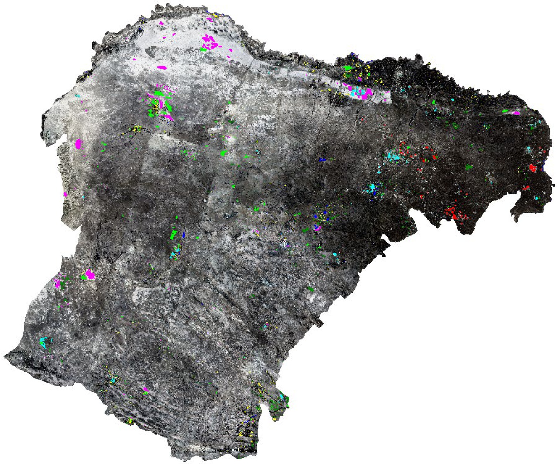
During the sample preparation phase, manual visual interpretation was conducted utilizing remote sensing imagery and auxiliary geographic data to generate pixel-level land use classification labels. To ensure the accuracy and spatial consistency of the annotation results, the generated labels were overlaid onto the original remote sensing imagery for visual assessment, as illustrated in Figure 2. By manually verifying the boundaries of various ground objects and their category distributions, the alignment between the labels and the actual feature characteristics was validated. This procedure helped ensure that the training samples accurately reflect the actual land use conditions within the study area.
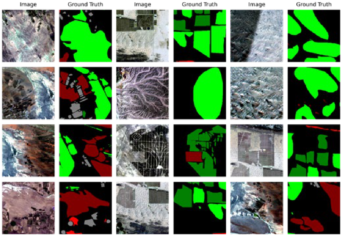
Upon completion of the label generation, a sliding window approach was employed to synchronously crop the original imagery and their corresponding labels into 256 × 256 pixel patches (Figure 3), aiming to construct a dataset suitable for deep learning training. Strict spatial correspondence between the imagery and the labels was maintained during the cropping process, ensuring that each training patch encapsulated complete spatial features and categorical information of the ground objects. To enhance the model’s generalization capability, data augmentation techniques—including random flipping, random rotation, and scale perturbation—were applied to the training samples. These operations were implemented to improve the model’s adaptability to topographical variations, spectral discrepancies, and complex boundary features.
To address the issue of the low proportion of minority classes, such as mining areas, water bodies, and built-up land, priority was given during the cropping process to retain patches that contained a higher proportion of valid labels and richer categorical information. Simultaneously, a class weighting strategy was examined during the preliminary hyperparameter tuning phase to mitigate the adverse impacts of class imbalance on the optimization process and the recognition accuracy of these minority classes. Ultimately, the constructed dataset comprised a training set of 4456 patches (consisting of 1114 original patches and 3342 augmented patches) and a validation set of 254 patches.

3. Theoretical Basis and Methodology

3.1. Research Framework

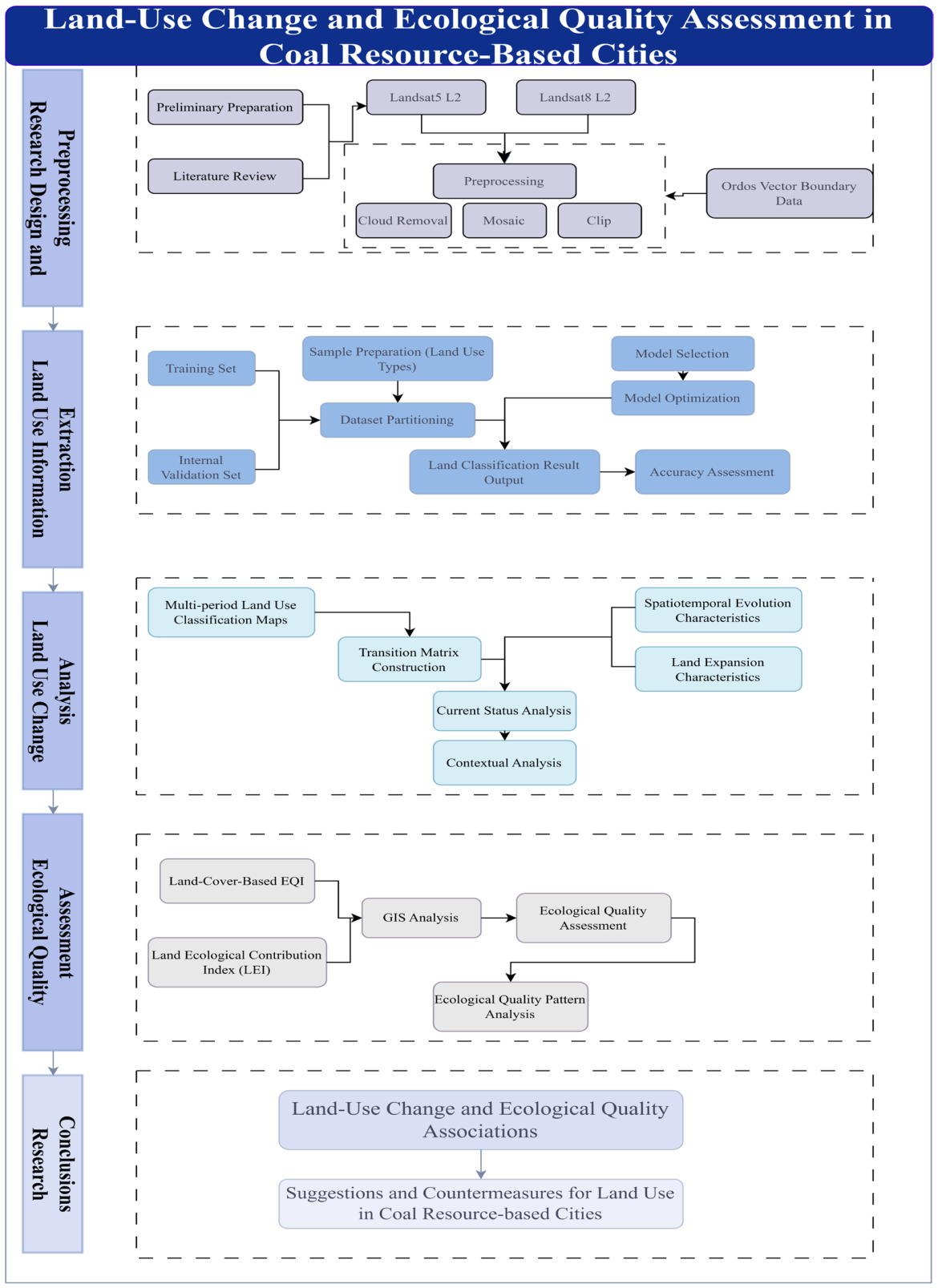
Taking Ordos City as the study area, this research utilizes Landsat series remote sensing imagery from 2000 to 2025 as the primary data source to construct a deep learning-based framework for analyzing land use changes and their land-cover-based ecological quality patterns. Initially, the acquired multi-temporal remote sensing images underwent a series of preprocessing procedures, including cloud removal, mosaicking, and clipping. Subsequently, a land use sample dataset was constructed via manual visual interpretation, integrating high-resolution Google Earth imagery and historical reference data. The U-Net semantic segmentation model was then employed for model training and prediction to generate the multi-temporal spatial distribution data of land use within the study area. The reliability of the classification results was rigorously verified through accuracy assessment metrics [46].
Based on these results, a land use transition matrix was utilized to analyze the conversion relationships among various land cover types and the evolutionary characteristics of land use patterns. Emphasis was placed on identifying the dynamic trajectories of principal land categories, including grassland, unused land, mining areas, and built-up land. Furthermore, EQI and LEI were combined to quantitatively characterize the associations between land-use dynamics and land-cover-based ecological quality patterns [42]. GIS spatial analysis was also used to examine spatial and temporal variations in land-cover-based ecological quality. These findings aim to provide a robust scientific foundation for territorial spatial optimization and eco-environmental governance in Ordos City and other similar resource-based cities. The overall research framework is illustrated in Figure 4.

3.2. Methodology

Before analyzing land-use change and its land-cover-based ecological quality patterns, the quality of the classification dataset was evaluated. The experiments were implemented using the PyTorch (version 2.0.1) deep learning framework and the MMSegmentation (version 1.2.2) toolbox, performing pixel-wise semantic segmentation on the Landsat series remote sensing imagery of Ordos City at five-year intervals from 2000 to 2025. Compared with traditional machine learning methods, the U-Net semantic segmentation architecture demonstrates significant advantages in processing fragmented surfaces in mining areas and distinguishing highly similar ground objects, such as open-pit mines and bare land. To ensure the reliability of the ecological quality patterns analysis, a semantic segmentation dataset comprising seven typical land cover categories (mining areas, water bodies, cropland, grassland, forest land, built-up land, and unused land) was constructed through manual annotation and patch cropping.
To construct a high-quality semantic segmentation dataset optimized for deep learning, a sliding window strategy was adopted to crop the original large-format multispectral images. Each patch was 256 × 256 pixels and retained all eight channels of the input feature stack. In contrast to conventional three-channel RGB datasets, this dataset was not subjected to dimensionality reduction, thereby providing the model with richer spectral features to differentiate similar ground objects. During the training phase, the model directly accepted tensor inputs of 256 × 256 × 8, which avoided interpolation errors and information loss caused by image resizing.
  • Land Use Transition Matrix:
The land use transition matrix is utilized to reflect the dynamic processes of mutual conversion among different land cover areas within the study region during the research period, as expressed in (1) [12]:
A i j = A 11 A 12 A 1 n A 21 A 22 A 2 n A n 1 A n 2 A n n
where A i j   denotes the area converted from land-use type i at the beginning of the study period to land-use type j at the end of the study period; and n is the total number of land-use types, with i , j = 1,2 , , n .
  • Ecological Environmental Quality Index:
The ecological environmental quality index (EQI) was used to characterize land-cover-based ecological quality patterns of the study area and was calculated using Equation (2) [47,48].
E Q I t = i = 1 n A t i × R i / T A t
where E Q I t denotes the ecological environmental quality index at time t ; A t i denotes the area of the i -th land-use type at time t ; R i   denotes the ecological quality coefficient assigned to the i -th land-use type; T A t denotes the total area of the study area at time t ; and n denotes the total number of land-use types.
Conventional EQI assessments generally merge built-up land and mining areas into a single category, both assigned a value of 0.20. Considering that the study area is characterized by intensive coal mining activities, the ecological disturbance caused by open-pit mining, waste dump occupation, and land subsidence is substantially greater than that associated with built-up land. Therefore, to more accurately quantify the mining-related land-cover change by this specific land-use type, the classification scheme was further refined in this study. Based on existing ecological quality assessment frameworks and expert knowledge of coal mining environments, the weight values were adjusted to better reflect relative ecological impacts. Built-up land was assigned a value of 0.20, while mining areas were assigned a slightly lower value of 0.18 to represent the greater ecological disturbance associated with mining areas. This adjustment does not alter the structure of the EQI model but refines parameterization to improve its sensitivity to mining-related land-cover change in the study area, as shown in Table 3 [4,49].
In this study, EQI is used as a land-cover-based ecological proxy derived from land-cover areas and predefined ecological quality coefficients. It describes ecological quality patterns associated with land-cover composition. Based on the predefined ecological quality coefficients and the land-use transition matrix, LEI was used to quantify the relative contribution of each transition type to the overall change in EQI. It helps identify major land-use transitions associated with increases or decreases in this proxy indicator, but cannot serve as a direct measure of ecological change or as evidence of a causal ecological effect.
The MODIS Normalized Difference Vegetation Index (NDVI) was used as a complementary vegetation-based indicator for the land-cover-based EQI results. Specifically, the MODIS Terra Vegetation Indices 16-Day L3 Global 250 m product was selected to calculate the growing-season mean NDVI for each target year. To keep the NDVI analysis consistent with the Landsat compositing period, MODIS images from June 1 to September 30 were used for 2000, 2005, 2010, 2015, 2020, and 2025. The NDVI band was scaled by 0.0001, clipped to the Ordos administrative boundary, and averaged to obtain the annual growing-season mean NDVI. This MODIS-derived NDVI was not involved in land-use classification, EQI calculation, or LEI calculation, and was used only as a complementary indicator of vegetation change.
  • Ecological contribution index (LEI):
The LEI quantifies the relative ecological contribution associated with a specific land-use transition, as calculated in (3):
L E I = R 1 R 0 × L A T A
where L E I denotes the ecological contribution index; R 0 and R 1   denote the ecological quality index values of the corresponding land-use types at the beginning and the end of the study period, respectively; L A denotes the area of the corresponding land-use transition; and T A denotes the total area of the study area [12].
  • Accuracy Assessment:
To objectively evaluate the performance of the proposed classification framework, the ESA WorldCover dataset was introduced as a benchmark for comparison [14,50]. To ensure the consistency of data processing, the 11 original land-cover classes defined in the dataset were first mapped and reclassified according to their corresponding categories, and then aggregated into the six target land-cover categories used for comparison; mining areas were excluded because ESA WorldCover does not provide a separate mining category. This process ensured consistency in both land-cover classification and subsequent analyses within the study area. A stratified random sampling strategy was subsequently adopted. Specifically, 100 validation samples were randomly selected from each of the seven land-cover categories, namely unused land, water bodies, cropland, mining areas, forest land, built-up land, and grassland, resulting in a total of 700 validation points. These points were randomly selected from locations outside the training and fine-tuning regions based on their recorded spatial coordinates, ensuring that the independent validation points did not spatially overlap with the samples used for model training or fine-tuning. No fixed minimum-distance buffer was applied. Visual interpretation results were used as the reference data, and the classification performance of the proposed model was quantitatively compared with that of the ESA WorldCover product. The independent validation points were not used for model training, fine-tuning, or internal validation. This design was adopted to reduce potential overestimation of map-level accuracy.

3.3. Improved U-Net Semantic Segmentation Network

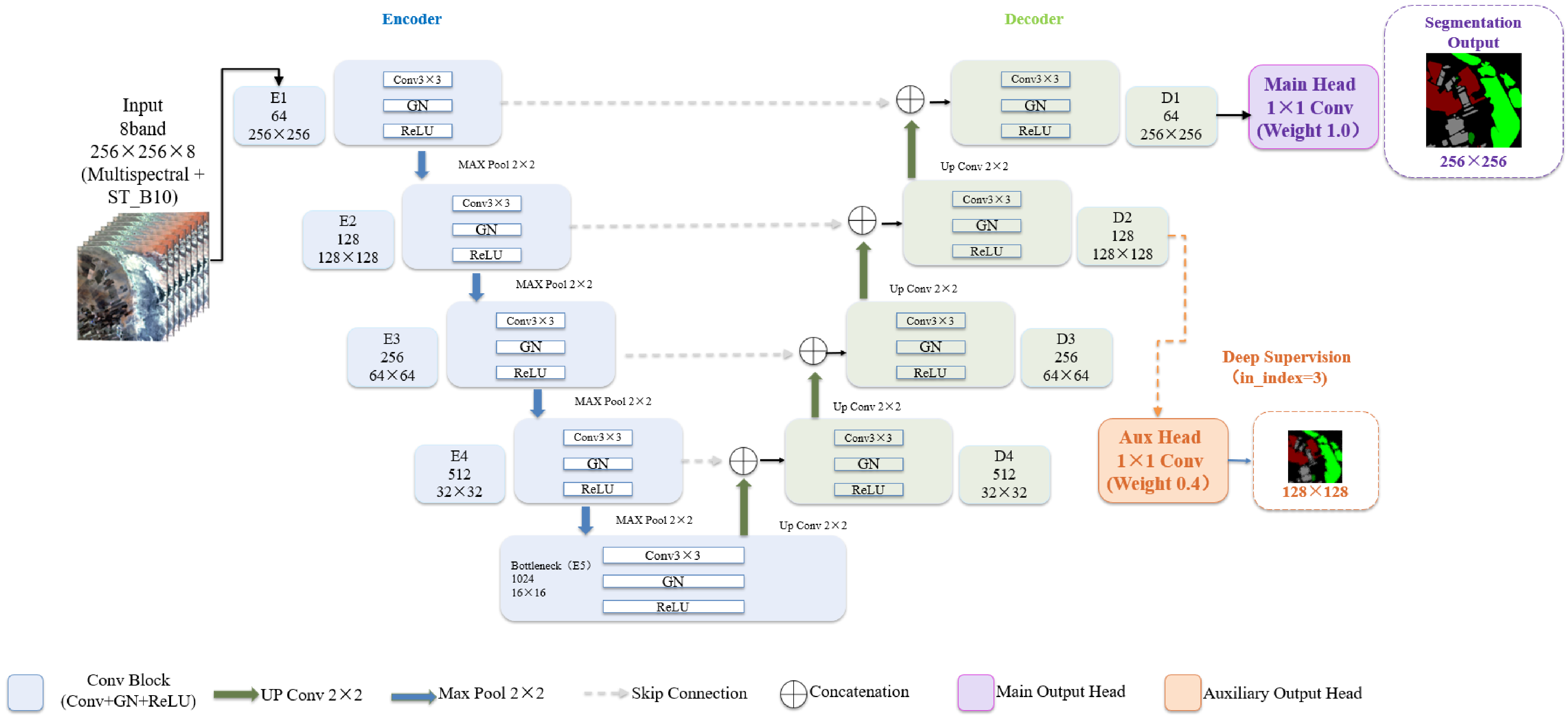
Considering the complex land surface characteristics of mining areas and the unique geomorphological conditions of arid regions, the conventional U-Net model exhibits certain limitations in fine-grained feature extraction and multi-scale boundary segmentation [39,51]. To address these limitations, an improved U-Net-based semantic segmentation model incorporating multiple optimization strategies was developed in this study. The overall architecture of the proposed network is shown in Figure 5.
The proposed model takes an eight-channel input feature stack and generates pixel-wise classification results for seven land-use categories. During the encoding stage, hierarchical feature representations with 64, 128, 256, and 512 channels are progressively extracted, while the bottleneck layer further enlarges the receptive field. During the decoding stage, feature maps are progressively upsampled and concatenated with the corresponding encoder features through skip connections [32,52]. Finally, a (1 × 1) convolution is employed to produce the class probability for each pixel. Based on the conventional U-Net architecture, the proposed model was comprehensively improved from four aspects, namely data input, network architecture, supervision strategy, and loss function.

3.3.1. Multispectral and Thermal Feature Fusion Input

When processing surface imagery of semi-arid coal resource-based cities, conventional 3-channel RGB visible light data exhibit severe limitations in information dimensionality. Due to sparse surface vegetation and intensive open-pit mining activities, the study area is highly susceptible to spectral confusion—specifically, different ground objects exhibiting similar spectral signatures or identical objects displaying varying spectra, which leads to severe model misclassifications. To address this issue, this study overcomes the constraints of traditional three-channel inputs by constructing an eight-channel high-dimensional feature space, comprising corresponding optical reflectance channels and sensor-specific thermal information as the network input. The introduction of surface temperature features provides the U-Net model with supplementary thermodynamic physical information beyond optical reflectance. This helps improve the model’s capability to decouple features and distinguish mining areas from natural sandy land and fallow farmland, thereby effectively improving the segmentation accuracy. To construct a consistent eight-channel input feature stack across Landsat 5 TM and Landsat 8 OLI/TIRS imagery, the bands were aligned according to their spectral or physical meanings rather than their original band numbers. For Landsat 8 OLI/TIRS, seven surface reflectance bands (SR_B1–SR_B7) and the land surface temperature band (ST_B10) were selected. For Landsat 5 TM, the corresponding blue, green, red, near-infrared, shortwave-infrared 1, shortwave-infrared 2, and thermal channels were represented by SR_B1, SR_B2, SR_B3, SR_B4, SR_B5, SR_B7, and ST_B6, respectively (Table 4). Because Landsat 5 TM does not include a coastal aerosol band equivalent to Landsat 8 OLI SR_B1, Landsat 5 SR_B1 was repeated as an auxiliary channel to preserve the same input dimensionality required by the segmentation network. This duplicated channel was used only for input-dimensional consistency and was not interpreted as an independent spectral band. The eight input channels were constructed from the Level-2 surface-reflectance bands and the sensor-specific surface-temperature band after export to a common 30 m grid.

3.3.2. Group Normalization-Based Underlying Architecture Reconstruction

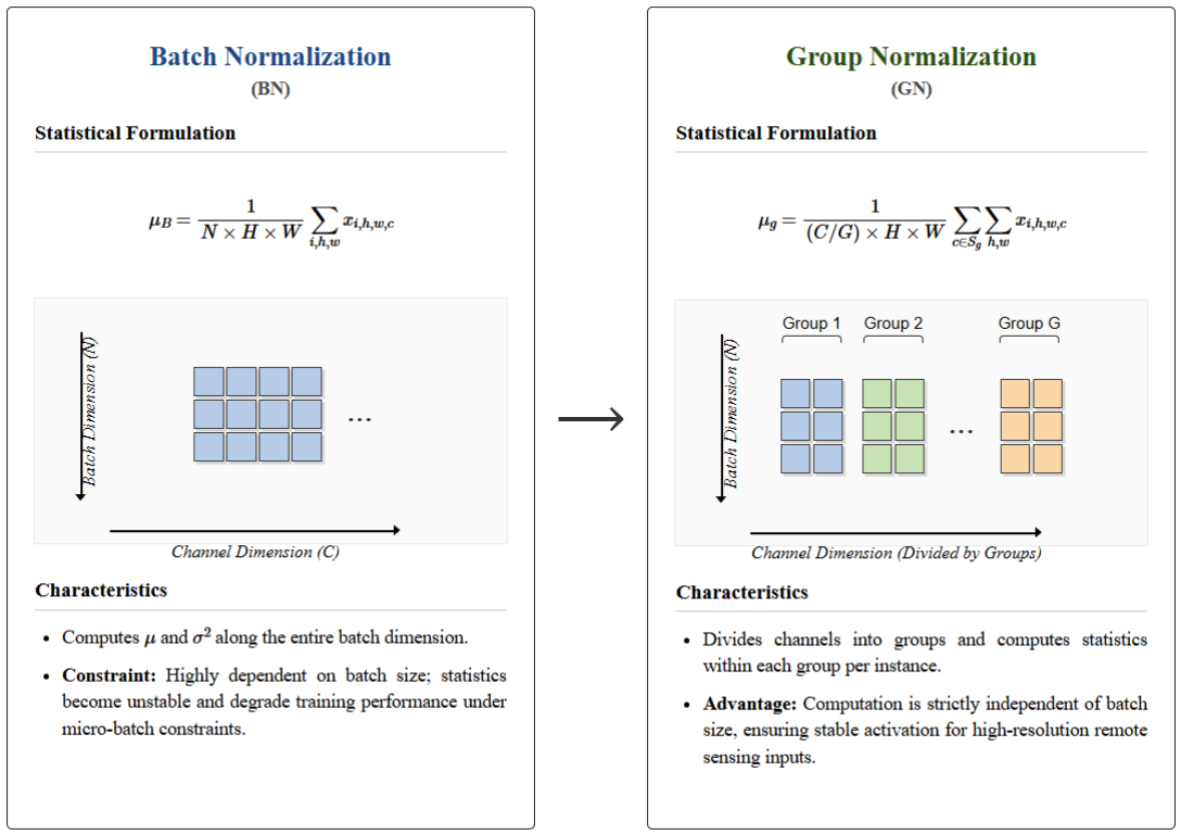
The conventional U-Net architecture heavily relies on batch normalization (BN) layers to accelerate convergence. However, due to the introduction of eight-channel input features in this study, the memory consumption of each remote sensing patch increases significantly, resulting in a strict limitation on the batch size during training. Under extremely small batch-size conditions, the statistical estimation of mean and variance in BN becomes unstable due to insufficient samples, which may lead to severe fluctuations and degrade the stability of feature representation as well as the generalization capability of the model.
To address this issue, the activation module in the shallow layers of the network was redesigned, as shown in Figure 6 [53]. Specifically, BN layers were completely removed and replaced with group normalization (GN). Unlike BN, which performs normalization across the batch dimension, GN divides the channels of a single sample into groups and performs normalization independently within each group. The improved basic convolutional block is composed of a sequential combination of convolution, GN, and ReLU activation. This design decouples the normalization process from the batch size, enabling stable and robust feature learning under limited memory conditions.

3.3.3. Deep Supervision Mechanism for Alleviating the Vanishing Gradient Problem

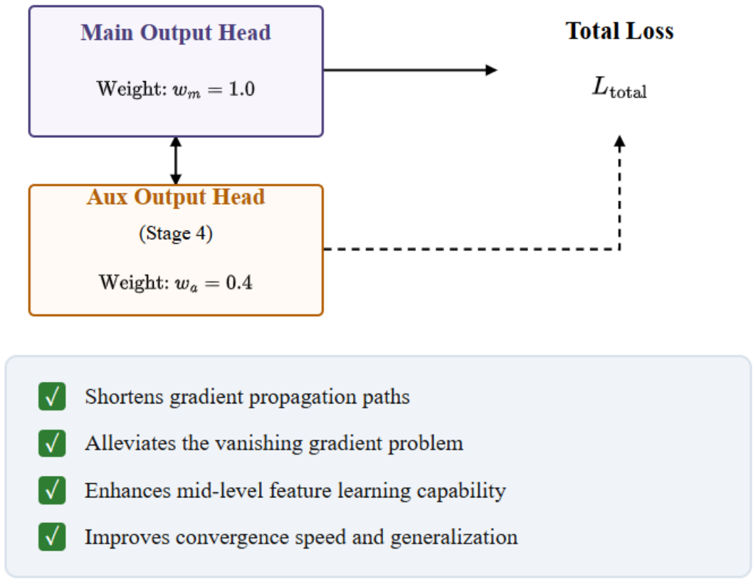
In deep encoder–decoder architectures, error signals are prone to exponential decay during backpropagation over long paths [54]. This causes delayed weight updates in the shallowest encoder layers—the classic vanishing gradient problem—which can be problematic for complex geospatial feature extraction. To maintain highly efficient backpropagation, we introduce a Deep Supervision (DS) mechanism at the fourth stage of the U-Net decoder (the deep feature map at in_index = 3), as depicted in Figure 7. Specifically, a dedicated auxiliary decoding head is added alongside the main output head, with a weight coefficient set to 0.4. By deploying auxiliary supervision branches at various hierarchical levels, the network imposes explicit constraints on intermediate representations, allowing the supervisory signals to help guide the joint optimization of shallow and deep features. Consequently, the DS strategy can alleviate information degradation during gradient flow, improving training stability and convergence behavior, while also enriching the model’s representation of complex spatial features [32,55].

3.3.4. OHEM-Based Hard Pixel Mining Strategy

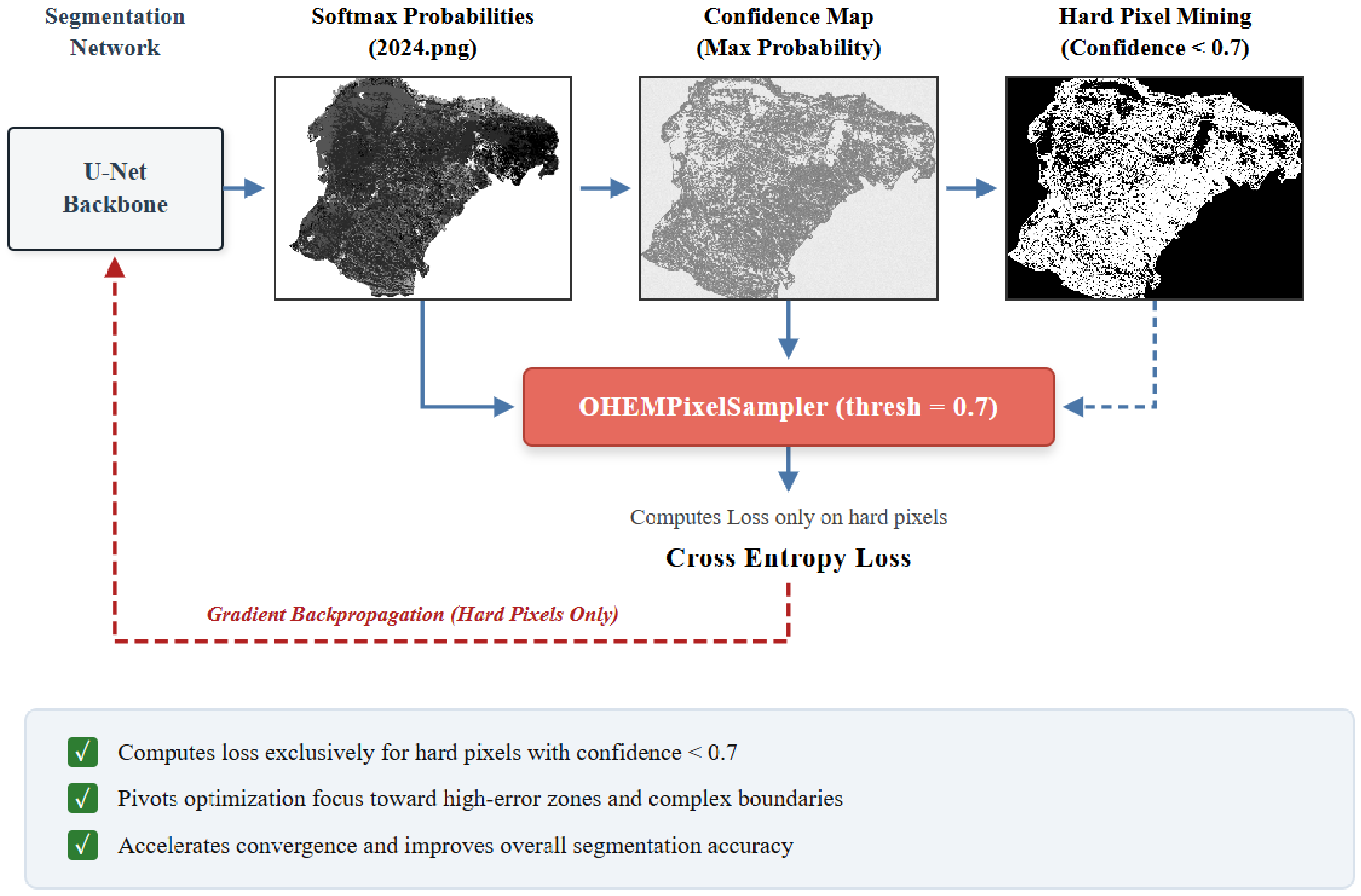
Standard cross-entropy loss assigns equal weight to every pixel. Nevertheless, in large-scale land cover classification, remote sensing imagery is typically dominated by homogeneous regions with simple, easily recognizable textures. These straightforward samples constitute a disproportionate share of the loss and can easily overwhelm the parameter optimization process. Consequently, the network pays insufficient attention to challenging samples, such as fragmented patches in mining areas, transitional zones between land covers, and complex boundaries. To improve the model’s proficiency in handling challenging regions, we integrate the Online Hard Example Mining (OHEM) mechanism into the network’s output stage (Figure 8). Before computing the loss, OHEM dynamically filters the pixels based on their prediction confidence. It discards high-confidence “easy” pixels and retains only the “hard” pixels for loss calculation and backpropagation. By pivoting the optimization focus toward high-error zones and complex boundaries, OHEM shifts the network’s ability to capture fine-grained spatial representations, elevates the classification accuracy of complex ground objects, and mitigates commission and omission errors [56,57].

3.3.5. Model Implementation and Training Settings

The experiments were conducted on a Dell Precision 7920 Tower workstation (Dell Technologies Inc., Round Rock, TX, USA) equipped with an NVIDIA RTX A5000 GPU (NVIDIA Corp., Santa Clara, CA, USA). The proposed model was implemented using the EncoderDecoder framework in MMSegmentation. The backbone adopts a U-Net architecture with five encoder–decoder stages, eight input channels, and 64 base channels. Group normalization with four groups was used after convolution to replace batch normalization under the limited batch-size setting. The main decode head was implemented as an FCN head to output seven land-cover classes. An auxiliary FCN head with a loss weight of 0.4 was introduced at an intermediate decoder stage for deep supervision. OHEM was applied in the main decode head with a confidence threshold of 0.7 and a minimum retained pixel number of 10,000. The training batch size was 16, and the internal-validation batch size was 1. Class weighting was examined during preliminary hyperparameter tuning. The weights were specified with reference to the proportions of labeled pixels in the seven land-cover classes. The candidate weights were set empirically with reference to these relative proportions rather than calculated using a fixed formula. Following the class order used in the model configuration, namely cropland, grassland, unused land, water bodies, built-up land, forest land, and mining, the tested class weights were 1.5, 1.5, 1.2, 1.0, 1.0, 1.0, and 1.5, respectively. The same weights were applied to both the main and auxiliary decode heads during these preliminary experiments. Class weighting was used only during preliminary hyperparameter tuning and was not included in the final model configuration. Therefore, the model used for the reported results, including an internal-validation mIoU of 69.51%, was trained with unweighted cross-entropy loss. The loss weights of the main and auxiliary heads were 1.0 and 0.4, respectively. The model was trained with the AdamW optimizer using a learning rate of 5 × 10⁻⁶ and a weight decay of 0.01. A polynomial learning-rate schedule was adopted, and the maximum number of training iterations was set to 15,000, with validation performed every 500 iterations. During inference, full-coverage prediction was generated using a sliding-window strategy with a crop size of 256 × 256 and a stride of 170 × 170. The same training settings were used for the comparison models unless otherwise specified.

3.4. Spatiotemporal Transfer and Fine-Tuning Strategy

In this study, a spatiotemporal transfer and fine-tuning strategy was adopted to improve the adaptability of the classification model across different years and Landsat sensors [23,58]. The model was first trained using labeled samples from the 2025 source period. The resulting model was directly applied to the Landsat 8 images from 2020 and 2015. To improve its adaptation to the Landsat 5 data, additional image-label patches were manually interpreted from the 2010 Landsat composite image and added to the training set for fine-tuning. The checkpoint obtained after the 2010 fine-tuning stage was then used to classify the Landsat images from 2005 and 2000. These samples were mainly collected from land-cover types with large spectral variations or high confusion, such as mining areas, built-up land, unused land, and grassland.
After these samples were added, the fine-tuning set included 248 image and label patch pairs, and 172 patch pairs were used for internal validation during training. Each image patch was 256 × 256 pixels with eight input channels and was paired with a corresponding land-cover label. The fine-tuning samples covered all seven land-cover classes, with cropland and mining areas accounting for the largest proportions of labeled pixels. The model was initialized with the checkpoint obtained from the 2025 source-period training, and all network parameters were updated during fine-tuning. The optimizer, learning rate schedule, batch size, validation interval, and maximum number of iterations were kept the same as in the initial training stage.

4. Results and Analysis

4.1. Training Results and Accuracy Assessment

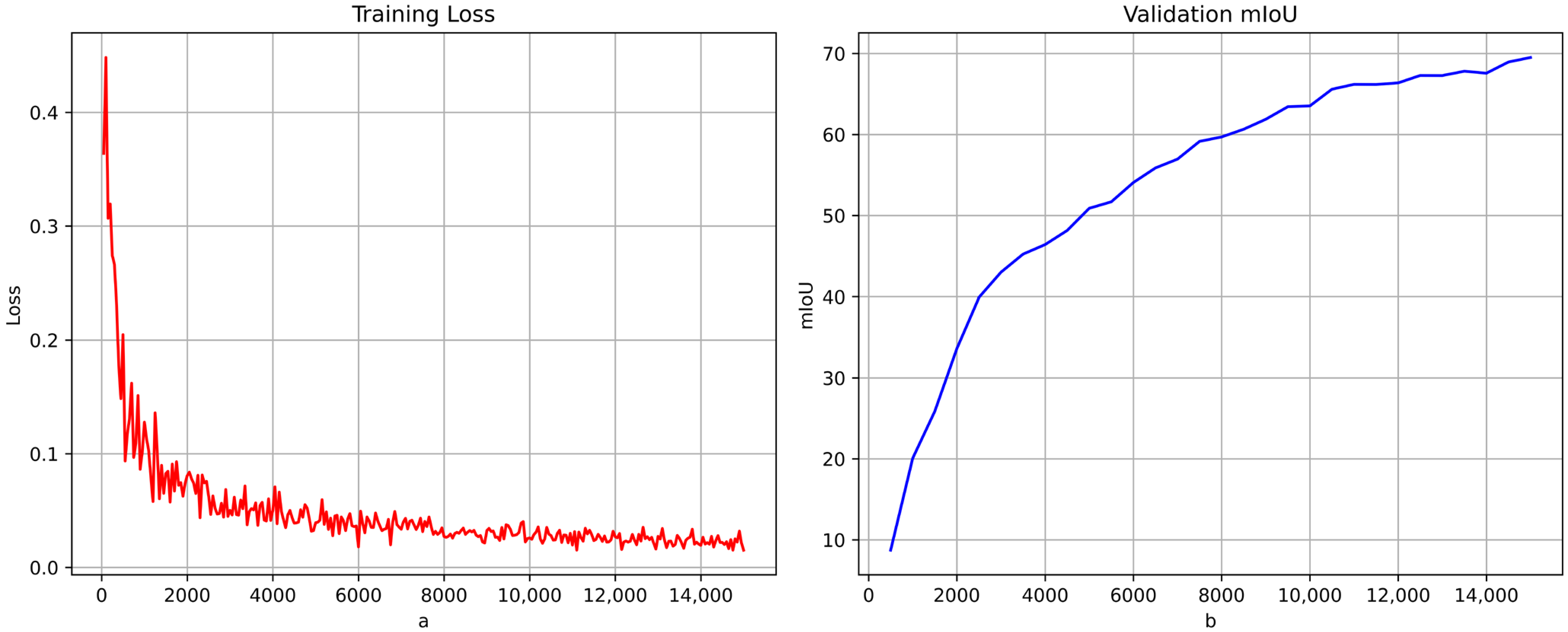
The proposed model was implemented and trained utilizing the PyTorch and MMSegmentation frameworks. Model convergence was continuously monitored using the mean Intersection over Union (mIoU) and loss metrics, supplemented by qualitative evaluations of visualizations from the validation set. During preliminary model development, iterative refinements to the training samples and optimization settings, including image patching, data augmentation, and learning-rate tuning, were associated with improved segmentation accuracy. Visually, the model showed reasonable recognition performance for primary land-cover types (e.g., grassland, forest, cropland, and water bodies) as well as complex classes like mining areas and built-up land. Nevertheless, constrained by image spatial resolution and the mixed pixel effect, some misclassifications remain in challenging areas, particularly along mining boundaries and the transitional zones between bare land and built-up areas. No additional spatial post-processing or manual correction was applied to the final land-cover maps used in the subsequent analyses. The corresponding training dynamic curves are illustrated in Figure 9.
Table 5 presents the classification accuracy evaluation results for various land use types. In terms of overall performance, the model achieves an overall accuracy (aAcc) of 83.16%, a mean accuracy (mAcc) of 81.65%, and a mean Intersection over Union (mIoU) of 69.51%. These metrics demonstrate that the proposed model effectively accomplishes the land use classification task in the study area and shows useful feature recognition capability under the internal validation setting.
Analyzing the class-specific results, Cropland yielded the highest classification accuracy, with its IoU and Class Acc reaching 89.20% and 92.48%, respectively. This is primarily attributed to the widespread distribution and strong spatial continuity of cropland within the study area, coupled with its relatively stable textural and spectral characteristics, which enable the model to effectively learn its spatial distribution patterns. Grassland also attains a high accuracy, recording an IoU of 80.28% and a Class Acc of 91.22%, indicating the model’s proficiency in identifying vegetation-covered regions.
The mining area class achieved an IoU of 69.61% and a Class Acc of 88.72%, ranking among the best-performing categories. These results indicate that the proposed model can effectively capture characteristic features of mining areas, including exposed surfaces, mining-induced disturbances, and terrain variations, thereby supporting the identification of mining area boundaries. Nevertheless, some confusion remains along boundary regions, where the spectral and spatial characteristics of adjacent bare land and built-up land are similar, resulting in occasional misclassification.
The unused land class obtained an IoU of 65.77% and a Class Acc of 78.85%, representing moderate classification performance. The relatively heterogeneous surface conditions within this class, together with its spectral and textural similarities to exposed mining surfaces and built-up land in certain regions, increase the difficulty of class discrimination and consequently reduce the classification accuracy.
The water body and built-up land classes achieved IoU values of 62.51% and 60.88%, respectively. Although both classes were identified with satisfactory overall performance, misclassification still occurred in some areas due to the effects of spatial resolution limitations and mixed pixels. In particular, errors were mainly observed along the boundaries of small water bodies and at the interfaces between built-up land and bare surfaces. The forest class had the lowest IoU among all categories (58.32%), with a Class Acc of 72.81% This relatively lower performance may be attributed to both the limited quantity and quality of forest training samples and the spectral similarity between forest, grassland, and cropland, all of which are vegetation-covered land cover types. These similarities increase the difficulty of class discrimination and lead to confusion during classification. Moreover, small and fragmented forest patches are more susceptible to mixed pixel and boundary effects, further reducing the classification accuracy.
It is worth noting that the water body, built-up land, and forest classes all exhibited higher Class Acc than IoU values. This observation suggests that the proposed model can reliably identify the dominant regions of these classes, while most classification errors are concentrated along object boundaries and transition zones. Overall, the results demonstrate that the proposed model showed useful land-cover discrimination capability under the internal validation setting. The remaining classification errors are primarily associated with complex boundary regions and small fragmented patches rather than large-scale misclassification among different land cover classes.
Image preprocessing was found to influence classification performance. The original mosaicked images exhibited radiometric differences among scenes, including variations in color and brightness, resulting in unstable spectral responses for the same land-cover class. To mitigate this issue, cloud masking and annual median mosaicking were applied consistently on the Google Earth Engine (GEE) platform to reduce cloud contamination and visual discontinuities among scenes within each annual mosaic.
To improve the model’s spatiotemporal generalization capability, spatiotemporal transfer learning was further investigated. Owing to differences in sensor characteristics, climatic conditions, and land surface phenology, the spectral signatures of identical land-cover classes vary considerably across acquisition periods. For example, the near-infrared reflectance of grassland and cropland differs markedly between dry and wet years, increasing the difficulty of cross-temporal classification. As described in Section 3.4, the 2025 source-period model was fine-tuned using supplementary samples from the 2010 Landsat 5 composite image to improve its adaptation to Landsat 5 imagery. The resulting checkpoint was subsequently used to classify the 2005 and 2000 Landsat images. Figure 10 shows the visual comparison between the predicted classification maps and the reference labels. The visual comparison suggests that the predicted maps generally preserve the spatial distribution of major land-cover classes and are broadly consistent with the reference annotations.

4.2. Model Performance Evaluation

4.2.1. Ablation Study

To evaluate the contribution of each proposed module to complex land-cover classification, a series of ablation studies was conducted under identical experimental settings, including the same dataset, training strategy, and hyperparameter configuration. The quantitative ablation results are summarized in Table 6 and Table 7, and the evolution of the validation mIoU during training is presented in Figure 11.
Compared with the baseline U-Net, the introduction of GN increased the mIoU from 45.99% to 61.33%, indicating improved optimization stability under the small-batch training setting. After adding auxiliary supervision, the mIoU further increased to 69.25%, suggesting that auxiliary supervision facilitated gradient propagation and deep feature learning. The final model with OHEM achieved the highest aAcc of 83.16% and mIoU of 69.51%.
The class-level results further show that the baseline U-Net failed to effectively identify grassland and water bodies, with IoU values of 0.00% for both classes. After GN was introduced, the IoU values of grassland and water bodies increased to 55.84% and 58.54%, respectively. Auxiliary supervision further improved the recognition of grassland, water bodies, forest, and mining areas. Although OHEM produced only a marginal improvement in overall mIoU compared with the GN + auxiliary supervision model, it increased the IoU of mining areas from 64.02% to 69.61% and that of unused land from 59.73% to 65.77%, indicating that OHEM mainly contributed to the discrimination of difficult and spectrally confused classes.
The validation mIoU curves in Figure 11 are consistent with the quantitative results. The baseline U-Net reached a low plateau, and the GN-based model still fluctuated during later iterations. The model with auxiliary supervision achieved higher mIoU but retained several abrupt drops. By comparison, the final model with OHEM showed a smoother upward trend and remained more stable after about 10,000 iterations. This indicates that OHEM contributed to later-stage optimization stability and improved the recognition of difficult classes such as mining areas and unused land.
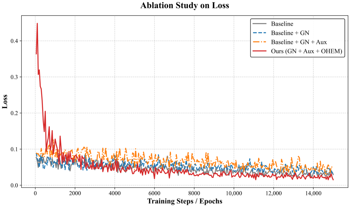
As shown in Figure 12, the training loss of all model variants decreases progressively, indicating that each model converges during the optimization process. Compared with the other configurations, the proposed model exhibits a relatively higher loss at the beginning of training because OHEM places greater emphasis on difficult samples, particularly ambiguous boundary pixels, resulting in a larger initial optimization objective. As training proceeds, however, the loss decreases more rapidly and gradually converges to the lowest value among all compared models. This observation indicates that the proposed combination of GN, auxiliary supervision, and OHEM not only improves optimization stability but also facilitates more effective convergence. Consequently, the model achieves better convergence behavior in this experiment, which is consistent with the improved classification accuracy observed on the validation set.

4.2.2. Comparison with Baseline Segmentation Models

To further evaluate the proposed framework, U-Net, ResUNet, DeepLabV3+, FCN, PSPNet, and SegNet were selected as baseline models and trained under the same data split, input bands, and evaluation protocol. As shown in Table 8, several baseline models achieved higher overall mIoU than the proposed model, with SegNet obtaining the highest mIoU of 75.11%. However, the proposed model achieved the highest IoU for mining areas, reaching 69.61%. This result indicates that the main advantage of the proposed framework lies in recognition of mining areas, which is the key classification target for the subsequent land-use transition and ecological quality analyses.
To examine the robustness of the proposed model under different random initializations, random-seed experiments were conducted. The final model used in this study is also reported for reference. As shown in Table 9, the repeated runs showed limited variation in overall performance, with an mIoU of 68.97 ± 0.20%. The Mining IoU reached 69.00 ± 0.62%, indicating that the proposed model maintained relatively stable performance for the target mining category.

4.2.3. Computational Complexity Analysis

In this study, computational complexity was further analyzed for the proposed U-Net-based framework. Since the proposed model was constructed on the basis of U-Net, the comparison focused on the U-Net baseline, its ablation configurations, and ResUNet as a related U-Net-based model. The number of parameters and GFLOPs were calculated under the same input setting, using a single eight-channel image patch with a spatial size of 256 × 256 pixels. The results are shown in Table 10.
The proposed model has nearly the same parameter number as the baseline U-Net and only a slight increase in GFLOPs, from 49.11 to 49.23. This is because Group Normalization mainly replaces Batch Normalization, while auxiliary supervision and OHEM are training-stage strategies and do not substantially increase the inference-stage network structure. Compared with the baseline U-Net, the proposed model improves the mIoU from 45.99% to 69.51% under a similar computational cost. Compared with ResUNet, the proposed model requires fewer parameters and lower GFLOPs while achieving higher mIoU. These results indicate that the proposed configuration improves mining areas recognition with only a slight increase in computational complexity compared with the baseline U-Net.
4.3. Land Cover Classification Results and Spatiotemporal Analysis

4.3.1. Multi-Temporal Land Cover Classification Results

Based on the trained proposed U-Net model, land cover classification maps of Ordos for 2000, 2005, 2010, 2015, 2020, and 2025 were generated, as shown in Figure 13. The classification results indicate that grassland, unused land, and forest constitute the dominant land cover types across the study area, whereas water bodies occupy only a relatively small proportion. Although mining areas and built-up land account for a comparatively limited area, they exhibit pronounced spatiotemporal dynamics and therefore serve as important indicators of human-induced land surface disturbance.
From the spatial distribution patterns, grassland and unused land are widely distributed across the Ordos Plateau and surrounding sandy regions. Forest is primarily concentrated in areas associated with ecological restoration, vegetation rehabilitation, and favorable local topographic and hydrological conditions. Built-up land is mainly distributed around urban areas and transportation corridors, whereas mining areas are closely associated with coal resource exploitation and exhibit fragmented spatial patterns with intensive local disturbances.

4.3.2. Accuracy Assessment

The evaluation results (Table 11) indicate that the proposed model achieves an overall accuracy (OA) of 66.00% and a Kappa coefficient of 0.6033, outperforming the ESA WorldCover product, which attains an OA of 48.71% and a Kappa coefficient of 0.4020. In comparison, the proposed model improves OA by 17.29 percentage points and Kappa by 0.2013, demonstrating enhanced classification reliability in complex mining-dominated landscapes.
It should be noted that the accuracy metrics reported in Table 5 and Table 11 are based on different validation protocols. Table 5 reports the internal semantic segmentation validation results calculated from held-out image patches, where mIoU is used as the primary metric for evaluating multi-class segmentation performance. In this internal validation, the proposed model achieved an mIoU of 69.51%, a mean accuracy (mAcc) of 81.65%, and a pixel-level overall accuracy (aAcc) of 83.16%. In contrast, Table 11 reports an independent map-level accuracy assessment based on 700 stratified random validation points, with 100 points selected for each land-cover class. Therefore, the OA of 66.00% in Table 11 reflects the external point-based accuracy of the final land-cover map, rather than the internal patch-based model validation accuracy. The difference between these values is mainly related to the different sampling units, evaluation protocols, mixed-pixel effects, boundary uncertainty, and the spectral confusion among mining areas, built-up land, unused land, and grassland.
From a class-wise perspective, higher F1-scores are observed for unused land, water bodies, and cropland. Specifically, unused land achieves an F1-score of 83.04%, followed by water bodies (80.00%) and cropland (76.92%), indicating that the model can effectively delineate dominant land cover types in the study area.
For the mining area class, the proposed model achieves a producer’s accuracy (PA) of 60.00%, a user’s accuracy (UA) of 80.00%, and an F1-score of 68.57%. In contrast, ESA WorldCover does not include a dedicated mining class; therefore, mining pixels cannot be properly represented, resulting in an F1-score of 0 for this category. This highlights the advantage of introducing an independent mining class for capturing anthropogenic disturbance associated with extraction activities.
For built-up land and grassland, the proposed model achieves F1-scores of 56.10% and 57.72%, respectively, representing improvements of 12.82 and 20.18 percentage points over ESA WorldCover. These improvements suggest that the proposed model is more effective in distinguishing spectrally similar land cover types, particularly in areas where built-up land, grassland, and mining surfaces exhibit overlapping spectral characteristics.
The forest class yields a relatively lower F1-score of 40.66%. Confusion matrix analysis indicates that a portion of forest samples is misclassified as grassland. This misclassification is primarily attributed to the ecological characteristics of the arid and semi-arid study area, where forest is dominated by sparse woodland and shrubland. These vegetation types exhibit similar spectral responses to natural grassland, leading to reduced separability between the two classes.
Overall, the ESA WorldCover product demonstrates relatively reliable performance in large-scale land cover mapping, particularly for spectrally stable classes such as water bodies and cropland, where higher classification accuracies are observed. However, its performance is less satisfactory in complex mining-dominated regions, where both the classification scheme and spatial representation capability appear to be limited under heterogeneous surface conditions.
These results suggest that, for resource-based cities characterized by intensive anthropogenic disturbance and fragmented land cover patterns, region-adaptive and fine-grained land use/land cover (LULC) classification approaches remain necessary to better capture local spatial heterogeneity.

4.3.3. Area Change Characteristics of Different Land Cover Classes

The areas of different land cover classes were calculated from the multi-temporal classification maps, and the statistical results are summarized in Table 12. Based on these results, the temporal variations in the area of each land cover class were further analyzed. The changes observed between 2010 and 2015 should be interpreted with caution because this interval coincides with the transition from Landsat 5 TM to Landsat 8 OLI/TIRS. Although all images were processed using a consistent growing-season compositing window and a 30 m spatial resolution, residual cross-sensor differences may affect the temporal comparability of the mapped class areas. Therefore, the observed changes during this interval may reflect both actual land-cover transitions and residual sensor-related uncertainty.
From 2000 to 2025, grassland consistently represents the dominant land cover type in the study area, increasing from 42,222.55 km2 to 44,880.41 km2, and maintaining a high proportion throughout the study period, indicating its stable role as the primary component of the regional ecosystem.
Forest area decreases from 14,674.54 km2 in 2000 to 11,266.35 km2 in 2025, with noticeable inter-annual fluctuations. This variation may be associated with vegetation restoration activities, inter-annual differences in image acquisition conditions, and uncertainties in classification. Unused land reaches a peak of 25,319.30 km2 in 2015 and subsequently declines to 17,947.55 km2 in 2025, which is likely related to ecological restoration programs and land conversion to vegetated or other land cover types. Cropland increases from 8501.47 km2 in 2000 to 9291.28 km2 in 2025, suggesting either agricultural expansion in suitable riverine areas or improved classification consistency in agricultural regions.
Mining areas show a marked increase from 105.83 km2 in 2000 to 1184.17 km2 in 2020, followed by a decrease to 796.20 km2 in 2025. This trend reflects intensified mining activities during the study period, while the later reduction may be associated with reclamation efforts, boundary adjustments, or classification refinements.
Water bodies decrease from 1362.43 km2 to 714.62 km2, indicating a substantial reduction in surface water extent over the study period. Built-up land expands from 683.50 km2 to 2034.64 km2, reflecting the sustained impact of urbanization and infrastructure development. In particular, the rapid expansion of photovoltaic installations in recent years is also likely to have contributed to the observed increase in built-up land area.
Figure 14 illustrates the spatiotemporal evolution of land cover types in Ordos over the study period.

4.3.4. Land Cover Transition Characteristics

The land cover transition matrix provides an effective means of quantifying the inter-class conversion relationships and characterizing the dynamics of land cover change. Based on the results of the 2000–2025 transition matrix (Table 13), evident bidirectional transitions are observed among different land cover classes in the study area. In particular, the largest transition magnitudes occur among grassland, forest, and unused land, indicating active internal reorganization within natural ecosystem-related land cover types.
Notable transition pathways include conversions from grassland to unused land, unused land to grassland, and forest to grassland. These patterns suggest that the observed land cover dynamics are likely influenced by a combination of ecological restoration processes, land degradation, and inter-annual environmental variability within the study region.
Although mining areas and built-up land occupy relatively small proportions of the study area, they exhibit the most pronounced changes over the study period, suggesting strong anthropogenic disturbance signals. Mining areas increase from 105.83 km2 in 2000 to 1184.17 km2 in 2020, representing an increase of more than tenfold. The land cover transition matrix indicates that newly expanded mining areas are primarily converted from grassland and unused land, followed by forest and cropland, highlighting the substantial occupation of ecological space by mining activities. Built-up land shows a continuous expansion trend, with newly developed areas also mainly originating from grassland, forest, and unused land, which is likely associated with ongoing urbanization and industrial development in the region. If mining areas were merged with built-up land or unused land, these mining-specific conversions could not be separately quantified, and the scale and land sources of mining expansion would be obscured.
It is worth noting that grassland, forest, and cropland exhibit relatively similar spectral characteristics in certain areas, particularly in low-vegetation coverage zones and agro-pastoral ecotones. This spectral similarity may introduce classification uncertainties, and thus the observed cropland changes should be interpreted in conjunction with the local land use context.
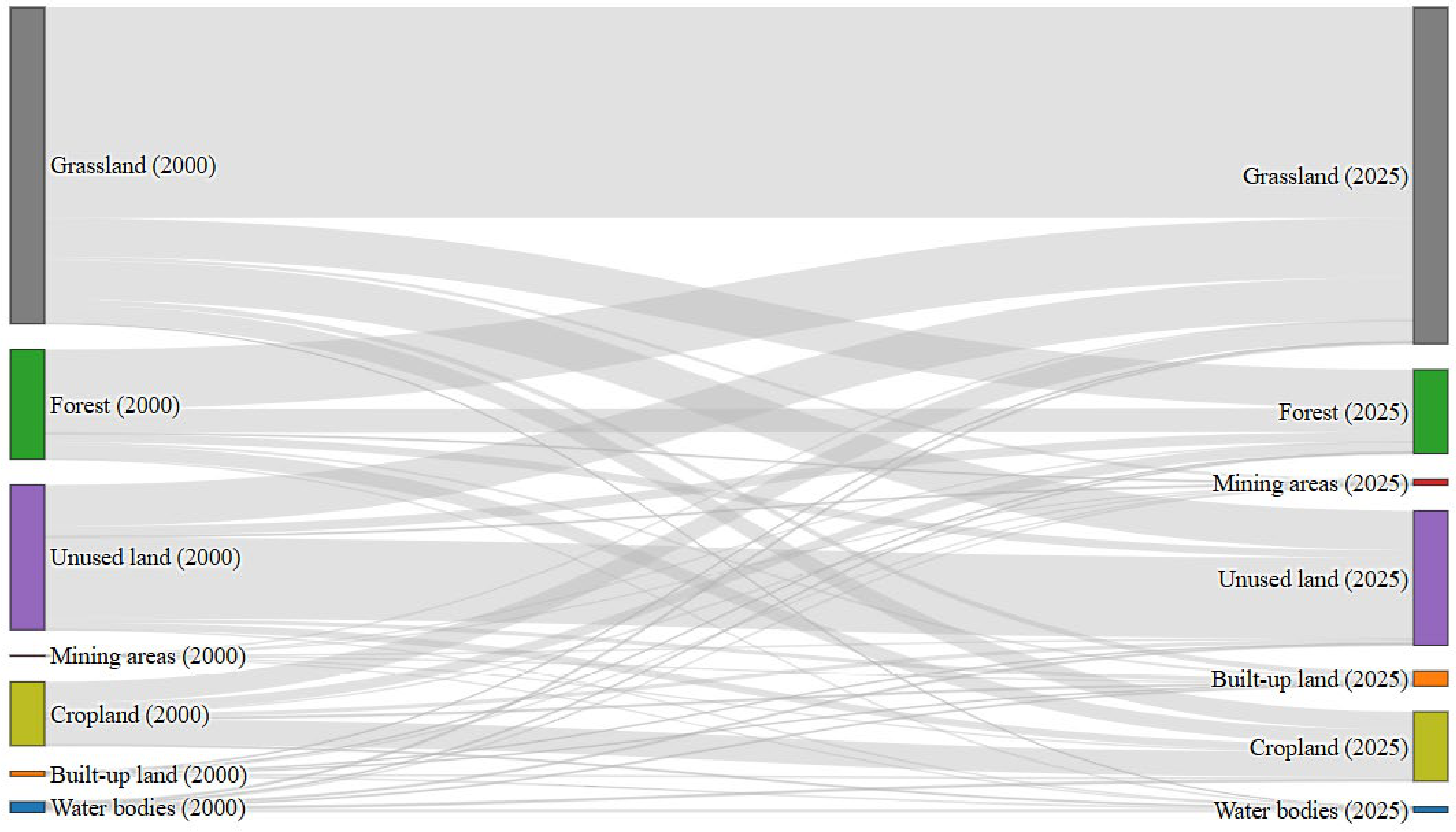
Figure 15 illustrates the Sankey diagram of land cover transitions in Ordos from 2000 to 2025, providing a visual representation of the dominant conversion pathways among different land cover classes. The results are consistent with those derived from the transition matrix analysis, further confirming that grassland and unused land serve as the primary sources of land cover transitions, while mining areas and built-up land exhibit continuous expansion over the study period.

4.4. Spatiotemporal Dynamics and Land-Cover-Based Ecological Quality Patterns

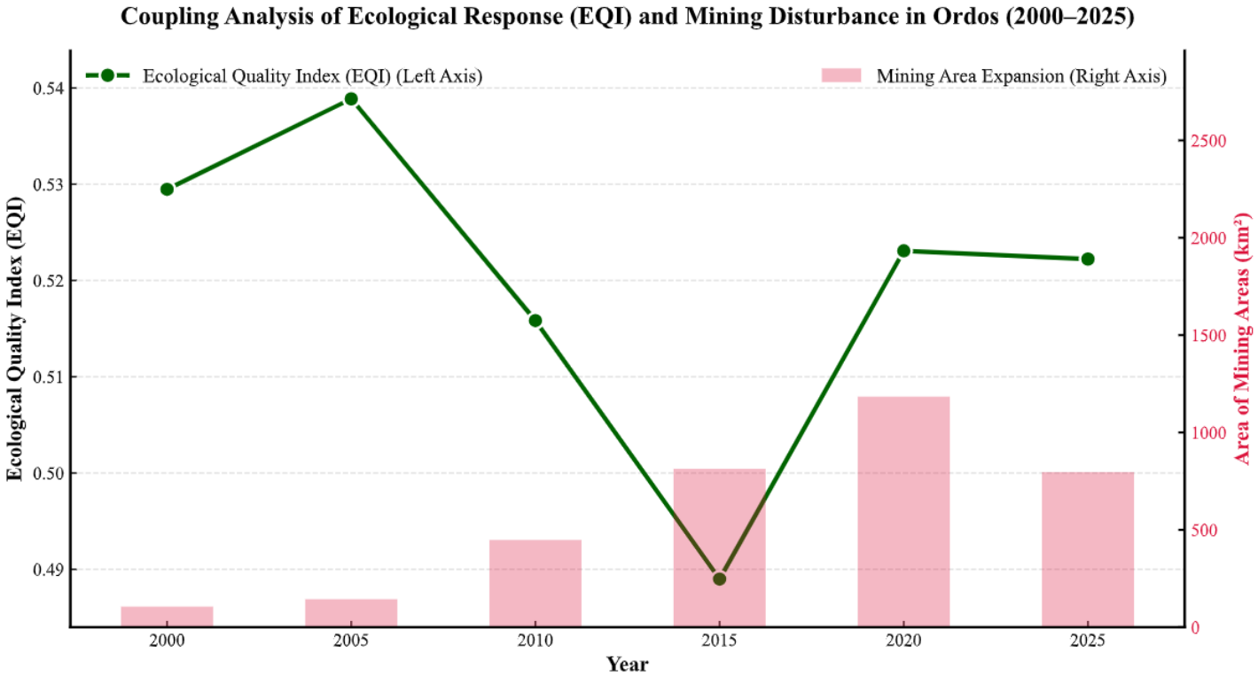
Based on the land-cover areas and ecological quality coefficients, the annual EQI values and class-level contributions were calculated, as shown in Table 14. The EQI decreased from 0.529 in 2000 to 0.489 in 2015 and then recovered to 0.522 in 2025. To provide a complementary vegetation-based perspective on vegetation change, MODIS growing-season mean NDVI was further compared with EQI (Table 15). NDVI increased from 0.186 in 2000 to 0.375 in 2025, with a slight decrease from 0.249 in 2010 to 0.241 in 2015. This pattern is partly consistent with the EQI trend, particularly the lower values around 2015 and the recovery after 2015. Differences between the two indicators are reasonable because EQI reflects land-cover composition and predefined ecological quality coefficients, whereas NDVI mainly represents vegetation greenness. The two indicators are therefore interpreted as providing complementary, rather than identical, information on environmental change. It should be noted that classification errors, particularly those involving classes with relatively low independent validation accuracy, such as forest, may propagate into the EQI estimates and introduce uncertainty into their ecological interpretation.
Figure 16 illustrates the spatiotemporal variation of the EQI derived from the ecological quality coefficients and the corresponding land-cover areas, together with mining disturbance patterns across the study period. In 2000, coal mining activities in Ordos were still at a relatively small scale and were mainly dominated by underground mining, which likely limited direct surface disturbance. During this period, ecological restoration initiatives such as the Grain for Green Program were being gradually implemented. The mining area was relatively small in 2000, which was consistent with the higher land-cover-based EQI observed during this period.
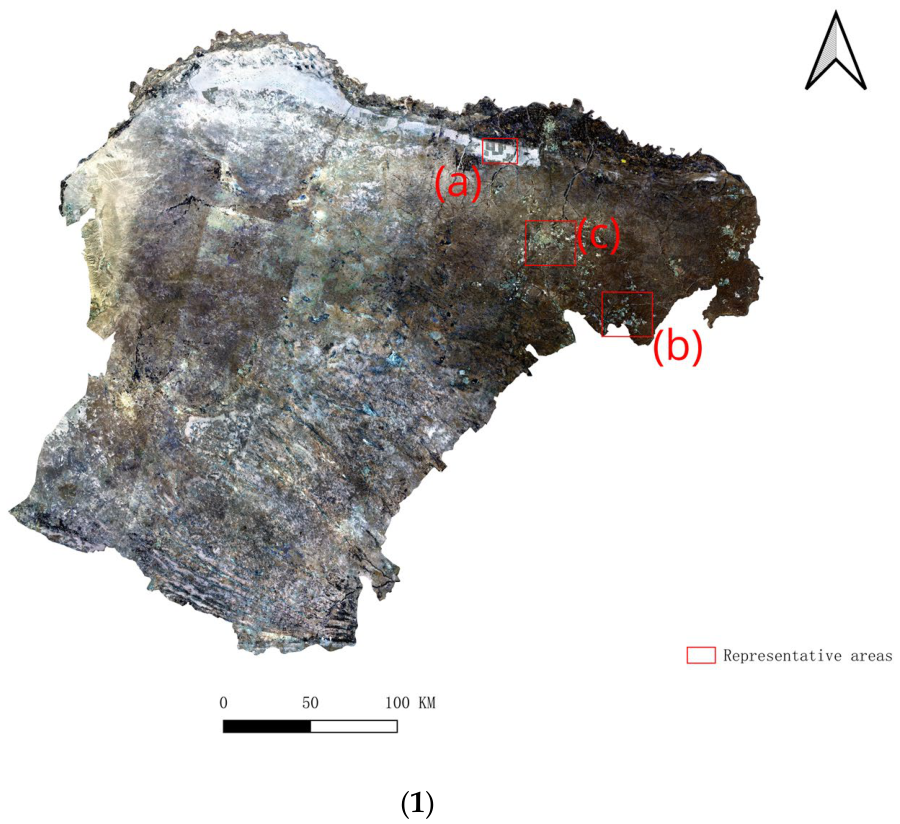
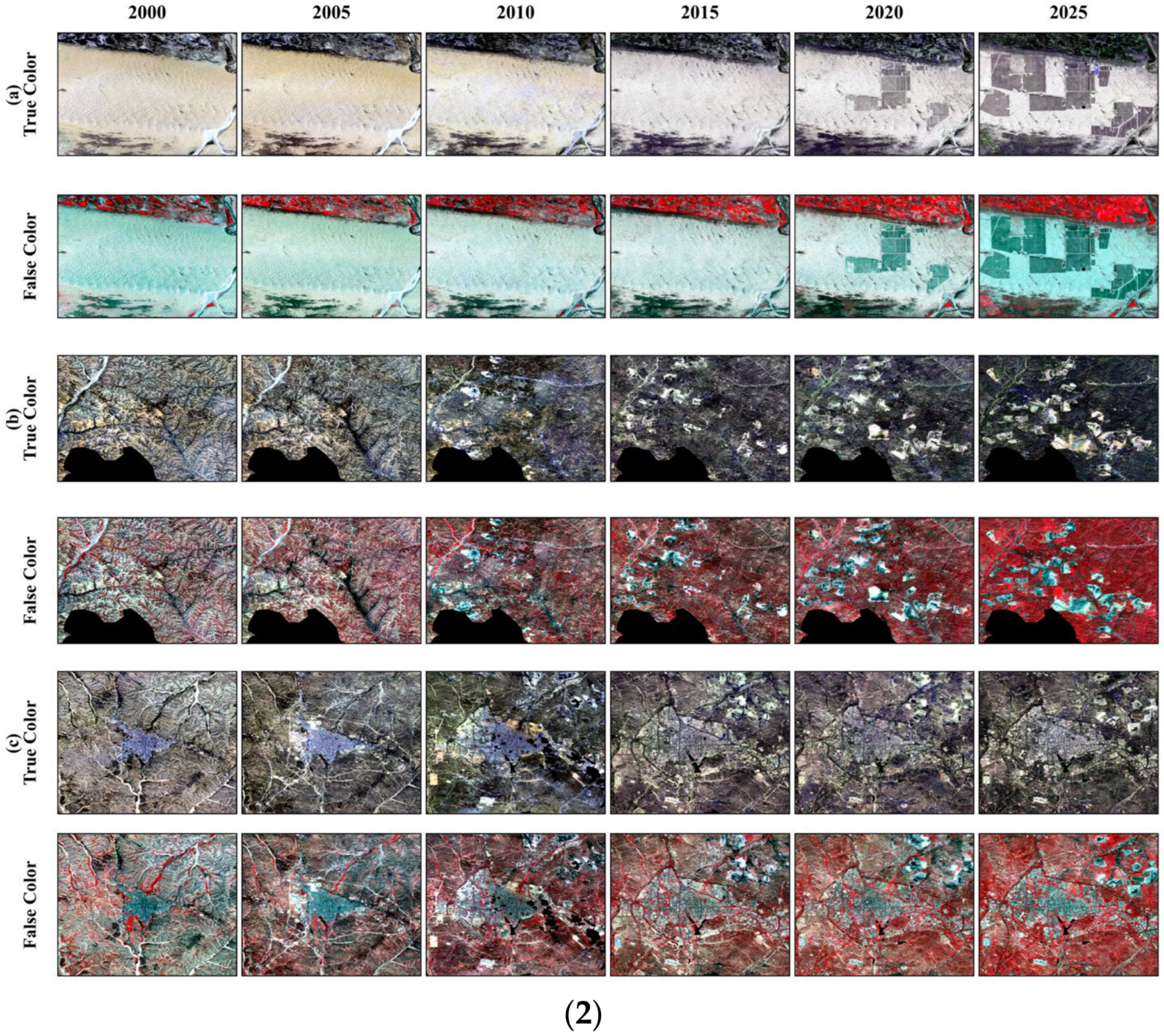
To provide spatial context for the representative areas shown in Figure 17, their approximate locations are identified in the left panel. Area (a) is approximately located in Dalad Banner (109.7757°E, 40.2547°N), area (b) in Jungar Banner (110.5518°E, 39.4300°N), and area (c) near the central urban area of Ordos (110.0344°E, 39.7965°N). These areas were selected as typical visual examples because they show clear land-cover transitions related to photovoltaic and infrastructure development, mining expansion, and reclamation or vegetation recovery, respectively. From 2005 to 2015, large-scale open-pit coal mining expanded under regional development strategies, and extensive grassland and surface vegetation were converted or disturbed during mining expansion (area (b) in Figure 17(2)). This period was associated with a noticeable decline in EQI. The spatial correspondence between mining expansion, vegetation disturbance, and EQI decline suggests that mining expansion was associated with the observed land-cover-based ecological quality pattern, although other factors such as climate variability, land management, and restoration policies may also have influenced the observed changes.
From 2015 to 2020, mining areas continued to expand while the land-cover-based EQI increased (area (c) in Figure 17(2)). This temporal pattern coincided with the implementation of ecological restoration activities alongside mining development. Reclamation of overburden dumps and vegetation restoration in mining areas were also observed during this period and may be associated with the upward land-cover-based EQI pattern.
From 2020 to 2025, the total area of mining areas decreased, while the land-cover-based EQI remained relatively stable. This period coincided with strengthened environmental regulation and the promotion of clean energy development, including large-scale photovoltaic deployment (area (a) in Figure 17(2)). Ecological restoration of abandoned mining areas also continued, with some reclaimed sites converted to grassland or repurposed for photovoltaic infrastructure. Together, these land-cover transitions were associated with a relatively stable ecological quality pattern during this period.
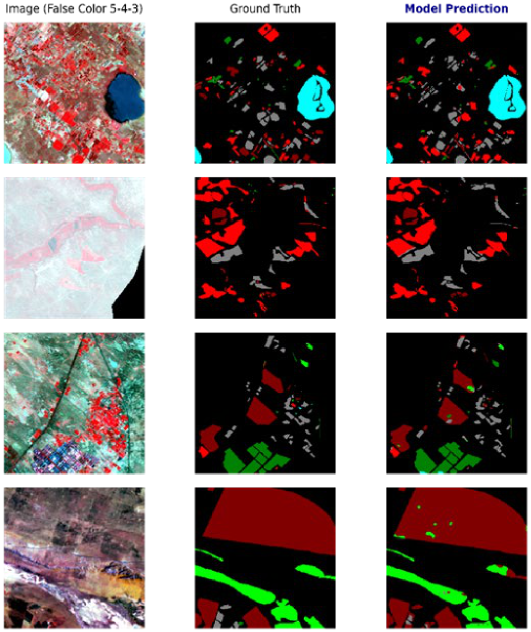
4.5. Spatiotemporal Variation of Ecological Contribution

The LEI of different land-cover transitions was calculated based on the ecological contribution formulation using spreadsheet-based computation. As shown in Table 16, from 2000 to 2025, positive LEI values were mainly associated with transitions from unused land to grassland, cropland to grassland, and unused land to forest. Among these, the transition from unused land to grassland showed the highest positive ecological contribution proportion (48.10%). Transitions from cropland to grassland (17.83%) and from unused land to forest (12.48%) also showed relatively high positive contributions to changes in the land-cover-based EQI. However, transitions from grassland to unused land accounted for a relatively high proportion of negative ecological contribution (41.22%), reflecting transitions between grassland and unused land in the study area. These patterns may be associated with mining activities, land degradation pressure, climate variability, and local land management changes.
Although mining areas and built-up land occupied relatively small proportions of the total area, transitions involving these land-cover types were associated with negative contributions to the land-cover-based EQI. Specifically, transitions from grassland to mining areas and built-up land reached 436.07 km2 and 733.10 km2, respectively. Forest-to-mining and forest-to-built-up transitions accounted for 129.43 km2 and 323.82 km2, respectively. These changes were mainly concentrated in resource-rich regions such as Dongsheng District, Jungar Banner, and Yijinhuoluo Banner, where intensive coal mining, energy exploitation, and urban expansion may have increased landscape fragmentation and environmental stress.
Overall, the total positive ecological contribution was slightly lower than the total negative ecological contribution, suggesting a mild overall decline in the land-cover-based EQI during 2000–2025. Transitions associated with grassland expansion and other restoration-related land-cover changes contributed positively to the land-cover-based EQI. These patterns indicate clear associations between land-cover transitions and ecological quality changes, although further evidence would be needed to fully identify the underlying processes. From a land-management perspective, the protection and restoration of grassland ecosystems remain important for future ecological management and land-use optimization in Ordos.

4.6. Chapter Summary

Overall, the land-cover-based EQI fluctuated over the study period, with similar values in 2000 and 2025. Remote sensing results indicate that, compared with 2000, the overall land-cover composition did not undergo abrupt structural change, suggesting that land development activities and ecological recovery processes coexisted at the regional scale. In addition, artificial vegetation and irrigated agricultural patterns observed along desert margins may reflect the influence of long-term land management and desertification control practices.
From a temporal perspective, 2000–2020 was characterized by intensive coal mining development, particularly in core resource-rich regions such as Dongsheng District and Jungar Banner, where mining expansion and built-up land growth were associated with pronounced landscape fragmentation and changes in land-cover composition. During 2020–2025, under the broader context of carbon neutrality targets and ecological protection strategies in the Yellow River Basin, parts of abandoned mining areas and degraded sandy lands were converted into photovoltaic installations, which is consistent with a transition toward low-carbon land-use transformation.
Changes in surface water extent were also observed during the study period. The reduction in water bodies may be associated with several factors, including mining-related dewatering, climate variability, and land management. Although some post-mining areas have evolved into stable or reclaimed water bodies, the overall water surface area showed a declining tendency during the study period. Nevertheless, given the fragile ecological background of the arid and semi-arid region, the ecosystem remains sensitive to disturbance, and long-term ecological stability still requires sustained restoration and management efforts.

5. Discussion

This study produced six land-cover maps for Ordos from 2000 to 2025, with mining areas treated as an independent class. This classification made it possible to quantify the expansion of mining areas and their conversions with grassland, unused land, forest, and cropland. A modified U-Net model incorporating an eight-channel input feature stack, group normalization, and OHEM was used to provide the classification basis for this analysis. The effectiveness of the proposed model was evaluated through baseline U-Net comparisons, ablation studies, and accuracy benchmarking against the ESA WorldCover product. Based on the derived land cover maps, land use transition matrices, EQI, and LEI were used to investigate spatiotemporal land-use dynamics and associated ecological quality patterns in Ordos from 2000 to 2025. In addition, MODIS growing-season mean NDVI was introduced as a complementary vegetation-based indicator for interpreting vegetation change alongside the land-cover-based EQI results. The results provide insights into land system evolution and land-cover-based ecological quality patterns and their associations with land-use change under intensive mining disturbance, offering implications for land use optimization, ecological restoration, and sustainable development in resource-based cities [5].
Although the proposed approach achieved strong performance in mining-area recognition, the results are still subject to limitations associated with model generalization capability, data availability, and spatiotemporal scale effects:
First, the proposed U-Net-based framework is effective for land use/land cover (LULC) classification in complex mining environments; however, its ability to explicitly model long-range spatial dependencies remains limited. This reflects a general constraint of convolution-based architectures in capturing global contextual information in high-resolution remote sensing imagery. With the rapid development of Transformer-based architecture and multi-scale feature learning strategies, future studies may explore their potential to further improve classification performance in heterogeneous mining areas.
Second, the study is based on multi-temporal Landsat imagery spanning 25 years. Despite the use of a consistent seasonal compositing window and spatial resolution, residual differences in spectral response between Landsat 5 and Landsat 8, together with interannual variations in acquisition conditions and surface states, may affect the temporal comparability of the land-cover maps, particularly around the sensor-transition period. This study did not apply additional cross-sensor radiometric normalization or calibration. Accordingly, unusual changes around the 2010–2015 sensor-transition interval should not be interpreted solely as actual land-cover transitions. Future studies could integrate higher-temporal-resolution datasets, in situ observations, and historical land-use records to further improve the robustness of long-term spatiotemporal analysis.
Third, the identification of mining areas in this study is primarily based on surface characteristics derived from optical remote sensing data. As a result, the analysis mainly captures open-pit mining activities, while underground mining operations and their associated surface disturbances cannot be effectively represented. Therefore, the observed mining dynamics primarily reflect surface disturbance patterns and do not capture the full range of mining-related land-cover changes.
Future research may further improve the comprehensive characterization of mining-related land use dynamics by integrating multi-source remote sensing data. Temporal consistency correction based on land-cover transition rules and adjacent-year land-cover trajectories could also be explored to reduce isolated and implausible changes in multi-temporal classification maps. In particular, the combination of InSAR-based deformation measurements, nighttime light observations, and mining activity datasets could enable more comprehensive identification and monitoring of different types of mining operations and their associated surface disturbances. In addition, extending the analysis to multiple representative coal resource-based cities would enable comparative analyses of land-use change under different resource exploitation regimes. Such cross-regional studies could identify both common patterns and regional differences. Advances in high-resolution remote sensing and intelligent interpretation methods may further improve the spatial detail, temporal coverage, and regional applicability of land-use monitoring, providing support for ecological protection and sustainable development in resource-based regions.

6. Conclusions

This study quantified the spatiotemporal dynamics of land-use change in Ordos over the past 25 years and examined associated land-cover-based ecological quality patterns. The main conclusions are as follows:
(1)
The modified U-Net framework achieved the highest IoU for mining areas among the compared models, reaching 69.61%, providing the classification basis for distinguishing mining areas from other spectrally confused land-cover types in the study area. The model incorporated multispectral and surface-temperature features, group normalization, and online hard example mining to improve feature discrimination under heterogeneous surface conditions in arid mining regions. It achieved an internal validation mIoU of 69.51%, mAcc of 81.65%, and pixel-level aAcc of 83.16%, supporting the reliability of the land-cover maps used for the subsequent land-use transition analysis.
(2)
From 2000 to 2025, grassland and unused land remained the dominant land-cover types. The area classified as mining increased from 105.83 km2 in 2000 to 1184.17 km2 in 2020, before declining to 796.20 km2 in 2025. These changes, together with the continued expansion of built-up land, highlight the role of mining and urban development in reshaping the regional land-use structure.
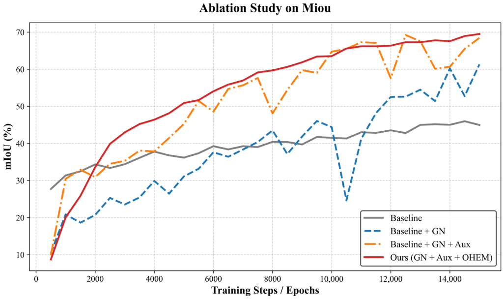
(3)
The land-cover-based EQI exhibited a decline-recovery–stabilization pattern. In the LEI results, transitions from unused land to grassland showed the largest positive contribution to changes in EQI, whereas transitions from grassland to unused land showed the largest negative contribution. These results identify the land-cover transitions most closely associated with the observed increases and decreases in land-cover-based EQI. This temporal pattern was consistent with the implementation of ecological restoration policies and land management measures, including grassland protection and mining regulation.
Overall, the mapped land-use transitions show substantial expansion and subsequent adjustment of mining areas, together with changes in grassland, unused land, and built-up land. These results provide a land-cover-based reference for grassland protection, mining-area reclamation, and land-use planning in Ordos. Future development should focus on balancing ecological conservation and resource utilization. Grassland ecosystems remain critical for maintaining regional ecological stability under arid and semi-arid conditions. Restoration of degraded grasslands and enhancement of ecosystem resilience are therefore important directions for long-term management. At the same time, controlling the spatial expansion of mining areas and built-up land is necessary to reduce landscape fragmentation. The mapped mining area increased from 105.83 km2 to 1184.17 km2 before declining to 796.20 km2. In mining-affected areas, land reclamation, vegetation restoration, and water resource protection remain key measures. From a technical perspective, remote sensing, GEE-based monitoring, and machine learning methods provide an effective framework for tracking land use dynamics. These approaches can support more continuous and detailed ecological monitoring in similar coal resource-based regions with intensive mining disturbance and arid or semi-arid environmental settings.

Author Contributions

Conceptualization, F.L. and P.L.; methodology, F.L. and J.C.; software, F.L.; validation, F.L. and J.C.; formal analysis, F.L.; investigation, H.X. and Q.G.; resources, P.L.; data curation, J.C. and Q.G.; writing—original draft preparation, F.L.; writing—review and editing, F.L., P.L. and J.C.; visualization, F.L. and J.C.; supervision, P.L.; project administration, P.L.; funding acquisition, P.L. software, J.X.; formal analysis, Y.M.; investigation, J.X., Y.W. and Y.M.; visualization, Y.W. and Y.M.; All authors have read and agreed to the published version of the manuscript.

Funding

This work was supported in part by the National Key Research and Development Program of China under Grant 2025ZD1011304, and the National Natural Science Foundation of China, grant number 52274169.

Data Availability Statement

The Landsat 5 TM and Landsat 8 OLI surface reflectance products used in this study were obtained from the United States Geological Survey (USGS) through the Google Earth Engine (GEE) platform. The manually labeled samples, model outputs, processed classification maps, and other derived datasets generated during this study are available from the corresponding author upon reasonable request.

Acknowledgments

The authors would like to thank the members of the research group for their valuable discussions and helpful suggestions during data processing, experimental analysis, and manuscript revision.

Conflicts of Interest

The authors declare no conflicts of interest.

References

  1. Turner, B.L.; Lambin, E.F.; Reenberg, A. The Emergence of Land Change Science for Global Environmental Change and Sustainability. Proc. Natl. Acad. Sci. USA 2007, 104, 20666–20671. [Google Scholar] [CrossRef] [Scilit] [PubMed]
  2. Foley, J.A.; DeFries, R.; Asner, G.P.; Barford, C.; Bonan, G.; Carpenter, S.R.; Chapin, F.S.; Coe, M.T.; Daily, G.C.; Gibbs, H.K.; et al. Global Consequences of Land Use. Science 2005, 309, 570–574. [Google Scholar] [CrossRef] [Scilit] [PubMed]
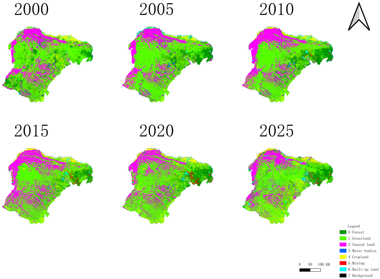
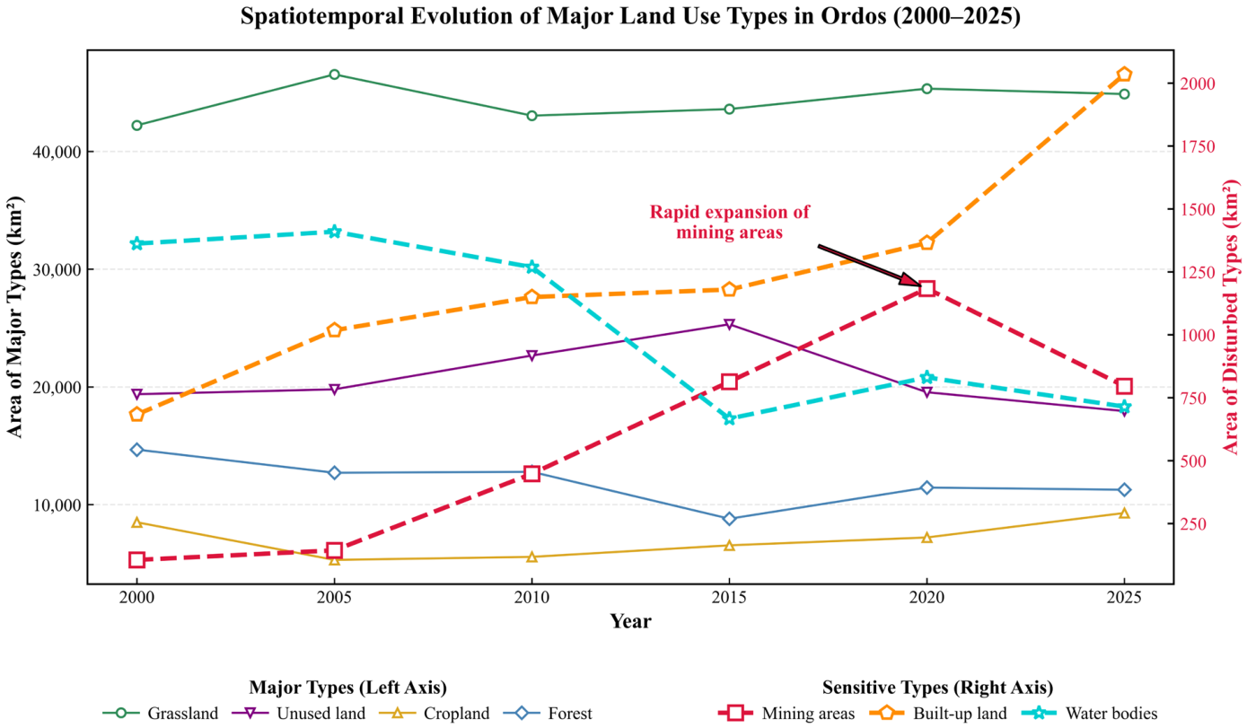
  3. Huang, J.; Yuan, X.; Lam, C.-T.; Wang, Y.; Xia, M. LCCDMamba: Visual State Space Model for Land Cover Change Detection of VHR Remote Sensing Images. IEEE J. Sel. Top. Appl. Earth Obs. Remote Sens. 2025, 18, 5765–5781. [Google Scholar] [CrossRef] [Scilit]
  4. Costanza, R.; d’Arge, R.; De Groot, R.; Farber, S.; Grasso, M.; Hannon, B.; Limburg, K.; Naeem, S.; O’Neill, R.V.; Paruelo, J.; et al. The Value of the World’s Ecosystem Services and Natural Capital. Nature 1997, 387, 253–260. [Google Scholar] [CrossRef] [Scilit]
  5. Alqadhi, S.; Bindajam, A.A.; Mallick, J.; Talukdar, S.; Rahman, A. Applying Deep Learning to Manage Urban Ecosystems in Arid Abha, Saudi Arabia: Remote Sensing-Based Modelling for Ecological Condition Assessment and Decision-Making. Heliyon 2024, 10, e25731. [Google Scholar] [CrossRef] [Scilit] [PubMed]
  6. State Council of the People’s Republic of China Notice of the State Council on Issuing the Sustainable Development Plan for National Resource-Based Cities (2013–2020). Available online: https://www.gov.cn/zwgk/2013-12/03/content_2540070.htm (accessed on 25 October 2025). (In Chinese)
  7. Tao, Y. Characteristics of Land Use Change and Construction of Ecological Security Pattern in Coal Resource-Based Cities. Ph.D. Dissertation, China University of Mining and Technology, Xuzhou, China, 2025. (In Chinese) [Google Scholar]
  8. Wen, B. Spatiotemporal Evolution and Simulation of Industrial and Mining Land in COAL resource-Exhausted Cities: A Case Study of Anyuan District, Pingxiang City, Jiangxi Province. Ph.D. Dissertation, Nanjing Agricultural University, Nanjing, China, 2024. (In Chinese) [Google Scholar]
  9. Townsend, P.A.; Helmers, D.P.; Kingdon, C.C.; McNeil, B.E.; De Beurs, K.M.; Eshleman, K.N. Changes in the Extent of Surface Mining and Reclamation in the Central Appalachians Detected Using a 1976–2006 Landsat Time Series. Remote Sens. Environ. 2009, 113, 62–72. [Google Scholar] [CrossRef] [Scilit]
  10. The People’s Government of Inner Mongolia Autonomous Region Ordos: Further Promoting High-Quality Development of the Coal Industry. Available online: https://www.nmg.gov.cn/ztzl/tjlswdrw/nyzlzyjd/202504/t20250407_2694121.html (accessed on 27 October 2025). (In Chinese)
  11. Bao, Y. An Analysis of Land-Use Change and Driving Force in Ordos. GSER 2024, 13, 240–252. [Google Scholar] [CrossRef]
  12. Zhang, Y.; Chen, Y. Analysis on the spatiotemporal evolution characteristics of ecosystem service value in Ordos City based on land use change. J. Arid Land Resour. Environ. 2025, 39, 131–140. (In Chinese) [Google Scholar] [CrossRef]
  13. Yan, G.; Zhang, Z. Dynamic changes and driving factors of land use in the Bojianghaizi watershed of the Ordos Plateau. Chin. J. Eco-Agric. 2017, 25, 1693–1706. (In Chinese) [Google Scholar] [CrossRef]
  14. Zanaga, D.; Van De Kerchove, R.; Daems, D.; De Keersmaecker, W.; Brockmann, C.; Kirches, G.; Wevers, J.; Cartus, O.; Santoro, M.; Fritz, S.; et al. ESA WorldCover 10 m 2021 V200. Zenodo 2022. [Google Scholar] [CrossRef]
  15. Hao, M.; Dong, X.; Jiang, D.; Yu, X.; Ding, F.; Zhuo, J. Land-Use Classification Based on High-Resolution Remote Sensing Imagery and Deep Learning Models. PLoS ONE 2024, 19, e0300473. [Google Scholar] [CrossRef] [Scilit] [PubMed]
  16. Oktay, O.; Schlemper, J.; Folgoc, L.L.; Lee, M.; Heinrich, M.; Misawa, K.; Mori, K.; McDonagh, S.; Hammerla, N.Y.; Kainz, B.; et al. Attention U-Net: Learning Where to Look for the Pancreas. arXiv 2018, arXiv:1804.03999. [Google Scholar]
  17. Wulder, M.A.; Masek, J.G.; Cohen, W.B.; Loveland, T.R.; Woodcock, C.E. Opening the Archive: How Free Data Has Enabled the Science and Monitoring Promise of Landsat. Remote Sens. Environ. 2012, 122, 2–10. [Google Scholar] [CrossRef] [Scilit]
  18. Hansen, M.C.; Potapov, P.V.; Moore, R.; Hancher, M.; Turubanova, S.A.; Tyukavina, A.; Thau, D.; Stehman, S.V.; Goetz, S.J.; Loveland, T.R.; et al. High-Resolution Global Maps of 21st-Century Forest Cover Change. Science 2013, 342, 850–853. [Google Scholar] [CrossRef] [Scilit] [PubMed]
  19. Zhu, Z.; Woodcock, C.E. Object-Based Cloud and Cloud Shadow Detection in Landsat Imagery. Remote Sens. Environ. 2012, 118, 83–94. [Google Scholar] [CrossRef] [Scilit]
  20. Zhu, Z.; Woodcock, C.E. Continuous Change Detection and Classification of Land Cover Using All Available Landsat Data. Remote Sens. Environ. 2014, 144, 152–171. [Google Scholar] [CrossRef] [Scilit]
  21. Gorelick, N.; Hancher, M.; Dixon, M.; Ilyushchenko, S.; Thau, D.; Moore, R. Google Earth Engine: Planetary-Scale Geospatial Analysis for Everyone. Remote Sens. Environ. 2017, 202, 18–27. [Google Scholar] [CrossRef] [Scilit]
  22. Breiman, L. Random Forests. Mach. Learn. 2001, 45, 5–32. [Google Scholar] [CrossRef] [Scilit]
  23. Ma, L.; Liu, Y.; Zhang, X.; Ye, Y.; Yin, G.; Johnson, B.A. Deep Learning in Remote Sensing Applications: A Meta-Analysis and Review. ISPRS J. Photogramm. Remote Sens. 2019, 152, 166–177. [Google Scholar] [CrossRef] [Scilit]
  24. Cortes, C.; Vapnik, V. Support-Vector Networks. Mach. Learn. 1995, 20, 273–297. [Google Scholar] [CrossRef] [Scilit]
  25. Congalton, R.G. A Review of Assessing the Accuracy of Classifications of Remotely Sensed Data. Remote Sens. Environ. 1991, 37, 35–46. [Google Scholar] [CrossRef] [Scilit]
  26. Foody, G.M. Status of Land Cover Classification Accuracy Assessment. Remote Sens. Environ. 2002, 80, 185–201. [Google Scholar] [CrossRef] [Scilit]
  27. Long, J.; Shelhamer, E.; Darrell, T. Fully Convolutional Networks for Semantic Segmentation. arXiv 2015, arXiv:1411.4038. [Google Scholar]
  28. Audebert, N.; Le Saux, B.; Lefèvre, S. Beyond RGB: Very High Resolution Urban Remote Sensing with Multimodal Deep Networks. ISPRS J. Photogramm. Remote Sens. 2018, 140, 20–32. [Google Scholar] [CrossRef] [Scilit]
  29. Volpi, M.; Tuia, D. Dense Semantic Labeling of Subdecimeter Resolution Images with Convolutional Neural Networks. IEEE Trans. Geosci. Remote Sens. 2017, 55, 881–893. [Google Scholar] [CrossRef] [Scilit]
  30. Marmanis, D.; Schindler, K.; Wegner, J.D.; Galliani, S.; Datcu, M.; Stilla, U. Classification with an Edge: Improving Semantic Image Segmentation with Boundary Detection. ISPRS J. Photogramm. Remote Sens. 2018, 135, 158–172. [Google Scholar] [CrossRef] [Scilit]
  31. Badrinarayanan, V.; Kendall, A.; Cipolla, R. SegNet: A Deep Convolutional Encoder-Decoder Architecture for Image Segmentation. IEEE Trans. Pattern Anal. Mach. Intell. 2017, 39, 2481–2495. [Google Scholar] [CrossRef] [Scilit] [PubMed]
  32. Ronneberger, O.; Fischer, P.; Brox, T. U-Net: Convolutional Networks for Biomedical Image Segmentation. arXiv 2015, arXiv:1505.04597. [Google Scholar]
  33. Zhou, Z.; Rahman Siddiquee, M.M.; Tajbakhsh, N.; Liang, J. UNet++: A Nested U-Net Architecture for Medical Image Segmentation. In Deep Learning in Medical Image Analysis and Multimodal Learning for Clinical Decision Support; Stoyanov, D., Taylor, Z., Carneiro, G., Syeda-Mahmood, T., Martel, A., Maier-Hein, L., Tavares, J.M.R.S., Bradley, A., Papa, J.P., Belagiannis, V., et al., Eds.; Lecture Notes in Computer Science; Springer International Publishing: Cham, Switzerland, 2018; Volume 11045, pp. 3–11. ISBN 978-3-030-00888-8. [Google Scholar]
  34. Diakogiannis, F.I.; Waldner, F.; Caccetta, P.; Wu, C. ResUNet-a: A Deep Learning Framework for Semantic Segmentation of Remotely Sensed Data. ISPRS J. Photogramm. Remote Sens. 2020, 162, 94–114. [Google Scholar] [CrossRef] [Scilit]
  35. He, K.; Zhang, X.; Ren, S.; Sun, J. Deep Residual Learning for Image Recognition. In Proceedings of the 2016 IEEE Conference on Computer Vision and Pattern Recognition (CVPR); IEEE: Las Vegas, NV, USA, 2016; pp. 770–778. [Google Scholar]
  36. Chen, L.-C.; Zhu, Y.; Papandreou, G.; Schroff, F.; Adam, H. Encoder-Decoder with Atrous Separable Convolution for Semantic Image Segmentation. In Computer Vision—ECCV 2018; Ferrari, V., Hebert, M., Sminchisescu, C., Weiss, Y., Eds.; Lecture Notes in Computer Science; Springer International Publishing: Cham, Switzerland, 2018; Volume 11211, pp. 833–851. ISBN 978-3-030-01233-5. [Google Scholar]
  37. Dosovitskiy, A.; Beyer, L.; Kolesnikov, A.; Weissenborn, D.; Zhai, X.; Unterthiner, T.; Dehghani, M.; Minderer, M.; Heigold, G.; Gelly, S.; et al. An Image Is Worth 16x16 Words: Transformers for Image Recognition at Scale. arXiv 2020, arXiv:2010.11929. [Google Scholar]
  38. Vaghela, R.; Vaishnani, D.; Srinivasu, P.N.; Popat, Y.; Sarda, J.; Woźniak, M.; Ijaz, M.F. Land Cover Classification for Identifying the Agriculture Fields Using Versions of YOLO V8. IEEE J. Sel. Top. Appl. Earth Obs. Remote Sens. 2025, 18, 8672–8684. [Google Scholar] [CrossRef] [Scilit]
  39. Rubab, S.; Khan, M.A.; Hamza, A.; Albarakati, H.M.; Saidani, O.; Alshardan, A.; Alasiry, A.; Marzougui, M.; Nam, Y. A Novel Network-Level Fusion Architecture of Proposed Self-Attention and Vision Transformer Models for Land Use and Land Cover Classification From Remote Sensing Images. IEEE J. Sel. Top. Appl. Earth Obs. Remote Sens. 2024, 17, 13135–13148. [Google Scholar] [CrossRef] [Scilit]
  40. Liu, Z.; Lin, Y.; Cao, Y.; Hu, H.; Wei, Y.; Zhang, Z.; Lin, S.; Guo, B. Swin Transformer: Hierarchical Vision Transformer Using Shifted Windows. In Proceedings of the 2021 IEEE/CVF International Conference on Computer Vision (ICCV); IEEE: Montreal, QC, Canada, 2021; pp. 9992–10002. [Google Scholar]
  41. Xie, E.; Wang, W.; Yu, Z.; Anandkumar, A.; Alvarez, J.M.; Luo, P. SegFormer: Simple and Efficient Design for Semantic Segmentation with Transformers. arXiv 2021, arXiv:2105.15203. [Google Scholar]
  42. Pan, J.; Chen, T.; Jia, K.; Plaza, A. Toward Sustainable Mining Landscapes: Evaluating Spatiotemporal Changes and Driving Mechanisms of Eco-Environmental Quality in Central China. IEEE J. Sel. Top. Appl. Earth Obs. Remote Sens. 2025, 18, 21144–21155. [Google Scholar] [CrossRef] [Scilit]
  43. Zhao, H.; Shi, J.; Qi, X.; Wang, X.; Jia, J. Pyramid Scene Parsing Network. In Proceedings of the 2017 IEEE Conference on Computer Vision and Pattern Recognition (CVPR); IEEE: Honolulu, HI, USA, 2017; pp. 6230–6239. [Google Scholar]
  44. Zhang, Z.; Liu, Q.; Wang, Y. Road Extraction by Deep Residual U-Net. IEEE Geosci. Remote Sens. Lett. 2018, 15, 749–753. [Google Scholar] [CrossRef] [Scilit]
  45. Rakhlin, A.; Davydow, A.; Nikolenko, S. Land Cover Classification from Satellite Imagery with U-Net and Lovász-Softmax Loss. In Proceedings of the 2018 IEEE/CVF Conference on Computer Vision and Pattern Recognition Workshops (CVPRW); IEEE: Salt Lake City, UT, USA, 2018; pp. 257–2574. [Google Scholar]
  46. Xiao, D.; Yin, L.; Fu, Y. Open-Pit Mine Road Extraction from High-Resolution Remote Sensing Images Using RATT-UNet. IEEE Geosci. Remote Sens. Lett. 2022, 19, 3002205. [Google Scholar] [CrossRef] [Scilit]
  47. Xie, G. Improvement of the Valuation Method for Ecosystem Services Based on Standard Equivalent Factor Value per Unit Area. J. Nat. Resour. 2015, 30, 1243. (In Chinese) [Google Scholar] [CrossRef]
  48. Xu, H. A Remote Sensing Urban Ecological Index and Its Application. Shengtai Xuebao/Acta Ecol. Sin. 2013, 33, 7853–7862. [Google Scholar]
  49. Xu, H. A remote sensing index for assessment of regional ecological changes. China Environ. Sci. 2013, 33, 889–897. (In Chinese) [Google Scholar] [CrossRef]
  50. Olofsson, P.; Foody, G.M.; Herold, M.; Stehman, S.V.; Woodcock, C.E.; Wulder, M.A. Good Practices for Estimating Area and Assessing Accuracy of Land Change. Remote Sens. Environ. 2014, 148, 42–57. [Google Scholar] [CrossRef] [Scilit]
  51. You, C.; Jiao, L.; Liu, X.; Li, L.; Liu, F.; Ma, W.; Yang, S. Boundary-Aware Multiscale Learning Perception for Remote Sensing Image Segmentation. IEEE Trans. Geosci. Remote Sens. 2023, 61, 4407115. [Google Scholar] [CrossRef] [Scilit]
  52. Jonnala, N.S.; Bheemana, R.C.; Prakash, K.; Bansal, S.; Jain, A.; Pandey, V.; Faruque, M.R.I.; Al-mugren, K.S. DSIA U-Net: Deep Shallow Interaction with Attention Mechanism UNet for Remote Sensing Satellite Images. Sci. Rep. 2025, 15, 549. [Google Scholar] [CrossRef] [Scilit] [PubMed]
  53. Wu, Y.; He, K. Group Normalization. In Proceedings of the European Conference on Computer Vision (ECCV); Springer: Berlin/Heidelberg, Germany, 2018; pp. 3–19. [Google Scholar]
  54. Bengio, Y.; Simard, P.; Frasconi, P. Learning Long-Term Dependencies with Gradient Descent Is Difficult. IEEE Trans. Neural Netw. 1994, 5, 157–166. [Google Scholar] [CrossRef] [Scilit] [PubMed]
  55. Lee, C.-Y.; Xie, S.; Gallagher, P.; Zhang, Z.; Tu, Z. Deeply-Supervised Nets. Available online: https://arxiv.org/abs/1409.5185v2 (accessed on 2 July 2026).
  56. Shrivastava, A.; Gupta, A.; Girshick, R. Training Region-Based Object Detectors with Online Hard Example Mining. arXiv 2016, arXiv:1604.03540. [Google Scholar]
  57. Panuntun, I.A.; Chen, Y.-N.; Jamaluddin, I.; Tran, T.L.C. Evaluation of Deep Learning Semantic Segmentation for Land Cover Mapping on Multispectral, Hyperspectral and High Spatial Aerial Imagery. arXiv 2024, arXiv:2406.14220. [Google Scholar]
  58. Luo, M.; Ji, S. Cross-Spatiotemporal Land-Cover Classification from VHR Remote Sensing Images with Deep Learning Based Domain Adaptation. ISPRS J. Photogramm. Remote Sens. 2022, 191, 105–128. [Google Scholar] [CrossRef] [Scilit]
Figure 1. Location map of the study area.
Remotesensing 18 03131 g001
Figure 2. Spatial distribution of land use classification samples in Ordos City. Colored areas indicate manually annotated samples of different land-cover classes.
Remotesensing 18 03131 g002
Figure 3. Image patches and their corresponding ground truth labels.
Remotesensing 18 03131 g003
Figure 4. Overall research workflow.
Remotesensing 18 03131 g004
Figure 5. Architecture of the Improved U-Net.
Remotesensing 18 03131 g005
Figure 6. Architectural comparison between BN and GN.
Remotesensing 18 03131 g006
Figure 7. Structure of the deep supervision mechanism.
Remotesensing 18 03131 g007
Figure 8. Schematic diagram of the OHEM mechanism.
Remotesensing 18 03131 g008
Figure 9. Training dynamic curves of the improved U-Net model. (a) Training loss convergence curve; (b) validation mIoU upward curve.
Remotesensing 18 03131 g009
Figure 10. Qualitative Classification Results of the Proposed U-Net Model on the Validation Set.
Remotesensing 18 03131 g010
Figure 11. Comparison of validation mIoU curves for different ablation configurations.
Remotesensing 18 03131 g011
Figure 12. Comparison of training loss curves for different ablation configurations.
Remotesensing 18 03131 g012
Figure 13. Multi-temporal land cover classification results of Ordos.
Remotesensing 18 03131 g013
Figure 14. Spatiotemporal evolution of major land cover classes in Ordos from 2000 to 2025.
Remotesensing 18 03131 g014
Figure 15. Dynamic land use transition flows between 2000 and 2025.
Remotesensing 18 03131 g015
Figure 16. Ecological Quality and Mining Disturbance in Ordos (2000–2025).
Remotesensing 18 03131 g016
Figure 17. Locations and multi-temporal Landsat image patches of the representative areas in Ordos. (1) shows the locations of the representative areas within Ordos City, where area (a) is approximately located in Dalad Banner, area (b) in Jungar Banner, and area (c) in the central urban area of Ordos. The red rectangles indicate the approximate spatial extents of the representative areas. (2) shows the corresponding multi-temporal Landsat image patches from 2000 to 2025, including true-color and false-color composites.
Remotesensing 18 03131 g017aRemotesensing 18 03131 g017b
Table 1. Comparison between representative studies and this study.
StudyStudy Area/ObjectSelf-Classified Land Use?Mining Area as an Independent Class?Long Time Series?Deep Learning Used?Linked with Ecological Assessment?
Townsend et al. [9]Surface mining and reclamation in Central AppalachiansYesYesYes, 1976–2006NoPartly
Bao [11]Land-use change in OrdosYes/PartlyNoPartlyNoNo/Partly
Zhang et al. [12]Land-use change and ecosystem service value in OrdosNo/PartlyNoYes, 2000–2020NoYes
Pan et al. [42]Eco-environmental quality in a mining area of Central ChinaNoNoYes/PartlyNoYes
Hao et al. [15]Land-use classification using high-resolution remote sensing imageryYesNoNoYesNo
This studyOrdos, a typical coal resource-based city in ChinaYesYesYes, 2000–2025YesYes
Note: The contribution of this study lies in examining the land-use implications of mapping mining areas as a separate class; the classification, transition analysis, and ecological assessment components are used to support this research question.
Table 2. Landsat image sources and annual compositing strategy used in this study.
YearCompositing MethodSpatial
Resolution
SensorGEE Image CollectionAcquisition WindowCloud ControlCloud/Shadow Masking
2000Cloud-masked median composite30 mLandsat 5 TMLANDSAT/LT05/C02/T1_L2June 1–September 30Scene-level cloud-cover filteringQA_PIXEL cloud and cloud-shadow bits
200530 mLandsat 5 TMLANDSAT/LT05/C02/T1_L2
201030 mLandsat 5 TMLANDSAT/LT05/C02/T1_L2
201530 mLandsat 8 OLI/TIRSLANDSAT/LC08/C02/T1_L2
202030 mLandsat 8 OLI/TIRSLANDSAT/LC08/C02/T1_L2
202530 mLandsat 8 OLI/TIRSLANDSAT/LC08/C02/T1_L2
Note: For each target year, all eligible scenes covering Ordos within the acquisition window were processed in GEE. Cloud and cloud-shadow pixels were masked using the QA_PIXEL band, and a median reducer was applied to generate an annual cloud-reduced mosaic.
Table 3. Ecological quality coefficients of land-use types.
No.Land-Use TypeEcological Environmental Quality Index
1Cropland0.27
2Forest land0.76
3Grassland0.70
4Water body0.54
5Built-up land0.20
6Mining areas0.18
7Unused land0.11
Note: The EQI coefficients are consistent with commonly used land-use ecological value classification schemes reported in previous studies and are used here as dimensionless relative weights for comparative analysis within the study area, rather than for absolute ecological valuation.
Table 4. Construction of the eight-channel input feature stack for Landsat 8 and Landsat 5.
Unified Input ChannelLandsat 8 OLI/TIRS BandLandsat 5 TM Band
B1SR_B1SR_B1
B2SR_B2SR_B1
B3SR_B3SR_B2
B4SR_B4SR_B3
B5SR_B5SR_B4
B6SR_B6SR_B5
B7SR_B7SR_B7
B8ST_B10ST_B6
Note: Landsat 5 SR_B1 was duplicated in the first two input channels to maintain an eight-channel input because Landsat 5 lacks a coastal aerosol band corresponding to Landsat 8 SR_B1.
Table 5. Accuracy Assessment for Individual Land Cover Classes.
ClassIoUClass Acc
Cropland89.2092.48
Grassland80.2891.22
Unused land65.7778.85
Water bodies62.5175.94
Built-up land60.8871.56
Forest58.3272.81
Mining69.6188.72
mIoU69.51-
mAcc-81.65
aAcc-83.16
Note: IoU denotes Intersection over Union; Class Acc denotes class accuracy, calculated as the ratio of correctly classified pixels to all reference pixels for a given class. mIoU and mAcc denote the mean IoU and mean class accuracy across all classes, respectively; aAcc denotes pixel-level overall accuracy. All values are expressed in percentage (%).
Table 6. Overall ablation results of different model configurations.
Model ConfigurationBest IteraAcc (%)mAcc (%)mIoU (%)
U-Net14,50075.3959.9145.99
U-Net + GN15,00078.6673.8361.33
U-Net + GN + Auxiliary supervision12,50080.8580.7069.25
U-Net + GN + Auxiliary supervision + OHEM15,00083.1681.6569.51
Table 7. Class-level IoU ablation results of different model configurations.
Model ConfigurationCroplandGrasslandUnused LandWater BodiesBuilt-Up LandMining AreasForest
U-Net85.240.0065.130.0065.7556.6849.13
U-Net + GN82.7755.8464.6058.5463.4258.9045.27
U-Net + GN + Auxiliary supervision76.3182.0459.7377.7959.9664.0264.88
U-Net + GN + Auxiliary supervision + OHEM89.2080.2865.7762.5160.8869.6158.32
Note: Values in this table represent IoU (%) for each land-cover class.
Table 8. Accuracy comparison of different segmentation models for land-use classification.
ModelaAcc (%)mAcc (%)mIoU (%)Mining IoU (%)
U-Net75.3959.9145.9956.68
ResUNet75.3171.8959.4249.12
DeepLabV3+ (ResNet-18)82.2282.9468.5867.04
FCN (ResNet-18)83.9984.8972.5368.05
PSPNet (ResNet-18)84.6184.9273.1668.32
SegNet84.7984.1975.1164.76
Our83.1681.6569.5169.61
Table 9. Robustness analysis of the proposed model under different random seeds.
RunSeedaAcc (%)mAcc (%)mIoU (%)Mining IoU (%)
Final model used in this studyOriginal run83.1681.6569.5169.61
Repeated run082.7181.0169.2069.34
Repeated run4282.8381.1268.8669.37
Repeated run202582.6880.9568.8468.28
Mean ± SD of repeated runs0/42/202582.74 ± 0.0881.03 ± 0.0968.97 ± 0.2069.00 ± 0.62
Table 10. Computational complexity comparison of different model configurations.
ModelGFLOPsParams (M)mIoU (%)Mining IoU (%)
U-Net49.1128.9645.9956.68
U-Net + GN49.2328.9661.3358.90
U-Net + GN + Auxiliary supervision49.2328.9669.2564.02
ResUNet60.4033.1459.4249.12
Our49.2328.9669.5169.61
Table 11. Comparison of Classification Accuracy Between the Proposed U-Net Model and the ESA WorldCover.
ClassPA (%)UA (%)F1 (%)ESA-F1(%)
Unused land93.075.083.054.5
Water bodies70.093.380.086.7
Cropland70.085.476.977.5
Mining areas60.080.068.60.0
Forest37.045.140.70.0
Built-up land46.071.956.143.3
Grassland86.043.457.737.5
OA66.048.7
Kappa0.6030.402
Note: PA, Producer’s Accuracy; UA, User’s Accuracy; F1, F1-score; ESA-F1, F1-score of the ESA WorldCover product.
Table 12. Statistics of Land Cover Areas in Ordos From 2000 to 2025.
Years200020052010201520202025
Classes
Forest (km2)14,674.5412,709.2412,788.098802.6011,449.2311,266.35
Grassland (km2)42,222.5546,548.7743,044.7143,603.7045,338.4244,880.41
Unused land (km2)19,380.0819,795.9822,666.9925,319.3019,549.4117,947.55
Water bodies (km2)1362.431409.731268.89666.97830.95714.62
Cropland (km2)8501.475304.645562.266542.017211.509291.28
Mining areas (km2)105.83143.74448.03813.751184.17796.20
Built-up land (km2)683.501018.121150.221179.761365.272034.64
Total area (km2)86,930.3986,930.2486,929.1986,928.0986,928.9686,931.04
Table 13. Land Cover Transition Matrix (2000–2025).
2025ForestGrasslandUnused LandWater BodiesCroplandMiningBuilt-Up Land
2000
Forest3184.54837984.13221100.610922.83391929.1599129.4272323.8227
Grassland5168.707228,136.52275216.825761.38362469.9294436.0716733.1049
Unused land1312.85885574.667510,766.932223.7357999.4671144.8694557.55
Water bodies129.942215.6418194.3523409.2237228.726946.1961138.348
Cropland1367.79752835.9243545.6574146.11233382.583433.6816189.7119
Mining areas13.624238.300429.09341.444514.83381.37797.1532
Note: Values represent transition areas (km2) between land cover classes derived from the classification results.
Table 14. Ecological Quality of Land Cover Classes Across Years.
YearsForestGrasslandWater BodiesCroplandMiningBuilt-Up LandUnused LandEQI
20000.1282940.3399940.0084630.0264050.0002190.0015730.0245230.529471
20050.1111120.3748310.0087570.0164760.0002980.0023420.0250490.538866
20100.1118030.3466190.0078820.0172760.0009280.0026460.0286830.515837
20150.076960.3511250.0041430.020320.0016850.0027140.0320390.488986
20200.1000980.365090.0051620.0223990.0024520.0031410.0247380.52308
20250.0984970.3613930.0044390.0288580.0016490.0046810.022710.522227
Table 15. Annual EQI and MODIS NDVI.
YearsEQIMODIS Mean NDVI
20000.5294710.185618843
20050.5388660.215445961
20100.5158370.249439229
20150.4889860.241481531
20200.523080.287942423
20250.5222270.375083244
Note: MODIS NDVI represents the growing-season mean value from June 1 to September 30.
Table 16. Land Cover Transition Types, Transition Areas, and Ecological Contribution (LEI) from 2000 to 2025.
2000–2025Land Cover TransitionTransition Area (km2)LEIContribution (%)
Improving transitionsUnused land → Grassland5574.66750.03783648.1008
Cropland → Grassland2835.92430.01402817.8338
Unused land → Forest1312.85880.00981712.48
Cropland → Forest1367.79750.007719.8017
Grassland → Forest5168.70720.0035684.5354
Unused land → Cropland999.46710.001842.3387
Unused land → Built-up land557.550.0005770.7339
Built-up land → Forest88.71930.0005720.7266
Built-up land → Grassland95.12370.0005470.6956
Cropland → Water bodies146.11230.0004540.5769
Water bodies → Grassland215.64180.0003970.5046
Water bodies → Forest129.9420.0003290.4181
Mining areas → Grassland38.30040.0002290.2913
Built-up land → Cropland266.40810.0002150.2727
Built-up land → Water bodies49.81410.0001950.2477
Mining areas → Forest13.62420.0000910.1152
Mining areas → Cropland14.83380.0000150.0186
Mining areas → Built-up land7.15320.0000020.0227
Total LEI 0.078659
Degrading transitionsGrassland → Unused land5216.82570.03540741.2177
Grassland → Cropland2469.92940.01221814.2226
Forest → Cropland1929.15990.01087412.6587
Forest → Unused land1100.61090.008239.5802
Forest → Grassland7984.13220.0055116.4151
Grassland → Built-up land733.10490.0042174.9086
Grassland → Mining areas436.07160.0026093.0366
Forest → Built-up land323.82270.0020862.4284
Cropland → Unused land545.65740.0010041.1691
Water bodies → Unused land194.35230.0009611.1191
Forest → Mining areas129.42720.0008641.0053
Water bodies → Cropland228.72690.000710.827
Water bodies → Built-up land138.3480.0005410.6299
Water bodies → Mining areas46.19610.0001910.2227
Cropland → Built-up land189.71190.0001530.1778
Cropland → Mining areas33.68160.0000350.0409
Built-up land → Mining areas4.56390.0000010.0011
Total LEI 0.085903
Disclaimer/Publisher’s Note: The statements, opinions and data contained in all publications are solely those of the individual author(s) and contributor(s) and not of MDPI and/or the editor(s). MDPI and/or the editor(s) disclaim responsibility for any injury to people or property resulting from any ideas, methods, instructions or products referred to in the content.