Evidence-Based Reliability Assessment of Spatial Transfer Learning for Satellite-Derived Ground Deformation Monitoring

Highlights

What are the main findings?

• A transferability-aware framework was developed to predict satellite-derived ground deformation by combining local observations with knowledge transferred from environmentally similar monitoring tasks.
• An evidence-based reliability framework accompanies every prediction with independent evidence reliability, transfer reliability, and validation-calibrated expected prediction error, extending transfer learning beyond prediction accuracy.

What are the implications of the main findings?

• Within the investigated study area, environmental similarity emerged as a stronger indicator of successful spatial knowledge transfer than structural similarity, supporting more reliable source-task selection.
• Deployment-oriented reliability profiles enable infrastructure managers to prioritise monitoring and maintenance by jointly considering deformation hazard, confidence in available evidence, and expected prediction uncertainty.

Abstract

Satellite-derived ground deformation monitoring has become an essential tool for infrastructure management; however, the spatial heterogeneity of Interferometric Synthetic Aperture Radar (InSAR) observations limits reliable assessment in regions with sparse measurement coverage. While spatial transfer learning offers a practical means of extending deformation predictions beyond well-observed areas, existing approaches primarily emphasise predictive accuracy and provide little indication of whether transferred predictions can be trusted during operational deployment. This study presents an evidence-based reliability assessment framework for spatial transfer learning using European Ground Motion Service (EGMS) observations. The framework accompanies every prediction with complementary evidence reliability, transfer reliability, and validation-calibrated expected prediction error. The methodology was evaluated within a single 100 km × 100 km EGMS tile in Eastern England, characterised by gradual, subsidence-type ground motion, using 815 EGMS observations and deployed to assess deformation risk for 140 road corridors. The proposed local–transfer fusion achieved a mean RMSE of 1.720 mm yr⁻¹, outperforming multi-source transfer strategies. Feature–space divergence exhibited a significant positive relationship with transfer prediction error ($\rho =0.515$, $p<0.001$), demonstrating that environmental similarity is a stronger indicator of transfer success than structural similarity within the investigated study area. The proposed framework extends conventional transfer learning beyond prediction accuracy and provides a practical foundation for risk-informed infrastructure monitoring using satellite-derived ground deformation observations.

1. Introduction

Ground deformation is one of the most significant geohazards affecting the long-term performance and safety of civil infrastructure. Processes such as land subsidence, groundwater abstraction, mining activities, slope instability, and soil consolidation can progressively damage roads, railways, pipelines, and buildings, resulting in increased maintenance costs and elevated safety risks. Continuous monitoring of ground deformation is therefore fundamental to infrastructure asset management, hazard mitigation, and sustainable urban development [1,2,3,4]. The increasing availability of Earth observation data has substantially improved the ability to monitor these processes over large geographical regions, enabling more comprehensive assessments than are achievable using conventional ground-based surveying alone [5,6].

Although satellite-derived deformation products provide extensive spatial coverage, observational support remains inherently heterogeneous. Measurement availability depends on factors such as land cover, radar coherence, acquisition geometry, and revisit frequency, resulting in dense observations in some regions and sparse measurements in others [7,8]. Consequently, many infrastructure corridors continue to lack sufficient observations for reliable deformation assessment, creating a need for predictive approaches capable of extending deformation information beyond directly observed locations.

Machine learning has emerged as an effective means of exploiting environmental and geospatial information to predict deformation patterns where observations are limited. Recent studies have demonstrated the capability of tree-based ensembles, neural networks, and other data-driven approaches for subsidence prediction, deformation forecasting, and geotechnical risk assessment [9,10,11,12,13]. However, most predictive models are developed using observations collected within a single geographical region, limiting their applicability in operational settings where labelled deformation measurements are sparse or unavailable.

Transfer learning offers a promising alternative by enabling knowledge acquired from data-rich regions to support prediction in related but data-poor environments [14,15,16]. Nevertheless, successful transfer cannot be assumed solely from predictive accuracy. The effectiveness of transferred knowledge depends on the compatibility between source and target regions, while inappropriate transfer may introduce negative transfer and reduce prediction quality [17]. At the same time, recent advances in uncertainty quantification have highlighted the importance of providing confidence information alongside machine learning predictions [18,19,20]. Existing approaches, however, predominantly quantify statistical uncertainty and provide limited insight into whether transferred predictions are supported by sufficient local evidence or whether the transferred knowledge itself should be considered trustworthy during operational deployment.

Motivated by these challenges, this study proposes an evidence-based reliability assessment framework for spatial transfer learning in satellite-derived ground deformation monitoring. The principal contribution is a deployment-oriented methodology that moves beyond conventional prediction accuracy by explicitly recognising that the reliability of transferred predictions depends on multiple independent factors. The framework first evaluates the transferability between spatial monitoring regions to guide source selection, then separately quantifies the reliability of local observational evidence and transferred knowledge, and finally calibrates expected prediction errors using validation data to provide interpretable confidence estimates for deployment. Rather than producing a single aggregate uncertainty measure, these complementary reliability components are retained individually to support transparent engineering judgement and infrastructure decision making. The framework is demonstrated using European Ground Motion Service observations over Eastern England, producing deformation predictions together with transfer-aware reliability profiles and validation-calibrated error expectations.

2. Related Work

Ground deformation monitoring has been transformed by the widespread adoption of Interferometric Synthetic Aperture Radar (InSAR), which enables millimetre-scale measurements of surface displacement over large spatial extents using repeated satellite observations. Advances in multi-temporal techniques, including Persistent Scatterer (PS-InSAR) and Small Baseline Subset (SBAS), have significantly improved the accuracy, temporal consistency, and spatial coverage of deformation measurements, supporting applications ranging from subsidence and landslide monitoring to infrastructure assessment and hazard management [1,2,8,21,22]. More recently, the launch of Sentinel-1 and the development of the Copernicus European Ground Motion Service (EGMS) have established operational, continent-scale deformation monitoring through harmonised InSAR products that provide an unprecedented observational resource for environmental and infrastructure applications [3,5,6,7]. Nevertheless, these products remain observational in nature, and their spatial completeness is constrained by radar coherence, acquisition geometry, and the distribution of persistent scatterers.

To overcome the limitations of observation-only analyses, machine learning has increasingly been adopted to model and predict ground deformation from environmental, geological, hydrological, and anthropogenic variables. A wide range of approaches, including Random Forest, XGBoost, support vector machines, neural networks, and ensemble learning, have demonstrated strong predictive capability for subsidence susceptibility mapping, deformation forecasting, infrastructure monitoring, and geotechnical engineering applications [9,10,11,12,23,24,25,26,27,28]. Although these models capture complex nonlinear relationships more effectively than conventional statistical approaches, they are typically developed and evaluated within a single study area, limiting their ability to generalise to regions where observational data are sparse or unavailable.

Transfer learning has consequently emerged as an attractive solution for improving prediction in data-scarce environments by transferring knowledge between related spatial domains. Recent studies have demonstrated the successful application of transfer learning across numerous Earth observation and geospatial prediction problems, including environmental monitoring, hyperspectral image analysis, spatial process modelling, and remote sensing, while emphasising the importance of domain similarity for successful knowledge transfer [14,15,16,17,29,30,31,32]. However, existing studies primarily focus on improving predictive performance through domain adaptation and feature transfer, with comparatively little attention devoted to assessing whether transferred knowledge is sufficiently reliable for operational decision making.

In parallel, uncertainty quantification has become an active area of research in geospatial artificial intelligence, recognising that prediction accuracy alone provides limited information regarding model trustworthiness. Existing approaches employ Bayesian inference, ensemble learning, Monte Carlo sampling, conformal prediction, and probabilistic forecasting to estimate predictive uncertainty across Earth observation and spatial prediction tasks [18,19,20,33,34,35,36,37,38]. While these methods quantify statistical uncertainty, they generally do not distinguish between uncertainty arising from sparse observational support and uncertainty introduced through spatial knowledge transfer.

Despite substantial progress across these research areas, a unified framework that integrates satellite-derived deformation monitoring, spatial transfer learning, and operational reliability assessment remains lacking. Existing studies predominantly evaluate transfer learning using conventional prediction accuracy metrics, while the reliability of transferred predictions is rarely assessed explicitly. This study addresses this gap by introducing a transferability-aware spatial transfer learning framework coupled with an evidence-based reliability assessment that independently quantifies observational support and transfer trustworthiness. By integrating these complementary reliability components into deployment-oriented reliability profiles, the proposed framework provides interpretable information on predicted deformation hazard, confidence, and expected prediction error, thereby supporting more informed infrastructure monitoring and decision making.

3. Study Area and Data

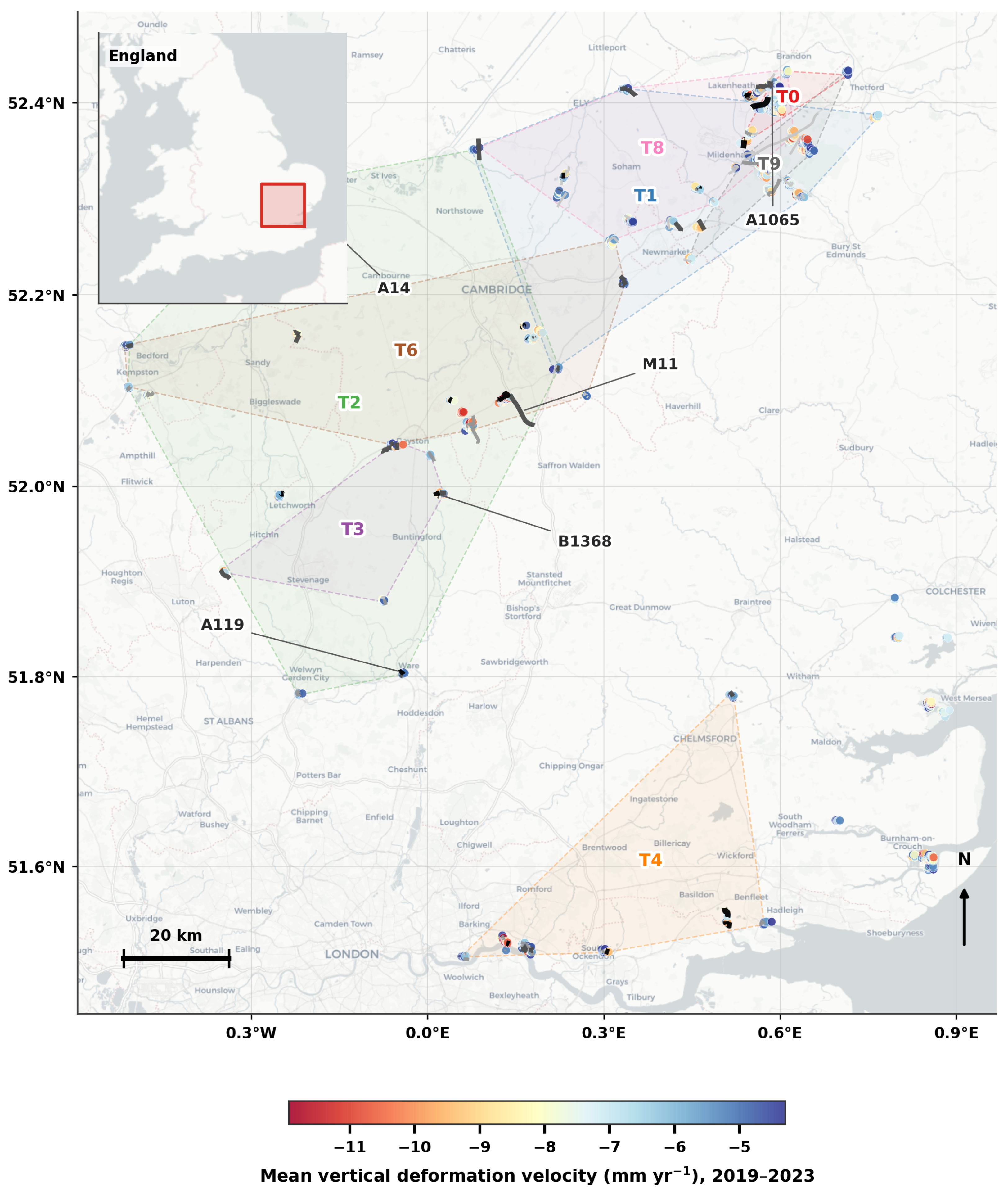
The proposed framework was evaluated using satellite-derived ground deformation observations and road infrastructure data from East Anglia, Eastern England. The study area covers approximately $100\times 100$ km and includes a mixture of urban centres, agricultural landscapes, river catchments, and nationally significant transport infrastructure (Figure 1). Major road corridors within the study area include sections of the M11 motorway, the A14 trunk road, the A119, A1065, and several secondary roads that provide an appropriate testbed for evaluating infrastructure-oriented deformation monitoring.

Ground deformation observations were obtained from the European Ground Motion Service (EGMS), which provides continent-wide measurements derived from multi-temporal Sentinel-1 Interferometric Synthetic Aperture Radar (InSAR) processing. The study utilised the mean vertical ground deformation velocity product for the 2019–2023 observation period, expressed in millimetres per year (mm/yr). This product was adopted deliberately rather than the alternative EGMS multi-temporal displacement time series: the transferability framework proposed in this study characterises source–target divergence through a single, well-understood environmental similarity measure, and extending this framework to multi-temporal data would introduce a second, temporal divergence dimension whose interaction with environmental divergence under joint spatiotemporal transfer is not yet established. Incorporating temporal transfer without first understanding how these two divergence sources jointly govern transfer reliability risks producing a reliability framework whose uncertainty quantification cannot itself be trusted, which would undermine the central contribution of this study. EGMS observations were pre-processed to remove invalid measurements, transformed into a common projected coordinate reference system for spatial analysis, and subsequently associated with environmental attributes used throughout the transfer-learning framework. Figure 1 illustrates the spatial distribution of deformation velocities across the study area.

Road infrastructure was extracted from the OpenStreetMap road network and processed to retain corridors relevant to regional transportation monitoring. Each road segment was spatially linked to nearby EGMS observations to enable corridor-level deformation assessment and subsequent reliability analysis. The resulting dataset comprises 140 named and unnamed road corridors that serve as the primary deployment units for prediction, validation, and reliability assessment.

To facilitate spatial transfer learning, the deformation observations were partitioned into a set of spatial monitoring tasks representing environmentally and geographically coherent regions. Each task functions as either a source or target domain during transfer learning, enabling systematic evaluation of cross-region knowledge transfer while preserving spatial independence between monitoring domains. The resulting task configuration, shown in Figure 1 provides the basis for the transferability analysis presented in the subsequent methodology.

4. Transferability-Aware Monitoring Framework

The proposed transferability-aware monitoring framework is designed to support deformation prediction in regions where observational coverage is sparse or unevenly distributed. The framework operates by partitioning the study area into spatially coherent monitoring tasks, identifying suitable source regions through transferability analysis, and exploiting transferable knowledge to improve prediction in target regions. By combining information derived from both local observations and environmentally similar source tasks, the framework enables the generation of spatially informed deformation estimates while reducing the risk of inappropriate knowledge transfer between dissimilar regions.

4.1. Framework Overview

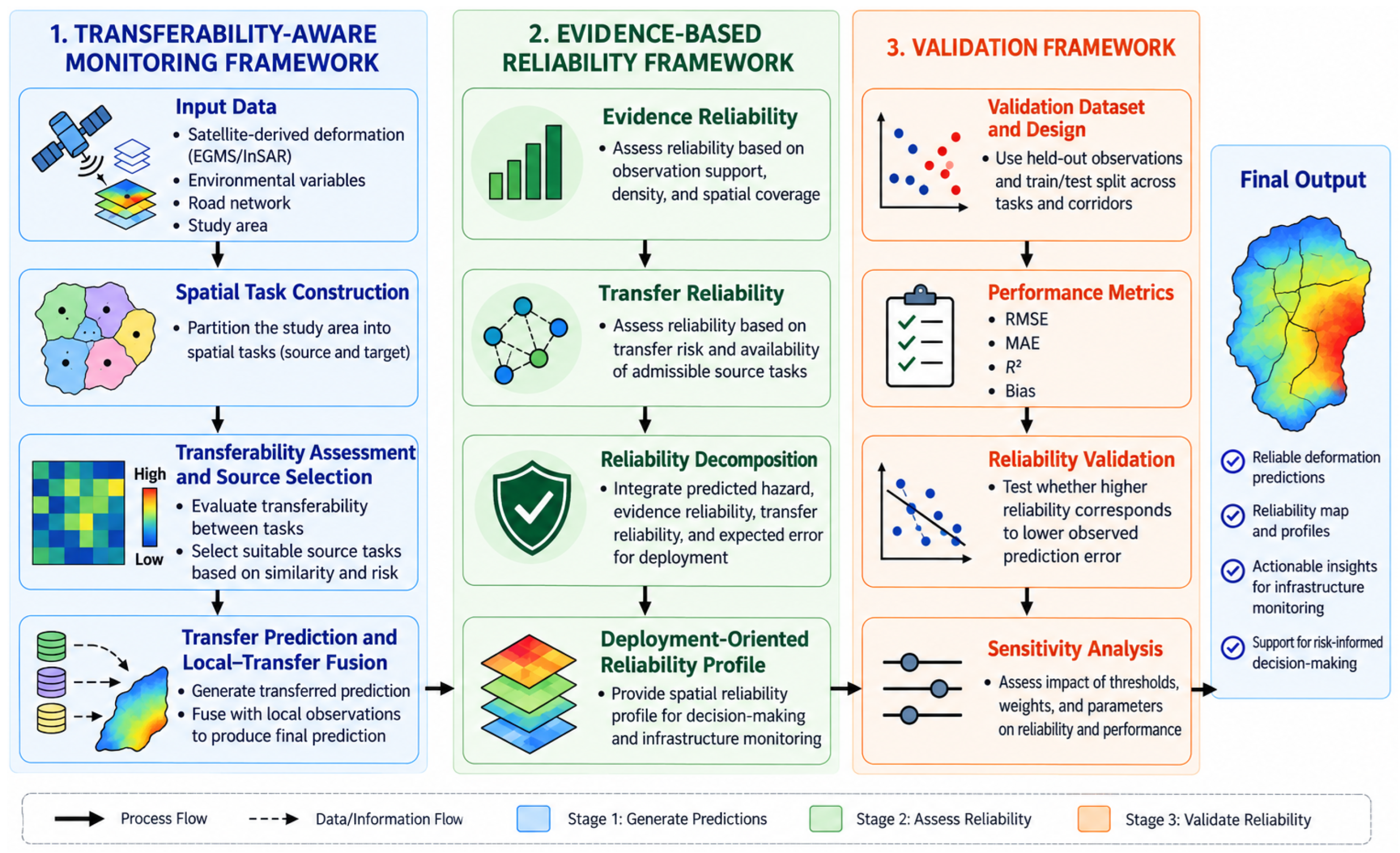
The proposed methodology supports reliable ground deformation monitoring in regions with sparse or unevenly distributed satellite observations by integrating spatial transfer learning with an evidence-based reliability assessment strategy across three sequential stages as illustrated in Figure 2. First, the Transferability-Aware Monitoring Framework constructs spatial monitoring tasks, identifies suitable knowledge sources through transferability assessment, and combines transferred predictions with local observations through a local–transfer fusion process. Second, the Evidence-Based Reliability Framework quantifies prediction trustworthiness from two complementary perspectives, evidence reliability, reflecting the strength of local observational support, and transfer reliability, reflecting the expected quality of transferred knowledge, and integrates these into a deployment-oriented reliability profile. Third, the Validation Framework assesses whether higher reliability classes correspond to lower observed prediction errors using held-out observations, producing deformation predictions accompanied by interpretable reliability information suitable for infrastructure monitoring and decision support.

4.2. Spatial Task Construction

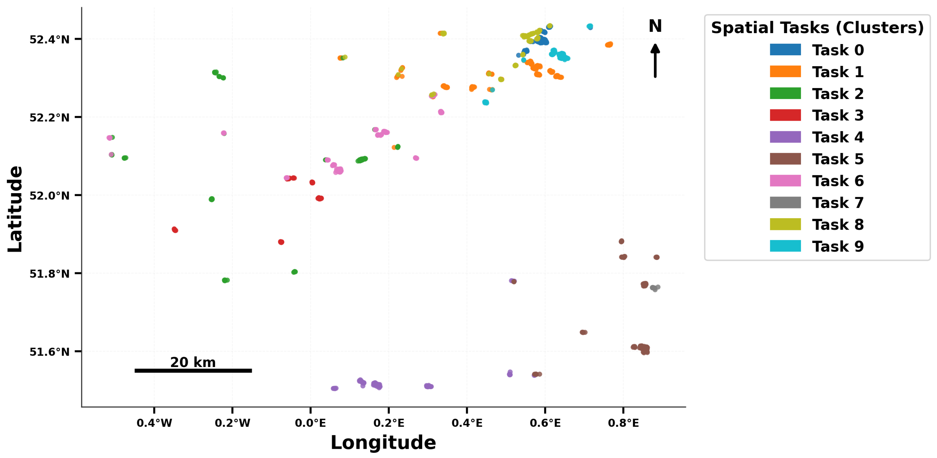
Tasks were constructed using a data-driven clustering strategy that jointly considers geographic location and environmental characteristics, producing ten spatially coherent monitoring domains that serve as transferable units of knowledge for subsequent source–target transfer learning experiments as illustrated in Figure 3. Let

$$\mathcal{D}={\left\{({\mathbf{x}}_i,y_i)\right\}}_{i=1}^N$$

(1)

denote the set of deformation observations, where N is the total number of observations, $y_i$ represents the observed ground deformation velocity, and ${\mathbf{x}}_i$ denotes the associated environmental attributes. For each observation, a spatial–environmental feature vector was constructed as

$${\mathbf{z}}_i={\left[{\lambda }_i,{\varphi }_i,e_i,w_i,u_i\right]}^{\top },$$

(2)

where ${\lambda }_i$ and ${\varphi }_i$ denote longitude and latitude, respectively, $e_i$ represents elevation, $w_i$ is the logarithmically transformed distance to the nearest water body, and $u_i$ is the logarithmically transformed distance to the nearest urban area. This compact feature vector was deliberately restricted to a small number of stable, low-noise geographic and topographic attributes for the specific purpose of spatial task construction: clustering on a minimal, well-behaved feature set produces geographically coherent and reproducible task partitions, whereas including high-dimensional or noisy environmental indices at this stage risks fragmenting otherwise contiguous regions. This clustering feature vector ${\mathbf{z}}_i$ is distinct from, and substantially smaller than, the environmental variable sets used in subsequent stages of the framework: transferability assessment (Section 4.3) is based on 21 environmental variables, and the local–transfer prediction models use 35 environmental variables, both of which incorporate vegetation, water, and climate indices in addition to the geographic attributes used here. These variables were selected to jointly represent the geographic and environmental conditions that may influence deformation behaviour and transferability between regions. To ensure that all variables contributed equally during clustering, each feature was standardised using z-score normalisation,

$${\tilde{z}}_{ij}={\displaystyle \frac{z_{ij}-{\mu }_j}{{\sigma }_j}},$$

(3)

where ${\mu }_j$ and ${\sigma }_j$ denote the mean and standard deviation of feature j, respectively.

Spatial tasks were then generated using K-means clustering [39], which partitions observations into K clusters by minimising the within-cluster sum of squared distances,

$$\underset{\mathcal{T}}{\min }{\displaystyle \sum _{k=1}^K}\sum _{{\mathbf{z}}_i\in T_k}{∥{\tilde{\mathbf{z}}}_i-{\mu }_k∥}_2^2,$$

(4)

where $T_k$ denotes the set of observations assigned to task k and ${\mu }_k$ denotes the corresponding cluster centroid. In this study, $K=10$ was adopted to provide a balance between environmental diversity across tasks and sufficient observational support within individual tasks. Because clustering solutions may vary owing to random initialisation, the task construction procedure was repeated across multiple clustering realisations. The stability of each partition was evaluated using the Adjusted Rand Index (ARI) [40], which measures the agreement between two cluster assignments while correcting for chance. For two partitions $P_a$ and $P_b$, the ARI is given by

$$\mathrm{ARI}={\displaystyle \frac{\mathrm{RI}-\mathbb{E}\left[\mathrm{RI}\right]}{\max \left(\mathrm{RI}\right)-\mathbb{E}\left[\mathrm{RI}\right]}},$$

(5)

where $\mathrm{RI}$ denotes the Rand Index. The final task configuration was selected as the clustering solution exhibiting the highest average agreement with all other candidate partitions,

$$P^{\ast }=\arg \underset{P_r}{\max }{\displaystyle \frac{1}{R-1}}{\displaystyle \sum _{\begin{array}{c}s=1\\ s\ne r\end{array}}^R}\mathrm{ARI}(P_r,P_s),$$

(6)

where R denotes the total number of clustering realisations. As illustrated in Figure 3, the resulting tasks form geographically contiguous regions while preserving environmental heterogeneity across the study area. This structure provides a suitable basis for assessing transferability between spatial domains and enables the systematic evaluation of source–target knowledge transfer in subsequent stages of the framework.

4.3. Transferability Assessment and Source Selection

Following task construction, the suitability of knowledge transfer between tasks was evaluated using complementary environmental and structural similarity measures. Unlike the compact five-variable feature vector used for task construction (Equation (2)), transferability assessment draws on a substantially larger set of 21 environmental variables, comprising mean, standard deviation, and trend statistics for NDVI, SAVI, NDWI, MNDWI, precipitation, and temperature, together with elevation and distance to water and urban areas, in order to characterise the full distributional structure of each environmental attribute rather than a single representative value. For a target task $T_j$, transferability was assessed against all candidate source tasks $T_i$, after which the most compatible sources were retained for transfer learning. Environmental similarity was quantified using the first Wasserstein distance (Earth Mover’s Distance) [41]. Let $f_m^{\left(i\right)}$ and $f_m^{\left(j\right)}$ denote the distributions of environmental feature m within tasks $T_i$ and $T_j$, respectively. The feature–space distance between two tasks was computed as

$$D_F(T_i,T_j)={\displaystyle \frac{1}{M}}{\displaystyle \sum _{m=1}^M}{W}_1\left(f_m^{\left(i\right)},f_m^{\left(j\right)}\right),$$

(7)

where M denotes the number of environmental variables and $W_1(·)$ represents the Wasserstein distance. To capture differences in spatial organisation, each task was additionally represented as a k-nearest-neighbour graph constructed from geographic coordinates. The graph Laplacian spectrum provides a compact description of structural connectivity and spatial geometry [42]. Let ${\mathit{\lambda }}^{\left(i\right)}$ and ${\mathit{\lambda }}^{\left(j\right)}$ denote the normalised Laplacian eigenvalue vectors of tasks $T_i$ and $T_j$. The spectral distance was defined as

$$D_S(T_i,T_j)={\displaystyle \frac{1}{K}}{∥{\mathit{\lambda }}^{\left(i\right)}-{\mathit{\lambda }}^{\left(j\right)}∥}_2,$$

(8)

where K is the common spectral truncation length. Candidate source tasks were subsequently ranked according to increasing task distance, such that environmentally and structurally similar tasks were preferred over dissimilar ones.

4.4. Transfer Prediction and Local–Transfer Fusion

For each admissible source–target pair identified during transferability assessment, deformation predictions were generated using both transferred and local information. Let $T_s$ denote the selected source task and $T_t$ the corresponding target task. A transfer model was trained on observations from $T_s$ and applied to $T_t$, while a local model was trained using observations available within $T_t$. Both models were implemented using Random Forest regression [43]. Given a feature vector $\mathbf{x}$, the transferred and local predictions are expressed as

$${\widehat{y}}_{\mathrm{transfer}}=f_s\left(\mathbf{x}\right),{\widehat{y}}_{\mathrm{local}}=f_t\left(\mathbf{x}\right),$$

(9)

where $f_s(·)$ and $f_t(·)$ denote source-trained and target-trained Random Forest models, respectively. In the validation experiment, the local model was trained using a subset of target observations and evaluated on held-out target observations. The local contribution was controlled by the amount of observational support available within the target task. Let $n_t$ denote the number of target observations. A normalised local reliability score was computed as

$$L_t=0.2+0.8\left({\displaystyle \frac{n_t-n_{\min }}{n_{\max }-n_{\min }+ϵ}}\right),$$

(10)

where $n_t$ is the number of observations available for the target task, $n_{\min }$ and $n_{\max }$ are the minimum and maximum target sample counts among the admissible transfers, and $ϵ$ is a small constant introduced to avoid division by zero. The observed sample counts are first normalised to reflect the relative strength of local observational evidence and are then rescaled to the interval $[0.2,1]$. The lower bound of $0.2$ prevents the local component from receiving zero reliability in sparsely sampled target tasks, thereby preserving a minimum contribution from local observations while allowing the remaining reliability to vary according to the available evidence. Transfer reliability was derived from the transfer-risk score associated with the selected source–target pair. Let $r_{st}\in [0,1]$ denote the transfer-risk score. The transfer reliability was defined as

$$T_{st}=1-r_{st}.$$

(11)

Initial local and transfer weights were then computed as

$$w_L^{\left(0\right)}={\displaystyle \frac{L_t}{L_t+T_{st}+ϵ}},w_T^{\left(0\right)}={\displaystyle \frac{T_{st}}{L_t+T_{st}+ϵ}}.$$

(12)

To further reduce the influence of risky transfers, the transfer weight was penalised by the transfer-risk score,

$${\tilde{w}}_T=w_T^{\left(0\right)}(1-r_{st}),$$

(13)

and the removed transfer contribution was reassigned to the local component,

$${\tilde{w}}_L=w_L^{\left(0\right)}+\left(w_T^{\left(0\right)}-{\tilde{w}}_T\right).$$

(14)

The adjusted weights were finally renormalised as

$$w_T={\displaystyle \frac{{\tilde{w}}_T}{{\tilde{w}}_T+{\tilde{w}}_L+ϵ}},w_L={\displaystyle \frac{{\tilde{w}}_L}{{\tilde{w}}_T+{\tilde{w}}_L+ϵ}}.$$

(15)

The final fused prediction was obtained as

$${\widehat{y}}_{\mathrm{fused}}=w_L{\widehat{y}}_{\mathrm{local}}+w_T{\widehat{y}}_{\mathrm{transfer}}.$$

(16)

This formulation allows transferred information to contribute more strongly when transfer risk is low, while increasing the influence of local predictions when transfer risk is high or when sufficient target observations are available.

4.5. Multi-Source Ensemble Fusion

As an alternative to selecting a single source task, predictions for a target task $T_j$ may instead be constructed by combining multiple admissible source tasks. For each candidate source $T_i$, a risk-adjusted transfer score was computed as

$${\mathrm{score}}_i={\mathrm{RMSE}}_i^{\exp }+{\lambda }_{\mathrm{risk}}\mathrm{corridor}\_{\mathrm{risk}}_i,$$

(17)

where ${\mathrm{RMSE}}_i^{\exp }$ denotes the expected transfer RMSE for source $T_i$, $\mathrm{corridor}\_{\mathrm{risk}}_i$ denotes the corridor-level transfer risk score associated with that source–target pair, and ${\lambda }_{\mathrm{risk}}=0.5$ controls the degree of risk aversion applied when ranking candidate sources. Lower scores indicate more favourable sources. Source tasks were ranked by ${\mathrm{score}}_i$, and predictions were combined using weights that decreased monotonically with this score, such that sources with lower expected error and lower corridor-level transfer risk received proportionally greater influence in the final ensemble prediction; weights were normalised to sum to 1 within each target task (Section 6.3 reports the empirical relationship between source cost and assigned weight). The full multi-source ensemble retained all admissible sources for a given target, while the sparse multi-source ensemble retained only the $K=3$ most favourably ranked sources, corresponding to the “top-weighted” sources reported in the Results. The final multi-source prediction was obtained as a weighted average of the individual source-model predictions,

$${\widehat{y}}_{\mathrm{multi}}={\displaystyle \sum _{i=1}^K}{w}_i{\widehat{y}}_i,$$

(18)

where ${\widehat{y}}_i$ denotes the prediction obtained from a Random Forest model trained on source task $T_i$ and applied to the target task, and $w_i$ denotes the normalised weight assigned to source $T_i$. This formulation allows multiple heterogeneous source tasks to contribute to a single prediction while systematically down-weighting sources associated with higher expected error or corridor-level transfer risk.

4.6. Prediction Backbone Selection

Random Forest was adopted as the prediction backbone owing to its established robustness under sparse, nonlinear, and heterogeneous spatial data, and its established use in prior satellite-derived deformation modelling [9,10,11]. To verify that this choice was not arbitrary, five additional backbones were evaluated under an identical leakage-safe, domain-held-out protocol: Extra Trees, Gradient Boosting, XGBoost, Gaussian Process regression, and a lightweight feed-forward neural network (multi-layer perceptron). Every model was trained on the same 35-variable environmental feature set (Section 4.3) and evaluated using the same eight leave-one-domain-out folds so that differences in performance reflect the choice of backbone rather than differences in features, preprocessing, or evaluation protocol. The Gaussian Process baseline uses an RBF kernel over the full environmental feature space and should be distinguished from classical spatial Kriging, which is typically formulated using only spatial coordinates and an explicitly fitted variogram; similarly, the neural network baseline is a feed-forward multi-layer perceptron rather than a convolutional architecture since the per-observation tabular structure of the dataset does not admit a direct convolutional formulation without substantial restructuring into spatial image patches. Results of this comparison are reported in Section 6.4.

5. Evidence-Based Reliability Framework

The practical value of deformation predictions depends not only on their accuracy but also on the confidence that can be placed in them. In data-sparse monitoring environments, prediction uncertainty may arise from limited observational support, incomplete spatial coverage, and the transfer of knowledge across heterogeneous regions. Consequently, reliable deployment requires an assessment framework capable of quantifying the strength of available evidence and the trustworthiness of transferred information. To address this need, the proposed evidence-based reliability framework evaluates prediction confidence from complementary observational and transfer-learning perspectives and integrates them into a deployment-oriented reliability profile.

5.1. Reliability Concept

Reliability is defined as the degree to which a deformation prediction is supported by available evidence and transferable knowledge, quantified through two complementary components: evidence reliability $R_E$, which reflects the strength of local observational support, and transfer reliability $R_T$, which reflects the expected trustworthiness of transferred knowledge. These components are preserved as independent descriptors rather than combined into a single score so that the origin of uncertainty remains transparent to the user. Let

$$\mathbf{R}=\left(R_E,R_T\right),$$

(19)

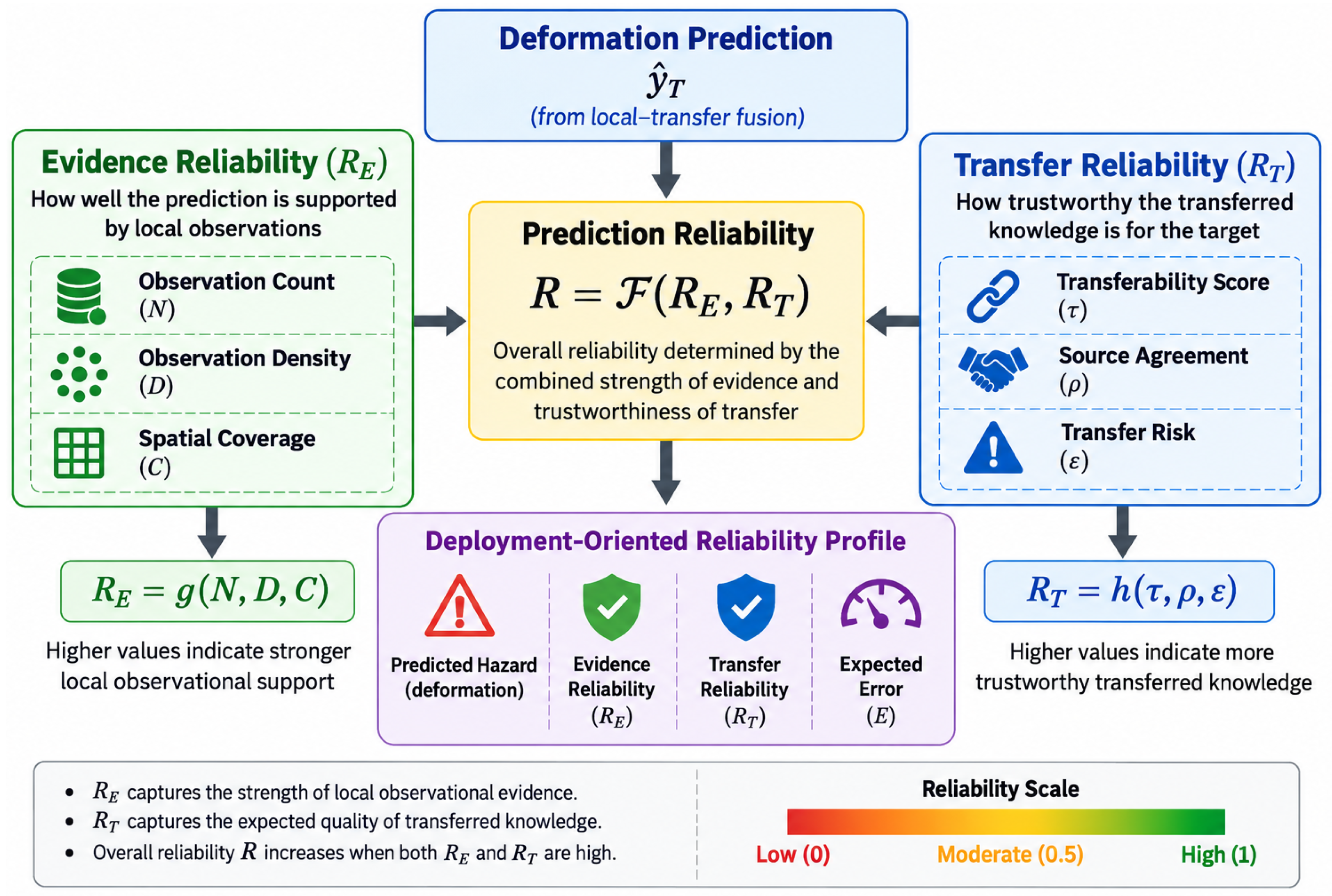
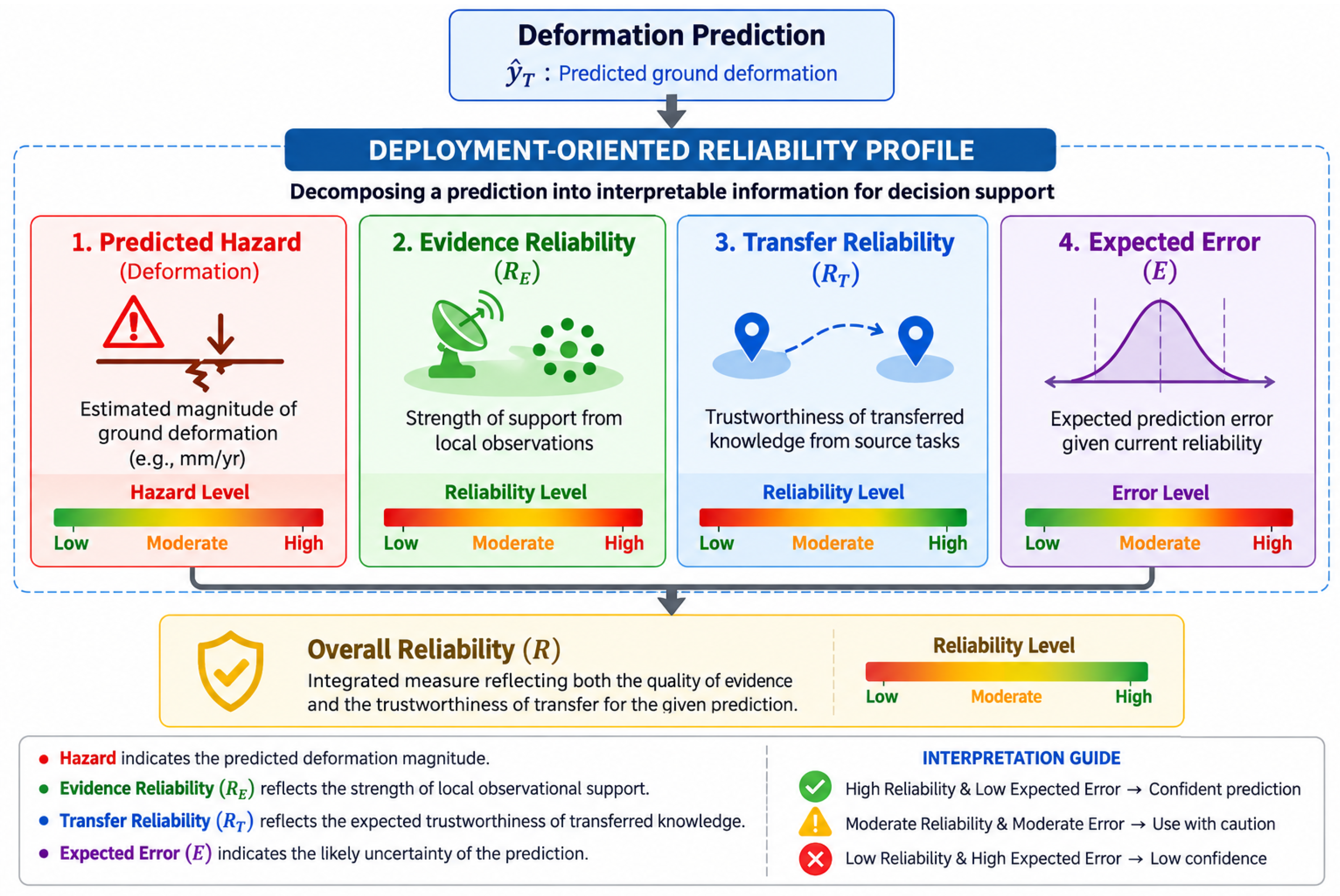
denote the reliability profile associated with a prediction, where each component is evaluated independently using the rule-based procedures described in the following subsections and reported alongside the predicted deformation hazard and expected prediction error as illustrated in Figure 4.

5.2. Evidence Reliability

Evidence reliability quantifies the extent to which a deformation prediction is supported by local observational evidence. In the proposed framework, reliability is evaluated using three complementary indicators that characterise the availability and spatial representativeness of satellite observations within each monitoring task: observation count, observation density, and spatial coverage. Rather than combining these indicators through a weighted aggregation, evidence reliability is determined using a rule-based classification procedure that reflects the implemented workflow. Let $T_t$ denote a monitoring task containing a set of deformation observations

$${\mathcal{D}}_t={\left\{({\mathbf{x}}_i,y_i)\right\}}_{i=1}^{N_t},$$

(20)

where $N_t=\left|{\mathcal{D}}_t\right|$ denotes the number of observations available within the task. Observation density is defined as

$${\rho }_t={\displaystyle \frac{N_t}{A_t}},$$

(21)

where $A_t$ is the spatial extent of the monitoring task. Spatial coverage measures the proportion of the task area represented by valid deformation observations,

$$C_t={\displaystyle \frac{A_{\mathrm{obs}}}{A_t}},$$

(22)

where $A_{\mathrm{obs}}$ denotes the area effectively supported by observations. For each monitoring task, the three indicators were compared with the empirical distributions obtained across all tasks. Let $Q_p(·)$ denote the p-th empirical quantile. Evidence reliability was assigned according to

$$R_E\left(T_t\right)=\left\{\begin{array}{cc}\mathrm{High},\hfill & N_t\ge Q_{0.75}\left(N\right),{\rho }_t\ge Q_{0.75}\left(\rho \right),C_t\ge Q_{0.75}\left(C\right),\hfill \\ \mathrm{Medium},\hfill & N_t\ge Q_{0.50}\left(N\right),{\rho }_t\ge Q_{0.50}\left(\rho \right),C_t\ge Q_{0.50}\left(C\right)\hfill \\ \mathrm{Low},\hfill & \mathrm{otherwise}.\hfill \end{array}\right.$$

(23)

This formulation classifies evidence reliability directly from the observed level of local data support without requiring subjective weighting coefficients. Monitoring tasks containing numerous, spatially dense, and well-distributed observations are therefore assigned higher evidence reliability than tasks characterised by sparse or uneven observational support. The resulting ordinal reliability classes provide an interpretable measure of the strength of local evidence and constitute the first component of the proposed reliability framework.

5.3. Transfer Reliability

Transfer reliability quantifies the expected trustworthiness of knowledge transferred from source tasks to a target task. Unlike evidence reliability, which reflects the strength of local observational support, transfer reliability characterises the expected quality of transferred information based on the transferability analysis. The proposed framework considers two complementary indicators: the estimated transfer risk associated with each source–target pair and the availability of admissible source tasks capable of contributing transferable knowledge. Let $r_{ij}\in [0,1]$ denote the transfer-risk score between source task $T_i$ and target task $T_j$, where smaller values indicate lower expected transfer uncertainty. Let $M_j$ denote the number of admissible source tasks identified for target task $T_j$. To ensure comparability across monitoring tasks, both indicators were converted to percentile ranks,

$$p_r=1-{\mathrm{rank}}_{\mathrm{pct}}\left(r_{ij}\right),p_M={\mathrm{rank}}_{\mathrm{pct}}\left(M_j\right),$$

(24)

where ${\mathrm{rank}}_{\mathrm{pct}}(·)$ denotes the empirical percentile rank. Lower transfer risk therefore corresponds to higher reliability, while target tasks with a greater number of suitable source tasks receive stronger transfer support. The overall transfer score was computed using the rule implemented in the proposed framework,

$$S_T=0.7p_r+0.3p_M,$$

(25)

where $p_r$ and $p_M$ denote the percentile-based transfer-risk and source-availability components, respectively. The structure of this formulation reflects an evidence-based prioritisation of the two contributing indicators. Transfer risk $p_r$ receives the greater weight of $0.7$ because it provides the most direct indication of the expected trustworthiness of transferred predictions: a high transfer-risk score indicates that the source–target pair is likely to produce unreliable knowledge transfer regardless of how many alternative sources are available. Source availability $p_M$ receives the complementary weight of $0.3$ because the number of admissible source tasks strengthens transfer confidence when multiple compatible donors agree, but cannot compensate for high transfer risk in any individual pair. Both components are expressed as percentile ranks prior to aggregation, ensuring that the combined score $S_T$ is robust to skewed distributions and comparable across monitoring tasks with different absolute sample counts. The weighting coefficients $0.7$ and $0.3$ were specified a priori as transparent design choices grounded in this evidence-based ordering of indicator importance rather than determined through parameter optimisation. To assess the sensitivity of this choice, the transfer-risk weight was varied systematically from 0 to 1 in increments of 0.05, and the resulting transfer score was tested against corridor-level validation RMSE at each setting ($n=46$ corridors with held-out validation observations). No tested weighting, including the adopted 0.7/0.3 setting ($\rho =-0.109$, $p=0.470$), achieved statistical significance (all $p>0.30$ across the full sweep), and the strongest observed association ($\rho =-0.154$, $p=0.308$, at a risk weight of 0) was itself non-significant. This indicates that the available corridor-level validation data do not support the identification of a statistically superior alternative weighting, and is consistent with treating the 0.7/0.3 coefficients as a transparent, evidence-motivated design choice rather than a value determined or determinable through post-hoc optimisation on this dataset.

For deployment, the continuous transfer score was converted into ordinal reliability classes using empirical tertiles,

$$R_T=\left\{\begin{array}{cc}\mathrm{High},\hfill & S_T\ge Q_{0.66}\left(S_T\right),\hfill \\ \mathrm{Medium},\hfill & Q_{0.33}\left(S_T\right)\le S_T{Q}_{0.66}\left(S_T\right),\hfill \\ \mathrm{Low},\hfill & S_T{Q}_{0.33}\left(S_T\right),\hfill \end{array}\right.$$

(26)

where $Q_{0.33}(·)$ and $Q_{0.66}(·)$ denote the 33rd and 66th percentiles of the transfer-score distribution across all monitoring tasks. Empirical tertiles were adopted rather than fixed absolute thresholds for two reasons. First, the resulting classification is fully data-adaptive: the boundaries are determined by the observed distribution of $S_T$ across the study area and therefore adjust automatically to the range of transfer conditions present in any given deployment context, without requiring prior knowledge of what constitutes a high or low transfer score in absolute terms. Second, tertile-based classification guarantees that the three reliability classes are approximately balanced in size, preventing degenerate outcomes in which nearly all corridors collapse into a single class. Consequently, tasks exhibiting lower transfer risk and stronger transfer support are assigned higher transfer reliability, forming the second component of the proposed deployment-oriented reliability framework.

5.4. Deployment-Oriented Reliability Decomposition

For operational monitoring applications, a deformation prediction alone provides limited information regarding its suitability for decision-making. Consequently, the proposed framework decomposes each prediction into a deployment-oriented reliability profile that combines predicted deformation hazard with complementary reliability indicators. As illustrated in Figure 5, the resulting profile separates prediction magnitude from prediction confidence, enabling users to distinguish between areas exhibiting significant deformation and areas for which the supporting evidence is sufficiently reliable. Let

$$\Pi =\left\{H,R_E,R_T,E\right\},$$

(27)

denote the deployment-oriented reliability profile associated with a prediction, where H represents the predicted deformation hazard, $R_E$ denotes evidence reliability, $R_T$ denotes transfer reliability, and E denotes the expected prediction error. The predicted hazard is represented by the absolute magnitude of the final fused prediction, $|{\widehat{y}}_{\mathrm{fused}}|$, where ${\widehat{y}}_{\mathrm{fused}}$ is obtained from the local–transfer fusion procedure described in the preceding section. Deformation hazard was subsequently categorised into four ordinal classes using a data-calibrated rule that combines the absolute predicted velocity magnitude with the proportion of severely-deforming points observed within each corridor, rather than fixed absolute velocity thresholds. Let $Q_{50}\left(H\right)$, $Q_{75}\left(H\right)$, and $Q_{90}\left(H\right)$ denote the 50th, 75th, and 90th percentiles of the absolute predicted velocity magnitude across all monitored corridors, and let $F_C$ and $F_{HC}$ denote, respectively, the proportion of points within a corridor classified as critical and the proportion classified as high-or-critical under a point-level threshold applied prior to corridor-level aggregation. The hazard class was then defined as

$$H_{\mathrm{class}}=\left\{\begin{array}{cc}\mathrm{Critical},\hfill & H\ge Q_{90}\left(H\right)\mathrm{or}{F}_C\ge 0.30,\hfill \\ \mathrm{High},\hfill & H\ge Q_{75}\left(H\right)\mathrm{or}{F}_{HC}\ge 0.50,\hfill \\ \mathrm{Moderate},\hfill & H\ge Q_{50}\left(H\right)\mathrm{or}{F}_{HC}\ge 0.20,\hfill \\ \mathrm{Low},\hfill & \mathrm{otherwise}.\hfill \end{array}\right.$$

(28)

This calibrated formulation was adopted in place of fixed absolute velocity thresholds for two reasons. First, it adapts the classification to the empirical distribution of predicted velocities within the study area, avoiding the imposition of an external threshold that may not reflect the actual range or clustering of predictions produced by the framework. Second, the disjunctive combination with corridor-level severity fractions ($F_C$, $F_{HC}$) ensures that a corridor is flagged as high-hazard if either its peak predicted velocity is extreme relative to the rest of the study area, or a substantial proportion of its individual observation points exhibit severe deformation, rather than relying on a single peak-velocity statistic alone. We note that this calibrated rule, rather than a fixed 8/5/2 mm/yr threshold set, is the classification actually applied throughout this study; an earlier description of this equation in terms of fixed absolute thresholds did not accurately reflect the implemented methodology, and has been corrected here. Rather than estimating uncertainty through an analytical function, the expected prediction error is derived empirically from the validation experiments. Let $E_E\left(R_E\right)$ denote the average validation error associated with each evidence reliability class, and let $E_T\left(R_T\right)$ denote the corresponding average validation error for each transfer reliability class. The expected prediction error is defined as

$$E=\max \left[E_E\left(R_E\right),E_T\left(R_T\right)\right],$$

(29)

where $E_E\left(R_E\right)$ and $E_T\left(R_T\right)$ denote the mean validation RMSE observed for the evidence and transfer reliability classes assigned to the prediction, respectively. The structure of this formulation reflects a deliberate conservative design principle: rather than averaging the two reliability-class errors or selecting one arbitrarily, the maximum is taken so that the reported expected error is always governed by whichever source of uncertainty is the more severe. This is appropriate because evidence reliability and transfer reliability capture distinct and largely independent origins of prediction uncertainty. A prediction may be supported by strong local observational evidence yet originate from a high-risk transfer, or conversely may benefit from a low-risk transfer while being situated in a data-sparse corridor with low evidence reliability. In either case, the dominant source of uncertainty should determine the expected error communicated to the user. Taking the maximum therefore prevents the framework from underreporting uncertainty by allowing a favourable reliability class on one dimension to mask an unfavourable class on the other. The resulting expected error is empirically grounded, derived directly from held-out validation performance rather than from a parametric uncertainty model, and is conservatively calibrated in the sense that the mean expected error band exceeded the mean observed validation RMSE across the study area. The deployment profile defined in Equation (27) therefore provides a multidimensional description of prediction behaviour by combining hazard severity, evidence reliability, transfer reliability, and the expected prediction error, enabling users to assess both the severity of predicted deformation and the confidence associated with each prediction when supporting deployment decisions.

For practical deployment, the reliability profile may be represented through categorical reliability maps, corridor-level summaries, or infrastructure prioritisation tables. As shown in Figure 5, the combined presentation of hazard, reliability, and expected error provides a transparent basis for prioritising inspection, maintenance, and monitoring activities within infrastructure management systems.

5.5. Validation Framework

Validation in this study is internal to the EGMS observational record: predictive performance and reliability behaviour were assessed against EGMS observations withheld from training, rather than against an independent measurement technology such as GNSS or levelling. This validation strategy tests whether the proposed framework generalises to unseen EGMS observations and whether reliability estimates track realised prediction error within this observational record; it does not, and is not intended to, assess whether the underlying EGMS product itself is accurate relative to ground-based geodetic measurement. The proposed framework was evaluated using held-out observations that were excluded from model training and transfer-learning procedures. Validation was designed to assess both predictive performance and the effectiveness of the proposed reliability measures. For each target task, transferred and fused predictions were compared with the observed deformation values to examine the relationship between the estimated reliability and the realised prediction errors. Predictive performance was assessed using the root mean square error (RMSE) and mean absolute error (MAE), which provide complementary measures of prediction accuracy. In addition to conventional accuracy assessment, the proposed reliability framework was evaluated by testing whether predictions assigned higher reliability consistently exhibited lower observed errors. Prediction errors were therefore analysed across the low-, medium-, and high-reliability classes for both the evidence reliability and transfer reliability measures. A reliable framework is expected to demonstrate a monotonic relationship in which higher reliability classes correspond to lower validation errors. This validation strategy directly assesses whether the proposed reliability measures provide meaningful indicators of prediction quality during deployment. Collectively, these validation experiments assess predictive performance, reliability behaviour, and the practical suitability of the proposed framework for deployment-oriented ground deformation monitoring.

6. Results

This section presents the empirical findings of the proposed transferability-aware monitoring framework applied to EGMS vertical deformation observations across a 100 km × 100 km tile covering East Anglia and surrounding road infrastructure. Results are organised to follow the three sequential stages of the framework. Section 6.1 characterises the spatial transferability structure of the eight monitoring tasks and the admissibility of source–target pairs. Section 6.2 evaluates cross-task transfer prediction performance across three prediction strategies and compares their accuracy against held-out observations. Section 6.6 examines the relationship between divergence-based transferability measures and realised prediction error, including directional asymmetry effects. Section 6.7 and Section 6.8 present the evidence and transfer reliability assessments at corridor level and examine whether reliability classes correspond to differences in observed prediction error. Section 6.9 reports the overall reliability validation, including expected error band coverage, and Section 6.10 translates the combined reliability profiles into deployment-oriented monitoring recommendations for 140 named and unnamed road corridors, with particular reference to nationally significant infrastructure including the M11 motorway, A14 trunk road, and A119 Ware Road.

6.1. Spatial Transferability Analysis

A total of 815 EGMS vertical deformation observations were partitioned into ten spatially coherent monitoring tasks using stability-selected K-means clustering ($K=10$) applied to geographic coordinates, elevation, and proximity-to-water and proximity-to-urban features. Partition stability, evaluated across nine initialisations using the Adjusted Rand Index, yielded a mean pairwise ARI of 0.90 (range: 0.72–0.98), confirming robust task boundaries. Two of the ten tasks (Tasks 5 and 7) were subsequently excluded from the transfer learning analysis because they contained insufficient observations to satisfy the admissibility criteria, leaving eight tasks available for cross-task transfer experiments (range: 49–173 observations per task).

Pairwise transferability was assessed using feature–space divergence (mean Wasserstein distance across 21 environmental variables; range: 0.341–2.257) and graph Laplacian spectral divergence (range: 0.047–0.463). Source selection retained 38 admissible source–target pairs across seven target tasks. Task 4 received no eligible sources, reflecting genuine environmental isolation from all candidate regions. Task-level results are summarised in

Table 1. Spatial transferability summary by monitoring task.

Task	N	Sources	Top Pair	Exp. RMSE (mm/yr)	Risk Class
0	153	7	T8 → T0	1.344	Medium
1	173	6	T8 → T1	1.683	High
2	80	2	T9 → T2	2.738	Medium
3	49	7	T0 → T3	1.804	Medium
4	70	0	—	—	—
6	106	4	T9 → T6	2.071	Medium
8	79	5	T3 → T8	1.992	Low
9	105	7	T0 → T9	2.090	High

.

6.2. Cross-Task Transfer Performance

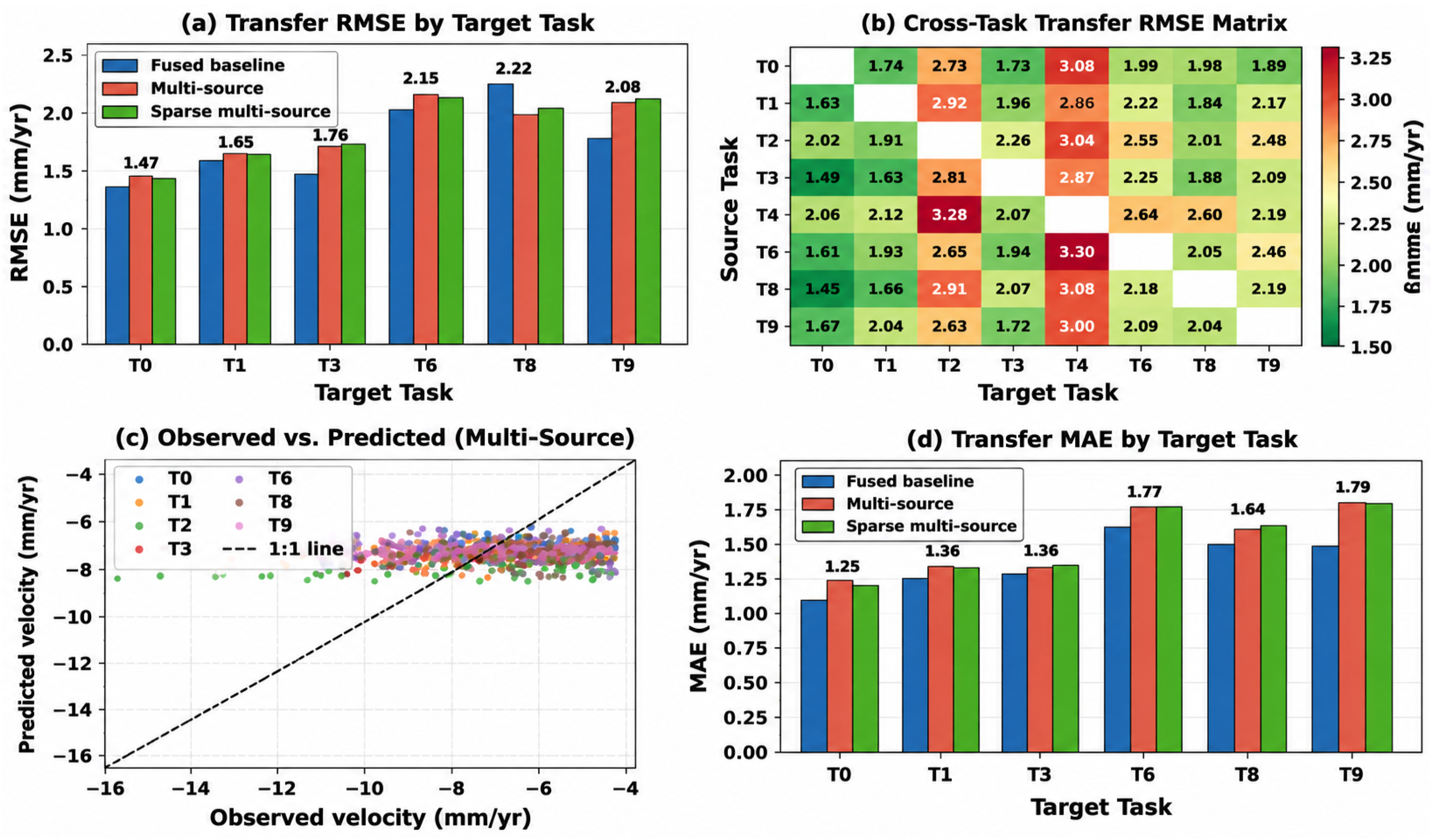
Cross-task transfer performance was evaluated across all admissible source–target pairs using three prediction strategies: a local–transfer fused baseline, a full multi-source ensemble, and a sparse multi-source ensemble retaining up to three top-weighted sources. Overall, the fused baseline achieved the lowest mean RMSE (1.720 mm/yr, MAE: 1.353 mm/yr), outperforming both the full multi-source ensemble (RMSE: 1.819 mm/yr) and the sparse variant (RMSE: 1.819 mm/yr), indicating that selective single-source fusion is more effective than averaging across multiple heterogeneous donors in this geotechnical setting.

Performance varied markedly across target tasks (Figure 6). Task 0, characterised by the highest environmental similarity to its top donor (T8, $D_F=0.341$), achieved the lowest transfer RMSE (1.378 mm/yr), while Task 2, the most environmentally isolated target, produced the highest error (2.656 mm/yr). Task 2 is a notable case in this respect: although its highest-ranked candidate source (T9) achieved a favourable risk profile relative to several accepted pairs elsewhere in the study, it did not satisfy the framework’s risk-acceptance criterion for transfer, and no fused baseline was therefore computed for this task. This reflects the framework’s decision logic correctly declining an available but insufficiently reliable transfer source, rather than a shortage of underlying observational data (Task 2’s total of 80 observations is comparable to several tasks with an accepted fused baseline, such as Task 8 at 79 and Task 3 at 49). The directional transfer RMSE matrix (Figure 6b) reveals consistent source asymmetry: Task 8 was the most transferable source, consistently achieving low RMSE when applied to Tasks 0 (1.455 mm/yr), 1 (1.663 mm/yr), and 3 (2.072 mm/yr), whereas Task 4 was the least transferable, producing RMSE values exceeding 3.000 mm/yr in five of seven target tasks. The observed-versus-predicted scatter (Figure 6c) reveals a systematic compression bias, which we quantify directly: across the 88 held-out validation points, the standard deviation of predicted absolute velocity (0.514 mm/yr) was only 29% of the standard deviation of observed absolute velocity (1.766 mm/yr), and this compression was more pronounced at corridor level (predicted std 0.494 mm/yr versus observed std 2.011 mm/yr, a ratio of 25%). The predicted range (2.44 mm/yr, spanning 5.66–8.10 mm/yr) covered only a third of the observed range (7.10 mm/yr, spanning 4.40–11.50 mm/yr), reflecting the inherent smoothing effect of Random Forest regression under cross-domain conditions. We report the consequences of this compression for hazard classification accuracy in Section 6.11. Task-level performance metrics are summarised in

Table 2. Task-level transfer performance. RMSE and MAE are reported in mm/yr. Fused: local–transfer fusion; MS: multi-source ensemble; SMS: sparse multi-source ensemble. Task 2 has no fused baseline because none of its candidate source tasks satisfied the framework’s risk-acceptance criterion for transfer (Section 6.2), despite Task 2’s total observation count (N = 80) being comparable to several tasks that do have a fused baseline.

Task	N	Fused		MS		SMS
		RMSE	MAE	RMSE	MAE	RMSE	MAE
T0	153	1.378	1.105	1.470	1.249	1.444	1.210
T1	173	1.597	1.273	1.653	1.353	1.638	1.357
T2	80	—	—	2.656	2.229	2.671	2.234
T3	49	1.460	1.302	1.716	1.340	1.757	1.364
T6	106	1.970	1.621	2.146	1.762	2.143	1.766
T8	79	2.221	1.501	1.936	1.600	1.991	1.644
T9	105	1.770	1.487	2.072	1.789	2.081	1.787
Mean	—	1.733	1.382	1.950	1.618	1.961	1.623

.

6.3. Multi-Source Ensemble Composition

Table 3. Sparse multi-source ensemble composition (top three retained sources per target task). Weights are normalised to sum to 1 within each target task.

Target	Source	Exp. RMSE (mm/yr)	Corridor Risk	Weight
T0	T8	1.319	0.642	0.232
T0	T3	1.577	0.435	0.170
T0	T9	1.563	0.583	0.151
T1	T8	1.679	0.702	0.216
T1	T3	1.884	0.377	0.199
T1	T9	1.820	0.652	0.171
T2	T9	2.763	0.472	0.371
T2	T0	2.667	0.721	0.350
T2	T8	2.776	0.732	0.279
T3	T0	1.801	0.510	0.190
T3	T9	1.886	0.368	0.185
T3	T8	1.966	0.434	0.147
T6	T9	2.066	0.541	0.338
T6	T8	2.161	0.687	0.241
T6	T4	2.449	0.184	0.224
T8	T3	2.000	0.409	0.240
T8	T9	1.920	0.579	0.237
T8	T4	2.149	0.328	0.193
T9	T0	2.102	0.703	0.181
T9	T3	2.310	0.428	0.157
T9	T4	2.437	0.177	0.157

reports the composition of the sparse multi-source ensemble for each target task, showing the three retained source tasks, their expected transfer RMSE, corridor-level transfer risk, an aggregate source cost combining these two indicators, and the resulting normalised ensemble weight. Weight assignment was monotonically related to source cost: sources with lower expected RMSE and lower corridor-level transfer risk received a higher share of the ensemble weight, and this relationship was strong (Pearson $r=0.96$ between a candidate inverse-cost weighting transform and the weights actually assigned) without corresponding to a single simple closed-form expression, reflecting additional calibration applied during weight normalisation. Across all seven target tasks, Task 8 and Task 9 were the most frequently retained sources, consistent with their favourable transfer-risk profiles reported in Section 6.2, while the weight distribution within each ensemble was moderately concentrated rather than uniform: the top-ranked source received a mean of 25.7% of the total ensemble weight across target tasks, compared with an equal-weight baseline of 33.3% for a three-source ensemble, indicating that the fusion strategy meaningfully discriminated between sources of differing reliability rather than defaulting to an equal-weighted average.

6.4. Prediction Backbone Comparison

To verify that Random Forest was a suitable choice of prediction backbone rather than an unexamined default, the same fused local–transfer prediction task was repeated using five additional regression backbones, under the identical leakage-safe, leave-one-domain-out evaluation protocol described in Section 4.6: Extra Trees, Gradient Boosting, XGBoost, Gaussian Process regression, and a lightweight feed-forward neural network.

Table 4. Leakage-safe comparison of prediction backbones across eight held-out domains. ΔRMSE is reported relative to Random Forest, computed as a paired difference within each domain fold; p-values are from a two-sided Wilcoxon signed-rank test on the paired differences.

Backbone	Mean RMSE (mm/yr)	ΔRMSE vs. RF	p
Extra Trees	2.070	$-0.017$	0.313
Gaussian Process	2.076	$-0.011$	0.742
Random Forest	2.087	—	—
XGBoost	2.135	$+0.049$	0.039
Gradient Boosting	2.209	$+0.122$	0.055
MLP Neural Network	3.247	$+1.160$	0.016

reports the mean held-out-domain RMSE for each backbone, together with a paired comparison against Random Forest computed jointly within each of the eight domain folds.

Random Forest performed within the competitive core of the six backbones tested: its mean RMSE was statistically indistinguishable from Extra Trees and Gaussian Process regression (both $p>0.3$), and it significantly outperformed XGBoost ($p=0.039$) and the neural network baseline ($p=0.016$), with Gradient Boosting also weaker at borderline significance ($p=0.055$). The neural network baseline was markedly less stable across domains than every tree-based or kernel-based alternative: on Task 4, the target task previously identified in Section 6.2 as the least transferable owing to the absence of eligible transfer sources, the neural network produced an RMSE of 9.172 mm/yr against an observed standard deviation of only 2.999 mm/yr ($R^2=-8.49$), compared with RMSE values below 3.0 mm/yr for every tree-based and kernel-based backbone on the same held-out domain. This indicates that Random Forest’s robustness under environmentally difficult, sparsely supported target domains, rather than raw average accuracy alone, is a relevant consideration for backbone selection in this setting, and is consistent with the smoothing behaviour discussed in Section 6.2 that limits sensitivity to deformation extremes.

6.5. Comparison with Domain-Adaptation Baselines

To assess whether the framework’s source-only Random Forest transfer is competitive with more elaborate domain-adaptation techniques, three widely used approaches were implemented and evaluated across all 56 ordered source–target task pairs, using an identical leakage-safe protocol in which target labels were used only for held-out evaluation, never during adaptation or training: covariate-shift importance-weighted Random Forest (source samples reweighted by an estimated source/target density ratio via a domain classifier), CORAL-aligned Random Forest (source features covariance-aligned to the target domain prior to training), and a domain-adversarial neural network (DANN) with a gradient-reversal layer learning a representation simultaneously predictive of deformation velocity and non-discriminative of task identity.

Table 5. Comparison of domain-adaptation techniques against the source-only Random Forest baseline, evaluated across 56 ordered source–target task pairs. ΔRMSE is the paired difference relative to source-only RF; p-values are from a two-sided Wilcoxon signed-rank test.

Method	Mean RMSE (mm/yr)	ΔRMSE vs. Source-Only	p
CORAL-RF	2.316	$-0.056$	0.613
Source-only RF	2.372	—	—
Covariate-shift RF	2.424	$+0.051$	0.095
DANN	5.308	$+2.936$	<$0.001$

reports the mean RMSE for each method and a paired comparison against the source-only Random Forest baseline used throughout this study. CORAL achieved a marginally lower mean RMSE (2.316 mm/yr) than the source-only baseline (2.372 mm/yr), but this difference was not statistically significant ($p=0.613$). Covariate-shift weighting performed marginally worse (2.424 mm/yr, $p=0.095$). DANN performed substantially and significantly worse than every other method (5.308 mm/yr, more than double the source-only baseline, $p<0.001$), consistent across the large majority of the 56 evaluated pairs. This is consistent with the known data requirement of adversarial domain-adaptation methods, which typically require substantially larger per-domain sample sizes than are available in this study (49–173 observations per task) to train a stable joint encoder and domain discriminator; with limited data, the adversarial objective is prone to representation collapse rather than genuine domain-invariant feature learning.

None of the three domain-adaptation techniques evaluated provided a statistically significant improvement over the source-only Random Forest already used throughout this study. We report this directly rather than adopting a more elaborate adaptation technique for its own sake: the environmental-divergence-based transferability assessment central to this framework, not the choice of downstream learner or adaptation mechanism, is the component responsible for the framework’s predictive and reliability behaviour, and this comparison indicates that the simple source-only approach does not leave substantial, recoverable performance on the table relative to these mainstream alternatives under the data conditions of this study.

6.6. Relationship Between Transferability and Prediction Error

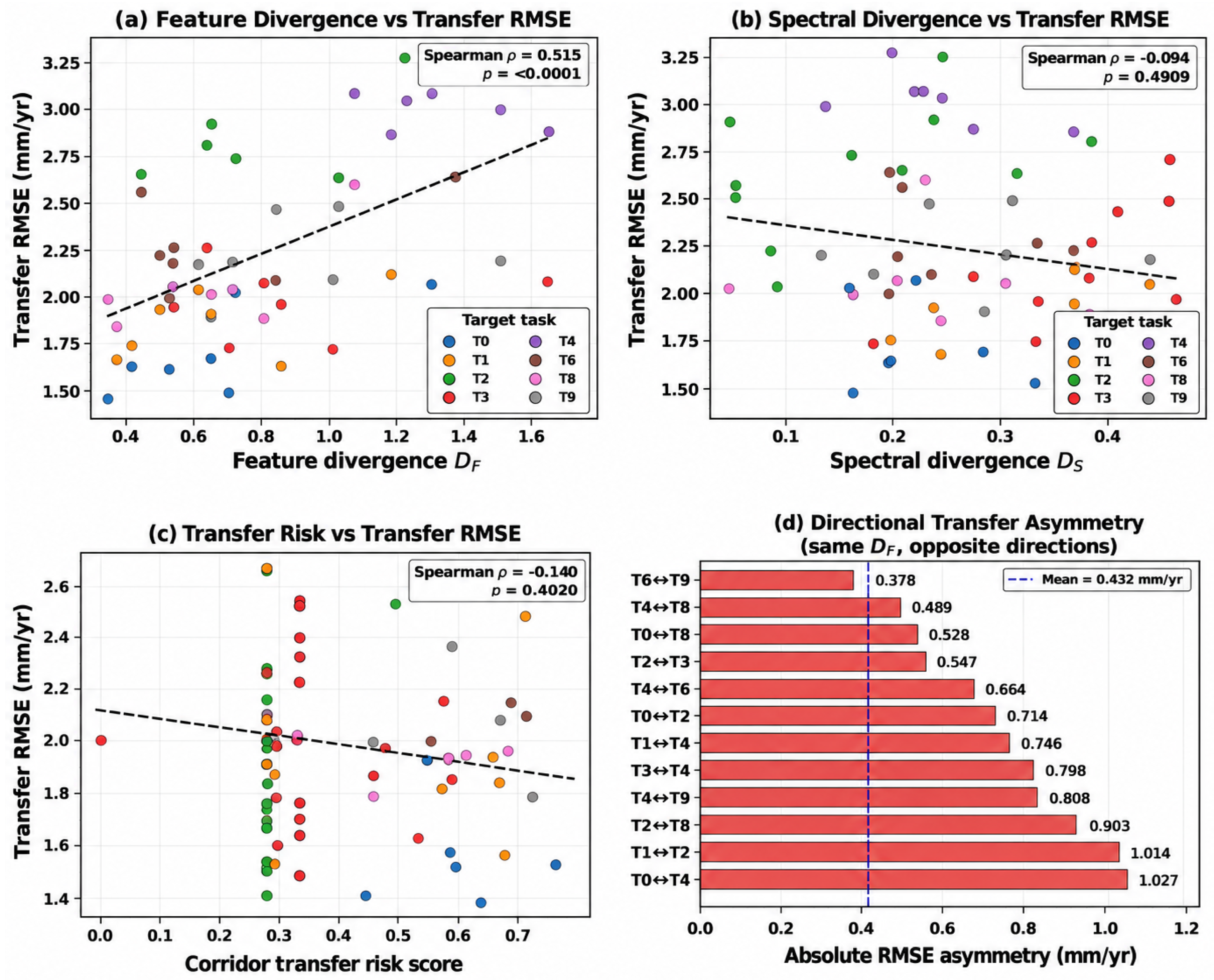
Feature–space divergence was the only transferability measure that exhibited a statistically significant relationship with transfer error. Spearman rank correlation between $D_F$ and transfer RMSE yielded $\rho =0.515$ ($p<0.001$), confirmed by Pearson $r=0.528$ ($p<0.001$), indicating that environmentally dissimilar source–target pairs consistently produce higher prediction error (Figure 7a). In contrast, spectral divergence showed no significant association with transfer RMSE ($\rho =-0.094$, $p=0.491$; Figure 7b), suggesting that graph structural similarity alone does not reliably predict transfer quality in this geotechnical context. Corridor transfer risk score was likewise non-significant ($\rho =-0.140$, $p=0.402$; Figure 7c), indicating that risk-based screening complements but does not substitute for feature–space divergence as a transferability criterion.

A pronounced directional asymmetry was observed across task pairs (Figure 7d). Despite sharing identical symmetric divergence values, transfer RMSE differed substantially depending on direction, with a mean absolute asymmetry of 0.432 mm/yr and a maximum of 1.027 mm/yr for the T0 ↔ T4 pair. Pairs involving Task 4 accounted for four of the five most asymmetric cases, consistent with the absence of eligible transfer sources identified for that domain. These findings demonstrate that symmetric divergence measures are necessary but insufficient predictors of transfer performance, and that directional factors, including source domain coverage and target task difficulty, must be incorporated into any operationally reliable transferability assessment framework.

6.7. Evidence Reliability Assessment

Evidence reliability was assessed at corridor level using three complementary indicators: EGMS point density, road coverage proxy, and observation count. Of the 140 monitored corridors, 96 (68.6%) were classified as Low evidence reliability, 28 (20.0%) as Medium, and 16 (11.4%) as High, reflecting the characteristically sparse distribution of InSAR coherent scatterers along road corridors in this study area. High-reliability corridors exhibited a mean point density of 16.568 pts/km and a mean road coverage of 54.3%, compared with 4.757 pts/km and 18.2% for Low-reliability corridors (

Table 6. Evidence reliability summary by class at corridor level. Point density and road coverage proxy are computed from EGMS observation support relative to corridor length. Validation RMSE is computed from held-out observations.

Class	Corridors	Density	Coverage	Val. RMSE	Val. MAE
		(pts/km)	(%)	(mm/yr)	(mm/yr)
High	16 (11.4%)	16.568	54.3	1.183	1.082
Medium	28 (20.0%)	13.557	45.6	1.469	1.387
Low	96 (68.6%)	4.757	18.2	1.507	1.448

).

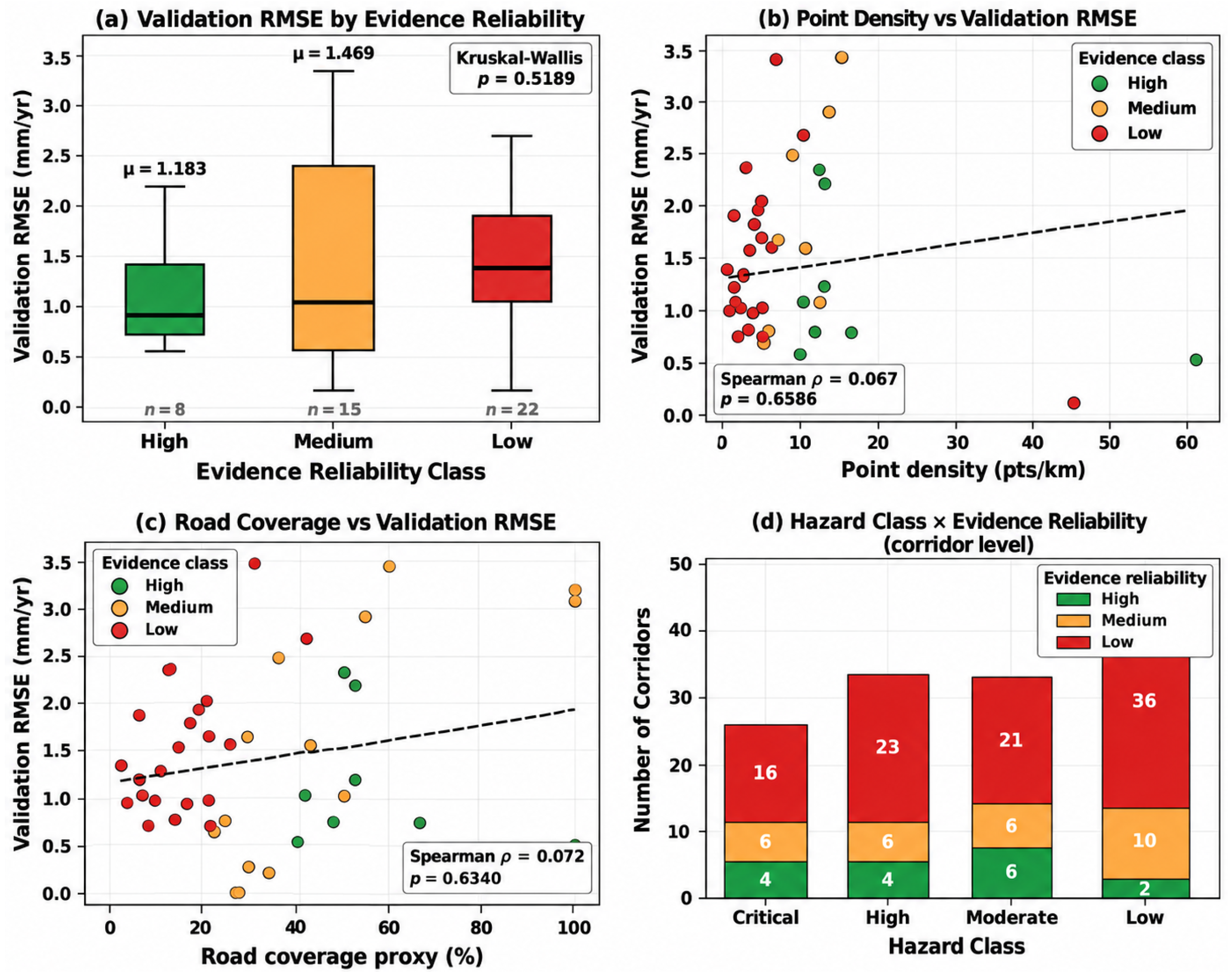
Validation against 201 held-out EGMS observations demonstrated a directionally consistent relationship between evidence reliability and prediction error (Figure 8a). High-reliability corridors achieved a mean validation RMSE of 1.183 mm/yr, compared with 1.469 mm/yr for Medium and 1.507 mm/yr for Low-reliability corridors. However, the difference was not statistically significant (Kruskal–Wallis $H=1.312$, $p=0.519$), attributable to the small number of High-reliability corridors ($n=8$) available for validation. Individual indicators of observational support, point density ($\rho =0.067$, $p=0.659$) and road coverage ($\rho =0.072$, $p=0.634$), were likewise non-significant (Figure 8b,c), suggesting that within this sparse-data regime, corridor-level evidence reliability is a necessary but not independently sufficient predictor of absolute prediction error.

The spatial distribution of evidence reliability across hazard classes (Figure 8d) reveals that Low evidence reliability predominates across all hazard levels, including 16 of 26 Critical corridors and 23 of 33 High-hazard corridors. This co-occurrence of high deformation hazard and low observational support represents the primary deployment challenge of satellite-based geotechnical monitoring and motivates the complementary role of transfer reliability introduced in the following subsection.

6.8. Transfer Reliability Assessment

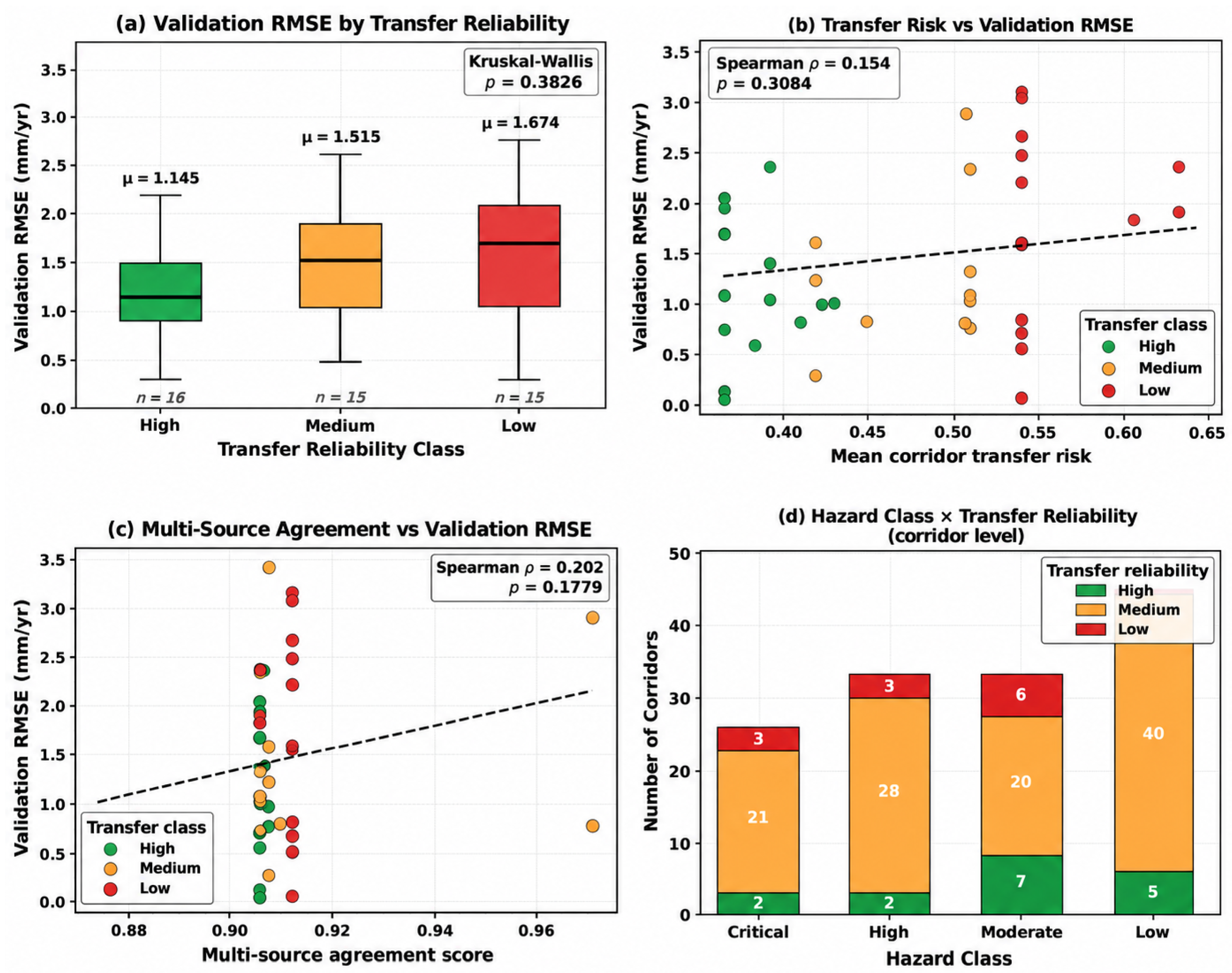
Transfer reliability was assessed at corridor level using three indicators: mean corridor transfer risk, number of eligible transfer sources, and multi-source agreement score. Of the 140 monitored corridors, 109 (77.9%) were classified as Medium transfer reliability, 16 (11.4%) as High, and 15 (10.7%) as Low (

Table 7. Transfer reliability summary by class at corridor level. Transfer risk, eligible sources, and agreement are computed from the multi-source transfer pipeline. Validation RMSE and expected error band are derived from held-out observations.

Class	N	Transfer Risk	Eligible Sources	Agreement Score	Val. RMSE (mm/yr)	Val. MAE (mm/yr)	Exp. Error (mm/yr)
High	16 (11.4%)	0.382	6.125	0.904	1.145	1.057	1.457
Medium	109 (77.9%)	0.394	4.264	0.932	1.515	1.483	1.515
Low	15 (10.7%)	0.563	4.800	0.907	1.674	1.574	1.674

). High-reliability corridors were characterised by lower mean transfer risk (0.382) and a higher mean number of eligible sources (6.125), compared with 0.563 and 4.800 for Low-reliability corridors.

Validation against held-out observations demonstrated a directionally consistent and monotonic relationship between transfer reliability class and prediction error (Figure 9a). High-reliability corridors achieved a mean validation RMSE of 1.145 mm/yr, compared with 1.515 mm/yr for Medium and 1.674 mm/yr for Low-reliability corridors, a difference of 0.529 mm/yr between the extreme classes. Transfer stability analysis corroborated this pattern: corridors in the lowest agreement quartile ($q\in (0.868,0.904$)) achieved a mean RMSE of 1.013 mm/yr, while those in the highest quartile ($q\in (0.911,0.971$)) produced 1.834 mm/yr, reflecting the adverse effect of source disagreement on prediction quality. The Kruskal–Wallis test was non-significant ($H=1.921$, $p=0.383$) owing to high within-class variance, and individual indicators, transfer risk ($\rho =0.154$, $p=0.308$), eligible sources ($\rho =-0.157$, $p=0.298$), and multi-source agreement ($\rho =0.202$, $p=0.178$), were likewise non-significant (Figure 9b,c), consistent with the small validation sample available at corridor level. To assess whether an alternative combination of the transfer-risk and source-availability components (Equation (9)) would yield a stronger association than the adopted weighting, a sensitivity sweep was conducted across the full range of relative weights. No tested combination reached statistical significance ($p>0.30$ throughout), with the adopted 0.7/0.3 weighting ($\rho =-0.109$, $p=0.470$) falling within the same non-significant range as every alternative tested, including the two single-component endpoints reported above. This confirms that the observed non-significance of transfer reliability at corridor level reflects the limited validation sample size rather than a specific, correctable weakness in the 0.7/0.3 weighting choice.

The expected prediction error band, calibrated from validation RMSE by class, ranged from 1.145 mm/yr for High-reliability corridors to 1.674 mm/yr for Low-reliability corridors. As shown in Figure 9d, Medium transfer reliability predominates across all hazard levels, including 21 of 26 Critical and 28 of 33 High-hazard corridors, underscoring that transfer knowledge is available but carries moderate uncertainty for the majority of geotechnically significant road segments in the study area.

6.9. Reliability Validation

The proposed reliability framework was validated against 201 held-out EGMS observations. Of these, 88 observations were successfully matched, within the spatial join distance threshold used for corridor-level aggregation, to 1 of the 46 road corridors comprising the validation set; the remaining 113 observations did not fall within matching distance of a validation corridor and were not included in the corridor-level reliability validation reported below. Overall prediction performance under the fused local–transfer strategy yielded an RMSE of 1.720 mm/yr and MAE of 1.353 mm/yr, outperforming both the multi-source ensemble (RMSE: 1.819 mm/yr) and sparse multi-source variant (RMSE: 1.819 mm/yr), confirming the superiority of selective single-source fusion in this geotechnical setting.

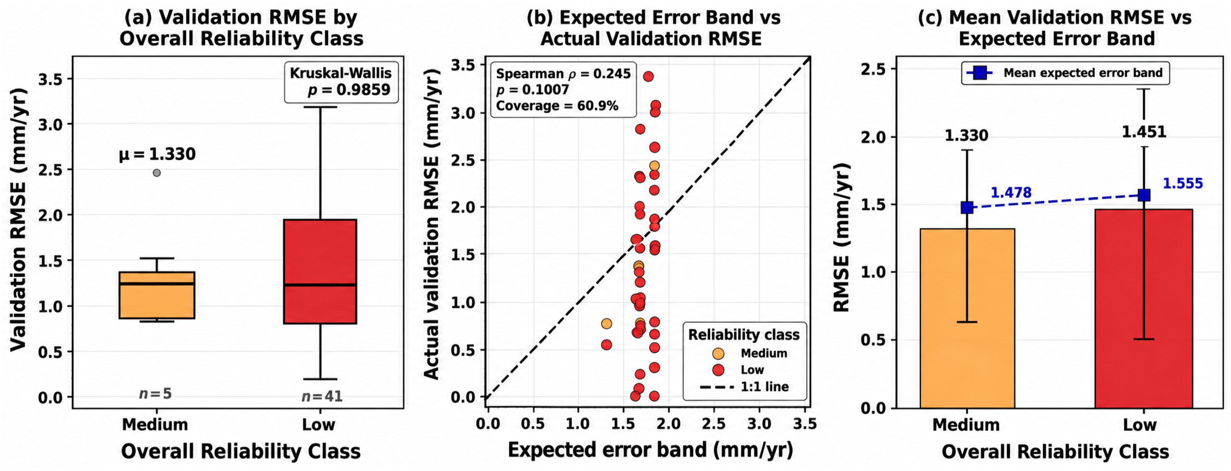
The combined overall reliability classification yielded 38 Low-reliability and 8 Medium-reliability corridors among the validation set, with no High-reliability corridors present, a distribution consistent with the characteristically sparse observational support and moderate transfer conditions identified across the study area. Medium-reliability corridors achieved a lower mean validation RMSE (1.292 mm/yr) than Low-reliability corridors (1.473 mm/yr), though the difference was not statistically significant (Kruskal–Wallis $H=0.102$, $p=0.750$; Figure 10a) owing to the small number of Medium-reliability corridors available for validation.

The expected error band, calibrated from validation RMSE by transfer and evidence reliability class, achieved an overall coverage rate of 60.9%, that is, the actual corridor RMSE fell within the predicted error band for 28 of 46 validation corridors (Figure 10b). Coverage varied by reliability class, reaching 75.0% for Medium-reliability corridors ($n=8$) and 57.9% for Low-reliability corridors ($n=38$); the lower overall coverage is therefore driven primarily by the Low-reliability class, which comprises the majority of the validation set. The Spearman correlation between expected error band and actual RMSE was positive but non-significant ($\rho =0.250$, $p=0.094$), reflecting the limited dynamic range of the error band (1.183–1.635 mm/yr) relative to the wide spread of observed RMSE values (0.016–3.388 mm/yr). The mean expected error band exceeded the mean actual RMSE (1.552 vs. 1.442 mm/yr), indicating that the framework is conservative on average, but the 60.9% empirical coverage rate indicates that this average-case conservatism does not extend uniformly to individual corridors: we therefore describe the framework’s uncertainty estimates as reliability-sensitive, with better empirical coverage for higher-reliability corridors, rather than uniformly conservatively calibrated. Validation results disaggregated by recommended action class and overall reliability are summarised in

Table 8. Reliability validation by overall reliability class. RMSE and MAE are calculated from held-out EGMS observations. Coverage is the proportion of corridors for which the observed RMSE did not exceed the expected error band.

Reliability Class	Corridors (n)	Val. Points	Mean RMSE (mm/yr)	SD RMSE (mm/yr)	Mean MAE (mm/yr)	Expected Error (mm/yr)	Coverage (%)
Medium	8	21	1.292	0.629	1.111	1.495	75.0 (6/8)
Low	38	67	1.473	0.967	1.422	1.564	57.9 (22/46)
Overall coverage							60.9 (28/46)

.

6.10. Deployment-Oriented Reliability Profiles

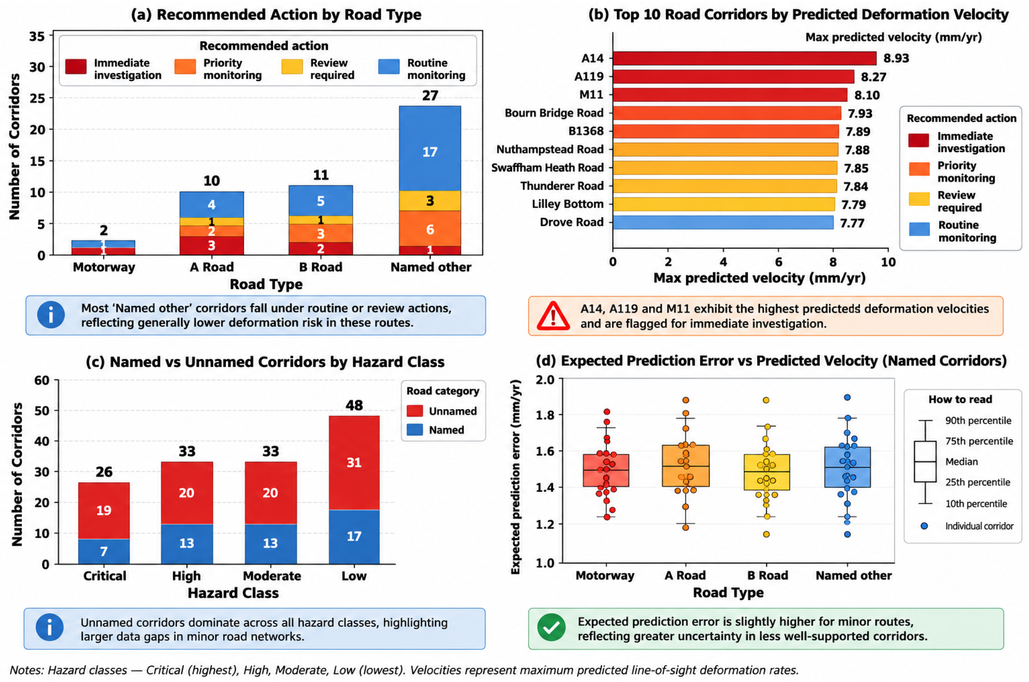
The deployment framework assigned recommended actions to all 140 monitored road corridors by integrating deformation hazard class with evidence and transfer reliability. Of the 50 named road corridors, 7 (14.0%) required immediate investigation, 11 (22.0%) priority monitoring, 5 (10.0%) review, and 27 (54.0%) routine monitoring (Figure 11a,b). Among the 90 unnamed corridors, 19 required immediate investigation and a further 19 priority monitoring, confirming that geotechnically significant deformation is not confined to the named road network (Figure 11c).

The three highest-priority named road segments were the A14 trunk road (max predicted velocity: 8.925 mm/yr; centroid: 52.301°N, 0.220°W; segment length: 2430 m), the A119 Ware Road (8.269 mm/yr; 51.805°N, 0.045°W; 510 m), and the M11 motorway (8.097 mm/yr; 52.077°N, 0.160°E; 4751 m), the only motorway in the study area flagged Critical. All three carry nationally significant traffic volumes and are located within Task 2, which exhibited the highest transfer RMSE (2.656 mm/yr) and only two eligible transfer sources, making reliable prediction particularly challenging. The A1065 Brandon Road corridor (7.316 mm/yr; 52.398°N, 0.567°E) was also flagged for immediate investigation, comprising four road segments with individual EGMS point velocities reaching −7.316 mm/yr within 106 m of the carriageway. The B1368 London Road (7.886 mm/yr; 51.992°N, 0.015°E; 534 m) and B1063 Ashley Road (7.288 mm/yr; 52.235°N, 0.447°E; 223 m) were also flagged Critical under the calibrated hazard classification (Equation (26)), representing B-road infrastructure whose predicted deformation and severity-fraction profile place them in the study area’s highest empirical hazard category, despite peak velocities below those of the highest-priority named corridors above. Named and unnamed road profiles are summarised in

Table 9. Named road corridors requiring immediate investigation or priority monitoring, ranked by maximum predicted deformation velocity. Coordinates denote the segment centroid. Ev. rel.: evidence reliability; Tr. rel.: transfer reliability; Act.: I = Immediate investigation, P = Priority monitoring, R = Review required.

Road	Type	Max Vel. (mm/yr)	Lat (°N)	Lon (°)	Length (m)	Ev. Rel.	Tr. Rel.	Act.
A14	A Road	8.925	52.301	−0.220	2430	Low	Medium	I
A119	A Road	8.269	51.805	−0.045	510	Medium	Medium	I
M11	Motorway	8.097	52.077	+0.160	4751	Low	Medium	I
B1368	B Road	7.886	51.992	+0.015	534	Low	Medium	I
A1065	A Road	7.316	52.398	+0.567	2458	Low	High	I
B1063	B Road	7.288	52.235	+0.447	223	Low	Low	I
A414	A Road	7.932	51.801	−0.044	339	Low	Medium	P
A505	A Road	7.853	—	—	—	Medium	Low	R
A6	A Road	7.684	52.147	−0.507	784	Low	Medium	P
B1382	B Road	7.140	52.415	+0.334	762	Low	Medium	P
B1104	B Road	6.845	52.410	+0.348	1149	Low	Medium	P

and

Table 10. Unnamed road segments requiring immediate investigation, ranked by maximum predicted deformation velocity. These segments lack official road designations in the OS Open Roads dataset but exhibit Critical hazard levels comparable to or exceeding those of named infrastructure. The nearest EGMS observation coordinates and predicted velocities are reported to support field identification.

Segment ID (Abbreviated)	Max Vel. (mm/yr)	EGMS Lat (°N)	EGMS Lon (°)	Ev. Rel.	Tr. Rel.	Exp. Err. (mm/yr)
UNNAMED_002674ED	8.518	52.313	−0.245	Low	Medium	1.515
UNNAMED_FB244A8F	8.429	52.093	+0.135	Low	Medium	1.515
UNNAMED_E714721E	8.342	52.168	+0.164	High	Medium	1.515
UNNAMED_B7E9537A	8.292	52.090	+0.126	High	Medium	1.515
UNNAMED_BA42F68D	8.226	51.991	−0.252	Low	Medium	1.515
UNNAMED_4E7AB428	8.214	52.089	+0.125	Low	Medium	1.515
UNNAMED_873C679D	8.214	52.089	+0.125	Low	Medium	1.515
UNNAMED_9111814B	8.214	52.089	+0.125	Low	Medium	1.515
UNNAMED_E90BEAB3	8.197	52.090	+0.041	High	Medium	1.515
UNNAMED_AABB6D0C	8.101	52.155	+0.172	High	Low	1.674
UNNAMED_4AFBFBB9	8.059	51.547	+0.510	Low	Medium	1.515
UNNAMED_95DF7D78	8.016	51.521	+0.133	Medium	Medium	1.515
UNNAMED_C2F5BF1C	7.749	52.156	+0.181	Medium	Low	1.674
UNNAMED_EB7438A1	7.210	52.323	+0.233	Low	High	1.507
UNNAMED_D572AF97	7.186	52.409	+0.542	Low	Medium	1.515
UNNAMED_2792EEF0	7.184	52.310	+0.464	Medium	Medium	1.515
UNNAMED_2053859E	7.161	52.406	+0.547	Low	Medium	1.515
UNNAMED_1624431A	7.109	52.409	+0.545	Medium	Medium	1.515
UNNAMED_79DE06C4	7.089	52.360	+0.543	Medium	Medium	1.515

respectively.

6.11. Hazard Classification Accuracy Under Prediction Compression

The compression bias quantified in Section 6.2 has direct consequences for the accuracy of the categorical hazard classification (Equation (28)) used throughout the deployment framework since this classification is derived from predicted rather than observed velocity magnitudes. To assess this effect, an observed-velocity hazard classification was constructed for the 46 validation corridors using the velocity-quantile criterion of the calibrated hazard rule (Section 6.10, Equation (28)) applied to observed rather than predicted maximum absolute velocity, and cross-tabulated against the predicted hazard classification for the same corridors. This comparison uses the velocity-quantile criterion only, omitting the corridor-level severity-fraction condition ($F_C$, $F_{HC}$) that also contributes to the full calibrated rule, since the point-level threshold underlying that fraction was not independently verified against this validation set; the confusion matrix presented in

Table 11. Confusion matrix comparing predicted and observed hazard classification for the 46 validation corridors, using the velocity-quantile criterion of the calibrated hazard rule. Rows denote the classification obtained from observed velocity; columns denote the classification obtained from predicted velocity.

Observed	Predicted
	Critical	High	Moderate	Low
Critical	0	0	3	3
High	1	2	1	2
Moderate	1	2	3	5
Low	3	3	4	13

should therefore be interpreted as an approximation of the full deployed rule’s behaviour rather than an exact reproduction of it.

Overall agreement between predicted and observed classification was 39.1% (18 of 46 corridors on the diagonal). Performance on the Critical class, the category most directly relevant to infrastructure safety decisions, was poor: of the six corridors classified as Critical by observed velocity, none were classified as Critical by predicted velocity (recall = 0%), and of the corridors classified as Critical by predicted velocity, none were true Critical corridors by observed velocity (precision = 0%). Truly Critical corridors were instead predominantly classified as Moderate or Low, consistent with the compression of predicted velocities toward the centre of their distribution reported in Section 6.2, while several truly Low-hazard corridors were classified as Critical or High, indicating that misclassification occurs in both directions rather than as a uniform downward bias alone.

7. Discussion

The results demonstrate that, within the investigated study area, reliable spatial transfer learning depends primarily on environmental similarity between source and target regions rather than on structural similarity alone. Feature–space divergence exhibited a significant positive relationship with transfer prediction error, whereas spectral divergence showed no meaningful association with transfer performance. This finding suggests that transferred knowledge remains most effective when source and target tasks share comparable environmental conditions, and that environmental compatibility should be prioritised during source selection. The observed directional asymmetry further indicates that transferability is not inherently reciprocal, highlighting the importance of considering source-task suitability and target-task complexity when designing operational transfer-learning systems.

The proposed reliability framework revealed that evidence reliability and transfer reliability capture distinct but complementary aspects of prediction confidence. Evidence reliability reflects the quantity and spatial representativeness of available observations, whereas transfer reliability reflects the expected quality of externally transferred knowledge. Neither reliability component achieved statistical significance during validation (evidence reliability: Kruskal–Wallis $H=1.312$, $p=0.519$; transfer reliability: $H=1.921$, $p=0.383$; individual indicators non-significant with p ranging from 0.178 to 0.659), and this result should be read as the primary finding regarding validation strength rather than a secondary caveat. Both components did exhibit a monotonic ordering in point estimates, whereby higher reliability classes corresponded to lower observed mean RMSE, but given the non-significance reported above and the small number of held-out corridors available at each reliability class, this ordering should be interpreted as a directionally consistent descriptive pattern rather than a statistically established relationship. We report this pattern because it may still be practically informative under the sparse observational conditions characteristic of this study, but we do not present it as evidence that reliability class reliably predicts prediction error in a statistically confirmed sense.

From an infrastructure-monitoring perspective, the deployment-oriented reliability profiles provide information that extends beyond deformation magnitude alone. The results show that many high-hazard road corridors are simultaneously characterised by low observational support, creating situations where deformation risk is high but confidence in the available evidence remains limited. By explicitly separating hazard, evidence reliability, transfer reliability, and expected error, the proposed framework enables infrastructure managers to distinguish between locations that require immediate intervention and locations that require additional monitoring or data acquisition before operational decisions are made.

Several limitations should be acknowledged. First, the study was conducted using a single EGMS tile within Eastern England, and therefore the transferability patterns identified may not fully represent other geological or climatic settings. The study is further scoped to a single deformation mechanism, characterised by gradual, subsidence-type ground motion within a predominantly flat agricultural and infrastructure landscape; the proposed framework has not been evaluated against structurally distinct deformation processes such as mining-induced subsidence, landslide movement, or coastal consolidation, each of which may involve different governing mechanisms, spatial signatures, and rates of deformation. Second, reliability validation was constrained by the relatively small number of held-out observations available at corridor level, limiting the statistical power of significance testing. Third, all validation in this study is internal to the EGMS observational record, and no independent ground-truth measurements, such as long-term GNSS or precise levelling data, were used to assess the absolute accuracy of the underlying deformation observations themselves. Independent validation against GNSS is naturally a time-series comparison problem, since continuous or campaign-based GNSS observations are inherently temporally resolved, whereas the present study uses a static mean-velocity product; meaningful alignment between the two would require the same temporal-divergence characterisation identified above as a prerequisite for spatiotemporal transfer learning. We therefore consider rigorous GNSS-based ground-truthing to be more appropriately positioned as a validation step for the spatiotemporal extension of this framework, rather than a component that can be added to the present static formulation without first resolving that same temporal alignment problem. Fourth, the transfer-learning framework relies on environmental similarity measures derived from available explanatory variables and may not capture all geotechnical processes governing deformation behaviour. Finally, the use of Random Forest models introduces substantial prediction smoothing that materially compromises categorical hazard classification accuracy: predicted velocity standard deviation was only 25–29% of observed velocity standard deviation (Section 6.2), and cross-tabulating predicted against observed hazard classification for the validation corridors showed that none of the six truly Critical-hazard corridors were correctly classified as Critical by the framework (0% recall and 0% precision on the Critical class; Section 6.11). This is a substantive limitation rather than a minor caveat: while the framework’s continuous error metrics and reliability-class validation demonstrate meaningful predictive skill on average, the categorical hazard labels used to prioritise deployment decisions should not be treated as reliable indicators of which specific corridors are most severely affected, and this limitation should be weighed directly against the framework’s practical value for infrastructure prioritisation.

Future research should evaluate the proposed framework across larger geographical regions and a wider range of deformation mechanisms, including mining subsidence, landslides, and coastal settlement processes. The incorporation of temporal EGMS observations into a joint spatiotemporal transfer-learning framework is a deliberate direction for future work rather than an oversight in the present study: such an extension requires first characterising temporal divergence between source and target monitoring tasks as an additional, independent transferability dimension, and establishing how temporal divergence interacts with the environmental divergence measure already validated in this study before the two can be combined into a single reliability-scoring framework. Investigating this joint spatiotemporal divergence structure, and only then extending the reliability framework to dynamic, time-resolved assessment, would allow reliability to be assessed dynamically and could support early-warning applications. Additional work is also needed to investigate physics-informed transfer-learning approaches that combine data-driven transferability assessment with geotechnical process knowledge. Such developments may improve both prediction accuracy and reliability estimation, thereby enhancing the practical deployment of satellite-derived deformation monitoring systems.

8. Conclusions

This study presented an evidence-based reliability assessment framework for spatial transfer learning in satellite-derived ground deformation monitoring. The framework integrates transferability-aware prediction, reliability quantification, and deployment-oriented reliability reporting within a unified monitoring workflow. The findings below were obtained within a single 100 km × 100 km EGMS tile in Eastern England, characterised by gradual, subsidence-type ground motion in a predominantly flat agricultural and infrastructure landscape, and should be interpreted within this scope rather than as general properties of spatial transfer learning across deformation mechanisms or geological settings. The principal conclusions are as follows:

1.

Environmental similarity is a meaningful predictor of transfer-learning performance in ground deformation monitoring within the investigated study area. Feature–space divergence exhibited a significant positive relationship with transfer prediction error, indicating that environmentally similar regions provide more suitable sources for knowledge transfer.

2.

Structural similarity, represented by graph spectral divergence, did not demonstrate a significant relationship with transfer prediction error. This suggests that environmental similarity is a more informative transferability indicator than spatial graph structure within the investigated study area.

3.

The local–transfer fusion approach achieved the best overall predictive performance, outperforming both full and sparse multi-source ensemble strategies. This finding indicates that selectively combining local observations with knowledge from suitable source regions is more effective than aggregating multiple transfer sources.

4.

Evidence reliability and transfer reliability both exhibited a monotonic ordering in point estimates, whereby corridors assigned higher reliability classes generally produced lower mean validation errors than corridors assigned lower reliability classes; however, this relationship did not reach statistical significance for either measure (evidence reliability: $p=0.519$; transfer reliability: $p=0.383$), constrained by the small number of held-out corridors available at each reliability class. We report this ordering as a directionally consistent descriptive pattern rather than a statistically established relationship.

5.

A substantial proportion of high-hazard road corridors were characterised by low observational support, demonstrating that deformation hazard and prediction confidence should not be interpreted as equivalent quantities.

6.

The proposed reliability framework provides additional information beyond prediction accuracy by explicitly quantifying the strength of local evidence and the trustworthiness of transferred knowledge. This enables more informed interpretation of satellite-derived deformation predictions in infrastructure monitoring applications.

References

1. Raucoules, D.; Colesanti, C.; Carnec, C. Use of SAR Interferometry for Detecting and Assessing Ground Subsidence. C. R. Geosci. 2007, 339, 289–302. [Google Scholar] [CrossRef] [Scilit]
2. Glod-Lendvai, A.M. Subsidence Determined by InSAR—A Review. Geogr. Pol. 2018, 91, 335–346. [Google Scholar] [CrossRef] [Scilit]
3. Aswathi, J.; Binojkumar, R.B.; Oommen, T.; Bouali, E.; Sajinkumar, K.S. InSAR as a Tool for Monitoring Hydropower Projects: A Review. Eng. Geol. 2022, 297, 106497. [Google Scholar] [CrossRef] [Scilit]
4. Bagheri, M. Data-Driven Prediction of Rainfall-Triggered Slope Movements Using Flume Tests and Machine Learning. Transp. Infrastruct. Geotechnol. 2025, 12, 305. [Google Scholar] [CrossRef] [Scilit]
5. Crosetto, M.; Solari, L.; Balasis-Levinsen, J.; Casagli, N.; Frei, M.; Oyen, A.; Moldestad, D.A. Ground Deformation Monitoring at Continental Scale: The European Ground Motion Service. In Proceedings of the ISPRS Archives; ISPRS: Hanover, Germany, 2020; Volume XLIII-B3-2020, pp. 293–298. [Google Scholar] [CrossRef] [Scilit]
6. Crosetto, M.; Solari, L.; Balasis-Levinsen, J.; Bateson, L.; Casagli, N.; Frei, M.; Oyen, A.; Moldestad, D.A.; Mróz, M. Deformation Monitoring at European Scale: The Copernicus Ground Motion Service. In Proceedings of the ISPRS Archives; ISPRS: Hanover, Germany, 2021; Volume XLIII-B3-2021, pp. 141–146. [Google Scholar] [CrossRef] [Scilit]
7. Costantini, M.; Minati, F.; Trillo, F.; Ferretti, A.; Passera, E.; Rucci, A.; Dehls, J.; Larsen, Y.; Marinkovic, P.; Eineder, M.; et al. EGMS: Europe-Wide Ground Motion Monitoring Based on Full Resolution InSAR Processing of All Sentinel-1 Acquisitions. In Proceedings of the IEEE International Geoscience and Remote Sensing Symposium (IGARSS); IEEE: Piscataway, NJ, USA, 2022; pp. 6980–6983. [Google Scholar] [CrossRef] [Scilit]
8. Pepe, A.; Calò, F. A Review of Interferometric Synthetic Aperture RADAR (InSAR) Multi-Track Approaches for the Retrieval of Earth’s Surface Displacements. Appl. Sci. 2017, 7, 1264. [Google Scholar] [CrossRef] [Scilit]
9. Rahmati, O.; Falah, F.; Naghibi, S.A.; Biggs, T.; Soltani, M.; Deo, R.; Cerdà, A.; Mohammadi, F.; Bui, D.T. Land Subsidence Modelling Using Tree-Based Machine Learning Algorithms. Sci. Total Environ. 2019, 672, 239–252. [Google Scholar] [CrossRef] [Scilit] [PubMed]
10. Yazbeck, J.; Rundle, J. Predicting Short-Term Deformation in the Central Valley Using Machine Learning. Remote Sens. 2023, 15, 449. [Google Scholar] [CrossRef] [Scilit]
11. Guo, Y.; Hu, S.; Wu, W.; Wang, Y.; Senthilnath, J. Multitemporal Time Series Analysis Using Machine Learning Models for Ground Deformation in the Erhai Region, China. Environ. Monit. Assess. 2020, 192, 487. [Google Scholar] [CrossRef] [Scilit] [PubMed]
12. Yang, J.; Kou, P.; Dong, X.; Xia, Y.; Gu, Q.; Tao, Y.; Feng, J.; Ji, Q.; Wang, W.; Avtar, R. Reservoir Water Level Decline Accelerates Ground Subsidence: InSAR Monitoring and Machine Learning Prediction of Surface Deformation in the Three Gorges Reservoir Area. Front. Earth Sci. 2024, 12, 1503634. [Google Scholar] [CrossRef] [Scilit]
13. Bagheri, M.; Tshireletso, T.; Ghorashi, S.A. From Multisensor Fusion to Intelligent Geospatial Monitoring: Emerging Architectures for Geotechnical Hazard Assessment. Remote Sens. 2026, 18, 2669. [Google Scholar] [CrossRef] [Scilit]
14. Ma, Y.; Chen, S.; Ermon, S.; Lobell, D.B. Transfer learning in environmental remote sensing. Remote Sens. Environ. 2024, 301, 113924. [Google Scholar] [CrossRef] [Scilit]
15. Nowakowski, A.; Del Rosso, M.P.; Zachar, P.; Spiller, D.; Gabara, G.; Barretta, D.; Kalinowska, K.B.; Choromański, K.; Wilkowski, A.; Sebastianelli, A.; et al. Transfer Learning in Earth Observation Data Analysis: A Review. IEEE Geosci. Remote Sens. Mag. 2025, 13, 121–152. [Google Scholar] [CrossRef] [Scilit]
16. Murakami, D.; Kajita, M.; Kajita, S. Spatial process-based transfer learning for prediction problems. J. Geogr. Syst. 2025, 27, 147–166. [Google Scholar] [CrossRef] [Scilit]
17. Ludwig, M.; Moreno-Martínez, A.; Hölzel, N.; Pebesma, E.; Meyer, H. Assessing and improving the transferability of current global spatial prediction models. Glob. Ecol. Biogeogr. 2023, 32, 356–368. [Google Scholar] [CrossRef] [Scilit]
18. Tyralis, H.; Papacharalampous, G. A Review of Predictive Uncertainty Estimation with Machine Learning. Artif. Intell. Rev. 2024, 57, 94. [Google Scholar] [CrossRef] [Scilit]
19. Singh, G.; Moncrieff, G.; Venter, Z.; Cawse-Nicholson, K.; Slingsby, J.; Robinson, T.B. Uncertainty Quantification for Probabilistic Machine Learning in Earth Observation Using Conformal Prediction. Sci. Rep. 2024, 14, 16166. [Google Scholar] [CrossRef] [Scilit] [PubMed]
20. Lou, X.; Luo, P.; Meng, L. GeoConformal Prediction: A Model-Agnostic Framework for Measuring the Uncertainty of Spatial Prediction. Ann. Am. Assoc. Geogr. 2025, 115, 1971–1998. [Google Scholar] [CrossRef] [Scilit]
21. Prati, C.; Ferretti, A.; Perissin, D. Recent Advances on Surface Ground Deformation Measurement by Means of Repeated Space-Borne SAR Observations. Remote Sens. Environ. 2010, 114, 2037–2055. [Google Scholar] [CrossRef] [Scilit]
22. Bianchini, S.; Raspini, F.; Solari, L.; Del Soldato, M.; Ciampalini, A.; Rosi, A.; Casagli, N. From Picture to Movie: Twenty Years of Ground Deformation Recording Over Tuscany Region (Italy) With Satellite InSAR. Front. Earth Sci. 2018, 6, 177. [Google Scholar] [CrossRef] [Scilit]
23. Festa, D.; Casagli, N.; Casu, F.; Confuorto, P.; De Luca, C.; Del Soldato, M.; Lanari, R.; Manunta, M.; Manzo, M.; Raspini, F. Automated Classification of A-DInSAR-Based Ground Deformation by Using Random Forest. GISci. Remote Sens. 2023, 60, 2134561. [Google Scholar] [CrossRef] [Scilit]
24. Huynh, N.; Nguyen, G.T.; Ha, T.; Le, D.; Tran, V.A. Machine Learning Approaches for Predicting Land Subsidence in Ca Mau: XGBoost, Random Forest, and MAF. Inz. Miner. 2025, 1, 703–714. [Google Scholar] [CrossRef] [Scilit]
25. Yaragunda, V.R.; Vaka, D.S.; Oikonomou, E. Land Subsidence Susceptibility Modelling in Attica, Greece: A Machine Learning Approach Using InSAR and Geospatial Data. Earth 2025, 6, 61. [Google Scholar] [CrossRef] [Scilit]
26. Xu, Y.; Zhao, Y.; Jiang, Q.; Sun, J.; Tian, C.; Jiang, W. Machine-Learning-Based Deformation Prediction Method for Deep Foundation-Pit Enclosure Structure. Appl. Sci. 2024, 14, 1273. [Google Scholar] [CrossRef] [Scilit]
27. Wang, X.; Qin, Z.; Bai, X.; Hao, Z.; Yan, N.; Han, J. Research Progress of Machine Learning in Deep Foundation Pit Deformation Prediction. Buildings 2025, 15, 852. [Google Scholar] [CrossRef] [Scilit]
28. Harle, S.; Wankhade, R. Machine Learning Techniques for Predictive Modelling in Geotechnical Engineering: A Succinct Review. Discov. Civ. Eng. 2025, 2, 86. [Google Scholar] [CrossRef] [Scilit]
29. Iddianozie, C.; McArdle, G. A Transfer Learning Paradigm for Spatial Networks. In Proceedings of the 2nd ACM SIGSPATIAL International Workshop on AI for Geographic Knowledge Discovery, Seattle, WA, USA, 5 November 2019. [Google Scholar] [CrossRef] [Scilit]
30. Hoffimann, J.; Zortea, M.; Carvalho, B.d.; Zadrozny, B. Geostatistical Learning: Challenges and Opportunities. Front. Appl. Math. Stat. 2021, 7, 689393. [Google Scholar] [CrossRef] [Scilit]
31. Paul, A.; Rottensteiner, F.; Heipke, C. Transfer Learning Based on Logistic Regression. In Proceedings of the ISPRS Archives; ISPRS: Hanover, Germany, 2015; Volume XL-3/W3, pp. 145–149. [Google Scholar] [CrossRef] [Scilit]
32. Yaghmour, A.; Prasad, S.; Crawford, M.M. Attention Guided Semisupervised Generative Transfer Learning for Hyperspectral Image Analysis. IEEE J. Sel. Top. Appl. Earth Obs. Remote Sens. 2024, 17, 19884–19900. [Google Scholar] [CrossRef] [Scilit]
33. Siddique, T.; Mahmud, M.S.; Keesee, A.M.; Ngwira, C.M.; Connor, H. A Survey of Uncertainty Quantification in Machine Learning for Space Weather Prediction. Geosciences 2022, 12, 27. [Google Scholar] [CrossRef] [Scilit]
34. Malarvizhi, A.S.; Smith, K.; Yang, C. Uncertainty Quantification in Geospatial AI/ML Applications: Methods, Metrics, and Open-Source Support with an Air Quality Use Case. Big Earth Data 2026, 1–34. [Google Scholar] [CrossRef] [Scilit]
35. Papacharalampous, G.; Tyralis, H.; Doulamis, N.; Doulamis, A. Uncertainty Estimation of Machine Learning Spatial Precipitation Predictions from Satellite Data. Mach. Learn. Sci. Technol. 2024, 5, 035044. [Google Scholar] [CrossRef] [Scilit]
36. Kakhani, N.; Alamdar, S.; Kebonye, N.M.; Amani, M.; Scholten, T. Uncertainty Quantification of Soil Organic Carbon Estimation from Remote Sensing Data with Conformal Prediction. Remote Sens. 2024, 16, 438. [Google Scholar] [CrossRef] [Scilit]
37. Lou, X.; Luo, P.; Li, Z.; Gao, S.; Meng, L. GeoXCP: Uncertainty Quantification of Spatial Explanations in Explainable AI. Int. J. Geogr. Inf. Sci. 2026, 40, 2753–2783. [Google Scholar] [CrossRef] [Scilit]
38. Coulston, J.W.; Blinn, C.E.; Thomas, V.A.; Wynne, R.H. Approximating Prediction Uncertainty for Random Forest Regression Models. Photogramm. Eng. Remote Sens. 2016, 82, 189–197. [Google Scholar] [CrossRef] [Scilit]
39. MacQueen, J. Some Methods for Classification and Analysis of Multivariate Observations. In Proceedings of the Fifth Berkeley Symposium on Mathematical Statistics and Probability; University of California Press: Berkeley, CA, USA, 1967; Volume 1, pp. 281–297. [Google Scholar]
40. Hubert, L.; Arabie, P. Comparing Partitions. J. Classif. 1985, 2, 193–218. [Google Scholar] [CrossRef] [Scilit]
41. Rubner, Y.; Tomasi, C.; Guibas, L.J. The Earth Mover’s Distance as a Metric for Image Retrieval. Int. J. Comput. Vis. 2000, 40, 99–121. [Google Scholar] [CrossRef] [Scilit]
42. Chung, F.R.K. Spectral Graph Theory; CBMS Regional Conference Series in Mathematics; American Mathematical Society: Providence, RI, USA, 1997; Volume 92. [Google Scholar]
43. Breiman, L. Random Forests. Mach. Learn. 2001, 45, 5–32. [Google Scholar] [CrossRef] [Scilit]
Figure 1. Study area, EGMS vertical deformation observations, and road-network monitoring domains. The inset shows the location of the 100 × 100 km study tile within England. The main panel shows the eight spatial monitoring task domains (T0–T9, excluding T5 and T7) used for spatial transfer learning, overlaid with EGMS mean vertical deformation velocity observations (2019–2023, coloured by velocity) and major road infrastructure coloured by deformation hazard class. Selected nationally significant road corridors (M11, A14, A1065, A119, and B1368) are labelled directly on the map.
Remotesensing 18 03136 g001
Figure 2. Overview of the proposed transferability-aware monitoring framework. The framework consists of three stages: (i) transferability-aware monitoring for generating deformation predictions, (ii) evidence-based reliability assessment for quantifying prediction trustworthiness, and (iii) validation for evaluating predictive performance and reliability behaviour.
Remotesensing 18 03136 g002
Figure 3. Conceptual spatial task construction based on clustering of geographic and environmental attributes. Each colour represents one spatial monitoring task used as a source or target domain within the spatial transfer learning framework. The partition was obtained using stability-selected K-means clustering in a standardised spatial–environmental feature space comprising geographic coordinates, elevation, distance to water bodies, and distance to urban areas.
Remotesensing 18 03136 g003
Figure 4. Conceptual representation of the proposed reliability framework. Evidence reliability and transfer reliability are evaluated independently and subsequently reported together as complementary indicators of prediction confidence.
Remotesensing 18 03136 g004
Figure 5. Deployment-oriented reliability decomposition. Each deformation prediction is accompanied by a reliability profile consisting of predicted hazard, evidence reliability, transfer reliability, and validation-calibrated expected prediction error. Together, these components provide interpretable information for infrastructure monitoring and decision support.
Remotesensing 18 03136 g005
Figure 6. Cross-task transfer performance. (a) RMSE by target task for the fused baseline, multi-source ensemble, and sparse multi-source ensemble. (b) Directional transfer RMSE matrix (source × target). (c) Observed versus predicted deformation velocities under the multi-source strategy. (d) MAE by target task across prediction strategies.
Remotesensing 18 03136 g006
Figure 7. Relationship between transferability measures and transfer prediction error. (a) Feature–space divergence D F versus transfer RMSE ( ρ = 0.515 , p < 0.001 ). (b) Spectral divergence D S versus transfer RMSE (non-significant). (c) Corridor transfer risk score versus transfer RMSE (non-significant). (d) Directional RMSE asymmetry for the twelve most asymmetric task pairs sharing identical D F ; dashed line denotes the mean asymmetry of 0.432 mm/yr.
Remotesensing 18 03136 g007
Figure 8. Evidence reliability assessment. (a) Validation RMSE distribution by evidence reliability class (Kruskal–Wallis p = 0.519 ). (b) Point density versus validation RMSE ( ρ = 0.067 , p = 0.659 ). (c) Road coverage proxy versus validation RMSE ( ρ = 0.072 , p = 0.634 ). (d) Distribution of evidence reliability classes across deformation hazard levels at corridor level.
Remotesensing 18 03136 g008
Figure 9. Transfer reliability assessment. (a) Validation RMSE distribution by transfer reliability class (Kruskal–Wallis p = 0.383 ). (b) Mean corridor transfer risk versus validation RMSE ( ρ = 0.154 , p = 0.308 ). (c) Multi-source agreement score versus validation RMSE ( ρ = 0.202 , p = 0.178 ). (d) Distribution of transfer reliability classes across deformation hazard levels at corridor level.
Remotesensing 18 03136 g009
Figure 10. Reliability validation results. (a) Validation RMSE distribution by overall reliability class. (b) Expected error band versus actual validation RMSE for all 46 corridors; points above the 1:1 line indicate under-coverage. (c) Mean validation RMSE and mean expected error band by overall reliability class, with error bars denoting one standard deviation.
Remotesensing 18 03136 g010
Figure 11. Deployment-oriented reliability profiles for named and unnamed road corridors. (a) Recommended action distribution by named road type. (b) Top 10 named road corridors ranked by maximum predicted deformation velocity, coloured by recommended action. (c) Distribution of named versus unnamed corridors across hazard classes. (d) Deformation velocity versus expected prediction error for all named road corridors, coloured by road type; annotated corridors represent geotechnically significant infrastructure.
Remotesensing 18 03136 g011