Article

Weighted Strong Product Graph Laplacian Regularization for Hyperspectral Image Mixed-Noise Removal with Superpixel Segmentation


1
School of Information and Communication, Guilin University of Electronic Technology, Guilin 541004, China
2
Guangxi Key Laboratory of Precision Navigation Technology and Application, Guilin University of Electronic Technology, Guilin 541004, China
3
School of Aerospace, Harbin Institute of Technology, Shenzhen 518055, China
*
Author to whom correspondence should be addressed.
Remote Sens. 2026, 18(18), 3162; https://doi.org/10.3390/rs18183162
Submission received: 8 July 2026 / Revised: 7 September 2026 / Accepted: 10 September 2026 / Published: 15 September 2026

Highlights

What are the main findings?
  • The Kronecker product graph used by prior superpixel/band-segmented HSI denoisers omits the pure-spatial and pure-spectral edges; restoring them through a weighted strong product graph improves Mean Peak Signal-to-Noise Ratio (MPSNR) and Erreur Relative Globale Adimensionnelle de Synthèse (ERGAS) in all 12 simulated dataset–case settings—by up to 2.5 dB in MPSNR from the graph term alone.
  • The product-graph edge type governs a spatial–spectral fidelity trade-off: pure edges drive spatial reconstruction while joint edges favour spectral fidelity (Spectral Angle Mapper, SAM), and the trade-off is tunable by a single weight β.
What are the implications of the main findings?
  • For this model family, Cartesian/strong-type products retain the pure spatial and spectral edges that the Kronecker product alone omits.
  • The low-rank block of the framework is modular (matrix or Tucker), allowing the prior to be matched to scene structure.

Abstract

Hyperspectral images (HSIs) are inevitably degraded by mixed noise, which hampers downstream interpretation. Recent graph-signal-processing denoisers encode the spatial–spectral structure of an HSI through a product graph over superpixel bodies, yet the adopted Kronecker (tensor) product graph retains only the joint spatial–spectral edges and discards the pure-spatial and pure-spectral edges—the two priors that govern HSI smoothness. We introduce a two-parameter weighted product-graph family that contains the Kronecker, Cartesian and strong products as exact special cases, and propose Weighted Strong Product Graph Laplacian Regularization (WSPGLR)—the strong-product branch with a tunable joint-edge weight β—embedded in a global low-rank plus sparse model solved by the Alternating Direction Method of Multipliers (ADMM) with singular-value-thresholding and soft-thresholding updates and a sparse conjugate-gradient (CG) solve. On three simulated cubes (Washington DC Mall, Pavia University, Indian Pines) under four mixed-noise scenarios, WSPGLR consistently improves Mean Peak Signal-to-Noise Ratio (MPSNR) and ERGAS (Erreur Relative Globale Adimensionnelle de Synthèse) over a matched Kronecker-product control in every tested case (and Mean Structural Similarity (MSSIM) in 11 of 12 settings)—up to 2.5 dB in MPSNR from the graph term alone—and an ablation shows that β governs a spatial–spectral fidelity trade-off (Spectral Angle Mapper, SAM). On the detailed urban scenes, WSPGLR attains the highest MPSNR against the external methods and matched control in seven of eight settings, whereas it trails LRTDTV on the smooth agricultural scene; with an optional scene-adaptive TV step it attains the best average rank across scene types; a Tucker-based variant further shows the low-rank block is modular and generally improves spectral fidelity. Tests on four no-reference real HSIs and 30 paired real-noise MEHSI samples extend the sensor coverage; on MEHSI, the native-domain RND framework remains substantially stronger, which delimits the scope of the proposed training-free regularizer.

1. Introduction

Hyperspectral images (HSIs) record hundreds of contiguous narrow spectral bands for every spatial location, providing rich spectral signatures that underpin mineral exploration, precision agriculture, environmental monitoring, land-cover mapping and reconnaissance [1,2]. Because the incoming radiance is divided among many narrow bands, the photon count per band is low, so sensor noise is in part signal-dependent (Poissonian shot noise superposed on a signal-independent Gaussian read/dark-current floor, with both terms varying by band and by sensor) [3], and acquired HSIs are further affected by dark current, calibration errors and push-broom scanning artifacts. The result is a mixture of noise types—zero-mean Gaussian noise, impulse (salt-and-pepper) noise, stripes and dead lines—whose statistics moreover vary from band to band [4,5]. Following common practice in the compared low-rank/graph literature, our simulated benchmark (Section 4.1) approximates this mixture with band-varying additive Gaussian and impulse noise; Section 4.6 additionally reports a physically motivated signal-dependent (Poisson–Gaussian) regime and a lower-severity case to test whether the graph-control margin persists beyond the main noise model and severity range. Removing this mixed noise without destroying the fine spatial structure and the spectral signatures is a prerequisite for reliable downstream analysis.
Three decades of research on HSI denoising can be read as a search for the right prior. Early approaches applied mature two-dimensional filters band by band—for example, the collaborative transform-domain filter BM3D [6]—but band-wise processing ignores the strong correlation among bands; volumetric extensions such as BM4D [7] treat the cube as a whole yet remain agnostic to the specific spatial–spectral anisotropy of HSIs. A second line exploits the fact that clean spectra lie near a low-dimensional subspace: low-rank tensor approximation (LRTA) [8] and PARAFAC decomposition [9] impose multilinear low-rankness, while low-rank matrix recovery (LRMR) [4] casts mixed-noise removal as robust principal component analysis on the unfolded cube and NAILRMA [5] iteratively refines a noise-adjusted low-rank approximation to accommodate band-dependent noise levels. Because low-rankness alone leaves residual spatial noise, a third line couples it with total variation (TV): LRTV [10] combines low-rank matrix factorization with spatial TV, spatio-spectral TV (SSTV) regularizes the spectral gradient as well [11], LRTDTV embeds an anisotropic SSTV in a Tucker decomposition [12], LLRGTV balances local low-rank patches against a global SSTV [13], and a recast total-variation formulation unifies the two terms [14]. A fourth line denoises the coefficients of a learned spectral subspace—FastHyDe [15] filters eigen-images non-locally, GLF adds global-and-non-local low-rank factorizations [16], NGmeet iterates between the subspace and non-local patch estimation [17], and TSLRLN lifts the construction to tensor subspaces [18]. Finally, deep networks learn spatial–spectral priors from data: HSID-CNN [19], HSI-DeNet [20] and QRNN3D [21] employ convolutional and recurrent architectures, while more recent work uses spectral-enhanced transformers [22] and self-supervised denoising diffusion models that operate on the degraded image alone [23]. Deep models are strong when training and test distributions match, but they require external training data (or costly per-image optimization) and their behavior on unseen sensors or noise mixtures is harder to control than that of model-based schemes; see [24] for a recent systematic review of the model-based (low-rank tensor) line.
A more recent, structurally different line models the HSI with tools from graph signal processing (GSP) [25,26,27]: pixels (or superpixels) are graph nodes, affinities are edges, and the graph Laplacian regularizer (GLR) x L x penalizes signal variation across connected nodes, which naturally accommodates the irregular regions produced by superpixel segmentation [28,29,30]. For multi-way data, product graphs offer a principled and scalable way to compose a graph per dimension into a joint model [31,32]: Kronecker products model recursive network structure [33], Cartesian product factors can be learned from multi-domain data [34], and graph products underpin spatio-temporal feature learning [35]. In HSI denoising specifically, the research group behind the present line of work introduced an adaptive-weight graph TV coupled with low-rank recovery [36], a large-scale distributed superpixel-based GSP restoration framework [37], then KGLRSSBS, which combines superpixel segmentation, band segmentation and a Kronecker product graph over superpixel bodies [38], and most recently LRTDKGLR, which couples the same Kronecker product-graph regularizer with a Tucker tensor decomposition [39]. A particularly relevant 2026 development is PCC-GLR [40], which constructs global and local spectral graphs from Pearson correlations and combines them with low-rank and sparse-noise terms. Notably, the strong product graph itself has been used by the same group for time-varying graph-signal inpainting [41], but it has not been explored as a spatial–spectral regularizer for HSI denoising.
Motivation. While the Kronecker product elegantly couples the two dimensions, it is too restrictive. In G c G p , two nodes ( u 1 , v 1 ) and ( u 2 , v 2 ) are adjacent only if u 1 u 2 and v 1 v 2 ; only “neighboring-pixel-and-neighboring-band” edges survive. Consequently the Kronecker graph carries neither (i) pure-spatial edges—neighboring pixels within the same band ( u 1 u 2 , v 1 = v 2 ), the dominant spatial-smoothness prior—nor (ii) pure-spectral edges—the same pixel across adjacent bands ( u 1 = u 2 , v 1 v 2 ), the most characteristic HSI prior. Both are discarded exactly where HSI signals are smoothest, and the tensor product of two connected graphs is frequently disconnected, weakening diffusion of the regularizer. Our experiments confirm that the Kronecker graph is the weakest of the canonical product graphs on the spatial-reconstruction metrics (Section 4.5).
Contribution. We argue that the strong product graph G c G p , whose edge set is the union of the Cartesian and tensor products [31], is the natural remedy: it reinstates the pure-spatial and pure-spectral edges while keeping the joint edges. To study the two edge groups systematically we cast them in a two-parameter weighted product family A α , β (Section 3.3), in which the pure edges carry a weight α and the joint edges a weight β ; the Kronecker ( α , β ) = ( 0 , 1 ) , Cartesian ( 1 , 0 ) and strong ( 1 , 1 ) products are exact special cases. The proposed WSPGLR keeps the pure edges ( α = 1 ) and tunes the single joint-edge weight β , thereby spanning the Cartesian and strong products. Our contributions are:
1.
We introduce WSPGLR, a weighted strong-product graph Laplacian regularizer for HSI denoising, built on a two-parameter product family that contains the Kronecker, Cartesian and strong products as exact special cases, with a closed-form (normalized) Laplacian.
2.
We embed WSPGLR in a global low-rank plus sparse model whose spatial graph is assembled per superpixel to preserve boundaries, and derive an ADMM solver whose graph subproblem is a sparse linear system solved iteratively by conjugate gradients.
3.
Through an ablation over Kronecker/Cartesian/strong/weighted products and comparisons on simulated and real HSIs, we show that restoring the pure spatial–spectral edges yields consistent gains over the matched Kronecker baseline, and we benchmark the resulting method against representative model-based and learned denoisers.
4.
We demonstrate that the low-rank block is modular via a Tucker tensor variant (WSPGLR-T) that improves spectral fidelity in nearly all settings, and use it for a controlled comparison isolating “graph smoother versus spatial–spectral TV” under an identical tensor prior.

2. Related Work

Low-rank matrix and tensor models. The observation that clean spectra occupy a low-dimensional subspace motivates low-rank restoration. On the matrix side, LRMR performs patch-wise robust PCA on the unfolded cube [4]; NAILRMA adapts the approximation iteratively to band-dependent noise [5]; LRTV augments low-rank factorization with spatial TV [10]. On the tensor side, LRTA applies Tucker-based multilinear approximation [8], PARAFAC imposes a canonical polyadic structure [9], LRTDTV couples Tucker low-rankness with anisotropic spatio-spectral TV [12], and LLRGTV combines local low-rank patches with a global SSTV [13]; SSTV itself regularizes spatial and spectral gradients jointly [11], and recast formulations unify low-rank and TV terms in a single functional [14]. These priors are strong for Gaussian and sparse noise but tend to over-smooth textures, and their regularizers act on regular grids rather than on the irregular regions present in natural scenes.
Subspace and non-local methods. BM4D extends non-local collaborative filtering to volumetric data [7]. Subspace methods first estimate a spectral basis and then denoise the low-dimensional eigen-images: FastHyDe exploits their high spatial correlation [15], GLF combines global and non-local low-rank factorizations [16], NGmeet alternates between subspace estimation and non-local patch denoising [17], and TSLRLN performs the construction in a tensor subspace with a non-local prior [18]. Such methods achieve high spectral fidelity but depend on accurate subspace and noise estimation, and their piecewise-smooth assumptions favour homogeneous scenes.
Deep-learning methods. HSID-CNN learns a spatial–spectral residual mapping [19], HSI-DeNet learns multi-channel filter banks for restoration [20], and QRNN3D introduces 3-D quasi-recurrent units that propagate information along the spectral dimension [21]. More recently, state-space (Mamba) architectures have been applied to HSI denoising: SSUMamba scans the cube along six spatial–spectral orders with a bidirectional selective state-space model [42], and hybrid transformer–diffusion designs such as S2TDM combine spatial–spectral self-attention with a diffusion prior for the same task [43]. Deep models attain excellent accuracy within their training distribution, at the cost of external training data, limited interpretability, and uncertain generalization to unseen sensors and noise mixtures—which keeps interpretable model-based approaches, including the present one, practically relevant. The empirical comparison includes HSDT [44], a 2023 spectral-attention transformer evaluated with its openly downloadable checkpoint. Its guided spectral self-attention module is run in the released flex mode, a band-count-agnostic dot-product formulation that accepts our 103–224-band cubes without changing checkpoint weights. QRNN3D [21], a 2021 quasi-recurrent 3-D network, is evaluated with its released complex-noise checkpoint; its fully convolutional architecture is band-count-agnostic and requires no inference adaptation. Section 4.2 reports the resulting full comparison against both and against two distinct 2025 models: the multi-prompt transformer MP-HSIR and the transformer–diffusion model S2TDM. The same benchmark also includes PCC-GLR, the 2026 model-driven Pearson spectral-graph method most closely related to our graph regularization setting. To complement their out-of-domain evaluation, Section 4.8 also compares against RND [45], a 2026 real-noise-decoupling framework, on the official held-out test split of its native MEHSI evaluation domain.
Graph and product-graph methods. GSP provides the notion of signal smoothness on irregular domains [25,26], with applications from geometric data [27] to large multi-domain data via product graphs [32]. The algebra of graph products—Cartesian, tensor (Kronecker) and strong—is classical [31]; Kronecker products model recursive real-world networks [33], Cartesian factors can be learned from data [34], and graph products support spatio-temporal representation learning [35]. For HSI denoising, superpixel segmentation supplies edge-preserving regions [28,29,30], and graph-driven TV regularizers built on spatial graphs improve over grid-based SSTV [46]; graph TV combined with low-rank priors has also proven effective beyond denoising, e.g., in heterogeneous change detection [47]. The group behind KGLRSSBS first coupled adaptive-weight graph TV with low-rank recovery [36], scaled superpixel-based GSP restoration to large scenes with a distributed algorithm [37], then introduced the superpixel-body Kronecker product graph [38], and recently combined it with a Tucker decomposition in LRTDKGLR [39]; the strong product has appeared in the group’s work on time-varying graph-signal inpainting [41], though not as an HSI regularizer. Both KGLRSSBS and LRTDKGLR adopt the Kronecker product—which we show is edge deficient—whereas our work replaces it with a weighted product family that restores the pure spatial and spectral edges, couples the graph term with a global (matrix or Tucker, Section 3.8) low-rank prior, and quantifies the edge-type trade-off through an explicit ablation. Unlike generic product-graph learning [34,35], our contribution is the specific weighted-product-graph construction for HSI mixed-noise removal and its ADMM solver with thresholding steps and a sparse CG subproblem.

3. Method

Figure 1 gives an overview of the proposed method: a superpixel-adapted spatial graph and a band path graph are combined through the weighted product-graph family into the WSPGLR regularizer, which is coupled with a global low-rank plus sparse model and solved by ADMM.

3.1. Observation Model and Notation

A graph G = ( V , E ) has (weighted) adjacency A , degree D = diag ( A 1 ) and combinatorial Laplacian L = D A ; its symmetric normalized form is L sym = I D 1 / 2 A D 1 / 2 . An observed HSI O R M × N × p (p bands) with mixed noise is modelled as
O = X + S + N ,
where X is the clean image, S collects sparse noise (impulse, stripes, dead lines) and N is Gaussian noise. We write O R M N × p for the band-wise unfolding. In the optimization, the dense perturbation is not assigned a separate variable: the low-rank and graph penalties suppress it in the estimate X , whereas S explicitly captures sparse outliers.

3.2. Superpixel Spatial Graph and Band Path Graph

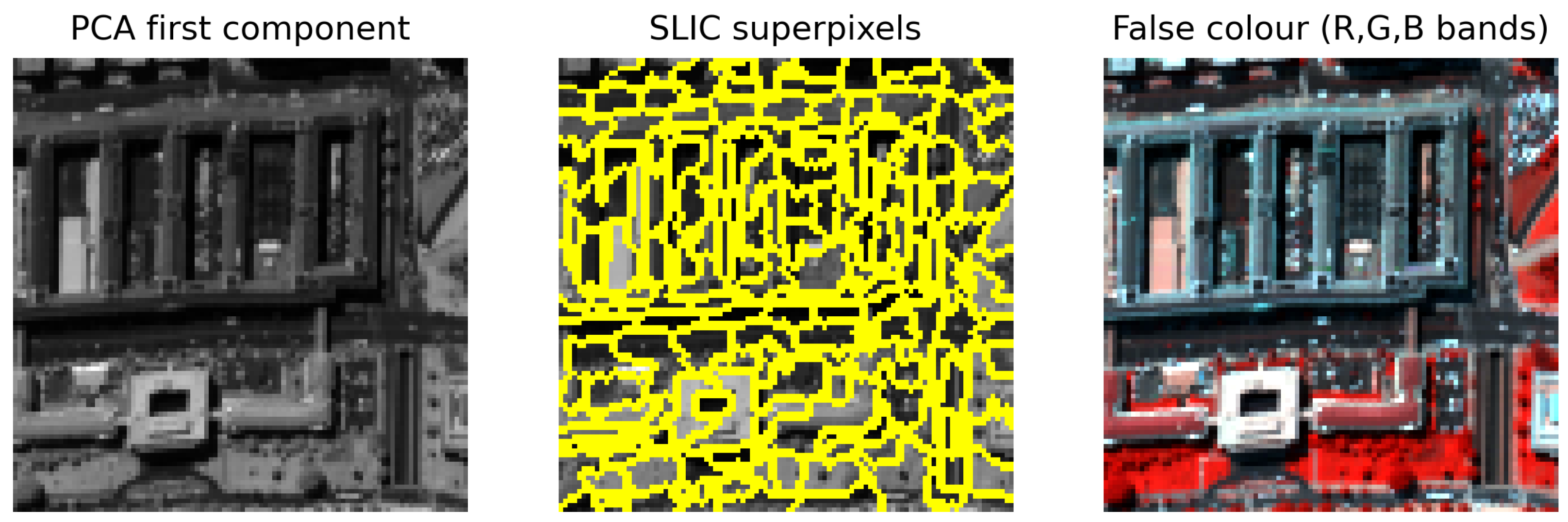
The first principal component of O is over-segmented by SLIC [28] into superpixels (Figure 2). The spatial graph G c has one node per pixel and a 4-neighbor edge between spatially adjacent pixels. Edges within a superpixel receive unit weight, while the sparse edges that cross a superpixel boundary are down-weighted by a factor w b ( w b = 0.2 throughout; w b = 0 recovers a hard cut), which preserves object boundaries without introducing blocking artifacts at superpixel borders. If z i [ 0 , 1 ] denotes the normalized first-PC value, a spatial edge has weight c i j exp [ ( z i z j ) 2 / σ b 2 ] , where c i j = 1 within a superpixel, c i j = w b across a boundary, and σ b = 0.15 . Thus, smooth regions couple more strongly. Under a superpixel-wise pixel ordering the adjacency A c R M N × M N is therefore nearly block-diagonal, with only the down-weighted boundary edges coupling different superpixels. The band path graph G p is a path graph over the p bands with adjacency A p R p × p , encoding spectral contiguity.

3.3. A Weighted Product-Graph Family

On the pixel–band lattice V c × V p there are two elementary edge groups: the pure edges (a pure-spatial term I p A c that links neighboring pixels within a band, and a pure-spectral term A p I M N that links a pixel across adjacent bands), and the joint edges A p A c that link neighboring pixels across adjacent bands. We introduce a two-parameter weighted product graph
A α , β = α A p I M N + I p A c + β A p A c ,
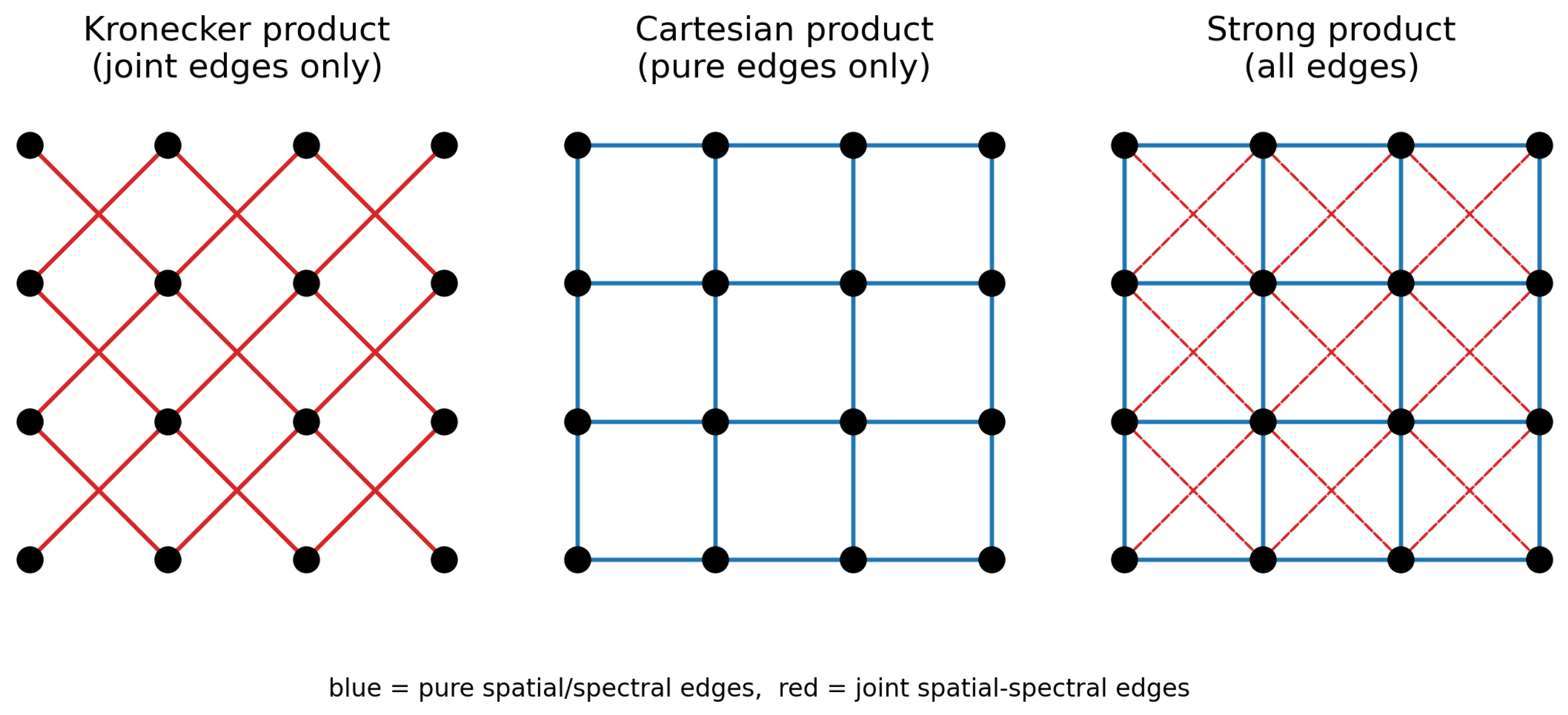
where α , β 0 and the ordering A p A c matches the column-major vectorization of an M N × p block. The first bracket collects the pure-spectral and pure-spatial edges, whereas the second term contains the joint spatial–spectral edges. This family contains the three canonical products as exact special cases (Figure 3):
( α , β ) = ( 0 , 1 ) : Kronecker ; ( 1 , 0 ) : Cartesian ; ( 1 , 1 ) : strong , with A 1 , 1 = ( A p + I p ) ( A c + I M N ) I .
The Kronecker product ( α = 0 ) keeps only joint edges and discards the pure edges, which is exactly the edge deficiency of the graph used in [38]. The proposed WSPGLR fixes α = 1 (pure edges always present) and treats β as a single interpretable weight on the joint edges; for 0 β 1 , it therefore spans the Cartesian ( β = 0 ) and strong ( β = 1 ) products and interpolates between them. The regularizer uses the symmetric normalized Laplacian L α , β of (2), so that all graphs share the normalized spectral range [ 0 , 2 ] , avoiding an unnormalized scale confound, while differing in their edge sets and relative weights:
R WSPGLR ( x ) = x L 1 , β x .
This nonnegative quadratic form is a graph-smoothness energy (a squared Laplacian seminorm), not a norm. Because A c contains only (weighted) 4-neighbor edges, L 1 , β is sparse; with a hard boundary cut ( w b = 0 ) it would moreover decouple across superpixels.

3.4. Denoising Model

We combine a global low-rank prior on the clean image (which captures the whole-scene spectral subspace) with the WSPGLR smoothness prior (4) and a sparse noise term:
min X , S X * + λ 1 R WSPGLR ( X ) + λ 2 S 1 s . t . O = X + S , rank ( X ) r ,
where R WSPGLR ( X ) = vec ( X ) L 1 , β vec ( X ) . Splitting the nuclear norm from the graph term with an auxiliary variable F = X gives
min X , S , F F * + λ 1 R WSPGLR ( X ) + λ 2 S 1 s . t . O = F + S , X = F , rank ( F ) r .

3.5. ADMM Solver

The augmented Lagrangian of (6), with multipliers Λ, Γ and penalty μ > 0 , is
L = F * + λ 1 R WSPGLR ( X ) + λ 2 S 1 + Λ , O F S + Γ , X F + μ 2 O F S F 2 + X F F 2 .
ADMM minimizes the blocks in Gauss–Seidel order.
(1)
Low-rank F (truncated singular-value thresholding):
F k + 1 = D 1 / ( 2 μ ) 1 2 O S k + X k + Λ k + Γ k μ , rank r ,
with D τ ( Z ) = U diag ( max ( σ i τ , 0 ) ) V .
(2)
Graph smoothing X (one sparse linear system):
2 λ 1 L 1 , β + μ I vec ( X k + 1 ) = vec ( μ F k + 1 Γ k ) ,
solved by conjugate gradients; the system is sparse (at most 15 non-zeros per row, Section 3.6) and costs one sparse solve per iteration. Only L 1 , β changes with β /graph type, so all variants share the same complexity.
(3)
Sparse S (soft-thresholding):
S k + 1 = S λ 2 / μ O F k + 1 + Λ k / μ .
(4)
Multipliers: Λ k + 1 = Λ k + μ ( O F k + 1 S k + 1 ) and Γ k + 1 = Γ k + μ ( X k + 1 F k + 1 ) , with μ min ( ρ μ , μ max ) . Iteration stops when O F S F / O F ε 1 and X F ε 2 , or when the iteration budget is reached; the clean HSI is X ^ = F .
Algorithm 1 summarizes the procedure.
Algorithm 1: WSPGLR for HSI mixed-noise removal
Input: 
noisy O ; rank r; λ 1 , λ 2 ; balance β .
  • PCA first component → SLIC superpixels → spatial graph A c ; band path graph A p .
  • Build the normalized weighted product-graph Laplacian L 1 , β from (2).
  • Initialize F = X = S = Λ = Γ = 0 , μ = 10 2 .
  • repeat: update F , X , S by (8),(9),(10); update Λ, Γ, μ ; until the stopping criterion or iteration budget is reached.
Output: 
denoised HSI X ^ = F .

3.6. Computational Complexity

The per-iteration cost of Algorithm 1 is dominated by two operations. The low-rank update (8) is an economy-size SVD of an M N × p matrix, O ( M N p 2 ) (or the truncated HOSVD update of Section 3.8, whose Gram matrices cost O M N p ( M + N + p ) but remain small in practice). The graph update (9) is a conjugate-gradient (CG) solve with the sparse matrix 2 λ 1 L 1 , β + μ I : every node of the pixel–band lattice has at most 4 spatial, 2 spectral and 8 joint neighbors, so the system matrix has at most 15 non-zeros per row independently of the image size, and each CG iteration costs O ( M N p ) . With a fixed CG tolerance the overall per-iteration cost is therefore O M N p 2 + K CG M N p and the memory footprint of the Laplacian is at most 15 M N p non-zeros. With a hard boundary cut ( w b = 0 ), A c becomes block-diagonal across superpixels and the solve additionally parallelizes over superpixels; the default soft weighting ( w b = 0.2 ) keeps the same per-row sparsity bound. Measured single-scene runtimes are reported in Section 4.3.

3.7. Optional Edge-Preserving Refinement

The graph term in (5) is a quadratic (Tikhonov) smoother; on piecewise-smooth scenes an additional total-variation prior can further suppress residual noise. We therefore optionally apply one edge-preserving TV step [10] to the reconstruction X ^ , with a weight η selected by the validation protocol of Section 4.3. Crucially, this weight is scene-adaptive and increases with scene smoothness: the validation selects η = 0 on the most detailed scene (WDC, all cases, whose results are therefore produced by the graph model alone), a small weight on Pavia ( η = 0 or 0.008 ) and larger weights on the smooth Indian scene ( η up to 0.015 ). The refinement is thus a scene-adaptive add-on and does not affect the ablation of Section 4.5, which is performed without it.

3.8. Modular Low-Rank Term: A Tensor Extension (WSPGLR-T)

The low-rank block of (6) can be replaced by a Tucker-rank constraint, with the corresponding change to the F -update. The weighted product-graph term and the remaining updates are unchanged. As an instance we define WSPGLR-T, which constrains F (reshaped to M × N × p ) to a Tucker rank ( r 1 , r 2 , r 3 ) ; the F -update becomes a truncated higher-order SVD approximation of the same target matrix as in (8). This replaces the nuclear-norm penalty and matrix-rank constraint with a Tucker-rank constraint. Truncated HOSVD is generally not the exact best approximation at the prescribed multilinear rank, so this variant uses an approximate low-rank update. This yields a direct, controlled comparison of matrix and Tucker low-rank blocks under the same weighted product graph (Section 4.7); the original LRTDTV [12] result is reported separately as same-noise context, not as an otherwise matched ablation.

4. Experiments

4.1. Datasets, Noise and Metrics

Simulated experiments use three cubes spanning two scene types: two detailed urban scenes—a 200 × 200 × 191 region of Washington DC Mall (WDC, Purdue MultiSpec, https://engineering.purdue.edu/~biehl/MultiSpec/hyperspectral.html; accessed on 9 September 2026) and a 200 × 200 × 103 region of Pavia University—and one smooth agricultural scene, the 145 × 145 × 224 simulated Indian Pines cube (Pavia and Indian Pines both from the GIC hyperspectral scene collection, https://www.ehu.eus/ccwintco/index.php/Hyperspectral_Remote_Sensing_Scenes; accessed on 9 September 2026), all normalized to [ 0 , 1 ] . Four mixed-noise cases, all instances of the degradation model (1), follow the direct baseline [38] so that the main quantitative comparison (Section 4.4) uses the same noise protocol: Case 1 equal-variance Gaussian σ = 0.025 + impulse p = 0.05 ; Case 2 equal σ = 0.1 + p = 0.2 ; Case 3 band-varying σ [ 0 , 0.2 ] + impulse [ 0 , 0.2 ] ; Case 4 is Case 3 plus dead lines, which corrupt random columns (width 1–3 px, 3–10 columns per affected band) to zero in 40 % of bands, chosen independently of Case 3’s per-band severity draw. Cases 1–4 span the same range of severities used across the compared low-rank/graph literature, from Case 1 (mild) up to Cases 2–4, which are a deliberate stress test rather than typical operating conditions; Section 4.6 adds a lower-severity and a physically motivated signal-dependent regime to confirm the reported gains do not depend on this severity range. WDC settings are repeated over two noise realizations (mean ± std). Real experiments use the HYDICE Urban and GF-5 Baoqing scenes, with GF-5 Shanghai and AVIRIS Cuprite (JPL AVIRIS data portal, https://aviris.jpl.nasa.gov/data/index.html; accessed on 9 September 2026; a different sensor family) added in Section 4.9 as further real-scene validation. We report Mean PSNR (MPSNR), Mean SSIM (MSSIM), ERGAS and Spectral Angle Mapper (SAM); real data (no ground truth) are assessed visually and by the no-reference diagnostics of Section 4.9 (method noise, stripe jitter, structure leakage). In the tables, ↑ indicates that larger values are better and ↓ indicates that smaller values are better.

4.2. Implementation and Baselines

For the simulated benchmarks, SLIC uses compactness 0.08 and targets one segment per 56 pixels, with a minimum of 120 segments. WSPGLR processes all p bands jointly. The matrix rank is r = 5 for WDC and Pavia and r = 8 for Indian Pines. Unless stated, λ 2 = 0.15 , β = 0.25 , boundary weight w b = 0.2 with bilateral modulation, symmetric normalized Laplacian, ρ = 1.5 , μ max = 10 6 ; λ 1 and the refinement weight η are selected per case by the supervised validation protocol of Section 4.3 and shared across all graph variants for fairness. We compare against three methods run from the authors’ original MATLAB code—LRTV [10], LRTDTV [12], and LLRGTV [13]—and three controlled baselines implemented in Python: a global RPCA control inspired by LRMR [4], a subspace-RPCA-TV control inspired by FastHyDe [15], and a matched Kronecker-graph control inspired by KGLRSSBS [38]. They are not claimed to reproduce the published LRMR patch grouping, the original FastHyDe eigen-image denoiser, or KGLRSSBS’s local superpixel-body and overlapping-band solver; implementation-accurate control names are therefore used in every numerical table and figure. The matched Kronecker control intentionally uses the same global-low-rank/sparse formulation and solver as WSPGLR, with only the product graph changed, so it isolates the proposed graph contribution; comparisons against the three original-code methods remain full-method comparisons. Table 1 lists the implementation used for every method. The comparison is deliberately training-free and model-based: deep and self-supervised denoisers [19,20,21,22,23] operate in a different regime—they require external training data or per-scene optimization on a GPU—whereas our contribution is a regularizer within the model-based family, so the comparison targets that family and, in particular, the matched Kronecker control. We nonetheless add five additional baselines on identical inputs and metrics. Four are learned methods evaluated outside their training domain with no retraining: HSDT [44], a 2023 spectral-attention transformer, run with its released hsdt_l_complex checkpoint (trained on 31-band ICVL data under a complex synthetic-noise protocol) in its flex attention mode, which replaces the checkpoint’s fixed 31-band linear projection with a band-count-agnostic dot-product attention and lets the same weights run unmodified on our 103–224-band cubes; and QRNN3D [21], a 2021 quasi-recurrent 3-D network run with its complex checkpoint (also 31-band ICVL training, but under a noise protocol—impulse, stripe and dead-line corruption combined with Gaussian noise—closer in spirit to our own Cases 1–4 than HSDT’s), whose fully convolutional, band-count-agnostic architecture requires no adaptation at all. The third is MP-HSIR [48], an ICCV 2025 universal HSI-restoration transformer, run with the authors’ remote-sensing checkpoint and complex-noise prompt. Because that released checkpoint has fixed 100-band input/output layers, we cover each full cube by consecutive 100-band windows with 50-band stride and average overlapping estimates; this explicit inference adaptation uses no target-scene training or parameter selection. The fourth is S2TDM [43], first published online in 2025 and assigned to a 2026 volume, and is a spatial–spectral transformer diffusion model. We use its released model_complex checkpoint and the paper’s 10-step sampling schedule; because the checkpoint is trained for 31-band ICVL cubes, each complete test cube is processed using 31-band windows with 16-band stride and overlap averaging, with no target-scene retraining or parameter selection. This adds a recent diffusion family under exactly the same input cubes, noise realizations, and four evaluation metrics. The fifth baseline is 2026 PCC-GLR [40], a model-driven denoiser that combines global and local Pearson spectral graphs with low-rank and sparse-noise terms. We run the released MATLAB code with the authors’ demo parameters unchanged (including its shallow FGLR initialization, local-window settings and BM3D eigen-image step), without test-ground-truth tuning. Table 2 reports the resulting comparison on all three simulated datasets and all four noise cases. All five additional baselines trail WSPGLR on MPSNR in every one of the 12 dataset × case combinations (WSPGLR also leads ERGAS in 11/12 and SAM in 9/12); the MPSNR margin over the strongest additional baseline ranges from 0.47 to 5.88 dB (3.17 dB on average). These are cross-domain checkpoint results: the differences reflect both mismatch between the released training distributions and our test scenes/noise mixtures and, where required, the disclosed fixed-band inference adaptations. They therefore characterize the robustness of released models under this protocol, not a general ranking of the architectures. Section 4.8 provides a complementary comparison in RND’s native evaluation domain. We also ablate the graph-product type.

4.3. Reproducibility and Runtime

Noise realizations and in-house stochastic steps use fixed random seeds (NumPy default_rng or explicit fixed seeds, as applicable). Table 2 uses seeds { 0 , 1 , 2 } for every dataset–case pair; Table 3, Table 4 and Table 5 retain seeds { 0 , 1 } for WDC and seed 0 elsewhere, as stated in their captions. Released third-party implementations retain their original initialization behavior; the corresponding inputs, outputs and run logs are archived with the seed lists to support reproducibility. ADMM uses μ 0 = 10 2 , ρ = 1.5 and 16 iterations, with ε 1 = ε 2 = 10 4 for possible early stopping; the CG solver uses relative tolerance 10 4 with at most 60 inner iterations. Parameter selection on the simulated benchmark is supervised (it uses the simulated ground truth), with the criterion MPSNR + 100 × MSSIM—the 100 × factor is a fixed heuristic that puts MSSIM’s [ 0 , 1 ] range on a scale comparable with MPSNR in dB, so neither metric is numerically negligible. We repeated the full-resolution, held-out two-stage selection with coefficients 50, 100 and 150. Across the 12 dataset–case combinations, all three coefficients select the same ( λ 1 , η ) pair in 10 cases; only Pavia Case 1 (coefficient 50 selects 0.25 / 0 , while 100 and 150 select 0.4 / 0 ) and Indian Pines Case 2 (coefficients 50 and 100 select 0.25 / 0.015 , while 150 selects 0.4 / 0.015 ) differ. Thus, 100 is retained as the middle scale-balancing convention rather than claimed as a unique optimum. Specifically, λ 1 is selected from { 0.12 , 0.25 , 0.4 } on a held-out noise realization drawn with seed 1000 and never reported; the test realizations use only seeds 0–2. The refinement weight η is selected from { 0 , 0.008 , 0.015 , 0.025 } on the same held-out seed-1000 realization for WDC, Pavia and Indian Pines; none of these validation realizations enters a reported test average. The selected values are then fixed, shared across all graph variants, and reused unchanged for every test realization. On the real scenes no ground truth is available and no per-scene tuning is performed: all parameters keep the defaults of Section 4.2 ( λ 1 = 0.25 , no refinement). Experiments ran on a 48-core Intel Xeon Gold 6248R (3.0 GHz, 125 GB RAM) using Python 3.11.7 and NumPy 1.26.4 (baselines LRTV, LRTDTV and LLRGTV were run with the authors’ original MATLAB code under GNU Octave 5.2; PCC-GLR was run from its released code under MATLAB R2021a). As disclosed in the Acknowledgments, Codex CLI assisted code prototyping, data-analysis scripting and language editing; the authors reviewed the generated code, analyses and text.
Table 1 reports measured runtimes: restoring the pure edges costs only ∼23% more time than the matched Kronecker control (the Laplacian gains joint and pure entries but keeps its bounded per-row sparsity). The memory cost of the extra edges is proportionally larger than the time cost (∼48% more peak RSS than the matched Kron-control, 6.4 GB versus 4.3 GB on this 200 × 200 × 191 cube): both graphs solve the same sparse linear system via conjugate gradients, but our implementation stores the Cartesian and joint blocks of L 1 , β as separate sparse factors before summing them, so the weighted product graph briefly holds more sparse-matrix data than the Kronecker graph’s single term; fused assembly could reduce this temporary storage. The Kronecker and WSPGLR CPU runtimes are directly comparable (both pure Python on the same hardware); the MATLAB/Octave figures are reported for context only and should not be read as a language-level efficiency claim, and the CUDA rows are likewise device-specific inference measurements rather than direct algorithmic comparisons with the CPU rows.

4.4. Quantitative Results

Table 3, Table 4 and Table 5 report WDC, Pavia and Indian Pines, and Table 6 summarizes the average rank of each method. Throughout, WSPGLR denotes the pure graph model—our main method—and WSPGLR+TV the optional post-processed variant of Section 3.7; on WDC the validation selected η = 0 in every case, so the two rows coincide there, whereas small positive weights were selected on Pavia (Cases 2–4) and on Indian (Section 3.7)—every conclusion about the graph itself refers to the WSPGLR rows, which are reported for all datasets. On the detailed urban scenes (WDC, Pavia) WSPGLR attains the best MPSNR against the external methods and matched control in seven of eight settings, is non-leading in several MSSIM and SAM comparisons, and improves MPSNR and ERGAS over the matched Kronecker control in every case of every dataset (MSSIM in 11 of the 12 settings, the exception being Pavia Case 2, where it is 0.859 versus 0.865), with a graph-term-alone margin of up to 2.5 dB MPSNR (Indian Case 4, Table 5); the SAM results, however, reveal a spatial–spectral trade-off—the Kronecker graph, whose joint edges act as a strong spectral smoother, retains a small SAM advantage on WDC (Section 4.5). On the smooth agricultural scene (Indian) the tensor-TV method LRTDTV—whose global tensor factorization is well matched to piecewise-smooth data with pronounced low-rank structure—leads; there the TV refinement, which shares the same piecewise-smooth prior, recovers part of the gap (WSPGLR+TV ranks second and surpasses the global-RPCA and subspace-RPCA-TV controls, LLRGTV and the matched Kronecker control), but we attribute this gain to the post-processing, not to the graph. Thus, no single competitor is uniformly strong: LRTDTV excels on smooth scenes but trails WSPGLR by up to 3.3 dB on detailed scenes. By the average rank of Table 6, the pure graph model attains the best MPSNR and ERGAS ranks among the competing baselines while uniformly improving the MPSNR of the superpixel/band-segmented framework it builds on, and the post-processed WSPGLR+TV additionally attains the best overall rank.
The average-rank summary in Table 6 separates the two contributions. The pure graph model WSPGLR attains the best MPSNR and ERGAS ranks among the competing baselines and improves the overall rank of its matched Kronecker control from 4.62 to 3.58; the optional post-processing then lifts WSPGLR+TV to the best overall rank (2.21), while LRTDTV remains strongest on SAM. This supports the intended interpretation: the graph itself delivers the spatial-reconstruction gains, the TV step is a scene-adaptive complement, and neither variant is uniformly dominant on every individual metric.

4.5. Ablation: Which Edges Matter

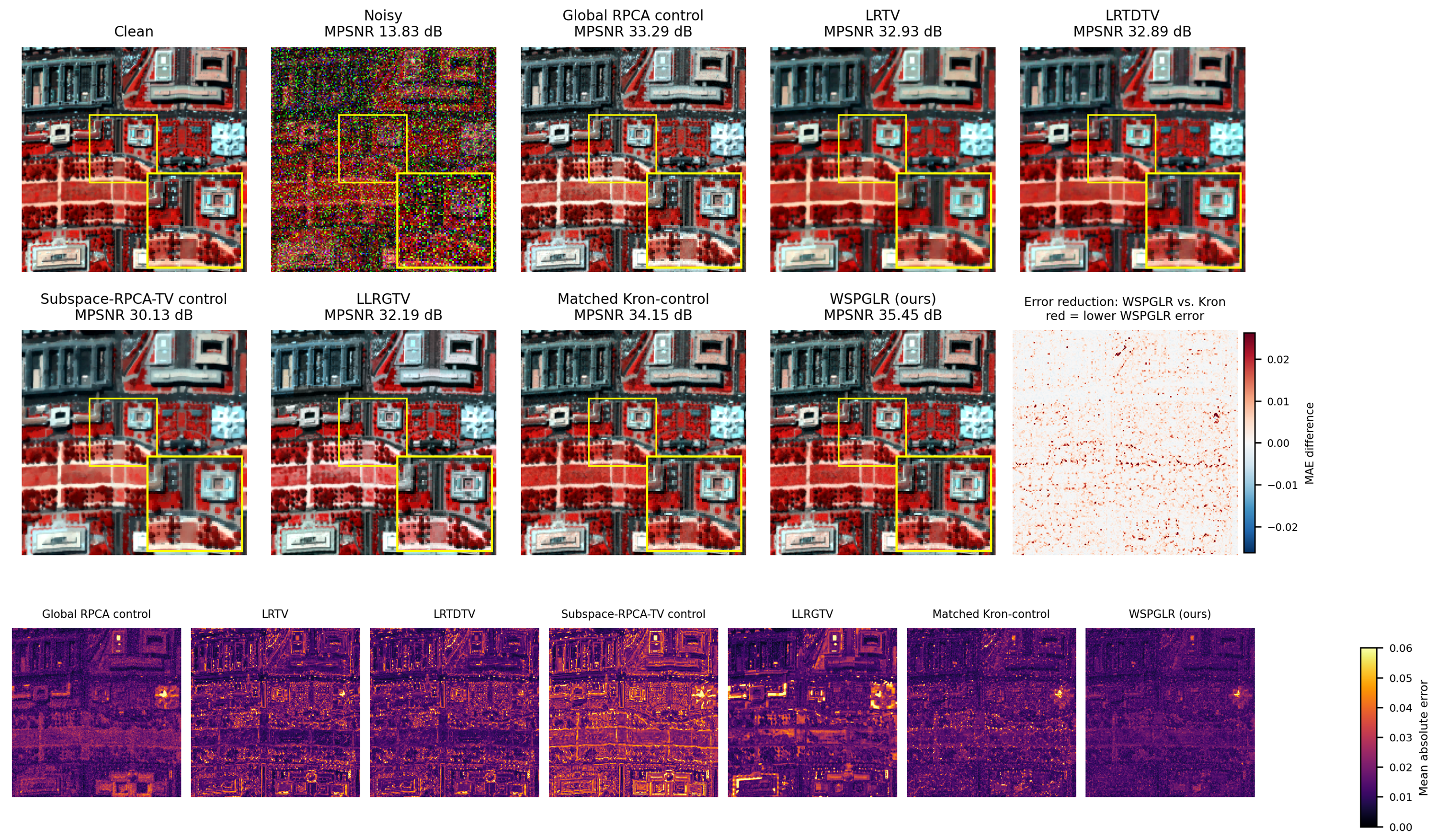
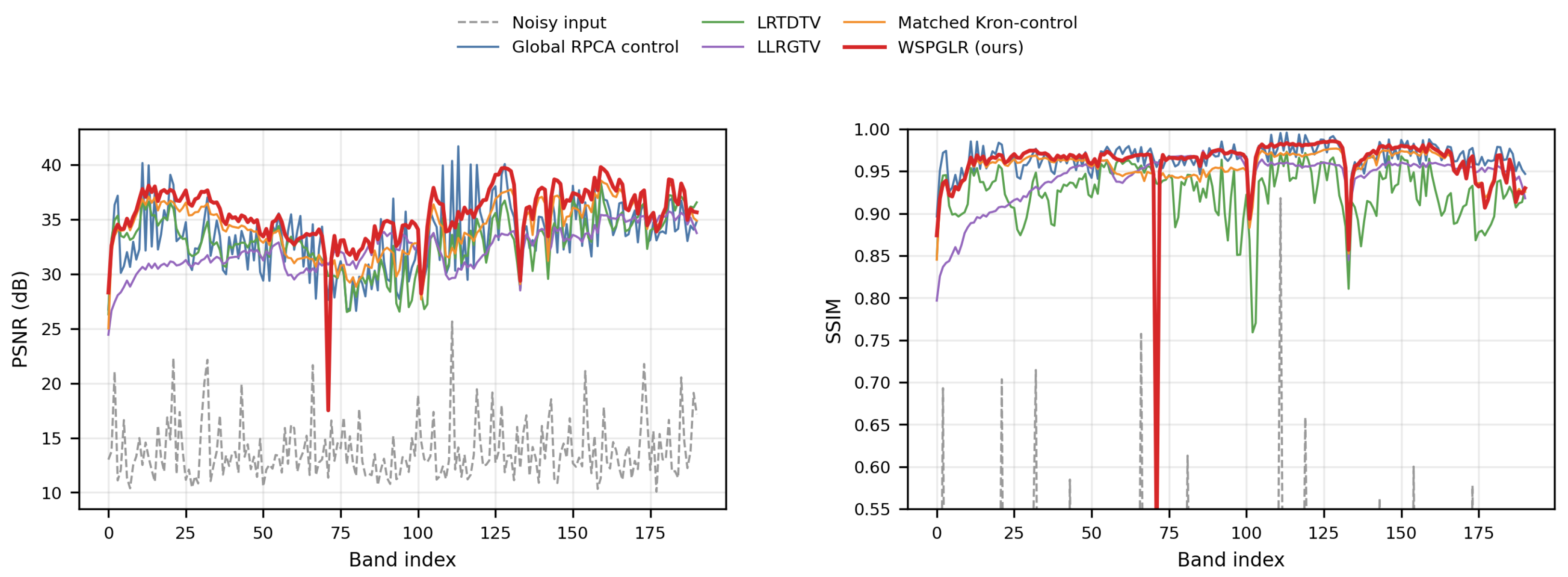
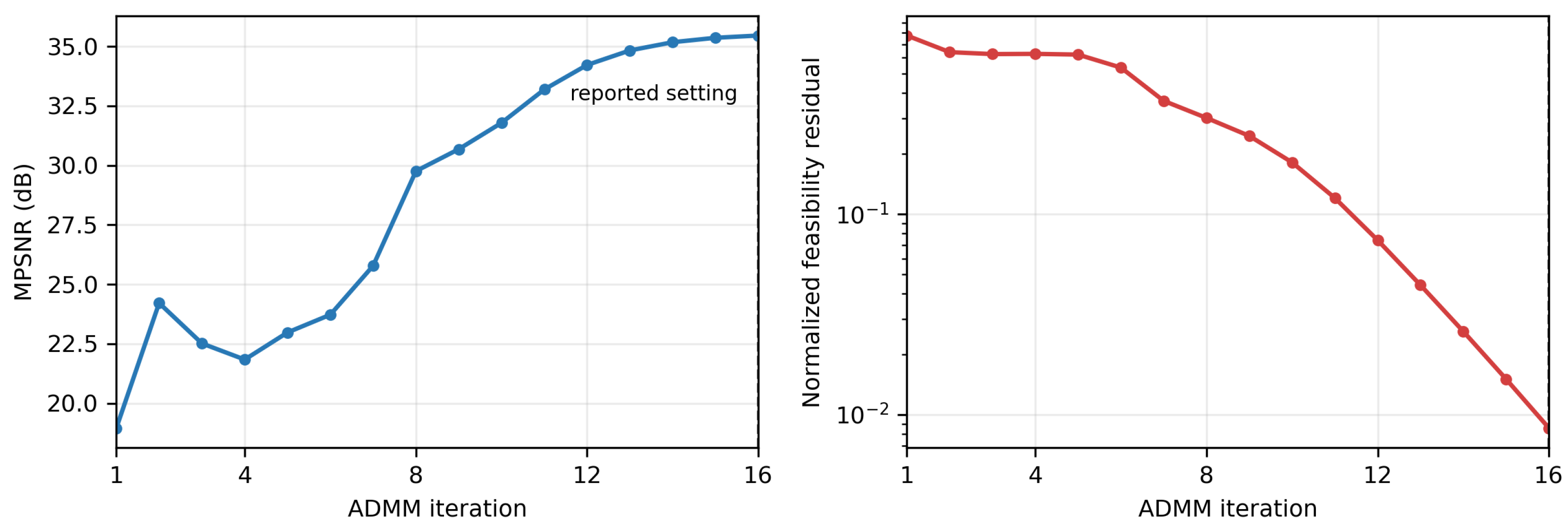
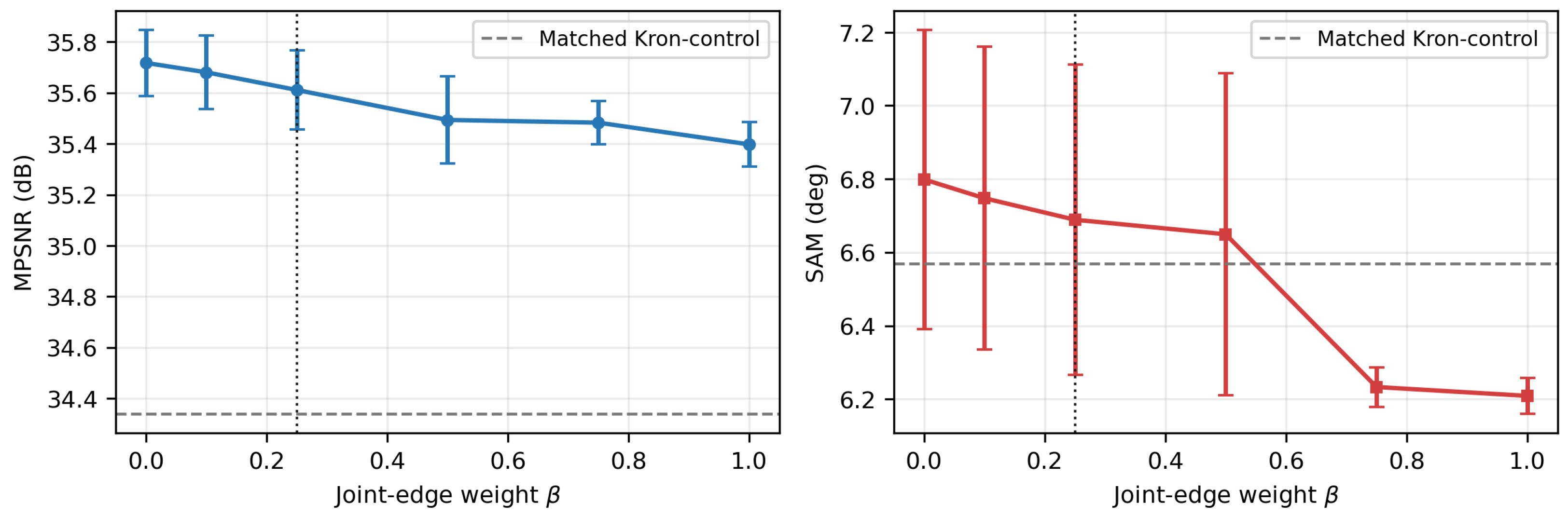
Figure 4 compares the restored images and error maps; Figure 5 reports band-wise quality; Figure 6 shows iteration behavior; and Figure 7 examines the joint-edge weight.
Table 7 changes only the product graph while keeping the model, solver and hyperparameters fixed. The Kronecker graph (joint edges only) attains the worst PSNR/SSIM/ERGAS but, interestingly, the best SAM: its joint spatial–spectral edges act as a strong spectral smoother. Restoring the pure-spatial and pure-spectral edges (the Cartesian, Strong and WSPGLR graphs) lifts PSNR by up to 1.4 dB on WDC and by up to 2.8 dB on the other datasets and markedly improves SSIM/ERGAS, at a small SAM cost. Thus the product-graph type governs a spatial–spectral fidelity trade-off: pure edges favour spatial reconstruction, joint edges favour spectral fidelity. Within the strong-product family the effect of the balance weight β on PSNR is mild (Figure 7); β = 0.25 offers a favourable PSNR–SAM balance and is adopted as the default, retaining essentially all of the PSNR gain of the pure edges while tempering the SAM cost. Figure 7 sweeps β on WDC only; Table 8 repeats the sweep on all three datasets (Case 3, fixed λ 1 per dataset, no TV refinement) to check whether the default needs per-dataset re-tuning. The trade-off strength itself is scene-dependent: on WDC, MPSNR falls only mildly ( 35.72 35.40 dB, β = 0 1 ) while SAM improves ( 6.80 ° 6.21 ° ), so a SAM-sensitive urban application could reasonably push β higher; on Pavia, SAM is nearly insensitive to β ( 7.39 ° 7.34 ° ), so larger β buys almost nothing there; on the smooth Indian scene, β is not favourable at all—MPSNR falls monotonically and substantially ( 34.25 33.14 dB) for only a marginal SAM gain ( 1.76 ° 1.70 ° ), because Indian’s gains come mainly from the TV refinement (Section 3.7) rather than from the joint-edge term. The fixed default β = 0.25 is therefore a conservative, dataset-agnostic compromise—it never costs more than 0.34 dB MPSNR on any of the three datasets relative to its own best-case β —rather than the optimum for any one scene type; Section 5 turns this into practical tuning guidance.

4.6. Realism Check: Moderate and Signal-Dependent Noise

Cases 1–4 (Section 4.1) follow the direct baseline’s protocol and intentionally span from mild (Case 1) to severe (Cases 2–4) additive noise, so that the main comparison uses the noise protocol of prior work; Cases 2–4 in particular are a stress test; their input MPSNR (10.9–17.9 dB across datasets, Table 3, Table 4 and Table 5) is substantially below the lower-severity regimes considered here. To test whether the WSPGLR-over-matched-control margin persists beyond this severity range and the purely additive model, Table 9 adds two regimes on WDC: a moderate case (band-varying σ [ 0 , 0.05 ] , impulse [ 0 , 0.05 ] ) and a physically motivated signal-dependent case (band-varying Poisson shot noise on a peak photon count of 200–2000 plus a small Gaussian read floor, following the amplitude-dependent noise characterization of [3], with a light impulse component). Both push the input MPSNR up to 21.06 ± 0.37 and 23.21 ± 0.30 dB, respectively, well outside the stress-test range. The graph-only WSPGLR-over-matched-control margin shrinks sharply at this mild severity—from up to 2.5 dB under Cases 1–4 to + 0.072 ± 0.009 and + 0.087 ± 0.003 dB here. MPSNR is already above 42 dB for both methods. The gain is positive for each of the three independently generated test realizations in both regimes, but its small magnitude limits this result to a consistency check rather than a claim of practically large improvement under mild noise.

4.7. Tensor Extension: Modularity and Spectral-Fidelity Diagnostic

Table 10 evaluates WSPGLR-T (Section 3.8), which swaps the matrix nuclear norm and rank constraint for a truncated HOSVD update while keeping the weighted product graph fixed; to isolate the low-rank term, neither variant uses the TV refinement here and all remaining parameters are matched. Three observations emerge. First, the effect of the Tucker prior is scene-dependent but modest: it yields a small PSNR/SSIM gain on the piecewise-smooth Indian cube and a small PSNR cost on the detailed urban scenes, which are not spatially low-rank. Second, the Tucker prior improves the spectral angle in five of the six settings—its spectral-mode truncation acts as an additional spectral regularizer—so WSPGLR-T is the preferable variant when spectral fidelity is the priority. Third, the original-code LRTDTV result provides same-noise context but is not an otherwise matched graph-versus-TV ablation; its stronger Indian result is nevertheless consistent with the fact that an 1 spatial–spectral TV is well matched to piecewise-constant scenes. In the synthetic Indian cube, 93 % of adjacent spatial pixel pairs have a band-averaged absolute clean-image difference below 0.5 % of the dynamic range, whereas the corresponding fractions are only 12 % (WDC) and 5 % (Pavia) for the urban scenes, where both of our variants surpass LRTDTV. This comparison delineates the observed applicability domain and demonstrates that the low-rank block is modular; it does not attribute the full between-method gap to a single regularizer or claim uniform superiority.
In summary, compared with matrix WSPGLR, WSPGLR-T improves SAM in five of the six tested settings at a nearly neutral mean MPSNR change ( 0.01 dB on average); this confirms that the low-rank block is modular and that the Tucker variant is the appropriate choice when spectral fidelity is prioritized.

4.8. Real Paired-Noise Comparison Against a Domain-Trained Deep Denoiser (MEHSI)

Section 4.2’s HSDT comparison (Table 2) evaluates a deep denoiser outside its training domain. For a complementary native-domain comparison on genuine sensor noise, we compare against RND [45], a two-stage physical/implicit-noise-removal framework trained on MEHSI [45] (https://huggingface.co/datasets/YingkaiZhang/MEHSI; accessed on 9 September 2026), a paired real-noise HSI dataset (SOC710-VP camera, 34 bands, three controlled exposure ratios 1/20, 1/50, 1/100 of a fully-exposed reference). We use RND’s released checkpoint and its official test protocol unmodified (center 512 × 512 crop; noisy input rescaled by the exposure ratio; output clamped to [ 0 , 1 ] ) on all 30 official MEHSI test pairs (10 scenes × 3 exposure ratios); WSPGLR uses parameters fixed before testing ( λ 1 = 0.25 , λ 2 = 0.15 , β = 0.25 , r = 5 , no refinement or per-scene tuning), processes all 34 bands jointly, and uses the SLIC rule of Section 4.2. Table 11 reports the result. RND, trained on the MEHSI training split, wins all four metrics by a wide margin on every one of the 30 pairs (mean MPSNR 36.61 vs. 26.98 dB; SAM 2.29° vs. 13.36°). WSPGLR nevertheless improves all four metrics over the raw noisy input on every pair. RND used GPU inference whereas WSPGLR used CPU optimization, so the MEHSI wall-clock measurements are not used for an efficiency comparison; the controlled runtime analysis is reported in Table 1. Together with the cross-domain results in Table 2, this comparison delimits the evidence: WSPGLR is a training-free regularizer, not a claim of general superiority over domain-trained deep denoisers (Section 5).

4.9. Visual, Iteration and Parameter Analysis

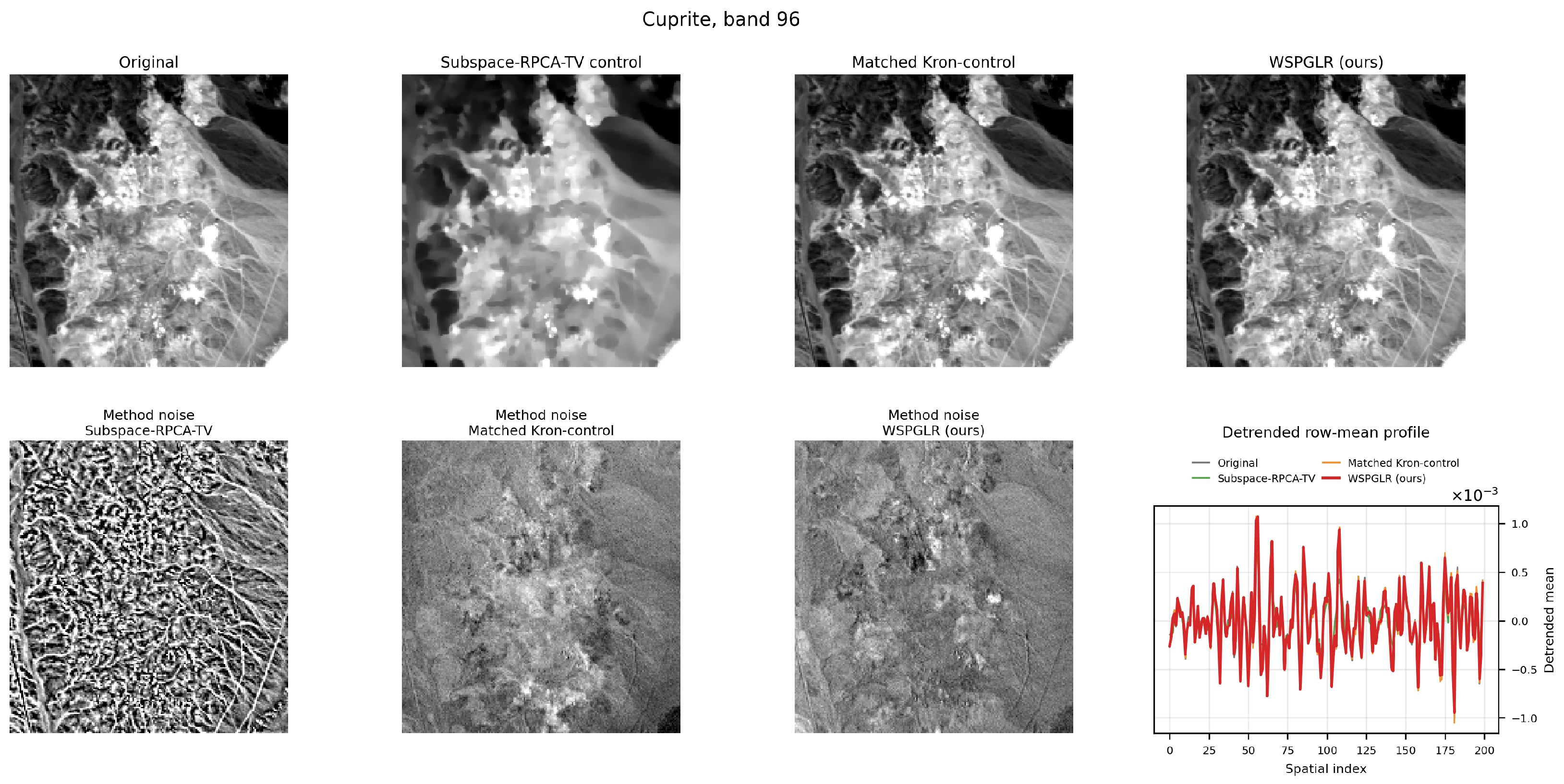
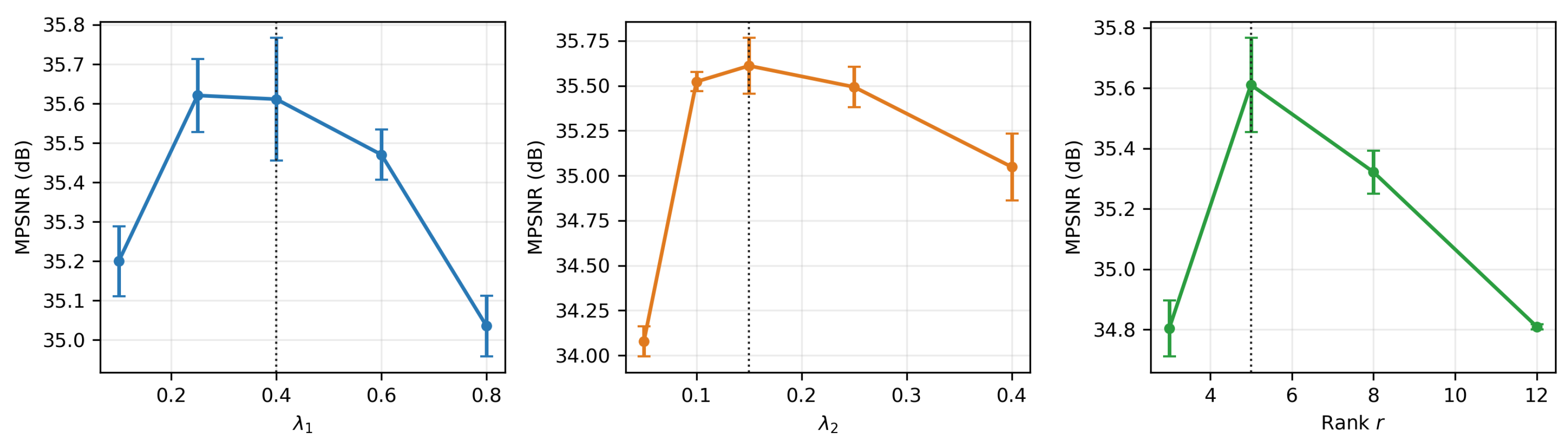
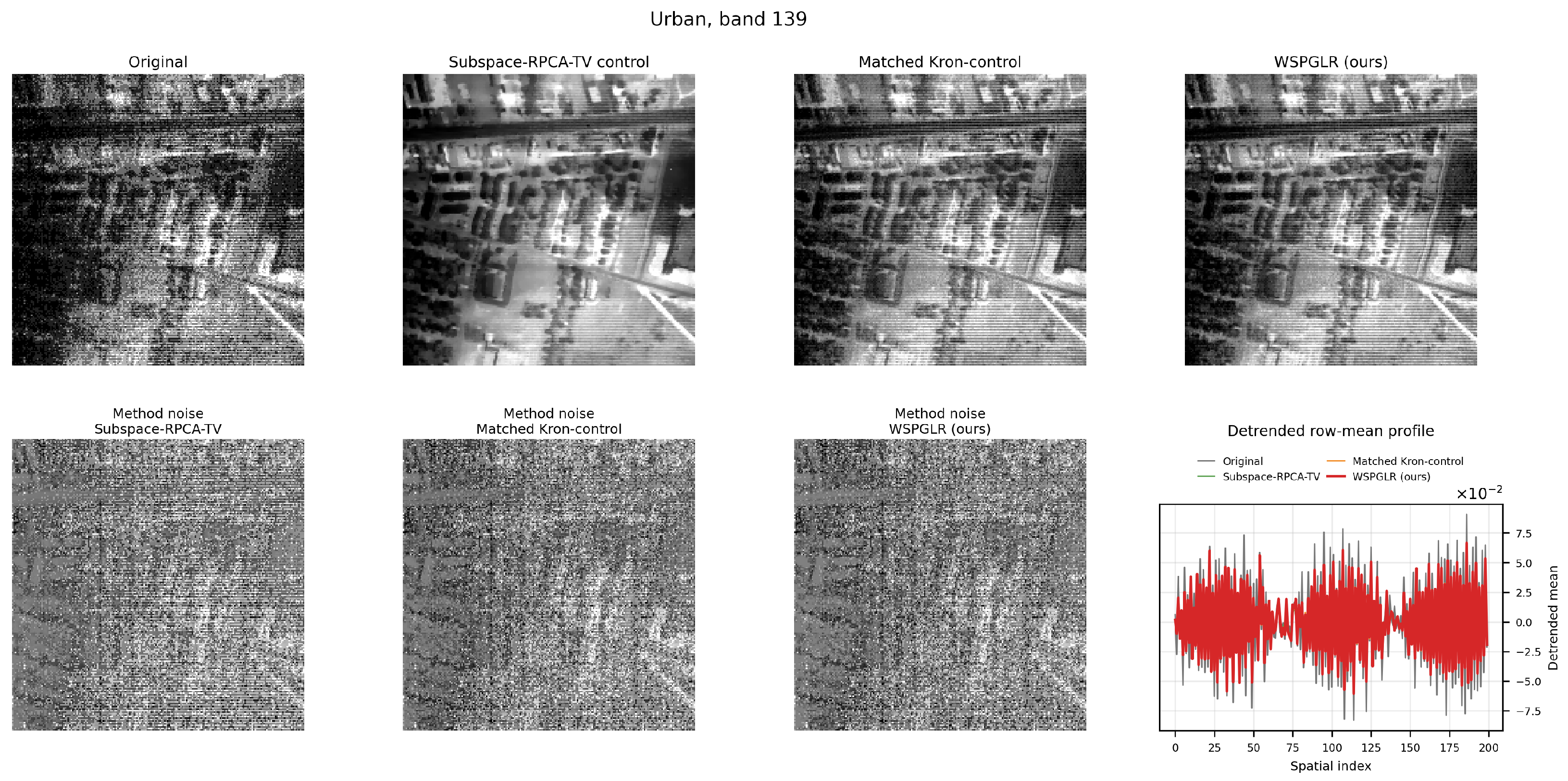
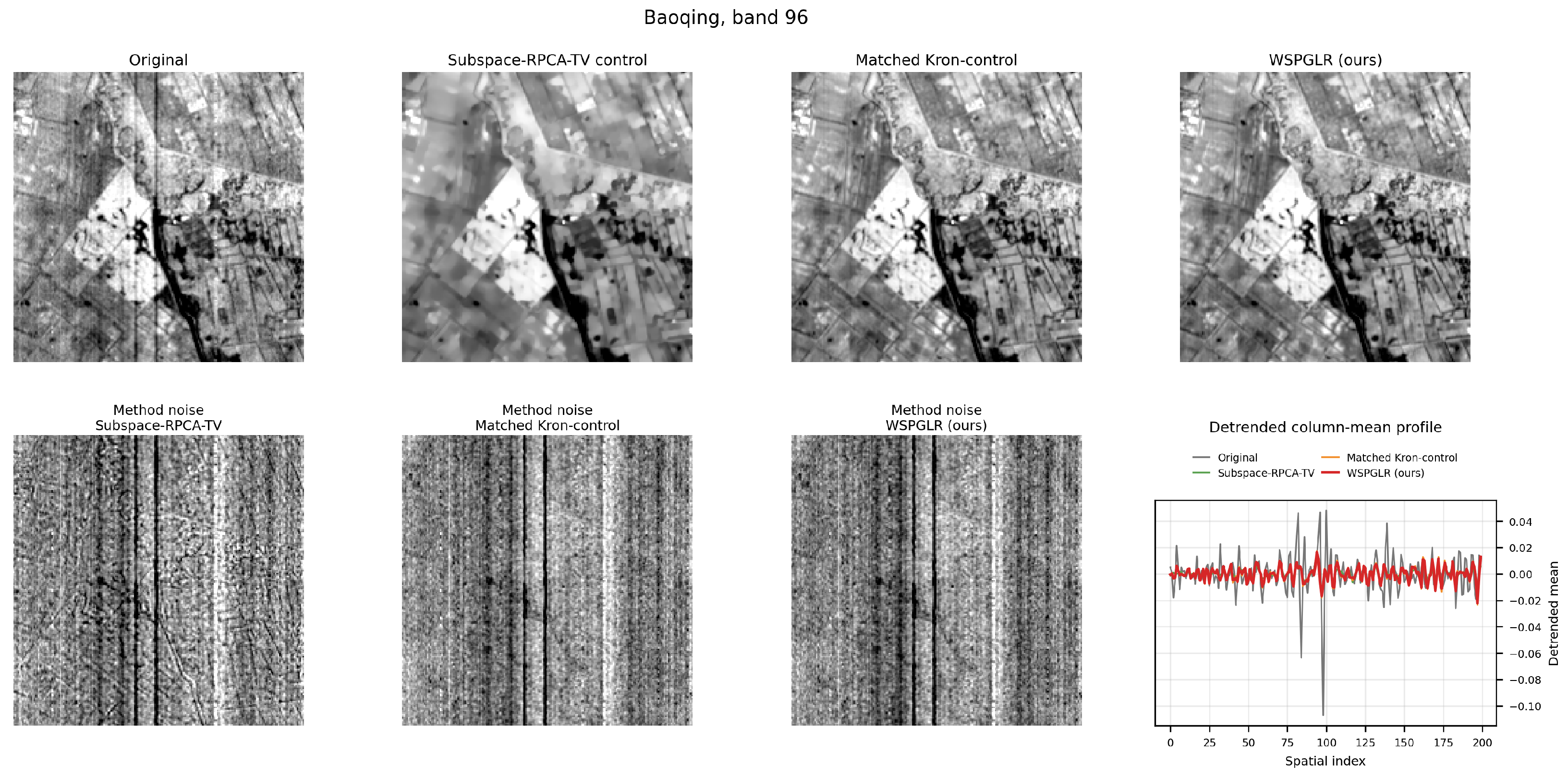
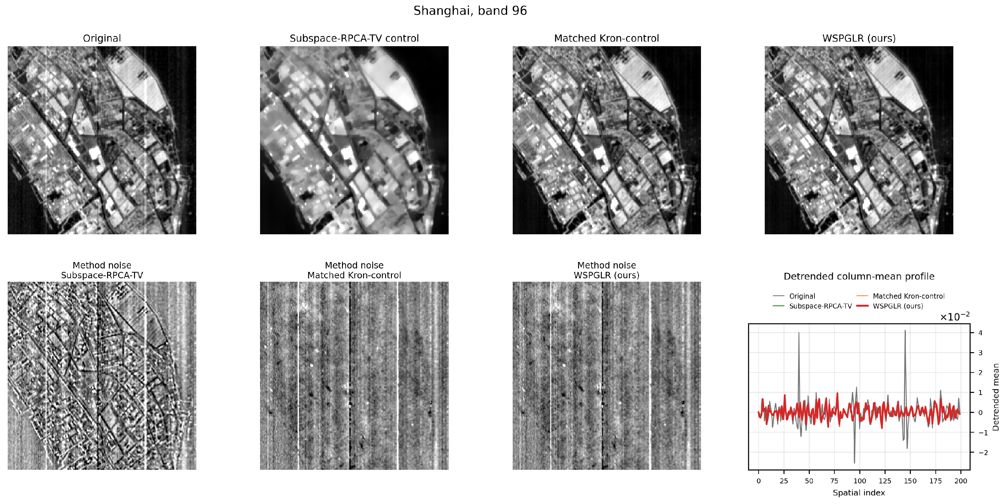
Figure 4 compares reconstructions on WDC Case 3. Because better-performing methods are difficult to distinguish by eye in the restored false-color images, the figure adds band-averaged absolute-error maps on a common color scale: these expose the differences directly, with WSPGLR showing the smallest and least structured error. Figure 5 plots per-band PSNR/SSIM, Figure 6 the iteration behavior of MPSNR and the ADMM feasibility residual under the fixed budget. Figure 7 shows the β sweep. Figure 8, Figure 9, Figure 10 and Figure 11 report real-data results on four scenes across three sensor families—HYDICE Urban, GF-5 Baoqing and Shanghai, and AVIRIS Cuprite. Figure 12 shows sensitivity to λ 1 , λ 2 and r. Since no ground truth exists for the real scenes, we visualize the method noise [49] of each method—the difference between the original and the denoised image, which for an ideal denoiser should contain only noise—and summarize every scene by two no-reference quantities: the residual stripe jitter (mean absolute value of the mean profile taken across the stripe direction after subtracting its 5-tap moving average) and the structure leakage (correlation magnitude between the method noise and the high-pass detail of the corresponding result; pure noise is uncorrelated with scene detail, so this quantifies the classical requirement that the method noise “look like noise” [49]). A good method combines low jitter with low leakage. WSPGLR reduces the jitter from 10.0 × 10 3 to 4.4 × 10 3 on Baoqing and from 38.4 × 10 3 to 29.2 × 10 3 on Urban at near-minimal leakage (0.05–0.10); on the structure-rich Urban crop much of the remaining jitter is genuine one-pixel-scale scene detail rather than stripes, which is why the subspace-RPCA-TV control reaches a lower jitter ( 11.8 × 10 3 ) only at 2.7–6 times the leakage of WSPGLR (0.27–0.32 versus 0.05–0.10)—it removes signal together with the noise, as its method noise confirms. On the two added GF-5 scenes and on AVIRIS Cuprite, the same qualitative pattern holds: structure leakage is 0.053 0.101 for WSPGLR and 0.059 0.113 for the matched Kronecker control across all four scenes (WSPGLR lower on three of four; the matched control is marginally lower on Shanghai, 0.059 versus 0.072 ), while the subspace-RPCA-TV control’s leakage is 0.27 0.60 on every single scene—consistently the highest of the compared methods regardless of sensor or location. Cuprite has comparatively little real striping to begin with (jitter 0.15 0.26 × 10 3 for every method, an order of magnitude below the other three scenes), so there the leakage diagnostic, not stripe suppression, is the informative axis, and it reproduces the same ranking.
Figure 8. Real-data denoising on HYDICE Urban (band 139, horizontal stripes). The top row compares the original band with the subspace-RPCA-TV control, matched Kronecker control and WSPGLR at a common display size. The bottom row gives the three corresponding method-noise maps (original minus result) on a shared ± 2.5 σ scale and a detrended row-mean profile. The numerical jitter/leakage diagnostic is reported in Table 12; the subspace control removes more profile variation but its structured method noise and higher leakage indicate signal loss.
Remotesensing 18 03162 g008
Figure 9. Real-data denoising on GF-5 Baoqing (band 96, vertical stripes). The top row shows the original and three full-size restorations; the bottom row shows their method noise and detrended column-mean profiles. Field boundaries visible in the subspace-RPCA-TV method noise agree with its higher structure-leakage value in Table 12.
Remotesensing 18 03162 g009
Figure 10. Real-data denoising on GF-5 Shanghai (band 96), using the same full-size restoration, method-noise and detrended-profile layout as Figure 8. The scene provides an independent within-sensor check of the Baoqing pattern.
Remotesensing 18 03162 g010
Figure 11. Real-data denoising on AVIRIS Cuprite (band index 96 of 188 good bands after standard water-absorption band removal), using the same layout as Figure 8. Because this band has little inherent striping (jitter 0.16 0.26 × 10 3 ), structure leakage and the method-noise maps are more informative than profile suppression; the subspace control again removes substantial scene structure.
Remotesensing 18 03162 g011
Figure 12. Parameter sensitivity of WSPGLR under the current WDC Case 3 protocol ( 200 × 200 × 191 , 16 ADMM iterations). Points are means over seeds 0 and 1 and error bars are standard deviations; dotted lines mark the reported defaults. Each panel varies only the displayed parameter while holding the others at λ 1 = 0.4 , λ 2 = 0.15 and r = 5 .
Remotesensing 18 03162 g012
Table 12. No-reference diagnostics for the bands displayed in Figure 8, Figure 9, Figure 10 and Figure 11. Each method cell is residual stripe jitter ( × 10 3 )/structure leakage; lower is better for both, but the two quantities must be interpreted jointly because aggressive smoothing can reduce jitter by removing scene structure. ND denotes not defined: the original image has no method-noise residual from which leakage could be computed.
SceneOriginalGlobal RPCASubspace-RPCA-TVMatched Kron-ControlWSPGLR
Urban38.379/ND34.582/0.00911.766/0.26928.633/0.11329.215/0.101
Baoqing10.009/ND3.770/0.1032.343/0.3154.627/0.0614.421/0.053
Shanghai4.007/ND2.185/0.0771.338/0.5152.433/0.0592.474/0.072
Cuprite0.253/ND0.253/0.0100.159/0.5980.261/0.0900.256/0.071

5. Discussion

The ablation clarifies a point left implicit in prior product-graph HSI models: adding pure-spatial and pure-spectral edges to the matched Kronecker control improves MPSNR in the tested settings, while the joint edges influence spectral fidelity. The results do not establish that the strong product is uniformly optimal—the Cartesian member ( β = 0 ) is occasionally the best on PSNR—but that the Kronecker graph is edge-deficient, that the tested pure-edge variants improve upon it on the spatial-reconstruction metrics, and that β selects an operating point on the PSNR–SAM trade-off. The two-parameter product-graph family (2) exposes this cleanly: it contains the Kronecker, Cartesian and strong products as special cases (3), and within the pure-edge branch ( α = 1 ) the single joint-edge weight β lets the operating point trade a small amount of MPSNR for better spectral fidelity. Coupling the graph term with a global low-rank prior—rather than the per-body local low-rank of [38]—is effective on the two urban scenes, while the smooth-scene results expose its scene-dependent limitation. On the detailed urban scenes (WDC, Pavia) WSPGLR attains the best MPSNR against the external methods and matched control in seven of the eight settings (all eight with the TV step), outperforming even the tensor-TV method LRTDTV by up to 3.3 dB (Table 3 and Table 4). On the smooth agricultural scene (Indian Pines) LRTDTV, whose global tensor factorization is well matched to piecewise-smooth data with pronounced low-rank structure, takes the lead; the post-processed WSPGLR+TV ranks second and surpasses the global-RPCA and subspace-RPCA-TV controls, LLRGTV and the matched Kronecker control, while the pure graph model is also non-leading on this scene. More generally, the strongest baselines are scene-dependent: WSPGLR attains the best MPSNR against the external methods and matched control in seven of eight urban settings, is non-leading on Indian Pines, and improves MPSNR over the matched Kronecker control in all 12 settings. Limitations include the non-leading performance on very smooth, low-rank scenes, the reliance on a single global rank, and the optional TV refinement whose weight, although selected by a fixed validation protocol rather than by hand, is an extra hyper-parameter. We also note that WDC results are averaged over two noise realizations, whereas the larger Pavia and Indian tables report a single realization; the WDC standard deviations (Table 3) are small, indicating stable behavior. Table 9 provides an additional three-seed check for the two milder WDC regimes and reports the uncertainty of the small WSPGLR–matched-control margins explicitly. The tensor extension of Section 4.7 already addresses the smooth-scene limitation in part and shows the low-rank term is modular. We also investigated a per-superpixel data-adaptive β estimated from the pure/joint edge-energy ratio of a low-rank pilot; the resulting map is nearly constant across both scene types and does not improve on the fixed global β . This finding limits that particular energy-based rule; it does not exclude benefits from other spatially varying weights. Two further data-adaptive weightings were tested: correlation-based spectral edge weights are uninformative for the same reason (on a low-rank pilot, adjacent-band correlations are near one everywhere), while replacing the first-PC bilateral term by full-spectrum similarity acts as yet another spatial–spectral trade-off knob (on WDC it lowers MPSNR by 0.5 dB but improves SAM by 1.0°; on the smooth scene it is neutral) rather than a free improvement. Edge-adaptive weights, a locally-varying rank, and a broader comparison including non-local and deep denoisers are further natural extensions.

Practical Guidance and Limitations

Tuning β . Table 8 (Section 4.5) shows the PSNR–SAM trade-off controlled by β is scene-dependent rather than a single universal curve. For detailed, spectrally busy scenes (WDC-like), the trade-off is real and worth exploring: β up to 0.75 –1 trades about 0.3 dB MPSNR for a ∼0.6° SAM improvement, which is favourable when downstream spectral analysis (e.g., unmixing or classification) matters more than pixel fidelity. For scenes with flat spectral responses across neighboring pixels (Pavia-like), SAM is nearly insensitive to β , so the default is already close to optimal and increasing β has little to offer. For smooth scenes with pronounced low-rank structure (Indian-like), β is actively unfavorable—MPSNR degrades monotonically for marginal SAM gain—so we recommend β 0.25 , or relying on the TV refinement (Section 3.7) rather than the graph term, for such scenes; this matches the paper’s own finding that Indian’s gains come mainly from the TV step. In the absence of scene-specific tuning, β = 0.25 remains our recommended default: it is never far from the best achievable MPSNR on any of the three scene types tested (Table 8).
Noise-model scope. The main benchmark (Cases 1–4) uses additive, band-varying Gaussian and impulse noise, matching the direct baseline’s protocol; Section 4.6 finds small positive graph-control margins under a milder and a physically motivated signal-dependent (Poisson–Gaussian) regime. We have not evaluated spatially correlated noise (e.g., broader striping patterns than the column/line model of Section 4.1) or noise correlated across adjacent bands beyond the impulse and dead-line components already included.
Real-sensor scope. Section 4.9 now covers four no-reference real scenes across three sensor families (HYDICE Urban; GF-5 Baoqing and Shanghai; AVIRIS Cuprite), and Section 4.8 adds a fourth sensor family (SOC710-VP, via the paired real-noise MEHSI dataset) with genuine ground truth, which is broader than the original two-scene, two-sensor evaluation but still modest relative to the full diversity of operational HSI sensors (e.g., we have not tested ZY-1 02D because suitable raw scenes and reference protocols were not available for this study).
Deep-learning comparison scope. As detailed in Section 2, Section 4.2 and Section 4.8, we now include six additional baselines that characterize both directions of the generalization/specialization trade-off: HSDT, QRNN3D, ICCV 2025 MP-HSIR, S2TDM (online 2025; volume 2026) and model-driven 2026 PCC-GLR (Table 2), each evaluated on the same mixed-noise cubes (the four learned methods are outside their training domains). WSPGLR leads MPSNR in all 12 dataset × case combinations; S2TDM exceeds the other 2025 cross-domain baseline, MP-HSIR, in MPSNR in all 12 settings and wins MSSIM on Indian Cases 2–4, so the comparison also records where its learned prior is advantageous. RND (Table 11), evaluated in its native MEHSI domain on real paired camera noise (MEHSI), outperforms WSPGLR by a large margin while WSPGLR still provides a smaller, consistent improvement over the noisy input. The cross-domain and native-domain results define the evaluation scope of this study and motivate the training-free, no-external-data regime it targets. The controlled 12-case matrix now includes two independently released 2025 same-task methods from distinct learned families (multi-prompt transformer and transformer–diffusion) and the 2026 model-driven PCC-GLR, while the 2026 RND experiment provides the complementary native-domain result. It does not exhaust every 2025–2026 architecture or replace a future benchmark in which all networks are retrained for every sensor and noise model; that broader native-domain comparison remains outside the present study. The added diffusion baseline is a pretrained model; self-supervised diffusion and recent non-local tensor methods have not been evaluated separately.

6. Conclusions

We introduced WSPGLR, a Weighted Strong Product Graph Laplacian Regularizer, that restores the pure spatial–spectral edges omitted by the Kronecker product graph of prior superpixel/band-segmented HSI denoisers, and solved the resulting low-rank plus sparse model with an ADMM combining thresholding steps with a sparse CG solve. Across three simulated scenes, four no-reference real HSIs spanning three sensor families, and 30 paired MEHSI images from a fourth sensor family, WSPGLR consistently improves MPSNR and ERGAS over the matched Kronecker control in every simulated case (and MSSIM in 11 of 12 settings), while the SAM results expose a spatial–spectral fidelity trade-off governed by the joint-edge weight β ; by average rank the pure graph model attains the best MPSNR and ERGAS ranks, and with the optional scene-adaptive TV post-processing the best overall rank, across scene types. An ablation isolates the source of the improvement in the restored pure spatial–spectral edges. A cross-dataset sweep of the joint-edge weight finds scene-dependent behavior; the small positive margins under milder and signal-dependent noise and the real-scene tests broaden the evaluation beyond the main stress-test protocol (Section 4.5, Section 4.6, Section 4.7, Section 4.8, Section 4.9 and Section 5). Six additional baselines broaden the comparison: HSDT, QRNN3D, ICCV 2025 MP-HSIR and S2TDM (online 2025; volume 2026) are run outside their training domain, and 2026 PCC-GLR is run from its released model-driven implementation, on the same 12 mixed-noise settings, where WSPGLR leads MPSNR throughout while S2TDM wins MSSIM on three Indian settings (Table 2); conversely, on real paired camera noise in its native MEHSI domain, RND outperforms WSPGLR by a wide margin, though WSPGLR still improves consistently over the noisy input (Table 11)—together illustrating the generalization/specialization trade-off that motivates a training-free regularizer. Future work will pursue adaptive Tucker ranks, adaptive edge weighting, per-scene rank, and a broader native-domain benchmark in which recent deep priors are retrained for each sensor and noise model.

Author Contributions

Conceptualization, X.L. and X.S.; methodology, X.L. and X.S.; software, X.L. and W.F.; validation, X.L. and J.L. (Jingjing Li); formal analysis, X.L. and Y.J.; investigation, X.L.; data curation, X.L. and W.F.; writing—original draft preparation, X.L.; writing—review and editing, X.S., J.L. (Jingjing Li), Y.J., M.M., W.L., X.J. and J.L. (Jian Liu); visualization, X.L.; supervision, X.S.; funding acquisition, X.S. All authors have read and agreed to the published version of the manuscript.

Funding

This research was funded by the Guangxi Science and Technology Program, grant numbers AA24263010, AB23026120, AA24263006, AA24206043 and AD25069103; the Guangxi Natural Science Foundation, grant number 2024GXNSFBA010265; and the National Natural Science Foundation of China, grant numbers U23A20280, 62471153 and U25A20397.

Institutional Review Board Statement

Not applicable. This study did not involve human participants, animals, personal data or identifiable private information.

Informed Consent Statement

Not applicable. This study did not involve human participants.

Data Availability Statement

The code and data supporting this study are available from the corresponding author upon reasonable request.

Acknowledgments

During the preparation of this manuscript, the authors used Codex CLI 0.152.1 (OpenAI) for code prototyping, data analysis and language editing. The authors reviewed and validated the generated code, analyses, numerical results, and text and take full responsibility for the content of this publication.

Conflicts of Interest

The authors declare no conflicts of interest. The funders had no role in the design of the study; in the collection, analyses, or interpretation of data; in the writing of the manuscript; or in the decision to publish the results.

Abbreviations

The following abbreviations are used in this manuscript:
ADMMAlternating direction method of multipliers
CGConjugate gradient
ERGASErreur relative globale adimensionnelle de synthèse
GSPGraph signal processing
HSIHyperspectral image
MPSNRMean peak signal-to-noise ratio
MSSIMMean structural similarity index measure
PCAPrincipal component analysis
SAMSpectral angle mapper
SLICSimple linear iterative clustering
SSTVSpatial–spectral total variation
TVTotal variation
WSPGLRWeighted strong product graph Laplacian regularization

References

  1. Khan, M.J.; Khan, H.S.; Yousaf, A.; Khurshid, K.; Abbas, A. Modern trends in hyperspectral image analysis: A review. IEEE Access 2018, 6, 14118–14129. [Google Scholar] [CrossRef] [Scilit]
  2. Bioucas-Dias, J.M.; Plaza, A.; Camps-Valls, G.; Scheunders, P.; Nasrabadi, N.; Chanussot, J. Hyperspectral remote sensing data analysis and future challenges. IEEE Geosci. Remote Sens. Mag. 2013, 1, 6–36. [Google Scholar] [CrossRef] [Scilit]
  3. Meola, J.; Eismann, M.T.; Moses, R.L.; Ash, J.N. Modeling and estimation of signal-dependent noise in hyperspectral imagery. Appl. Opt. 2011, 50, 3829–3846. [Google Scholar] [CrossRef] [Scilit] [PubMed]
  4. Zhang, H.; He, W.; Zhang, L.; Shen, H.; Yuan, Q. Hyperspectral image restoration using low-rank matrix recovery. IEEE Trans. Geosci. Remote Sens. 2014, 52, 4729–4743. [Google Scholar] [CrossRef] [Scilit]
  5. He, W.; Zhang, H.; Zhang, L.; Shen, H. Hyperspectral image denoising via noise-adjusted iterative low-rank matrix approximation. IEEE J. Sel. Top. Appl. Earth Obs. Remote Sens. 2015, 8, 3050–3061. [Google Scholar] [CrossRef] [Scilit]
  6. Dabov, K.; Foi, A.; Katkovnik, V.; Egiazarian, K. Image denoising by sparse 3-D transform-domain collaborative filtering. IEEE Trans. Image Process. 2007, 16, 2080–2095. [Google Scholar] [CrossRef] [Scilit] [PubMed]
  7. Maggioni, M.; Katkovnik, V.; Egiazarian, K.; Foi, A. Nonlocal transform-domain filter for volumetric data denoising and reconstruction. IEEE Trans. Image Process. 2013, 22, 119–133. [Google Scholar] [CrossRef] [Scilit] [PubMed]
  8. Renard, N.; Bourennane, S.; Blanc-Talon, J. Denoising and dimensionality reduction using multilinear tools for hyperspectral images. IEEE Geosci. Remote Sens. Lett. 2008, 5, 138–142. [Google Scholar] [CrossRef] [Scilit]
  9. Liu, X.; Bourennane, S.; Fossati, C. Denoising of hyperspectral images using the PARAFAC model and statistical performance analysis. IEEE Trans. Geosci. Remote Sens. 2012, 50, 3717–3724. [Google Scholar] [CrossRef] [Scilit]
  10. He, W.; Zhang, H.; Zhang, L.; Shen, H. Total-variation-regularized low-rank matrix factorization for hyperspectral image restoration. IEEE Trans. Geosci. Remote Sens. 2016, 54, 178–188. [Google Scholar] [CrossRef] [Scilit]
  11. Aggarwal, H.K.; Majumdar, A. Hyperspectral image denoising using spatio-spectral total variation. IEEE Geosci. Remote Sens. Lett. 2016, 13, 442–446. [Google Scholar] [CrossRef] [Scilit]
  12. Wang, Y.; Peng, J.; Zhao, Q.; Leung, Y.; Zhao, X.-L.; Meng, D. Hyperspectral image restoration via total variation regularized low-rank tensor decomposition. IEEE J. Sel. Top. Appl. Earth Obs. Remote Sens. 2018, 11, 1227–1243. [Google Scholar] [CrossRef] [Scilit]
  13. He, W.; Zhang, H.; Shen, H.; Zhang, L. Hyperspectral image denoising using local low-rank matrix recovery and global spatial–spectral total variation. IEEE J. Sel. Top. Appl. Earth Obs. Remote Sens. 2018, 11, 713–729. [Google Scholar] [CrossRef] [Scilit]
  14. Zeng, H.; Huang, S.; Chen, Y.; Luong, H.; Philips, W. All of low-rank and sparse: A recast total variation approach to hyperspectral denoising. IEEE J. Sel. Top. Appl. Earth Obs. Remote Sens. 2023, 16, 7357–7373. [Google Scholar] [CrossRef] [Scilit]
  15. Zhuang, L.; Bioucas-Dias, J.M. Fast hyperspectral image denoising and inpainting based on low-rank and sparse representations. IEEE J. Sel. Top. Appl. Earth Obs. Remote Sens. 2018, 11, 730–742. [Google Scholar] [CrossRef] [Scilit]
  16. Zhuang, L.; Fu, X.; Ng, M.K.; Bioucas-Dias, J.M. Hyperspectral image denoising based on global and nonlocal low-rank factorizations. IEEE Trans. Geosci. Remote Sens. 2021, 59, 10438–10454. [Google Scholar] [CrossRef] [Scilit]
  17. He, W.; Yao, Q.; Li, C.; Yokoya, N.; Zhao, Q.; Zhang, H.; Zhang, L. Non-local meets global: An iterative paradigm for hyperspectral image restoration. IEEE Trans. Pattern Anal. Mach. Intell. 2022, 44, 2089–2107. [Google Scholar] [PubMed]
  18. He, C.; Sun, L.; Huang, W.; Zhang, J.; Zheng, Y.; Jeon, B. TSLRLN: Tensor subspace low-rank learning with non-local prior for hyperspectral image mixed denoising. Signal Process. 2021, 184, 108060. [Google Scholar] [CrossRef] [Scilit]
  19. Yuan, Q.; Zhang, Q.; Li, J.; Shen, H.; Zhang, L. Hyperspectral image denoising employing a spatial–spectral deep residual convolutional neural network. IEEE Trans. Geosci. Remote Sens. 2019, 57, 1205–1218. [Google Scholar] [CrossRef] [Scilit]
  20. Chang, Y.; Yan, L.; Fang, H.; Zhong, S.; Liao, W. HSI-DeNet: Hyperspectral image restoration via convolutional neural network. IEEE Trans. Geosci. Remote Sens. 2019, 57, 667–682. [Google Scholar] [CrossRef] [Scilit]
  21. Wei, K.; Fu, Y.; Huang, H. 3-D quasi-recurrent neural network for hyperspectral image denoising. IEEE Trans. Neural Netw. Learn. Syst. 2021, 32, 363–375. [Google Scholar] [CrossRef] [Scilit] [PubMed]
  22. Li, M.; Liu, J.; Fu, Y.; Zhang, Y.; Dou, D. Spectral enhanced rectangle transformer for hyperspectral image denoising. In Proceedings of the IEEE/CVF Conference on Computer Vision and Pattern Recognition (CVPR), Vancouver, BC, Canada, 17–24 June 2023; pp. 5805–5814. [Google Scholar]
  23. Miao, Y.; Zhang, L.; Zhang, L.; Tao, D. DDS2M: Self-supervised denoising diffusion spatio-spectral model for hyperspectral image restoration. In Proceedings of the IEEE/CVF International Conference on Computer Vision (ICCV), Paris, France, 1–6 October 2023; pp. 12086–12096. [Google Scholar]
  24. Liu, N.; Li, W.; Wang, Y.; Tao, R.; Du, Q.; Chanussot, J. A survey on hyperspectral image restoration: From the view of low-rank tensor approximation. Sci. China Inf. Sci. 2023, 66, 140302. [Google Scholar] [CrossRef] [Scilit]
  25. Shuman, D.I.; Narang, S.K.; Frossard, P.; Ortega, A.; Vandergheynst, P. The emerging field of signal processing on graphs: Extending high-dimensional data analysis to networks and other irregular domains. IEEE Signal Process. Mag. 2013, 30, 83–98. [Google Scholar] [CrossRef] [Scilit]
  26. Ortega, A.; Frossard, P.; Kovačević, J.; Moura, J.M.F.; Vandergheynst, P. Graph signal processing: Overview, challenges, and applications. Proc. IEEE 2018, 106, 808–828. [Google Scholar] [CrossRef] [Scilit]
  27. Hu, W.; Pang, J.; Liu, X.; Tian, D.; Lin, C.-W.; Vetro, A. Graph signal processing for geometric data and beyond: Theory and applications. IEEE Trans. Multimed. 2022, 24, 3961–3977. [Google Scholar] [CrossRef] [Scilit]
  28. Achanta, R.; Shaji, A.; Smith, K.; Lucchi, A.; Fua, P.; Süsstrunk, S. SLIC superpixels compared to state-of-the-art superpixel methods. IEEE Trans. Pattern Anal. Mach. Intell. 2012, 34, 2274–2282. [Google Scholar] [CrossRef] [Scilit] [PubMed]
  29. Liu, Y.; Shan, C.; Gao, Q.; Gao, X.; Han, J.; Cui, R. Hyperspectral image denoising via minimizing the partial sum of singular values and superpixel segmentation. Neurocomputing 2019, 330, 465–482. [Google Scholar] [CrossRef] [Scilit]
  30. Behroozi, Y.; Yazdi, M.; Zolghadre Asli, A. Hyperspectral image denoising based on superpixel segmentation low-rank matrix approximation and total variation. Circuits Syst. Signal Process. 2022, 41, 3372–3396. [Google Scholar] [CrossRef] [Scilit]
  31. Imrich, W.; Klavžar, S. Product Graphs: Structure and Recognition; Wiley: New York, NY, USA, 2000. [Google Scholar]
  32. Sandryhaila, A.; Moura, J.M.F. Big data analysis with signal processing on graphs: Representation and processing of massive data sets with irregular structure. IEEE Signal Process. Mag. 2014, 31, 80–90. [Google Scholar] [CrossRef] [Scilit]
  33. Leskovec, J.; Chakrabarti, D.; Kleinberg, J.; Faloutsos, C.; Ghahramani, Z. Kronecker graphs: An approach to modeling networks. J. Mach. Learn. Res. 2010, 11, 985–1042. [Google Scholar]
  34. Kadambari, S.K.; Chepuri, S.P. Product graph learning from multi-domain data with sparsity and rank constraints. IEEE Trans. Signal Process. 2021, 69, 5665–5680. [Google Scholar] [CrossRef] [Scilit]
  35. Tan, Z.; Zhu, Y.; Liu, B. Learning spatial-temporal feature with graph product. Signal Process. 2023, 210, 109062. [Google Scholar] [CrossRef] [Scilit]
  36. Cai, W.; Jiang, J.; Ouyang, S. Hyperspectral image denoising using adaptive weight graph total variation regularization and low-rank matrix recovery. IEEE Geosci. Remote Sens. Lett. 2022, 19, 5509805. [Google Scholar] [CrossRef] [Scilit]
  37. Cai, W.; Jiang, J.; Qian, J. Large-scale hyperspectral image restoration via a superpixel distributed algorithm based on graph signal processing. IEEE Trans. Geosci. Remote Sens. 2023, 61, 5503517. [Google Scholar] [CrossRef] [Scilit]
  38. Li, H.; Jiang, J.; Zhou, F.; Quan, Y. Hyperspectral image denoising based on superpixel segmentation and band segmentation. J. Xidian Univ. 2024, 51, 122–135. (In Chinese) [Google Scholar]
  39. Ma, M.; Cai, M.; Shen, Y.; Zhou, F.; Jiang, J. Hyperspectral image denoising algorithm via joint low-rank tensor decomposition and product graph modeling. J. Electron. Inf. Technol. 2025, 47, 3951–3966. (In Chinese) [Google Scholar] [CrossRef]
  40. Liu, C.; Yao, Z.; Fang, F. PCC-GLR: Pearson correlation coefficient-based graph Laplacian regularization for hyperspectral image denoising. Opt. Laser Technol. 2026, 196, 114659. [Google Scholar] [CrossRef] [Scilit]
  41. Ma, M.; Jiang, J.; Zhou, F. CGD-based inpainting algorithm for time-varying signals on strong product graph. Circuits Syst. Signal Process. 2024, 43, 457–469. [Google Scholar] [CrossRef] [Scilit]
  42. Fu, G.; Xiong, F.; Lu, J.; Zhou, J. SSUMamba: Spatial–spectral selective state space model for hyperspectral image denoising. IEEE Trans. Geosci. Remote Sens. 2024, 62, 5527714. [Google Scholar] [CrossRef] [Scilit]
  43. Wu, Z.; Chen, Y.; Xiong, J.; Pan, X.; He, W. S2TDM: Spatial–spectral transformer-based diffusion model for hyperspectral image denoising. Geo-spat. Inf. Sci. 2026, 29, 1737–1754. [Google Scholar] [CrossRef] [Scilit]
  44. Lai, Z.; Yan, C.; Fu, Y. Hybrid spectral denoising transformer with guided attention. In Proceedings of the IEEE/CVF International Conference on Computer Vision (ICCV), Paris, France, 1–6 October 2023; pp. 13019–13029. [Google Scholar]
  45. Zhang, Y.; Zhang, T.; Nie, J.; Fu, Y. Real noise decoupling for hyperspectral image denoising. Proc. AAAI Conf. Artif. Intell. 2026, 40, 12925–12933. [Google Scholar] [CrossRef] [Scilit]
  46. Takemoto, S.; Naganuma, K.; Ono, S. Graph spatio-spectral total variation model for hyperspectral image denoising. IEEE Geosci. Remote Sens. Lett. 2022, 19, 6012405. [Google Scholar] [CrossRef] [Scilit]
  47. Yao, J.; Jiang, J.; Zhou, F. Graph total variation and low-rank regularization for heterogeneous change detection. Digit. Signal Process. 2025, 156, 104825. [Google Scholar] [CrossRef] [Scilit]
  48. Wu, Z.; Chen, Y.; Yokoya, N.; He, W. MP-HSIR: A multi-prompt framework for universal hyperspectral image restoration. In Proceedings of the IEEE/CVF International Conference on Computer Vision (ICCV), Honolulu, HI, USA, 19–23 October 2025; pp. 13009–13020. [Google Scholar] [CrossRef] [Scilit]
  49. Buades, A.; Coll, B.; Morel, J.-M. A review of image denoising algorithms, with a new one. Multiscale Model. Simul. 2005, 4, 490–530. [Google Scholar] [CrossRef] [Scilit]
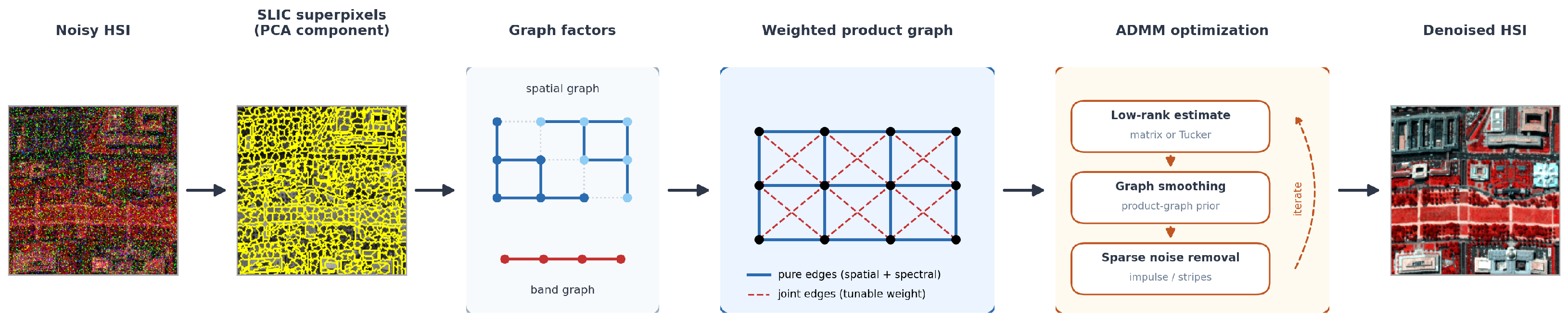
Figure 1. Overview of the proposed WSPGLR framework. The PCA first component of the noisy HSI is over-segmented by SLIC; 4-neighbor edges within superpixels (solid) and soft-weighted boundary edges (dotted) form the spatial graph, while a path graph over adjacent bands forms the band path graph. The two factors are combined into the weighted product graph, whose pure spatial/spectral edges (solid blue) and joint edges (dashed red, tunable weight) instantiate the two-parameter family of Section 3.3; its normalized Laplacian regularizes a global low-rank plus sparse model solved by the three-step ADMM cycle.
Remotesensing 18 03162 g001
Figure 2. PCA first component (left), SLIC superpixels (middle) and the false-color image (right) of a 100 × 100 WDC crop.
Remotesensing 18 03162 g002
Figure 3. Product graphs over the pixel–band lattice. Kronecker keeps only joint (diagonal) edges; Cartesian keeps pure-spatial and pure-spectral edges; the weighted strong product keeps all three, with the joint edges weighted by β . Blue solid lines denote pure edges; red solid lines in the Kronecker panel and red dashed lines in the strong-product panel denote joint edges.
Remotesensing 18 03162 g003
Figure 4. Visual comparison on WDC Case 3 (seed 0; false color) with zoomed insets (yellow boxes). All seven methods are shown with the clean and noisy images, and each result title reports its MPSNR for this realization. The diverging map at right displays the matched-Kronecker minus WSPGLR band-averaged absolute error; red pixels therefore identify locations where WSPGLR lowers the error. The bottom row shows every method’s band-averaged absolute-error map on one common color scale. WSPGLR has the lowest displayed-realization error; the matched Kronecker and global-RPCA controls retain edge-localized errors, while the subspace-RPCA-TV control and LLRGTV show structured over-smoothing and residual noise, respectively.
Remotesensing 18 03162 g004
Figure 5. Per-band PSNR (left) and SSIM (right) on WDC Case 3 for the noisy input and five representative methods. WSPGLR (thick red) is highest over most bands; the sharp dip near band 72 is shared by every method (including the noisy input), so it reflects the band-varying Gaussian/impulse severity of Case 3 drawing an unusually harsh value for that band in this realization—Case 3 itself contains no dead lines (Section 4.1); dead lines are specific to Case 4 and affect approximately 40 % of bands, not a single one.
Remotesensing 18 03162 g005
Figure 6. Iteration behavior of WSPGLR on the current WDC Case 3 protocol ( 200 × 200 × 191 , seed 0, 16 ADMM iterations). (Left) MPSNR versus iteration. (Right) normalized feasibility residual O F k S k F / O F . The residual falls from 0.774 to 0.0086 over the fixed 16-step budget. It measures constraint violation rather than the non-convex objective and is not used to claim asymptotic convergence.
Remotesensing 18 03162 g006
Figure 7. Effect of the joint-edge weight β under the current WDC Case 3 protocol ( 200 × 200 × 191 , 16 ADMM iterations). Points are means over seeds 0 and 1 and error bars are standard deviations. The dashed grey line is the matched Kronecker control and the dotted line marks the fixed default β = 0.25 . Across β [ 0 , 1 ] , mean MPSNR changes by 0.32 dB while mean SAM improves by 0.59°, exposing the intended fidelity trade-off.
Remotesensing 18 03162 g007
Table 1. Measured single-scene runtime and peak memory on WDC Case 3 ( 200 × 200 × 191 , 48-core Xeon 6248R, Intel Corporation, Santa Clara, CA, USA; NVIDIA RTX A6000, NVIDIA Corporation, Santa Clara, CA, USA). Python CPU timings (upper block) are directly comparable; HSDT and QRNN3D use warmed-up single-cube CUDA inference (five warm-up runs, 20 measured runs); S2TDM uses one full-cube warm-up and five measured runs because each inference contains ten diffusion steps over 11 overlapping spectral windows. All GPU timings synchronize before and after each run, include host–device transfers, and report peak allocated GPU memory; LRTV/LRTDTV/LLRGTV run the authors’ original MATLAB code under GNU Octave 5.2 and include interpreter overhead, so their runtimes are indicative only. PCC-GLR reports the mean and population standard deviation of its two WDC Case 3 runs under MATLAB R2021a. Memory was not measured for the MATLAB/Octave methods, since its accounting is not directly comparable with the Python and CUDA values.
MethodRuntime (s)Peak Memory (MiB)Implementation
Global RPCA14879Python (ours)
Subspace-RPCA-TV15881Python (ours)
Matched Kron-control1004305Python (ours)
WSPGLR1236385Python (ours)
HSDT-L-complex 0.658 ± 0.013 5000.8PyTorch/CUDA
QRNN3D-complex 0.413 ± 0.016 4346.8PyTorch/CUDA
S2TDM-complex (2025) 13.235 ± 0.113 454.8PyTorch/CUDA
LRTV133Not measuredoriginal MATLAB/Octave
LRTDTV537Not measuredoriginal MATLAB/Octave
LLRGTV4048Not measuredoriginal MATLAB/Octave
PCC-GLR (2026) 50.261 ± 4.919 Not measuredoriginal MATLAB R2021a
Table 2. Comparison with five additional baselines—four deep networks evaluated outside their training domain (HSDT [44] (hsdt_l_complex checkpoint, flex attention mode, no retraining) and QRNN3D [21] (complex checkpoint, natively band-count-agnostic, no retraining), and ICCV 2025 MP-HSIR [48] (released 100-band remote-sensing checkpoint and complex-noise prompt; 100-band windows with 50-band stride, overlap averaged; no retraining), and S2TDM [43] (released 31-band complex-noise checkpoint; the published 10-step sampler; 31-band windows with 16-band stride, overlap averaged; no retraining)) and the model-driven 2026 PCC-GLR [40] (released MATLAB code and demo parameters, no test-ground-truth tuning)—on all three simulated datasets under the four mixed-noise cases. Every entry is the mean ± population standard deviation over three independently generated test realizations (seeds 0–2); parameters are fixed across these test seeds. Best in bold.
DatasetCaseMethodMPSNR ↑MSSIM ↑ERGAS ↓SAM ↓
WDC1HSDT34.33 ± 0.000.9486 ± 0.000112.22 ± 0.006.01 ± 0.00
QRNN3D32.42 ± 0.010.9440 ± 0.000015.85 ± 0.027.43 ± 0.00
MP-HSIR30.88 ± 0.010.9180 ± 0.000225.16 ± 0.0213.03 ± 0.01
S2TDM (2025)35.37 ± 0.010.9710 ± 0.000111.53 ± 0.016.49 ± 0.01
PCC-GLR (2026)37.46 ± 0.000.9781 ± 0.00009.95 ± 0.007.56 ± 0.00
WSPGLR41.73 ± 0.010.9901 ± 0.00005.80 ± 0.013.78 ± 0.00
2HSDT29.70 ± 0.010.8666 ± 0.000420.50 ± 0.037.99 ± 0.01
QRNN3D29.47 ± 0.010.8830 ± 0.000222.07 ± 0.039.93 ± 0.01
MP-HSIR26.55 ± 0.010.8267 ± 0.000537.66 ± 0.0617.78 ± 0.03
S2TDM (2025)27.91 ± 0.000.8565 ± 0.000327.32 ± 0.019.91 ± 0.01
PCC-GLR (2026)29.60 ± 0.020.8966 ± 0.000320.52 ± 0.0512.27 ± 0.02
WSPGLR33.46 ± 0.000.9377 ± 0.000113.86 ± 0.027.27 ± 0.01
3HSDT31.56 ± 0.290.9159 ± 0.004317.81 ± 0.527.48 ± 0.20
QRNN3D31.06 ± 0.180.9181 ± 0.002018.98 ± 0.358.81 ± 0.11
MP-HSIR27.48 ± 0.110.8608 ± 0.003836.02 ± 0.0315.43 ± 0.21
S2TDM (2025)30.87 ± 0.380.9219 ± 0.005319.88 ± 0.878.66 ± 0.25
PCC-GLR (2026)29.54 ± 0.780.8979 ± 0.013921.12 ± 1.9212.33 ± 0.76
WSPGLR35.68 ± 0.160.9614 ± 0.001011.44 ± 0.136.64 ± 0.35
4HSDT31.46 ± 0.300.9136 ± 0.004817.81 ± 0.567.51 ± 0.20
QRNN3D31.07 ± 0.160.9176 ± 0.002118.77 ± 0.278.85 ± 0.13
MP-HSIR27.49 ± 0.060.8568 ± 0.003635.71 ± 0.0815.59 ± 0.21
S2TDM (2025)30.66 ± 0.350.9156 ± 0.005619.85 ± 0.778.86 ± 0.25
PCC-GLR (2026)29.36 ± 0.760.8951 ± 0.014221.36 ± 1.8312.62 ± 0.75
WSPGLR34.91 ± 0.150.9570 ± 0.000812.85 ± 0.377.20 ± 0.30
Pavia1HSDT35.30 ± 0.000.9395 ± 0.000010.68 ± 0.014.07 ± 0.00
QRNN3D36.53 ± 0.000.9580 ± 0.00019.15 ± 0.013.96 ± 0.00
MP-HSIR31.64 ± 0.020.8784 ± 0.000229.52 ± 0.0710.26 ± 0.02
S2TDM (2025)37.72 ± 0.020.9645 ± 0.00028.58 ± 0.033.83 ± 0.01
PCC-GLR (2026)39.34 ± 0.010.9726 ± 0.00019.68 ± 0.013.51 ± 0.00
WSPGLR41.20 ± 0.060.9759 ± 0.00036.06 ± 0.022.71 ± 0.01
2HSDT31.35 ± 0.010.8699 ± 0.000316.07 ± 0.025.53 ± 0.00 *
QRNN3D31.31 ± 0.020.8879 ± 0.0002 *16.43 ± 0.046.02 ± 0.01
MP-HSIR27.73 ± 0.020.8135 ± 0.000535.94 ± 0.0413.15 ± 0.01
S2TDM (2025)30.04 ± 0.020.8684 ± 0.000319.88 ± 0.057.10 ± 0.01
PCC-GLR (2026)31.91 ± 0.030.8822 ± 0.000215.89 ± 0.046.02 ± 0.01
WSPGLR32.38 ± 0.120.8625 ± 0.004615.06 ± 0.207.04 ± 0.10
3HSDT33.09 ± 0.340.9123 ± 0.006513.63 ± 0.355.04 ± 0.07 *
QRNN3D33.45 ± 0.350.9231 ± 0.0046 *13.06 ± 0.425.32 ± 0.07
MP-HSIR28.38 ± 0.040.8311 ± 0.001537.43 ± 0.6113.06 ± 0.14
S2TDM (2025)33.28 ± 0.480.9231 ± 0.006314.04 ± 0.515.64 ± 0.05
PCC-GLR (2026)32.96 ± 0.430.9083 ± 0.007514.54 ± 0.345.47 ± 0.13
WSPGLR35.25 ± 0.300.9161 ± 0.003413.04 ± 0.597.15 ± 0.22
4HSDT33.03 ± 0.330.9106 ± 0.006613.69 ± 0.345.05 ± 0.06 *
QRNN3D33.46 ± 0.350.9223 ± 0.0049 *12.97 ± 0.43 *5.36 ± 0.09
MP-HSIR28.47 ± 0.020.8274 ± 0.001636.98 ± 0.4413.16 ± 0.08
S2TDM (2025)32.99 ± 0.550.9167 ± 0.006614.49 ± 0.595.87 ± 0.12
PCC-GLR (2026)32.27 ± 0.360.9055 ± 0.007215.66 ± 0.236.19 ± 0.17
WSPGLR34.39 ± 0.350.9086 ± 0.004014.14 ± 0.287.67 ± 0.24
Indian1HSDT28.03 ± 0.010.8657 ± 0.000211.35 ± 0.012.89 ± 0.00
QRNN3D30.47 ± 0.000.9077 ± 0.00037.37 ± 0.002.63 ± 0.00
MP-HSIR26.52 ± 0.010.8628 ± 0.000218.06 ± 0.016.89 ± 0.00
S2TDM (2025)33.58 ± 0.010.9736 ± 0.00015.77 ± 0.012.46 ± 0.00
PCC-GLR (2026)27.55 ± 0.010.9063 ± 0.000012.20 ± 0.025.07 ± 0.01
WSPGLR39.46 ± 0.010.9782 ± 0.00012.72 ± 0.000.94 ± 0.00
2HSDT25.63 ± 0.000.8277 ± 0.000113.63 ± 0.014.00 ± 0.01
QRNN3D26.56 ± 0.010.7923 ± 0.000511.77 ± 0.013.86 ± 0.01
MP-HSIR24.02 ± 0.010.8144 ± 0.000122.15 ± 0.039.01 ± 0.02
S2TDM (2025)27.58 ± 0.010.9111 ± 0.0015 *9.88 ± 0.023.91 ± 0.01
PCC-GLR (2026)26.81 ± 0.010.8201 ± 0.000912.52 ± 0.015.43 ± 0.00
WSPGLR31.84 ± 0.020.8078 ± 0.00095.95 ± 0.012.40 ± 0.00
3HSDT27.04 ± 0.190.8490 ± 0.003012.50 ± 0.173.54 ± 0.11
QRNN3D29.12 ± 0.250.8627 ± 0.00459.15 ± 0.253.20 ± 0.07
MP-HSIR25.16 ± 0.200.8356 ± 0.003120.04 ± 0.397.96 ± 0.18
S2TDM (2025)30.82 ± 0.440.9481 ± 0.0050 *7.52 ± 0.293.12 ± 0.10
PCC-GLR (2026)26.92 ± 0.060.8532 ± 0.003312.60 ± 0.085.45 ± 0.04
WSPGLR34.09 ± 0.180.8945 ± 0.00414.71 ± 0.051.73 ± 0.03
4HSDT26.91 ± 0.200.8447 ± 0.004212.67 ± 0.253.58 ± 0.12
QRNN3D28.56 ± 0.210.8473 ± 0.00539.57 ± 0.263.40 ± 0.07
MP-HSIR24.57 ± 0.200.8212 ± 0.002520.37 ± 0.318.28 ± 0.15
S2TDM (2025)29.00 ± 0.410.9249 ± 0.0070 *8.85 ± 0.343.51 ± 0.12
PCC-GLR (2026)25.41 ± 0.130.8500 ± 0.004314.05 ± 0.066.32 ± 0.03
WSPGLR32.96 ± 0.080.8805 ± 0.00645.48 ± 0.312.16 ± 0.19
* WSPGLR wins MPSNR in all 12 dataset × case combinations and ERGAS in 11/12 (QRNN3D is marginally lower on Pavia Case 4); on SAM and MSSIM, where WSPGLR is not best, HSDT, QRNN3D or S2TDM take the win, concentrated on Pavia Cases 2–4 and Indian Cases 2–4 (Section 5 discusses the SAM–MSSIM trade-off governed by β). Overall win counts across all 12 combinations: MPSNR WSPGLR 12/HSDT 0/QRNN3D 0/MP-HSIR 0/S2TDM 0/PCC-GLR 0; ERGAS WSPGLR 11/QRNN3D 1/HSDT 0/MP-HSIR 0/S2TDM 0/PCC-GLR 0; SAM WSPGLR 9/HSDT 3/QRNN3D 0/MP-HSIR 0/S2TDM 0/PCC-GLR 0; MSSIM WSPGLR 6/QRNN3D 3/S2TDM 3/HSDT 0/MP-HSIR 0/PCC-GLR 0.
Table 3. Quantitative comparison on the simulated Washington DC Mall dataset ( 200 × 200 × 191 ) under four mixed-noise cases (mean ± std over two noise realizations). Best in bold. “WSPGLR” is the pure graph model; WSPGLR+TV adds the TV refinement (weight η selected by the validation protocol of Section 4.3). On this dataset η = 0 was selected, so the two rows coincide.
CaseMethodMPSNR ↑MSSIM ↑ERGAS ↓SAM ↓
1Noisy17.20 ± 0.000.4653 ± 0.0002100.91 ± 0.0535.01 ± 0.00
Global RPCA39.36 ± 0.000.9895 ± 0.00007.76 ± 0.003.69 ± 0.01
LRTV [10]39.24 ± 0.000.9833 ± 0.00007.02 ± 0.003.30 ± 0.02
LRTDTV [12]38.47 ± 0.000.9792 ± 0.00007.59 ± 0.003.45 ± 0.01
Subspace-RPCA-TV32.44 ± 0.000.9312 ± 0.000014.72 ± 0.004.86 ± 0.00
LLRGTV [13]33.09 ± 0.000.9525 ± 0.000016.09 ± 0.007.18 ± 0.01
Matched Kron-control41.68 ± 0.010.9901 ± 0.00005.81 ± 0.013.78 ± 0.01
WSPGLR41.74 ± 0.010.9901 ± 0.00005.80 ± 0.013.78 ± 0.01
WSPGLR+TV41.74 ± 0.010.9901 ± 0.00005.80 ± 0.013.78 ± 0.01
2Noisy10.94 ± 0.000.1274 ± 0.0000206.37 ± 0.0147.87 ± 0.01
Global RPCA31.48 ± 0.010.9407 ± 0.000017.51 ± 0.037.79 ± 0.01
LRTV [10]31.63 ± 0.010.9058 ± 0.000416.69 ± 0.026.23 ± 0.08
LRTDTV [12]31.53 ± 0.000.9015 ± 0.000216.74 ± 0.006.70 ± 0.01
Subspace-RPCA-TV29.94 ± 0.240.9104 ± 0.008320.17 ± 0.447.09 ± 0.05
LLRGTV [13]31.57 ± 0.000.9319 ± 0.000018.24 ± 0.018.07 ± 0.00
Matched Kron-control32.42 ± 0.010.9268 ± 0.000015.14 ± 0.017.07 ± 0.00
WSPGLR33.46 ± 0.000.9377 ± 0.000113.87 ± 0.017.26 ± 0.00
WSPGLR+TV33.46 ± 0.000.9377 ± 0.000113.87 ± 0.017.26 ± 0.00
3Noisy14.15 ± 0.320.2565 ± 0.0174153.57 ± 0.0543.32 ± 0.36
Global RPCA33.39 ± 0.100.9659 ± 0.000114.99 ± 0.106.46 ± 0.03
LRTV [10]33.08 ± 0.140.9248 ± 0.002315.06 ± 0.235.87 ± 0.09
LRTDTV [12]33.04 ± 0.150.9266 ± 0.002114.51 ± 0.236.12 ± 0.15
Subspace-RPCA-TV30.20 ± 0.070.9088 ± 0.000719.69 ± 0.136.84 ± 0.02
LLRGTV [13]32.29 ± 0.090.9434 ± 0.000717.08 ± 0.037.67 ± 0.00
Matched Kron-control34.34 ± 0.190.9530 ± 0.000412.58 ± 0.226.57 ± 0.45
WSPGLR35.61 ± 0.160.9607 ± 0.000511.47 ± 0.156.69 ± 0.42
WSPGLR+TV35.61 ± 0.160.9607 ± 0.000511.47 ± 0.156.69 ± 0.42
4Noisy14.04 ± 0.290.2496 ± 0.0164152.79 ± 0.0144.08 ± 0.30
Global RPCA32.55 ± 0.120.9608 ± 0.000417.16 ± 0.217.02 ± 0.06
LRTV [10]32.06 ± 0.110.9176 ± 0.001717.42 ± 0.237.56 ± 0.09
LRTDTV [12]32.47 ± 0.160.9197 ± 0.002415.69 ± 0.296.75 ± 0.02
Subspace-RPCA-TV29.71 ± 0.080.9042 ± 0.000621.40 ± 0.207.27 ± 0.05
LLRGTV [13]31.61 ± 0.150.9371 ± 0.001418.70 ± 0.168.20 ± 0.01
Matched Kron-control33.79 ± 0.120.9489 ± 0.000113.46 ± 0.046.53 ± 0.01
WSPGLR34.89 ± 0.180.9565 ± 0.000212.63 ± 0.257.05 ± 0.27
WSPGLR+TV34.89 ± 0.180.9565 ± 0.000212.63 ± 0.257.05 ± 0.27
Table 4. Quantitative comparison on the simulated Pavia University dataset ( 200 × 200 × 103 , urban) under four mixed-noise cases (single realization). Best in bold. “WSPGLR” is the pure graph model; WSPGLR+TV adds the TV refinement (weight η selected by the validation protocol of Section 4.3). On this dataset η = 0 was selected for Case 1 (the two rows coincide) and η = 0.008 for Cases 2–4.
CaseMethodMPSNR ↑MSSIM ↑ERGAS ↓SAM ↓
1Noisy17.300.376585.5831.50
Global RPCA39.250.97447.582.97
LRTV [10]40.780.97446.222.52
LRTDTV [12]40.140.97156.462.58
Subspace-RPCA-TV33.710.910112.633.96
LLRGTV [13]33.840.937915.505.41
Matched Kron-control39.810.97316.762.74
WSPGLR41.110.97646.102.72
WSPGLR+TV41.110.97646.102.72
2Noisy11.020.0861175.3647.10
Global RPCA29.160.851321.576.75
LRTV [10]33.230.900813.375.40
LRTDTV [12]33.100.891013.265.31
Subspace-RPCA-TV29.030.878421.885.81
LLRGTV [13]30.810.881718.536.55
Matched Kron-control31.780.864815.997.27
WSPGLR32.280.858815.196.91
WSPGLR+TV33.700.906512.745.46
3Noisy13.650.1643134.3142.91
Global RPCA30.880.910818.255.82
LRTV [10]34.320.914013.347.81
LRTDTV [12]34.390.908511.685.21
Subspace-RPCA-TV29.490.876220.685.88
LLRGTV [13]31.480.905717.106.14
Matched Kron-control33.760.905114.247.44
WSPGLR34.870.911613.117.41
WSPGLR+TV35.330.926712.216.56
4Noisy13.620.1604133.8943.76
Global RPCA29.850.903121.156.78
LRTV [10]33.330.905315.488.86
LRTDTV [12]33.570.898913.487.26
Subspace-RPCA-TV28.680.869423.286.68
LLRGTV [13]30.630.898918.676.99
Matched Kron-control33.030.900115.058.17
WSPGLR33.920.902913.857.92
WSPGLR+TV34.360.919413.057.05
Table 5. Quantitative comparison on the simulated Indian Pines dataset ( 145 × 145 × 224 , agricultural/smooth) under four mixed-noise cases (single realization). Best in bold. “WSPGLR” is the pure graph model; WSPGLR+TV adds the TV refinement, for which the validation protocol of Section 4.3 selected η > 0 on this smooth scene.
CaseMethodMPSNR ↑MSSIM ↑ERGAS ↓SAM ↓
1Noisy17.880.406928.2013.56
Global RPCA33.430.97065.241.90
LRTV [10]35.180.98524.541.53
LRTDTV [12]44.690.99731.580.52
Subspace-RPCA-TV35.510.98573.991.31
LLRGTV [13]25.590.906913.364.81
Matched Kron-control39.370.97772.740.93
WSPGLR39.460.97822.720.94
WSPGLR+TV40.310.99362.540.73
2Noisy11.540.173758.3726.76
Global RPCA28.510.82418.803.46
LRTV [10]33.730.97025.181.98
LRTDTV [12]37.630.98193.211.16
Subspace-RPCA-TV29.500.95697.882.86
LLRGTV [13]25.440.875913.365.09
Matched Kron-control30.340.76896.782.32
WSPGLR31.830.80825.952.40
WSPGLR+TV35.710.96464.061.38
3Noisy13.870.246547.2922.08
Global RPCA29.770.91767.702.97
LRTV [10]34.220.97954.861.82
LRTDTV [12]39.770.99142.540.88
Subspace-RPCA-TV30.590.96987.262.69
LLRGTV [13]25.510.894113.285.02
Matched Kron-control31.440.84065.981.72
WSPGLR33.910.89184.701.72
WSPGLR+TV35.970.97684.021.21
4Noisy12.990.231350.8024.58
Global RPCA28.860.91058.633.29
LRTV [10]33.250.97675.462.18
LRTDTV [12]36.620.98164.331.87
Subspace-RPCA-TV29.590.96688.233.00
LLRGTV [13]25.100.888913.835.44
Matched Kron-control30.410.81056.641.96
WSPGLR32.910.87615.282.01
WSPGLR+TV34.890.97244.541.53
Table 6. Average rank (1 = best; lower is better) over the three simulated datasets, per metric and overall. Best (lowest) in each column in bold.
MethodMPSNRMSSIMERGASSAMOverall
Global RPCA6.174.086.425.005.42
LRTV4.003.754.334.004.02
LRTDTV3.334.172.581.832.98
Subspace-RPCA-TV7.256.177.085.176.42
LLRGTV6.925.837.257.006.75
Matched Kron-control4.255.754.174.334.62
WSPGLR2.544.212.545.043.58
WSPGLR+TV1.542.041.623.622.21
Table 7. Ablation over the graph-product type on the WDC dataset with the model, solver and hyperparameters fixed (mean ± std, two realizations); only the product graph is changed. Best in bold.
CaseMethodMPSNR ↑MSSIM ↑ERGAS ↓SAM ↓
1Matched Kron-control41.68 ± 0.010.9901 ± 0.00005.81 ± 0.013.78 ± 0.01
Cartesian41.74 ± 0.020.9901 ± 0.00005.80 ± 0.023.78 ± 0.01
Strong41.73 ± 0.010.9901 ± 0.00005.80 ± 0.013.78 ± 0.01
WSPGLR41.74 ± 0.010.9901 ± 0.00005.80 ± 0.013.78 ± 0.01
2Matched Kron-control32.42 ± 0.010.9268 ± 0.000015.14 ± 0.017.07 ± 0.00
Cartesian33.56 ± 0.000.9382 ± 0.000113.81 ± 0.017.37 ± 0.00
Strong33.18 ± 0.000.9353 ± 0.000014.14 ± 0.007.15 ± 0.00
WSPGLR33.46 ± 0.000.9377 ± 0.000113.87 ± 0.017.26 ± 0.00
3Matched Kron-control34.34 ± 0.190.9530 ± 0.000412.58 ± 0.226.57 ± 0.45
Cartesian35.72 ± 0.130.9607 ± 0.000811.50 ± 0.116.80 ± 0.41
Strong35.40 ± 0.090.9596 ± 0.000311.40 ± 0.076.21 ± 0.05
WSPGLR35.61 ± 0.160.9607 ± 0.000511.47 ± 0.156.69 ± 0.42
4Matched Kron-control33.79 ± 0.120.9489 ± 0.000113.46 ± 0.046.53 ± 0.01
Cartesian34.95 ± 0.140.9569 ± 0.000012.72 ± 0.237.41 ± 0.11
Strong34.68 ± 0.140.9555 ± 0.000112.58 ± 0.076.61 ± 0.05
WSPGLR34.89 ± 0.180.9565 ± 0.000212.63 ± 0.257.05 ± 0.27
Table 8. Cross-dataset sensitivity of the joint-edge weight β (Case 3, strong-product graph, no TV refinement; complements the WDC-only Figure 7). WDC entries are means over the same two seeds used in the main benchmark; Pavia and Indian entries use seed 0. Each dataset’s own MPSNR-best β is in bold.
Dataset β = 0 0.10.25 (Default)0.50.751
WDC (MPSNR/SAM)35.72/6.8035.68/6.7535.61/6.6935.49/6.6535.48/6.2335.40/6.21
Pavia (MPSNR/SAM)34.81/7.3934.87/7.4234.87/7.4134.82/7.3834.76/7.3634.69/7.34
Indian (MPSNR/SAM)34.25/1.7634.12/1.7433.91/1.7233.60/1.7133.34/1.7133.14/1.70
Table 9. Realism check on WDC: a moderate case and a signal-dependent Poisson–Gaussian case (Section 4.6), both milder than Cases 1–4. Entries are mean ± sample std over three independent test seeds (0–2). λ 1 = 0.12 was selected once on a separate validation realization (seed 1000) and then fixed for all test seeds and both graph variants. Best mean in bold.
RegimeMethodMPSNR ↑MSSIM↑ERGAS ↓SAM ↓
Moderate
( 21.06 ± 0.37  dB)
Global RPCA39.971 ± 0.0490.99154 ± 0.000197.518 ± 0.0163.523 ± 0.165
Subspace-RPCA-TV32.472 ± 0.0450.93184 ± 0.0005714.682 ± 0.0694.821 ± 0.081
Matched Kron-control42.323 ± 0.0310.99141 ± 0.000165.540 ± 0.0133.587 ± 0.047
WSPGLR42.396 ± 0.0250.99145 ± 0.000155.514 ± 0.0053.579 ± 0.043
Signal-dep.
( 23.21 ± 0.30  dB)
Global RPCA40.019 ± 0.0450.99192 ± 0.000087.146 ± 0.0263.275 ± 0.033
Subspace-RPCA-TV32.557 ± 0.0230.93250 ± 0.0003514.461 ± 0.0384.639 ± 0.024
Matched Kron-control42.539 ± 0.0220.99220 ± 0.000065.319 ± 0.0113.394 ± 0.009
WSPGLR42.626 ± 0.0230.99226 ± 0.000065.293 ± 0.0143.384 ± 0.008
Table 10. Tensor extension as a modularity and spectral-fidelity diagnostic. WSPGLR-T replaces rank-constrained singular-value thresholding with a truncated HOSVD approximation while keeping the weighted product graph unchanged; both variants are run without the TV refinement and with matched parameters that are fixed across variants (hence the WSPGLR column differs slightly from the per-case-tuned values of Table 3, Table 4 and Table 5), and LRTDTV is run on identical noise instances for context. The comparison tests whether the low-rank block is replaceable and whether the tensor update improves spectral fidelity. Entries are MPSNR (dB)/SAM (deg); Δ columns give WSPGLR-T minus WSPGLR (negative ΔSAM is better).
Scene/CaseWSPGLRWSPGLR-TΔMPSNRΔSAMLRTDTV
WDC (urban), Case 335.45/7.1135.01/6.55−0.44−0.5632.89/6.27
Pavia (urban), Case 334.87/7.4134.40/6.50−0.47−0.9134.39/5.21
Indian (smooth), Case 139.41/0.9339.55/0.87+0.15−0.0644.69/0.52
Indian (smooth), Case 231.83/2.4032.29/2.22+0.46−0.1837.63/1.16
Indian (smooth), Case 334.18/1.8634.50/1.72+0.32−0.1439.77/0.88
Indian (smooth), Case 432.93/2.3532.84/2.47−0.09+0.1336.62/1.87
Table 11. Real paired-noise comparison on MEHSI [45] (all 30 official test pairs: 10 scenes × 3 exposure ratios; mean over all pairs at each ratio). RND uses its released checkpoint and official test protocol unmodified (native MEHSI domain; checkpoint trained on the MEHSI training split); WSPGLR uses parameters fixed before testing. Best in bold.
Exposure RatioMethodMPSNR ↑MSSIM ↑SAM ↓ERGAS ↓
1/20 (mildest)Noisy input28.550.67713.4426.75
WSPGLR30.870.8816.2319.83
RND [45]38.870.9691.918.25
1/50Noisy input23.910.37724.6746.05
WSPGLR27.530.72012.1830.44
RND [45]37.150.9592.219.91
1/100 (harshest)Noisy input19.690.19038.0272.73
WSPGLR22.520.50721.6651.39
RND [45]33.810.9292.7614.99
All 30 pairs (mean)Noisy input24.050.41525.3848.51
WSPGLR26.980.70213.3633.88
RND [45]36.610.9532.2911.05
Disclaimer/Publisher’s Note: The statements, opinions and data contained in all publications are solely those of the individual author(s) and contributor(s) and not of MDPI and/or the editor(s). MDPI and/or the editor(s) disclaim responsibility for any injury to people or property resulting from any ideas, methods, instructions or products referred to in the content.