Unsupervised Scale-Conditioned Hyperspectral and Multispectral Image Fusion via a Frequency–Spatial Dual-Domain Network

Highlights

What are the main findings?

• A novel unsupervised framework, SCDF-Net, was developed for HSI–MSI fusion under both integer and fractional resolution ratios, operating directly on the native input grids without any ground-truth HR-HSI labels.
• The two-stage design freezes self-supervised PSF/SRF estimates as physical priors and drives a frequency–spatial dual-domain network with a continuous scale embedding. SCDF-Net attains the lowest SAM on all four datasets and improves PSNR/RMSE in most baseline comparisons at ×1.5, ×2.0, ×2.4, and ×4.0, while the multi-scale self-evaluation further covers ×5.0 and ×6.0 to assess robustness under severe spatial degradation.

What are the implications of the main findings?

• Treating the resolution ratio as an explicit continuous condition establishes a general principle for scale-flexible fusion, removing the interpolation error incurred when fractional cases are forced onto a nearby integer ratio.
• Coupling learned degradation priors with scale-conditioned dual-domain detail modeling under observation-domain supervision provides a robust, label-free foundation for real cross-sensor Earth-observation tasks where HR-HSI references are unavailable.

Abstract

Hyperspectral–multispectral image fusion reconstructs high-spatial-resolution hyperspectral images (HR-HSIs) by combining low-resolution hyperspectral images (LR-HSIs) with high-resolution multispectral images (HR-MSIs). Many methods only support integer resolution ratios; when the LR-HSI/HR-MSI ratio is fractional, inputs are often resampled to a nearby integer ratio, altering observations and introducing interpolation error. We propose SCDF-Net, an unsupervised Scale-Conditioned Dual-domain Fusion Network that treats the spatial ratio as an explicit conditioning variable and fuses directly on native grids without HR-HSI labels. A degradation network first estimates the point spread function and spectral response function in a self-supervised manner; the learned operators are then frozen as physical priors. Conditioned on a continuous scale embedding, SCDF-Net integrates HSI spectral features and MSI spatial features through coupled frequency- and spatial-domain branches, trained with dual observation-domain consistency and spectral/frequency regularizations. On four benchmarks, baseline comparisons at scale factors ×1.5, ×2.0, ×2.4, and ×4.0 show that SCDF-Net obtains the lowest SAM on all datasets and improves PSNR/RMSE in most reported settings, with clear advantages under fractional scale factors. In addition, the multi-scale self-evaluation is extended to ×5.0 and ×6.0 to assess robustness under more severe spatial degradation.

1. Introduction

Hyperspectral remote sensing plays an important role in Earth observation because hyperspectral images (HSIs) contain rich and continuous spectral information. By recording dozens to hundreds of narrow spectral bands, HSIs can capture detailed material-specific spectral signatures and have been widely used in land-cover classification, vegetation monitoring, mineral mapping, environmental assessment, and disaster analysis [1]. However, due to sensor design, signal-to-noise ratio requirements, and payload constraints, HSIs usually have limited spatial resolution, which makes it difficult to distinguish fine spatial structures and mixed land-cover patterns in complex remote sensing scenes [2,3,4]. In contrast, multispectral images (MSIs), such as those acquired by Landsat OLI and Sentinel-2 MSIs, generally provide higher spatial resolution but contain fewer and broader spectral bands [3,4]. Therefore, HSI–MSI fusion, also known as spatio-spectral fusion, aims to integrate the rich spectral information of low-resolution HSIs (LR-HSIs) with the fine spatial details of high-resolution MSIs (HR-MSIs) to reconstruct high-spatial-resolution HSIs (HR-HSIs) [2,3,4,5,6,7].

Traditional HSI–MSI fusion methods mainly rely on explicit observation models and handcrafted priors. Representative methods include component substitution, multi-resolution analysis, spectral unmixing, matrix factorization, sparse representation, and tensor-based models [2,3,4,5,6,7,8,9,10,11,12,13]. These methods are usually physically interpretable and can achieve reasonable reconstruction performance under well-defined imaging assumptions. However, they often depend on accurate prior knowledge of degradation operators, such as the point spread function (PSF) and spectral response function (SRF) [3,5,7,11]. In practical remote sensing scenarios, these degradation operators are usually unknown or difficult to estimate accurately, which limits the robustness and generalization ability of traditional methods.

With the development of deep learning, supervised HSI–MSI fusion methods have shown strong capability in learning nonlinear spatial–spectral mappings from data. CNN-based methods usually extract spectral features from LR-HSIs and spatial features from HR-MSIs [14,15,16], while model-guided networks further embed observation models or image priors into deep architectures to improve interpretability [17,18]. More recently, Transformer-based methods have been introduced to enhance long-range spatial–spectral interaction [19,20,21]. Although supervised deep learning methods achieve promising performance, they generally require paired training samples or simulated HR-HSI references [14,15,16,17,18,19,20,21,22,23,24,25]. Such reference data are difficult or expensive to obtain in real remote sensing applications. As a result, the dependence on supervised signals limits their practical applicability and cross-sensor generalization.

To reduce the dependence on ground-truth HR-HSIs, unsupervised and self-supervised HSI–MSI fusion methods have attracted increasing attention. These methods usually train fusion networks through observation-domain reconstruction, degradation consistency, cycle consistency, latent-space constraints, or modality alignment, using only the available LR-HSI/HR-MSI pair as supervision [26,27,28,29,30,31,32,33]. Compared with supervised fusion methods, unsupervised approaches are more practical for real remote sensing scenarios where HR-HSI labels are unavailable; meanwhile, recent graph-based HSI clustering studies have also demonstrated the potential of learning robust spatial–spectral representations from unlabeled hyperspectral data [34,35,36]. However, many existing unsupervised fusion methods are still designed under fixed degradation settings or integer spatial resolution ratios and cannot directly handle non-integer (fractional) scale factors without first resampling the inputs to an integer ratio [26,27,28,29,32,33]. For example, fusing a 30 m hyperspectral image (e.g., EnMAP/PRISMA) with the 20 m bands of Sentinel-2 yields a spatial ratio of 1.5. Integer-only methods cannot handle this ratio directly and must first resample the inputs to an integer ratio (e.g., 1× or 2×). This resampling changes the original LR-HSI/HR-MSI observations and adds interpolation error before fusion even begins, which motivates a method that operates directly under fractional ratios on the native input grids. Beyond HSI–MSI fusion, unsupervised learning has also been explored in related remote sensing tasks. For instance, tensor-based learning and graph-fusion strategies have shown promise in handling complex multi-modal data with missing information, such as incomplete multi-view clustering [37].

Despite recent progress in continuous- and implicit-representation-based fusion [30,31], scale-conditioned unsupervised HSI–MSI fusion under fractional resolution ratios still faces several challenges. First, integer-ratio methods assume that spatial downsampling produces an exact integer-size reduction. Under a fractional ratio, such a degradation operator cannot generate an LR grid of the correct size, so aligned observation-domain (self-supervised) losses cannot be constructed unless the inputs are first resampled to an integer ratio. This resampling step modifies the observations that the losses are computed on, leading to inaccurate supervision. Second, existing fusion networks often use fixed-scale architectures or fixed detail injection strategies, which may not adapt well to different resolution gaps. Third, HR-MSIs contain abundant high-frequency spatial details, but directly injecting these details may cause spectral distortion, especially in heterogeneous regions with complex land-cover mixtures [2,3,4,10,22,31]. Therefore, an effective framework should simultaneously support non-integer scale degradation alignment, scale-conditioned detail injection, and spectral fidelity preservation.

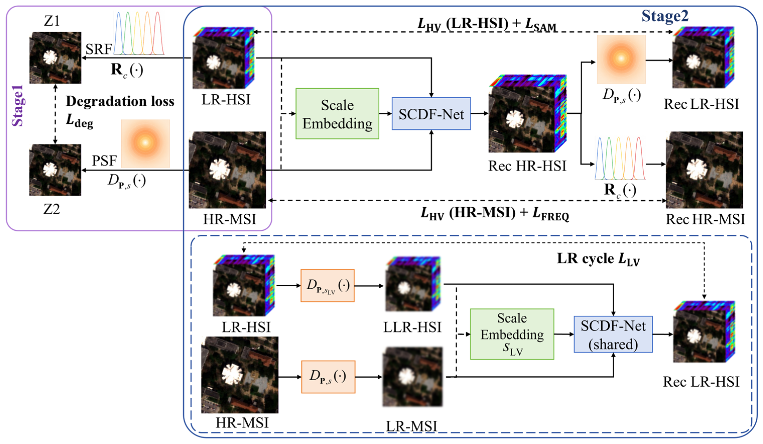
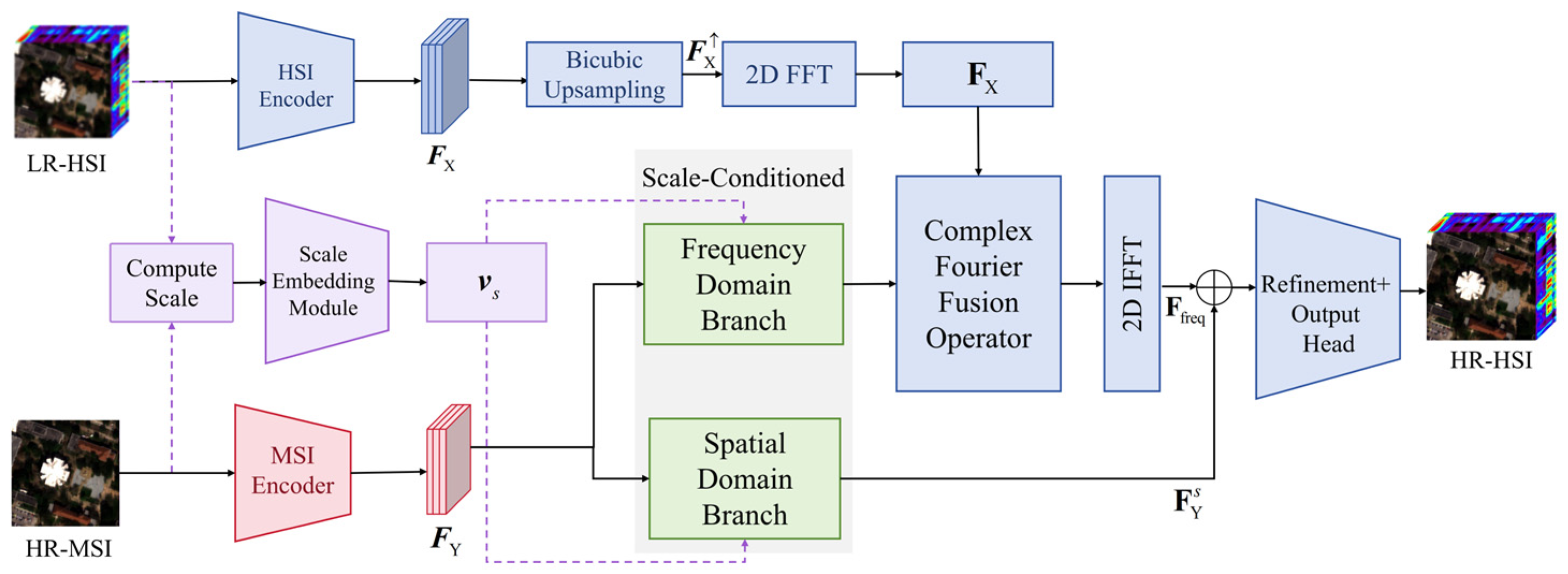
To address these challenges, we propose SCDF-Net, an unsupervised Scale-Conditioned Dual-domain Fusion Network that couples scale-controlled degradation alignment with frequency–spatial detail injection, supporting both integer and non-integer spatial resolution ratios. Here, dual-domain refers to the frequency-domain and spatial-domain feature pathways, which is distinct from the observation-domain consistency used for self-supervised training. The proposed method treats the spatial scale factor as a continuous conditioning variable. In the degradation estimation stage, the deterministic scale factor is used to define scale-controlled target-grid degradation, so that degraded observations are spatially aligned and comparable. In the fusion stage, the same scale factor is mapped into a learnable scale embedding vector to modulate frequency-domain and spatial-domain detail extraction. In this way, SCDF-Net can be applied to a given spatial resolution ratio—integer or fractional—directly on the native input grids, without resampling the inputs to an integer ratio and without requiring ground-truth HR-HSIs.

The main contributions of this work are summarized as follows:

(1)

We propose an unsupervised scale-conditioned HSI–MSI fusion framework that supports both integer and non-integer spatial resolution ratios. By introducing scale-controlled target-grid degradation and a scale embedding, the proposed method allows observation-domain constraints to be constructed on aligned grids under fractional scale factors.

(2)

We design a two-stage degradation-aware training strategy. The PSF and SRF are first estimated from the observed LR-HSI/HR-MSI pair in a self-supervised manner. The learned degradation operators are then frozen as physical priors to construct observation-domain constraints for unsupervised fusion training.

(3)

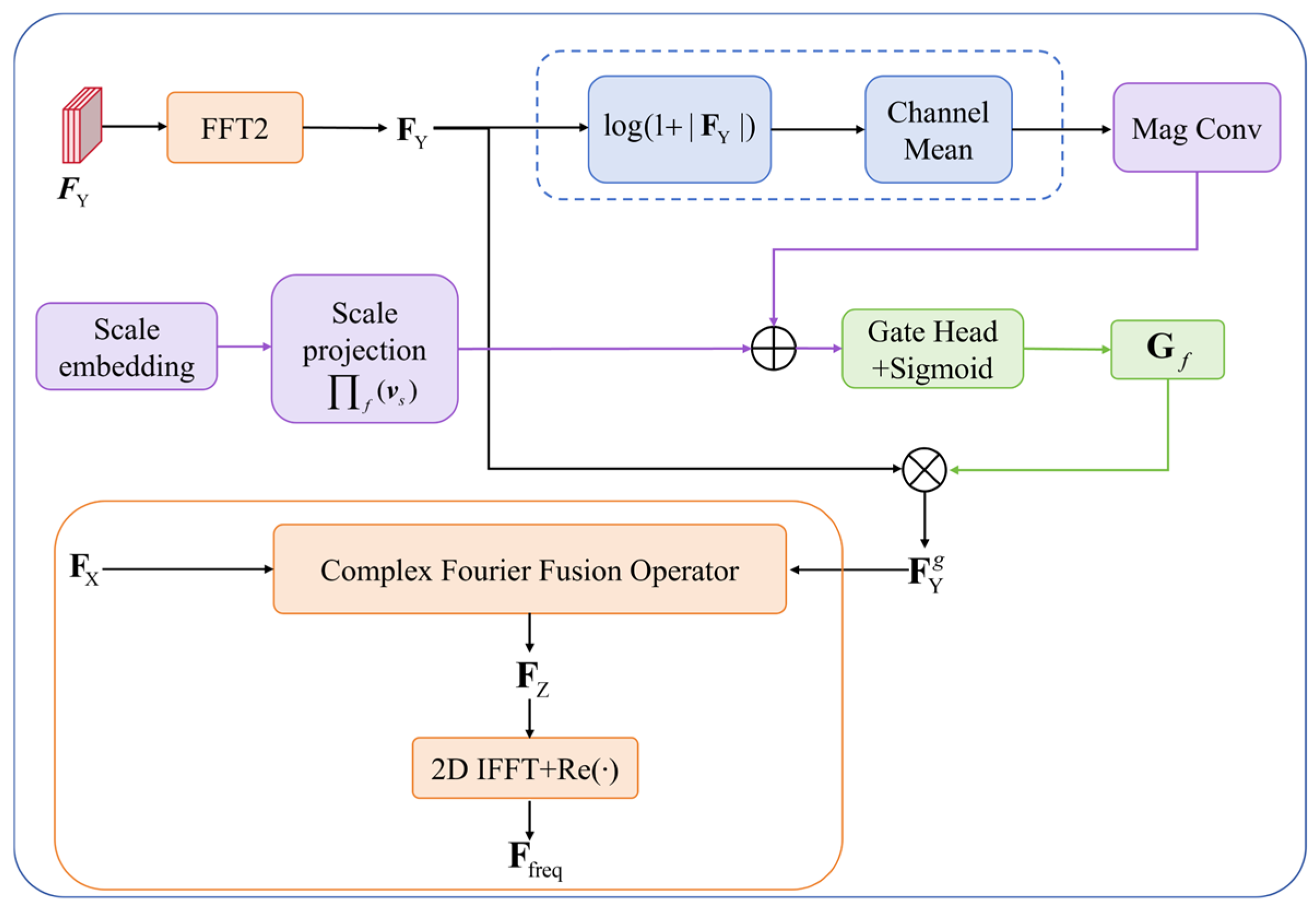
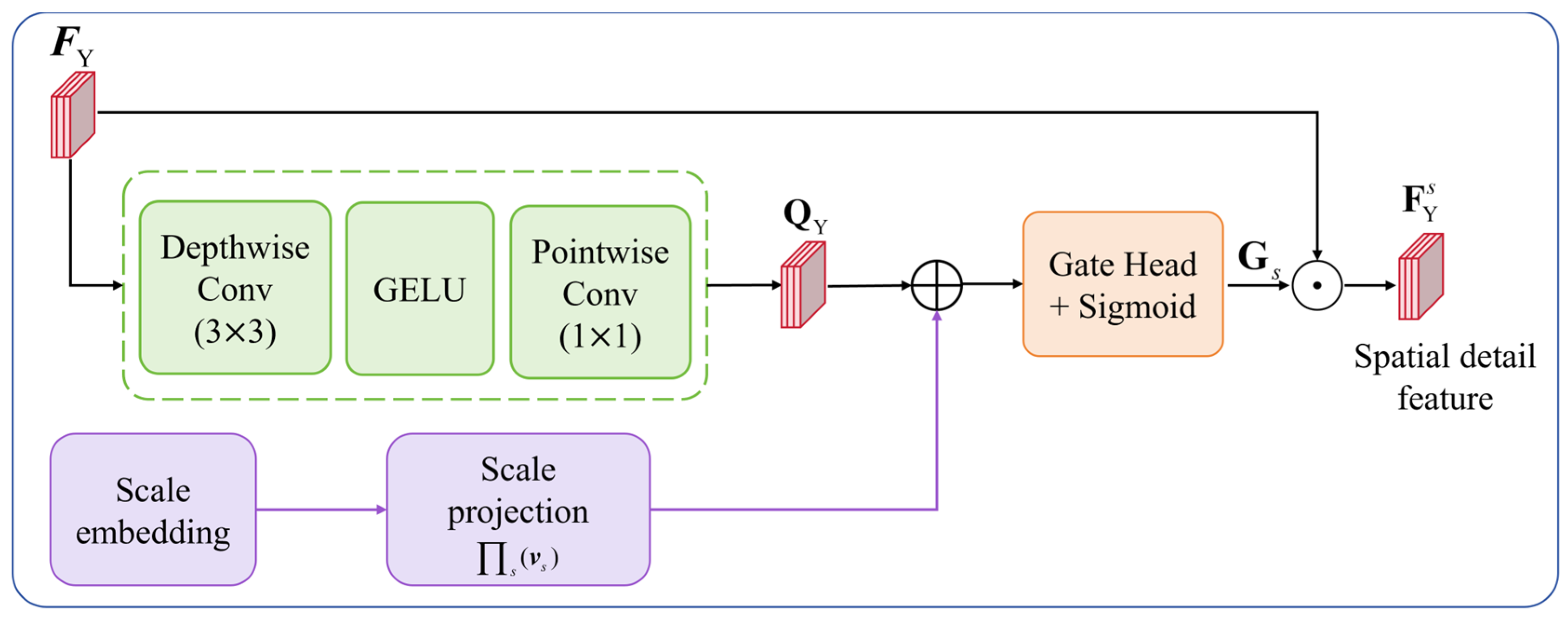
We develop a scale-conditioned frequency–spatial dual-domain fusion network. The frequency-domain branch enhances high-frequency spatial details from HR-MSIs, while the spatial-domain branch provides complementary structural information. Both branches are modulated by the scale embedding, enabling adaptive detail injection while preserving spectral fidelity.

2. Related Work

2.1. Traditional HSI–MSI Fusion Methods

Traditional HSI–MSI fusion methods usually reconstruct HR-HSIs by combining explicit observation models with handcrafted priors. According to existing surveys, these methods can be broadly grouped into component-substitution/detail-injection methods, spectral-unmixing or matrix-factorization methods, and optimization-based reconstruction methods [2,3,4].

In component-substitution and detail-injection methods, spatial information from high-resolution observations is injected into the upsampled hyperspectral image. Aiazzi et al. proposed the Gram–Schmidt Adaptive (GSA) method, which improves component substitution by using multivariate regression between multispectral and panchromatic-like components [8]. This type of method is efficient and easy to implement, but it may introduce spectral distortion when the assumed relationship between spatial and spectral components is inaccurate.

Spectral-unmixing and matrix-factorization methods describe the target HR-HSI using low-dimensional spectral and spatial factors. Yokoya et al. proposed coupled nonnegative matrix factorization (CNMF), which jointly factorizes LR-HSIs and HR-MSIs into endmembers and abundance maps [5]. Lanaras et al. further developed coupled spectral unmixing to estimate the shared spectral and spatial factors from the two modalities [9]. These methods provide clear physical interpretability, but their performance depends strongly on endmember estimation, linear mixing assumptions, and degradation-model accuracy.

Optimization-based methods formulate HSI–MSI fusion as an inverse problem with explicit priors and regularization. Simões et al. proposed HySure, which combines subspace representation, spatial-spectral degradation modeling, and total variation regularization [7]. Wei et al. introduced a sparse-representation-based fusion method that exploits spectral redundancy and spatial correlation through learned dictionaries [10]. These methods are more flexible than simple detail-injection approaches, but they often require reliable PSF/SRF information and careful parameter tuning.

Traditional methods are interpretable and do not require large-scale training data. However, they usually rely on fixed degradation assumptions or accurately known observation models, which limits their robustness under unknown degradation or non-integer spatial resolution ratios.

2.2. Supervised Deep Learning-Based HSI–MSI Fusion Methods

Supervised deep learning methods learn nonlinear spatial-spectral mappings from paired or simulated training data. Compared with traditional optimization-based methods, deep networks usually achieve stronger representation ability and better reconstruction performance when reliable HR-HSI references are available [14,15,16,17,18,19,20,21,22,23,24,25].

CNN-based methods first became a common solution for extracting complementary modality features. Yang et al. proposed a two-branch CNN that extracts spectral features from LR-HSIs and spatial features from HR-MSIs before fusion [15]. Palsson et al. introduced a 3D CNN-based fusion method to exploit local spectral–spatial correlations [14]. These CNN-based methods improve reconstruction quality, but they usually require paired HR-HSI labels and are trained under fixed degradation or scale settings.

Model-guided deep networks further embed physical observation models into trainable architectures. Xie et al. proposed MS/HS Fusion Net, which unfolds an optimization process into a deep network for HSI–MSI fusion [17]. They further developed MHF-Net, an interpretable proximal-gradient-unfolding network based on the linear observation model [18]. These methods improve interpretability and observation consistency, but they still depend on supervised training samples and predefined degradation assumptions.

Transformer-based methods have recently been introduced to model long-range spatial-spectral dependencies and cross-modal interactions. Jia et al. proposed MSST-Net, which uses multiscale spatial-spectral Transformer modeling to enhance feature representation [19]. Ma et al. proposed a reciprocal Transformer to strengthen bidirectional interaction between LR-HSI and HR-MSI features [20]. Although Transformer-based methods increase representation capacity, they often require large training sets, high computation, and fixed training configurations.

Supervised deep learning methods have strong reconstruction ability, but their dependence on paired HR-HSI references limits their applicability in real remote sensing scenarios. Their generalization ability is also restricted when the testing scale or degradation differs from the training setting.

2.3. Unsupervised Deep Learning-Based HSI–MSI Fusion Methods

Unsupervised and self-supervised HSI–MSI fusion methods reduce the dependence on ground-truth HR-HSIs by constructing supervision from the observed LR-HSI/HR-MSI pair. These methods usually degrade the reconstructed HR-HSI back to the observation domains and optimize the network through observation-domain consistency [26,27,28,29,30,31,32,33].

Degradation-aware unsupervised methods focus on learning or using spatial and spectral degradation models during training. Li et al. proposed UDALN, which estimates degradation processes with dedicated modules in a multi-stage unsupervised framework [26]. Li et al. further proposed UMC2FF, a model-guided coarse-to-fine fusion network that progressively refines the fused image through physical observation constraints [28]. These methods improve practical usability, but they still mainly work under predefined degradation and scale settings.

Other unsupervised methods address practical cross-sensor issues such as misregistration and modality alignment. Qu et al. proposed u2MDN, which introduces Mutual Dirichlet-Net to improve robustness under unregistered HSI–MSI inputs [27]. This method is useful for real-scene fusion, but its main focus is modality alignment rather than reconstruction under varying (including non-integer) scale ratios.

Recent continuous- and implicit-representation methods improve scale flexibility. Wang et al. proposed CLoRF, which uses continuous low-rank factorization to reconstruct fused images at user-specified resolutions [30]. Liang et al. proposed FeINFN, a Fourier-enhanced implicit neural fusion network that improves high-frequency reconstruction through spatial-frequency implicit modeling [31]. These methods show the importance of continuous scale modeling and frequency-domain information, but the joint modeling of scale-controlled degradation alignment, learned PSF/SRF priors, and scale-conditioned frequency–spatial detail injection remains insufficiently explored.

Overall, degradation-aware and alignment-oriented unsupervised methods mainly improve training practicality and robustness, whereas continuous- and implicit-representation-based methods further enhance resolution flexibility. However, degradation alignment under non-integer scales, adaptive detail injection, and spectral fidelity preservation remain insufficiently coupled. This motivates the proposed SCDF-Net framework, which uses learned degradation priors, continuous scale embedding, and scale-conditioned frequency- and spatial-domain fusion for unsupervised HSI–MSI reconstruction under integer and fractional scale factors.

3. Method

3.1. Overall Training Framework

Let ${\mathbf{X}}_{\mathrm{LR}}\in {\mathbb{R}}^{B\times h\times w}$ denote the observed low-spatial-resolution hyperspectral image (LR-HSI), and let ${\mathbf{Y}}_{\mathrm{HR}}\in {\mathbb{R}}^{C\times H\times W}$ denote the observed high-spatial-resolution multispectral image (HR-MSI), where $B$ and $C$ represent the numbers of hyperspectral and multispectral bands, respectively, and $C\ll B$. The objective of HSI–MSI fusion is to reconstruct a high-spatial-resolution hyperspectral image ${\widehat{\mathbf{X}}}_{\mathrm{HR}}\in {\mathbb{R}}^{B\times H\times W}$ [2,3,4].

The spatial scale factor is determined by the input spatial sizes:

$$\mathit{s} = [{\mathrm{s}}_{\mathrm{h}},{\mathrm{s}}_{\mathrm{w}}] = [\mathrm{H}/\mathrm{h}, \mathrm{W}/\mathrm{w}]$$

(1)

This scale factor is deterministic and is directly computed from the observed image sizes. Specifically, $\mathit{s}$ describes the vertical and horizontal resolution ratios between the HR-MSI and LR-HSI, and therefore provides an explicit scale condition for fusion under integer and fractional target ratios. In Stage 1, $\mathit{s}$ is used to define the scale-controlled spatial degradation and target-grid resampling process. In Stage 2, the same scale factor is further mapped into a learnable scale embedding vector to condition the fusion on the target ratio.

The proposed framework is trained in two consecutive stages, as shown in Figure 1. In Stage 1, a degradation model estimation module estimates the spatial point spread function (PSF) $\mathbf{P}$ and spectral response function (SRF) $\mathbf{R}$ from the available LR-HSI/HR-MSI pair. In Stage 2, the learned degradation operators are frozen and used as physical degradation priors to train the proposed SCDF-Net fusion network through self-supervised observation-domain consistency.

3.2. Stage 1: Degradation Model Estimation

The purpose of Stage 1 is to estimate the spatial and spectral degradation relationships between the two observed modalities. The SRF $\mathbf{R}$ maps the HSI spectral space to the MSI spectral space [3,5,7,11]. For the $c$-th multispectral band, the spectral degradation is written as

$${\mathit{Y}}_{\mathrm{c}}={ \mathit{R}}_{\mathrm{c}}(\mathit{X}), \mathrm{c} =1,\dots ,\mathrm{C}$$

(2)

where ${\mathbf{R}}_c(·)$ denotes the spectral response mapping from the HSI bands to the $c$-th MSI band. The SRF matrix $(\mathbf{R}\in {\mathbb{R}}^{C\times B})$ maps B hyperspectral bands to $C$ multispectral bands, and each row corresponds to the spectral response of one MSI band. The SRF weights are constrained to be nonnegative and normalized to preserve physical interpretability. In this work, the SRF is assumed to be spatially invariant, nonnegative, and row-normalized. The learned SRF is therefore used as an effective spectral degradation operator for self-supervised training.

The spatial degradation is modeled by a PSF-based blur-and-resampling operation [3,7,11,26]. The PSF describes local spatial blur, while the spatial size reduction is achieved by resampling the blurred image to the LR-HSI grid. The PSF is not assumed to perform downsampling alone; instead, the spatial size reduction is explicitly determined by the target-grid resampling operation. For an input image $\mathbf{Z}$, the spatial degradation is denoted as

$${\mathrm{D}}_{P,\mathbf{s}}(\mathrm{Z}) =S_{\mathit{s}} (\mathbf{P}*\mathbf{Z})$$

(3)

where $*$ denotes band-wise two-dimensional convolution, and $S_{\mathit{s}}(·)$ denotes scale-controlled resampling to the LR-HSI grid. The same blur-and-resampling formulation is used for both integer and non-integer scale factors. Because the same scale-controlled blur-and-resampling operator is used in both degradation estimation and fusion training, any interpolation effect under non-integer scale factors is modeled consistently by this shared operator, so the self-supervised observation-domain losses remain self-consistent across the two stages.

Based on the two degradation operators, the degradation model estimation module constructs two LR-MSI estimates on the LR-HSI grid:

$${\mathbf{Z}}_{1 }= \mathbf{R}\left({\mathbf{X}}_{\mathrm{LR}}), {\mathbf{Z}}_2 = D_{\mathbf{P},\mathbf{s}}\right({\mathbf{Y}}_{\mathrm{HR}})$$

(4)

The first path spectrally projects the LR-HSI into the MSI spectral space. The second path blurs the HR-MSI with the learned PSF and resamples it onto the LR-HSI grid. Therefore, both ${\mathbf{Z}}_1$ and ${\mathbf{Z}}_2$ are defined on the LR-HSI reference grid with the same size $C\times h\times w$, ensuring that the degradation alignment loss compares spatially aligned LR-MSI observations pixel by pixel. The degradation alignment loss is defined as:

$${\mathrm{L}}_{\mathit{deg}}={ ‖{\mathbf{Z}}_1 - {\mathbf{Z}}_2‖}_1$$

(5)

where $L_{\mathrm{deg}}$ denotes the degradation alignment loss used to train the degradation model estimation module in Stage 1. During optimization, the PSF and SRF are constrained to be nonnegative and normalized. After Stage 1, the learned PSF $\mathbf{P}$ and SRF $\mathbf{R}$ are fixed and transferred to Stage 2 as frozen degradation operators. The degradation estimation stage plays two important roles in the proposed framework. First, it provides a physically meaningful initialization of the spatial and spectral degradation relationships between the observed LR-HSI and HR-MSI, which alleviates the ill-posedness of the unsupervised fusion problem. Second, the estimated PSF and SRF serve as frozen degradation priors in Stage 2, enabling the construction of self-supervised observation-domain constraints that connect the reconstructed HR-HSI with the observed LR-HSI and HR-MSI. Without these priors, the network would lack explicit guidance on how the observed images are related to the target HR-HSI, making the unsupervised fusion task more challenging.

3.3. Stage 2: Unsupervised Fusion Network Training

In Stage 2, the PSF $\mathbf{P}$ and SRF $\mathbf{R}$ estimated in Stage 1 are fixed and used as physical degradation priors [26,28,29]. The reconstructed HR-HSI is constrained by two complementary observation-domain constraints, together with HSI-space spectral consistency and MSI-space frequency consistency. The two observation-domain constraints shown in Figure 1—main-reconstruction consistency $L_{\mathrm{HV}}$ and low-resolution cycle consistency $L_{\mathrm{LV}}$—provide complementary self-supervision: $L_{\mathrm{HV}}$ degrades the predicted HR-HSI to reproduce the observed LR-HSI and HR-MSI, whereas $L_{\mathrm{LV}}$ reconstructs the original LR-HSI from a further degraded LR-HSI/LR-MSI pair constructed at cycle ratios randomly sampled from a continuous range. We refer to these two terms jointly as dual observation-domain consistency. It is important to clarify that the term “dual” is used in two different contexts in this paper. The first refers to the two complementary observation-domain constraints ($L_{\mathrm{HV}}$ and $L_{\mathrm{LV}}$), which we collectively term “dual observation-domain consistency”. The second refers to the two feature-processing pathways in the network architecture, i.e., the frequency-domain and spatial-domain branches, which we term the “dual-domain network”. These two uses of “dual” denote different aspects of the framework and should not be confused. In parallel, the frequency- and spatial-domain branches form the dual-domain detail-modeling pathway; thus, dual observation-domain consistency and dual-domain detail modeling denote different components of the framework.

3.3.1. SCDF-Net

The overall architecture of SCDF-Net is illustrated in Figure 2. SCDF-Net takes the observed LR-HSI ${\mathbf{X}}_{\mathrm{LR}}$ and HR-MSI ${\mathbf{Y}}_{\mathrm{HR}}$ as inputs. The continuous scale vector $\mathit{s}$ defined in Equation (1) is first mapped into a learnable scale embedding ${\mathit{v}}_{\mathit{s}}$. Rather than being concatenated with the input images or encoder features, the scale embedding is projected into the frequency- and spatial-domain gates: the projection is reshaped and broadcast as a scale-conditioned bias map before gate generation, so that the gates are conditioned on the resolution gap of the current input. Although each model is trained for a single target ratio, the low-resolution cycle (Section 3.3.4) reconstructs ${\mathbf{X}}_{\mathrm{LR}}$ at cycle ratios randomly sampled from a continuous range, so the scale embedding is exposed to a continuous range of resolution gaps during training.

The scale embedding serves as a bridge between the target resolution ratio and the feature extraction process. Since different scale factors correspond to different degrees of spatial information loss, the network needs to know the current resolution gap to adjust its feature extraction accordingly. The scale embedding encodes this information and modulates the frequency- and spatial-domain gates, allowing the network to adapt its behavior to the specific scale setting. This design is particularly important for fractional scale factors, where the resolution gap cannot be represented by simple integer interpolation.

The dual-domain feature learning strategy is motivated by the complementary nature of frequency-domain and spatial-domain information. The frequency-domain branch is sensitive to global periodic patterns and high-frequency variations, which correspond to texture and edge structures in the image, while the spatial-domain branch captures local structural details that may be less prominent in the frequency representation. By combining these two pathways, the network can recover both global and local spatial structures, leading to improved reconstruction quality.

$${\mathit{v}}_{\mathit{s}}=\varphi (\mathit{s}), {\mathit{F}}_{\mathrm{X}}^{\uparrow }=U(E_X({\mathbf{X}}_{\mathrm{LR}});H,W), {\mathit{F}}_{\mathrm{Y}}={ E}_{\mathrm{Y}}({\mathbf{Y}}_{\mathrm{HR}})$$

(6)

Here, $\varphi (·)$ denotes the scale-embedding MLP, and $E_{\mathrm{X}}$ and $E_{\mathrm{Y}}$ denote the HSI encoder and MSI encoder, respectively. $U(·)$ denotes bicubic feature upsampling, which aligns the LR-HSI feature with the HR-MSI spatial grid before dual-domain fusion. The aligned HSI feature ${\mathit{F}}_{\mathrm{X}}^{\uparrow }$ provides the spectral foundation, while the MSI feature ${\mathit{F}}_{\mathrm{Y}}$ provides high-resolution spatial structures. In the following network description and figures, bold italic symbols denote the aligned encoder features supplied to the two branches, whereas bold upright symbols denote the intermediate and output tensors generated within the frequency- and spatial-domain branches.

After feature encoding and spatial alignment, ${\mathit{F}}_{\mathrm{X}}^{\uparrow }$ is transformed into the HSI spectrum ${\mathbf{F}}_{\mathrm{X}}$. In parallel, ${\mathit{F}}_{\mathrm{Y}}$ is processed by the scale-conditioned frequency-domain and spatial-domain branches. The frequency-domain branch generates the gated MSI spectrum ${\mathbf{F}}_{\mathrm{Y}}^g$, which is fused with ${\mathbf{F}}_{\mathrm{X}}$ and converted back to the spatial domain to obtain ${\mathbf{F}}_{\mathrm{freq}}$. The spatial-domain branch produces the scale-conditioned spatial detail feature ${\mathbf{F}}_{\mathrm{Y}}^s$. As illustrated in Figure 2, the frequency-fused feature and the spatial-detail feature are added and then passed through the refinement and output heads:

$${\widehat{\mathit{X}}}_{\mathrm{HR}} ={ H}_{\mathit{out}}\left(H_{\mathit{ref}}\left({\mathbf{F}}_{\mathrm{freq}}+{\mathit{F}}_Y^{\mathrm{s}}\right)\right)$$

(7)

Here, ${\mathbf{F}}_{\mathrm{freq}}$ denotes the frequency-fused spatial feature obtained after complex Fourier fusion and inverse Fourier transformation, and ${\mathbf{F}}_{\mathrm{Y}}^s$ denotes the scale-conditioned spatial detail feature produced by the spatial-domain branch. $H_{\mathit{ref}}(·)$ denotes the lightweight refinement module, and $H_{\mathit{out}}(·)$ maps the refined feature to the hyperspectral output space.

3.3.2. Frequency-Domain Branch

As illustrated in Figure 3, the frequency-domain branch transforms the MSI feature into the Fourier domain and generates a scale-conditioned gate from its magnitude response. The gate modulates the complete complex spectrum, thereby preserving both amplitude and phase information for subsequent fusion.

$${\mathbf{F}}_{\mathrm{X}}=\mathrm{FFT}({\mathit{F}}_{\mathrm{X}}^{\uparrow }), {\mathbf{F}}_{\mathrm{Y}}=\mathrm{FFT}({\mathit{F}}_{\mathrm{Y}}), {\mathbf{A}}_Y={\mathit{mean}}_c(\log (1+\left|{\mathbf{F}}_{\mathrm{Y}}\right|))$$

(8)

where $\mathrm{FFT}(·)$ denotes the two-dimensional Fourier transform, and ${\mathit{mean}}_c(·)$ denotes channel-wise averaging. Here, ${\mathbf{A}}_{\mathrm{Y}}$ is the channel-averaged magnitude descriptor of the MSI spectrum. It is computed only from the magnitude spectrum and is used for gate generation. The magnitude descriptor is not used to reconstruct the spectrum directly; it only provides a scale-conditioned gating cue, while the complete complex spectrum ${\mathbf{F}}_{\mathrm{Y}}$ is retained for subsequent modulation and fusion. The Fourier transform is adopted in the frequency-domain branch for two main reasons. First, it provides a global frequency representation that directly aligns with the frequency consistency loss defined in Equation (17), enabling efficient comparison of high-frequency components between the reconstructed and observed HR-MSI without introducing additional hyperparameters such as decomposition levels or wavelet bases. Second, the Fourier transform preserves phase information, which is critical for maintaining spatial structures when the modulated complex spectrum is transformed back to the spatial domain. Although wavelet transform offers multi-scale localization, it would increase the complexity of the branch and is not directly required for the proposed frequency consistency constraint. The magnitude descriptor and the scale embedding are jointly fed into a frequency gate generator to produce a scale-conditioned frequency gate:

$${\mathbf{G}}_f=\sigma (g_f ({\mathbf{A}}_{\mathrm{Y}},{\mathit{v}}_s)), {\mathbf{F}}_{\mathrm{Y}}^g={\mathbf{G}}_f \odot { \mathbf{F}}_{\mathrm{Y}}$$

(9)

where $g_f(·,·)$ denotes the scale-conditioned frequency gate mapping before sigmoid activation, $\sigma (·)$ denotes the sigmoid function, ${\mathbf{G}}_f$ denotes the resulting single-channel frequency gate, $\odot$ denotes element-wise multiplication, and ${\mathbf{F}}_{\mathrm{Y}}$ denotes the complete complex MSI spectrum. The gate ${\mathbf{G}}_f$ is broadcast across feature channels before modulation, so the complete spectrum, including its phase information, is retained.

After gate modulation, the scale-gated MSI spectrum ${\mathbf{F}}_{\mathrm{Y}}^g$ is combined with the spectrum ${\mathbf{F}}_{\mathrm{X}}$ of the spatially aligned HSI feature through a learnable complex Fourier fusion operator:

$${\mathbf{F}}_{\mathrm{Z}} = {\mathbf{F}}_{\mathrm{X}} + \alpha C_f({\mathbf{F}}_{\mathrm{X}}, {\mathbf{F}}_{\mathrm{Y}}^g) + (1-\alpha ){\mathbf{F}}_{\mathrm{Y}}^g, {\mathbf{F}}_{\mathrm{freq}} = \mathrm{Re}(\mathrm{IFFT}({\mathbf{F}}_{\mathrm{Z}}))$$

(10)

Here, ${\mathbf{F}}_{\mathrm{Z}}$ denotes the fused complex spectrum produced by the complex Fourier fusion operator. $C_f(·)$ predicts a complex residual correction from ${\mathbf{F}}_{\mathrm{X}}$ and ${\mathbf{F}}_{\mathrm{Y}}^g$, while the complete weighted combination in Equation (10) forms the complex Fourier fusion operation shown in Figure 3. IFFT(·) denotes the inverse Fourier transform, and Re(·) extracts the real component of the inverse-transformed feature. In practice, $C_f(·)$ is implemented by applying real-valued convolutions to the concatenated real and imaginary components of the two complex spectra. By operating on both real and imaginary components, $C_f(·)$ exploits amplitude- and phase-related information, so the fusion is not limited to magnitude enhancement. The coefficient α is a learnable scalar bounded in [0, 1], and ${\mathbf{F}}_{\mathrm{freq}}$ denotes the frequency-fused spatial feature after inverse Fourier transformation.

3.3.3. Spatial-Domain Branch

Figure 4 illustrates the scale-conditioned spatial-domain branch, which provides a complementary real-domain pathway for extracting edge- and texture-related local structures from the encoded MSI feature. It extracts a spatial-detail proxy from the MSI feature using depthwise and pointwise convolutions, and then uses the scale embedding to control the spatial gate. This branch extracts spatial details only from the MSI feature ${\mathit{F}}_{\mathrm{Y}}$, while the HSI branch mainly provides the spectral foundation through the main fusion pathway. The projected scale embedding is reshaped and broadcast to the spatial size of the MSI feature before being added to the spatial-detail proxy:

$${\mathbf{Q}}_{\mathrm{Y}}=W_p\delta (W_d({\mathit{F}}_Y)), {\mathbf{G}}_s=\sigma (g_s({\mathbf{Q}}_{\mathrm{Y}}+{\mathsf{\Pi }}_s({\mathit{v}}_s))), {\mathbf{F}}_{\mathrm{Y}}^s={\mathbf{G}}_s\odot {\mathbf{F}}_{\mathrm{Y}}$$

(11)

where ${\mathbf{Q}}_{\mathrm{Y}}$ denotes the spatial-detail proxy extracted from the encoded MSI feature. $W_d$ and $W_p$ denote the depthwise and pointwise convolution operators, respectively, and $\delta (·)$ denotes the GELU activation. ${\mathsf{\Pi }}_s(·)$ denotes the scale projection in the spatial-domain branch, while $g_s(·)$ denotes the spatial gate mapping before sigmoid activation. The resulting single-channel gate ${\mathbf{G}}_s$ is broadcast across feature channels and applied to the encoded MSI feature ${\mathit{F}}_{\mathrm{Y}}$. The output ${\mathbf{F}}_{\mathrm{Y}}^s$ therefore represents the scale-conditioned spatial-detail feature selected from the MSI feature.

The resulting spatial-detail feature ${\mathbf{F}}_{\mathrm{Y}}^s$ is added to the frequency-fused spatial feature ${\mathbf{F}}_{\mathrm{freq}}$ before being passed to the refinement module, as defined in Equation (7).

3.3.4. Loss Functions

Since HR-HSI ground truth is unavailable in Stage 2, SCDF-Net is trained using self-supervised losses constructed from the observed LR-HSI and HR-MSI [26,27,28,29]. The second-stage objective consists of four terms: low-resolution cycle loss, high-resolution observation-domain loss, HSI-space SAM loss, and MSI-space frequency loss.

For the main reconstruction branch, the network first estimates the HR-HSI:

$${\widehat{\mathbf{X}}}_{\mathrm{HR}}=f_{\theta }({\mathit{X}}_{\mathit{LR}},{\mathit{Y}}_{\mathit{HR}};\varphi (\mathit{s}))$$

(12)

where $f_{\theta }(·)$ denotes the SCDF-Net fusion network with learnable parameters θ. The reconstructed HR-HSI is then projected back to the observed LR-HSI and HR-MSI domains:

$${\widehat{\mathbf{X}}}_{\mathrm{LR}}=D_{\mathbf{P},\mathit{s}}({\widehat{\mathbf{X}}}_{\mathrm{HR}}), {\widehat{\mathbf{Y}}}_{\mathrm{HR}}=\mathbf{R}({\widehat{\mathbf{X}}}_{\mathrm{HR}})$$

(13)

Here, $D_{\mathbf{P},\mathit{s}}(·)$ denotes the frozen spatial degradation operator, including PSF blur and target-grid resampling, and $\mathbf{R}(·)$ denotes the frozen SRF-based spectral projection. The resulting ${\widehat{\mathbf{X}}}_{\mathrm{LR}}$ and ${\widehat{\mathbf{Y}}}_{\mathrm{HR}}$ are the simulated observations generated from the reconstructed HR-HSI.

The high-resolution observation-domain loss is defined as

$$L_{\mathrm{HV}}={‖{\widehat{\mathbf{X}}}_{\mathrm{LR}}-{\mathbf{X}}_{\mathrm{LR}}‖}_1+{‖{\widehat{\mathbf{Y}}}_{\mathrm{HR}}-{\mathbf{Y}}_{\mathrm{HR}}‖}_1$$

(14)

where $L_{\mathrm{HV}}$ denotes the high-resolution observation-domain loss, including the LR-HSI observation term and the HR-MSI observation term. To provide a direct self-supervised target, a low-resolution cycle is further introduced. At each training iteration, a cycle ratio ${\mathit{s}}_{\mathrm{LV}}$ is randomly sampled from a continuous scale range, with the upper bound adjusted according to the maximum scale factor used in the corresponding experiment. The observed LR-HSI is spatially downsampled by ${\mathit{s}}_{\mathrm{LV}}$ to obtain a lower-resolution HSI ${\mathit{X}}_{\mathrm{LLR}}$, while the HR-MSI is degraded to the LR-HSI grid (a factor of s) to obtain ${\mathbf{Y}}_{\mathrm{L}\mathrm{R}}$. Since ${\mathbf{Y}}_{\mathrm{L}\mathrm{R}}$ lies on the grid of size [h, w] and ${\mathbf{X}}_{\mathrm{LLR}}$ on the grid of size [$h/{\mathit{s}}_{\mathrm{LV}}, w/{\mathit{s}}_{\mathrm{LV}}$], the spatial ratio between the two cycle inputs is exactly ${\mathit{s}}_{\mathrm{LV}}$, which is the value passed to the scale embedding. The same SCDF-Net with shared parameters reconstructs ${\mathbf{X}}_{\mathrm{LR}}$ from this degraded pair:

$$L_{\mathrm{LV}}={‖f_{\theta }({\mathbf{X}}_{\mathrm{LLR}},{\mathbf{Y}}_{\mathrm{LR}};\varphi ({\mathit{s}}_{\mathrm{LV}}))-{\mathbf{X}}_{\mathrm{LR}}‖}_1$$

(15)

where $L_{\mathrm{L}\mathrm{V}}$ denotes the low-resolution cycle loss, and ${\mathit{s}}_{\mathrm{LV}}$ is the randomly sampled cycle scale drawn from $\mathrm{U}(1,s_{\max })$, where $s_{\max }$ is adjusted according to the maximum scale factor considered in the corresponding experiment. The original ${\mathbf{X}}_{\mathrm{LR}}$ serves as an available reconstruction target, providing direct self-supervision without requiring HR-HSI ground truth. Because ${\mathit{s}}_{\mathrm{LV}}$ varies continuously across iterations, the scale embedding is exposed to different resolution gaps around the target setting, even though each model is optimized for a specific target scale.

The HSI-space SAM loss is used to preserve spectral consistency in the LR-HSI observation space:

$$L_{\mathrm{SAM}}={\displaystyle \frac{1}{\mathit{hw}}}{\displaystyle {\sum }_{q=1}^{\mathit{hw}}}\mathrm{SAM}\left({\widehat{\mathit{x}}}_q, {\mathit{x}}_q\right)$$

(16)

where $\mathrm{SAM}(·)$ denotes the spectral angle between two spectral vectors, and ${\widehat{\mathit{x}}}_q$ and ${\mathit{x}}_q$ denote the reconstructed and observed LR-HSI spectral vectors at pixel $q$, respectively.

To enhance high-frequency spatial details, a frequency consistency loss is imposed in the MSI observation space [31]:

$${\mathrm{L}}_{\mathrm{FREQ}}={‖\mathbf{M}\odot (|\mathrm{FFT}({\widehat{\mathbf{Y}}}_{\mathrm{HR}})|-\left|\mathrm{FFT}({\mathbf{Y}}_{\mathrm{HR}})\right|)‖}_1$$

(17)

where $\mathbf{M}$ is a binary high-frequency mask that suppresses the central low-frequency region, and ${\widehat{\mathbf{Y}}}_{\mathrm{HR}}$ and ${\mathbf{Y}}_{\mathrm{HR}}$ denote the simulated and observed HR-MSI, respectively. The binary high-frequency mask M is constructed in the Fourier domain after centering the spectrum via fftshift. The central low-frequency region is masked out, while the surrounding high-frequency region is preserved. In our experiments, the size of the preserved high-frequency region is determined by a keep ratio of 0.15, as described in Section 4.2. The final training objective is

$$L =L_{\mathrm{LV}}+L_{\mathrm{HV}}+{ \lambda }_{\mathrm{SAM}}{L}_{\mathrm{SAM}}+{ \lambda }_{\mathrm{FREQ}}{L}_{\mathrm{FREQ}}$$

(18)

where ${\lambda }_{\mathrm{SAM}}$ and ${\lambda }_{\mathrm{FREQ}}$ are the weights of the HSI-space SAM loss and MSI-space frequency loss, respectively. The LV and HV losses are used with unit weights because they provide the main reconstruction constraints in the low-resolution cycle and observation domains.

The final objective combines the LV, HV, HSI-space SAM, and FREQ losses. These terms respectively constrain low-resolution self-supervision, high-resolution observation-domain reconstruction, HSI-space spectral preservation, and MSI-space high-frequency consistency. The LV and HV losses are assigned unit weights because they provide the primary observation-domain reconstruction constraints and directly connect the reconstructed HR-HSI with the available LR-HSI and HR-MSI observations. The HSI-space SAM loss and MSI-space frequency loss are used as auxiliary regularization terms; therefore, relatively small weights are adopted to improve spectral-angle consistency and high-frequency spatial consistency without dominating the main observation-domain objective. In our experiments, λ_SAM and λ_FREQ were both set to 0.01 according to preliminary convergence observations and the relative numerical magnitudes of different loss terms, which maintained stable optimization while keeping the auxiliary constraints effective.

The four loss terms are designed to address different aspects of the unsupervised fusion problem. $L_{\mathrm{LV}}$ and $L_{\mathrm{HV}}$ provide the main reconstruction constraints by enforcing consistency between the reconstructed HR-HSI and the observed LR-HSI/HR-MSI through the frozen degradation operators. $L_{\mathrm{SAM}}$ is introduced to preserve spectral fidelity, as high PSNR or low RMSE does not guarantee spectral consistency. By enforcing angular similarity between the reconstructed and observed LR-HSI spectra, $L_{\mathrm{SAM}}$ encourages the network to maintain the spectral relationships learned from the input. $L_{\mathrm{FREQ}}$ targets the recovery of high-frequency spatial details, which are often lost during reconstruction. By aligning the high-frequency components of the MSI spectra, $L_{\mathrm{FREQ}}$ encourages the network to preserve fine spatial structures. Together, these four losses jointly guide the network toward a solution that is both spectrally accurate and spatially detailed.

4. Experiments and Results

4.1. Datasets

Experiments were conducted on four widely used hyperspectral remote sensing datasets, including Pavia University (PaviaU) [38], Washington D.C. Mall (WADC) [39], University of Houston 2018 (Houston18) [40], and Chikusei [41]. These datasets contain diverse land-cover types, spatial structures, and spectral characteristics, and therefore allow us to evaluate the fusion performance and robustness of HSI–MSI fusion methods across different scenes and spatial resolution ratios.

Since real paired LR-HSI, HR-MSI, and HR-HSI observations are difficult to obtain, the experiments were conducted following Wald’s protocol [42]. Specifically, the original HSI was regarded as the reference HR-HSI. The LR-HSI was generated by applying spatial degradation to the reference HR-HSI, including PSF-based spatial blurring and scale-controlled downsampling. The HR-MSI was generated by applying spectral degradation to the reference HR-HSI using the SRF. In this way, the reconstructed HR-HSI can be quantitatively compared with the reference image. Since both the LR-HSI and HR-MSI were simulated from the same reference HR-HSI, their spatial correspondence was maintained under the predefined target grids.

The PaviaU dataset captures an urban scene and contains 103 spectral bands ranging from 430 nm to 860 nm. The WADC dataset was acquired by the HYDICE sensor and contains 191 spectral bands covering approximately 400 nm to 2400 nm. The Houston18 dataset used in this study was derived from the 2018 IEEE GRSS Data Fusion Contest. The original hyperspectral data contain 48 spectral bands covering 380–1050 nm with a 1 m ground sampling distance. After removing unusable or noisy bands during preprocessing, 46 bands ranging from 389 nm to 1033 nm were retained in our experiments. The Chikusei dataset covers urban and agricultural areas and contains 128 spectral bands ranging from 363 nm to 1018 nm.

All images were normalized to the range [0, 1] band by band before training and testing. The input LR-HSI/HR-MSI pairs were spatially aligned before fusion. Unlike patch-based training strategies, the proposed method directly used the whole LR-HSI/HR-MSI image pair as input, without random cropping, sliding-window inference, or patch stitching. This whole-image setting avoids additional patch boundary effects and preserves the spatial correspondence between the input observations and the reconstructed HR-HSI.

4.2. Implementation Details

All experiments were implemented in PyTorch 2.0.0, with Python 3.8 and CUDA 11.8, and conducted on a workstation equipped with an NVIDIA GeForce RTX 4090D GPU. The proposed SCDF-Net was trained in an unsupervised manner without using ground-truth HR-HSI supervision. For each dataset and scale factor, the LR-HSI and HR-MSI inputs were generated following the degradation protocol described in Section 3. The same degradation strategy was applied to all compared methods to ensure consistent input conditions and fair evaluation under different scale settings.

The training process followed the two-stage optimization framework introduced in Section 3. In Stage 1, the degradation operators, including the PSF and SRF, were estimated from the observed LR-HSI/HR-MSI pairs. In Stage 2, the learned degradation operators were fixed and used as physical priors to construct self-supervised constraints for optimizing SCDF-Net. For different target scales, the degradation settings were adjusted according to the predefined scale factors. The learned PSF kernels were constrained to be nonnegative and normalized to unit sum before being used for spatial degradation, ensuring the physical consistency of the simulated observations.

To achieve arbitrary-scale fusion, the scale factor was represented as a continuous two-dimensional vector $\mathit{s} = [H/h,W/w]$, where H and W denote the spatial dimensions of the HR-MSI, and h and w represent those of the LR-HSI. The scale vector was mapped into a learnable scale embedding, which was subsequently used to condition the frequency-domain and spatial-domain gates. Before feature fusion, the LR-HSI feature was upsampled to the HR-MSI resolution to achieve spatial alignment between heterogeneous observations.

For optimization, the Adam optimizer was adopted with ${\beta }_1 = 0.5$ and ${\beta }_2 = 0.999$ [43]. The initial learning rate was set to $1 \times 10^{-4}$, and the number of training epochs was set to 10,000. Since the LR-HSI and HR-MSI observations were spatially aligned through the degradation-based simulation process, whole-image training was adopted instead of patch-based training. The batch size was set to 1 to preserve the complete spatial correspondence between the input observations and the self-supervised degradation constraints.

Following the loss definitions in Section 3, the low-resolution cycle constraint and the high-resolution observation-domain constraint were implemented using L1 reconstruction losses. During training, the low-resolution cycle ratio $s_{\mathrm{LV}}$ was randomly sampled from a continuous scale range, with the upper bound adjusted according to the maximum scale factor used in the corresponding experiment. The HSI-space SAM loss and MSI-space frequency consistency loss were weighted by ${\lambda }_{\mathit{SAM}} = 0.01$ and ${\lambda }_{\mathit{FREQ}} = 0.01$, respectively. These weights were empirically determined based on convergence behavior and validation performance. Meanwhile, the relative magnitudes of different loss terms were considered to maintain comparable gradient contributions during optimization and avoid domination by any single constraint. The high-frequency preservation ratio in the frequency consistency loss was set to 0.15.

For a fair comparison, all baseline methods were evaluated using the same simulated LR-HSI and HR-MSI inputs, normalization strategy, degradation settings, and evaluation metrics. For methods originally designed for fixed integer scale factors, the input observations were adapted to the target scale through interpolation-based resampling when necessary, and the models were retrained or re-executed under the corresponding scale settings. For UMC2FF, the available implementation was adopted and trained following the recommended settings as closely as possible. The input generation protocol, normalization strategy, and evaluation criteria were kept consistent with those used for SCDF-Net and other compared methods.

We further evaluated the computational complexity and efficiency of SCDF-Net in terms of the number of trainable parameters, training time, and inference time. SCDF-Net contains approximately 3.1 M trainable parameters. On an NVIDIA GeForce RTX 4090D GPU, the average training time is approximately 0.5 h for 10,000 epochs. Since the benchmark datasets have different spatial resolutions and image sizes, the average inference time over all four datasets is approximately 1.0 s per image (batch size = 1). For the efficiency comparison reported in

Table 1. Efficiency comparison of different deep learning-based methods on the same hardware.

Method	Parameters (M)	Inference Time (s)
UDALN	0.0023	0.0004
UMC2FF	0.0056	0.0029
u2MDN	0.0066	0.1383
CLoRF	1.42	0.0075
SCDF-Net	3.1	0.0071

, the inference time of all deep learning-based methods was measured on the Houston18 dataset under the same hardware environment and identical input setting, yielding an inference time of 0.0071 s per image for SCDF-Net. The frequency-domain branch mainly uses FFT-based transformation and lightweight gate generation, while the spatial-domain branch is implemented with depthwise and pointwise convolutions. Therefore, the additional computational cost introduced by the dual-domain branches remains moderate.

4.3. Evaluation Metrics

Quantitative performance was evaluated using five metrics: peak signal-to-noise ratio (PSNR), root mean square error (RMSE), spectral angle mapper (SAM), relative dimensionless global error in synthesis (ERGAS), and correlation coefficient (CC) [2,3,4,27,30]. PSNR and RMSE measure absolute reconstruction accuracy, ERGAS evaluates band-normalized global relative error, CC measures band-wise correlation, whereas SAM evaluates spectral fidelity.

For the reconstructed HR-HSI ${\widehat{\mathbf{X}}}_{\mathrm{HR}}$ and reference HR-HSI ${\mathbf{X}}_{\mathrm{HR}}$, PSNR, RMSE, and ERGAS are computed as

$$\mathrm{PSNR} =10{\log }_{10}({\displaystyle \frac{{\mathit{BHWL}}^2}{{\Vert {\widehat{\mathbf{X}}}_{\mathrm{HR}}-{\mathbf{X}}_{\mathrm{HR}}\Vert }_{\mathrm{F}}^2}})$$

(19)

$$\mathrm{RMSE}={\displaystyle \frac{{\Vert {\widehat{\mathbf{X}}}_{\mathrm{HR}}-{\mathbf{X}}_{\mathrm{HR}}\Vert }_{\mathrm{F}}}{\sqrt{\mathit{BHW}}}}$$

(20)

where B is the number of spectral bands, $H\times W$ is the spatial size, $L = 1$ is the maximum pixel value after normalization, and ${\Vert \Vert }_{\mathrm{F}}$ denotes the Frobenius norm.

$$\mathrm{ERGAS}={\displaystyle \frac{100}{r}}\sqrt{{\displaystyle \frac{1}{B}}{\displaystyle {\sum }_{b=1}^B}{\left({\displaystyle \frac{{\mathrm{RMSE}}_b}{{\mu }_b}}\right)}^2}$$

(21)

where $r$ denotes the spatial scale factor, ${\mathrm{RMSE}}_b$ is the RMSE of the b-th spectral band, and ${\mu }_b$ is the mean value of the b-th band in the reference HR-HSI. ERGAS measures the global relative reconstruction error after band-wise normalization, and lower ERGAS values indicate better overall fidelity.

$$\mathrm{CC}={\displaystyle \frac{1}{B}}{\displaystyle {\sum }_{\mathrm{b}=1}^B}\frac{{\displaystyle {\sum }_{i=1}^{\mathit{HW}}}\left({\widehat{x}}_{I,b}-{\overline{\widehat{x}}}_b\right)\left(x_{I,b}-{\overline{x}}_b\right)}{\sqrt{{\displaystyle {\sum }_{i=1}^{\mathit{HW}}}{\left({\widehat{x}}_{I,b}-{\overline{\widehat{x}}}_b\right)}^2}\sqrt{{\displaystyle {\sum }_{i=1}^{\mathit{HW}}}{\left(x_{I,b}-{\overline{x}}_b\right)}^2}}$$

(22)

where ${\overline{x}}_{I,b}$ and $x_{I,b}$ denote the reconstructed and reference pixel values at spatial pixel i and spectral band b, respectively. ${\overline{\widehat{x}}}_b \mathrm{and} {\overline{x}}_b$ are the mean values of the reconstructed and reference images in the $b$-th spectral band. CC measures the band-wise linear correlation between the reconstructed and reference HR-HSI, and the final value is averaged over all spectral bands. Higher CC values indicate better reconstruction performance.

SAM is obtained by averaging the spectral angle over all spatial pixels:

$$\mathrm{SAM}={\displaystyle \frac{1}{N}}{\sum }_{i=1}^N\arccos \left({\displaystyle \frac{{\widehat{x}}_i^{\mathrm{T}}{x}_i}{{‖{\widehat{x}}_i‖}_2{‖x_i‖}_2+\epsilon }}\right), N=\mathit{HW}$$

(23)

where ${\widehat{\mathit{x}}}_I$ and ${\mathit{x}}_I$ are the reconstructed and reference spectral vectors at pixel $i$, respectively, and $\epsilon$ is a small constant for numerical stability. The resulting mean spectral angle is converted from radians to degrees for reporting. Higher PSNR, CC and lower RMSE, ERGAS, and SAM values indicate better reconstruction performance.

Residual, MRAE, and SAM maps were additionally used for visual evaluation [27,30]. The pixel-wise MRAE map is defined as

$${\mathrm{MRAE}}_i={\displaystyle \frac{1}{B}}{\sum }_{b=1}^B{\displaystyle \frac{\left|{\widehat{x}}_{I,b}-x_{I,b}\right|}{\left|x_{I,b}\right|+\epsilon }}$$

(24)

where i and $b$ index the spatial pixels and spectral bands, respectively. The residual map shows absolute reconstruction errors, whereas the MRAE and SAM maps visualize the spatial distributions of relative errors and spectral distortion, respectively. These maps are used only for qualitative comparison and are not reported as scalar metrics.

4.4. Performance of Different Datasets at Different Scales

To evaluate the performance of SCDF-Net under different target scale factors, experiments were conducted under multiple spatial scale factors, including both integer and fractional ratios. Table 2 and Table 3 report the quantitative results on PaviaU, WADC, Houston18, and Chikusei.

As shown in Table 2 and Table 3, the reconstruction performance generally decreases as the scale factor increases. This is reasonable because larger scale factors lead to more severe spatial information loss in LR-HSIs and make HR-HSI reconstruction more challenging. Nevertheless, SCDF-Net maintains stable performance across all datasets. In particular, the results at fractional scale factors, such as ×1.5, ×2.4, and ×3.6, demonstrate that the proposed method can effectively handle non-integer spatial resolution ratios.

The performance differences among datasets are related to their scene complexity, spatial structure, and spectral variability. For example, WADC and Chikusei obtain relatively high PSNR values, while Houston18 presents a more challenging urban scene with complex spatial patterns. Overall, the multi-scale results verify that the proposed scale-controlled degradation and continuous scale embedding improve the adaptability of SCDF-Net under both integer and fractional scale factors. Notably, SCDF-Net is also evaluated at larger scale factors, including ×5.0 and ×6.0, which further examines its stability under more severe spatial information loss.

Table 2. Quantitative evaluation of SCDF-Net on PaviaU and WADC under different scale factors.

Scales	PaviaU					WADC
	PSNR	SAM	RMSE	ERGAS	CC	PSNR	SAM	RMSE	ERGAS	CC
1.5	42.8595	2.4203	0.0072	4.4895	0.9926	51.1957	1.3598	0.0028	4.0484	0.9791
2.0	42.0787	2.4765	0.0079	3.5209	0.9921	48.9587	1.7307	0.0036	2.4797	0.9732
2.4	40.4373	2.7202	0.0095	2.0629	0.9912	47.5650	1.9484	0.0042	2.5664	0.9724
3.0	39.7733	2.8447	0.0103	2.6284	0.9899	47.5159	2.0685	0.0042	1.8984	0.9705
3.6	39.2749	2.9415	0.0109	2.2333	0.9894	46.2245	2.4759	0.0049	1.8435	0.9677
4.0	38.9511	3.0169	0.0113	1.6421	0.9889	45.4189	2.7139	0.0054	1.5319	0.9623
5.0	38.7018	3.1930	0.0116	1.4774	0.9876	44.9716	3.2494	0.0056	1.6852	0.9567
6.0	38.5885	3.2736	0.0118	1.2410	0.9864	44.7558	3.3291	0.0058	1.4276	0.9538

Table 2. Quantitative evaluation of SCDF-Net on PaviaU and WADC under different scale factors.

Scales	PaviaU					WADC
	PSNR	SAM	RMSE	ERGAS	CC	PSNR	SAM	RMSE	ERGAS	CC
1.5	42.8595	2.4203	0.0072	4.4895	0.9926	51.1957	1.3598	0.0028	4.0484	0.9791
2.0	42.0787	2.4765	0.0079	3.5209	0.9921	48.9587	1.7307	0.0036	2.4797	0.9732
2.4	40.4373	2.7202	0.0095	2.0629	0.9912	47.5650	1.9484	0.0042	2.5664	0.9724
3.0	39.7733	2.8447	0.0103	2.6284	0.9899	47.5159	2.0685	0.0042	1.8984	0.9705
3.6	39.2749	2.9415	0.0109	2.2333	0.9894	46.2245	2.4759	0.0049	1.8435	0.9677
4.0	38.9511	3.0169	0.0113	1.6421	0.9889	45.4189	2.7139	0.0054	1.5319	0.9623
5.0	38.7018	3.1930	0.0116	1.4774	0.9876	44.9716	3.2494	0.0056	1.6852	0.9567
6.0	38.5885	3.2736	0.0118	1.2410	0.9864	44.7558	3.3291	0.0058	1.4276	0.9538

Table 3. Quantitative evaluation of SCDF-Net on Houston18 and Chikusei under different scale factors.

Scales	Houston18					Chikusei
	PSNR	SAM	RMSE	ERGAS	CC	PSNR	SAM	RMSE	ERGAS	CC
1.5	46.4720	1.2504	0.0047	2.3633	0.9983	50.9084	1.1025	0.0028	7.0201	0.9853
2.0	45.2481	1.3093	0.0055	1.8289	0.9989	50.1400	1.1215	0.0031	4.9887	0.9851
2.4	43.4804	1.3811	0.0067	1.7708	0.9979	49.1500	1.1499	0.0035	4.1706	0.9850
3.0	43.4472	1.4695	0.0067	1.5983	0.9977	48.7200	1.2345	0.0037	3.4455	0.9842
3.6	41.5300	1.6892	0.0084	1.6343	0.9971	48.6500	1.2847	0.0037	2.9132	0.9842
4.0	41.3550	1.6957	0.0086	1.5555	0.9957	47.6500	1.3870	0.0041	2.8290	0.9813
5.0	39.6708	2.2564	0.0104	1.3831	0.9937	45.1374	1.8166	0.0055	2.2933	0.9792
6.0	37.8763	2.8700	0.0128	1.6660	0.9910	44.0339	1.9414	0.0063	2.0369	0.9758

Table 3. Quantitative evaluation of SCDF-Net on Houston18 and Chikusei under different scale factors.

Scales	Houston18					Chikusei
	PSNR	SAM	RMSE	ERGAS	CC	PSNR	SAM	RMSE	ERGAS	CC
1.5	46.4720	1.2504	0.0047	2.3633	0.9983	50.9084	1.1025	0.0028	7.0201	0.9853
2.0	45.2481	1.3093	0.0055	1.8289	0.9989	50.1400	1.1215	0.0031	4.9887	0.9851
2.4	43.4804	1.3811	0.0067	1.7708	0.9979	49.1500	1.1499	0.0035	4.1706	0.9850
3.0	43.4472	1.4695	0.0067	1.5983	0.9977	48.7200	1.2345	0.0037	3.4455	0.9842
3.6	41.5300	1.6892	0.0084	1.6343	0.9971	48.6500	1.2847	0.0037	2.9132	0.9842
4.0	41.3550	1.6957	0.0086	1.5555	0.9957	47.6500	1.3870	0.0041	2.8290	0.9813
5.0	39.6708	2.2564	0.0104	1.3831	0.9937	45.1374	1.8166	0.0055	2.2933	0.9792
6.0	37.8763	2.8700	0.0128	1.6660	0.9910	44.0339	1.9414	0.0063	2.0369	0.9758

4.5. Baseline Comparison

For a fair comparison under different scale factors, all baseline methods were independently retrained or re-run for each target scale factor using the same simulated LR-HSI and HR-MSI inputs. Specifically, the LR-HSI was generated by the same PSF-based spatial degradation and target-grid resampling protocol, while the HR-MSI was generated using the same SRF-based spectral degradation. The training and testing data, normalization strategy, degradation setting, and evaluation metrics were kept identical for all methods. For methods originally designed for fixed integer scales, the input image pairs were regenerated on the corresponding target grid, and the model was retrained or re-executed under each scale setting. Fixed integer-ratio baselines cannot operate under ×2.4 directly, so they were adapted by interpolation-based resampling before training/testing, following the standard workaround for such methods. This adaptation may introduce additional approximation error; therefore, the ×2.4 comparison is interpreted as a practical comparison between fixed-scale adaptation and the proposed native fractional-scale fusion. All outputs were evaluated on the same HR-HSI grid with identical metrics. For learning-based baseline methods, we used the publicly available implementations when available and followed their recommended training settings. All baselines were trained or re-run under the same degradation setting and evaluation protocol, and the reported results were obtained after convergence.

Before comparing different fusion methods, we further analyze the degradation operators estimated in Stage 1, because the learned PSF and SRF are frozen and used as physical priors in Stage 2. Under Wald’s protocol, the spatial degradation kernel is predefined during data generation, which allows us to compare the estimated PSF with the reference PSF. Specifically, both kernels are normalized to unit sum, and the mean squared error (MSE) between them is computed. Under the ×2.4 scale setting, the PSF MSE values are 0.000059, 0.000041, 0.000123, and 0.000109 on PaviaU, WADC, Houston18, and Chikusei, respectively. These small errors indicate that Stage 1 can reliably recover the spatial degradation patterns across different scenes.

For the SRF, direct element-wise comparison is less straightforward because the learned spectral mapping and the simulated spectral response may use different parameterizations. Therefore, we evaluate its effect through observation-domain reconstruction consistency: the LR-HSI projected by the learned SRF should be consistent with the MSI observation after spectral degradation. Together, the low PSF estimation error and the observation-domain reconstruction consistency support the use of the learned PSF/SRF as frozen degradation priors in Stage 2.

We compared SCDF-Net with representative traditional and deep learning-based HSI–MSI fusion methods. The traditional methods include GSA [8], CNMF [5], and HySure [7], while the deep learning-based methods include CLoRF [30], UDALN [26], u2MDN [27], and UMC2FF [28]. The quantitative comparison results are reported in Table 3, Table 4, Table 5, Table 6, Table 7, Table 8, Table 9 and Table 10. In all quantitative comparison tables, bold and underlined values indicate the best and second-best results, respectively. In addition to PSNR, SAM, and RMSE, ERGAS and CC are also considered to evaluate band-normalized global error and spectral correlation, respectively. Overall, traditional methods generally show lower performance than deep learning-based methods because they rely on handcrafted priors, linear mixture assumptions, or fixed degradation models. These assumptions limit their flexibility when the spatial resolution ratio changes, especially under fractional and large-scale settings.

4.5.1. Comparison at Scale Factor ×1.5

Table 4 and Table 5 present the quantitative results at scale factor ×1.5, which is a fractional scale setting where fixed-integer methods require interpolation-based input adaptation. Traditional methods show limited performance, as their handcrafted priors and fixed degradation assumptions are insufficient to handle complex spatial–spectral relationships under non-integer scales. Deep learning-based methods generally achieve better reconstruction quality. Among them, UMC2FF achieves relatively strong results, particularly on Houston18 and Chikusei. SCDF-Net reports the highest PSNR and lowest SAM on all four datasets. Compared with the strongest PSNR baseline in each dataset, SCDF-Net improves PSNR by 1.2369 dB on PaviaU, 9.3838 dB on WADC, 1.4069 dB on Houston18, and 2.1754 dB on Chikusei. For ERGAS and CC, SCDF-Net remains close to the strongest results on most datasets, while some baselines obtain lower ERGAS or higher CC on individual datasets. The consistent improvements indicate that operating directly on the native fractional grid, rather than resampling to an integer ratio, is beneficial for fractional-scale fusion.

Table 4. Quantitative comparison on PaviaU and WADC at scale factor ×1.5.

Methods	PaviaU					WADC
	PSNR	SAM	RMSE	ERGAS	CC	PSNR	SAM	RMSE	ERGAS	CC
GSA	33.9090	4.0529	0.0202	7.7390	0.9789	36.8455	3.4489	0.0143	5.5495	0.9748
HySure	28.0279	5.5687	0.0397	13.6839	0.9153	31.4305	5.2443	0.0268	10.9401	0.8260
CNMF	37.3174	3.5195	0.0136	6.3228	0.9747	35.6997	2.3895	0.0164	4.3682	0.9699
CLoRF	37.1171	3.5006	0.0139	5.9111	0.9879	36.6413	3.7888	0.0147	8.1587	0.8884
UDALN	37.5061	3.3982	0.0133	6.1141	0.9863	35.9871	2.0385	0.0159	3.8989	0.9640
u2MDN	39.1697	2.9362	0.0110	4.7551	0.9911	41.8119	3.0819	0.0081	8.5111	0.9479
UMC2FF	41.6226	2.9570	0.0083	4.5847	0.9906	40.0802	1.5539	0.0099	2.5525	0.9605
Proposed	42.8595	2.4203	0.0072	4.4895	0.9926	51.1957	1.3598	0.0028	4.0484	0.9791

Note: Bold and underlined values denote the best and second-best results, respectively.

Table 4. Quantitative comparison on PaviaU and WADC at scale factor ×1.5.

Methods	PaviaU					WADC
	PSNR	SAM	RMSE	ERGAS	CC	PSNR	SAM	RMSE	ERGAS	CC
GSA	33.9090	4.0529	0.0202	7.7390	0.9789	36.8455	3.4489	0.0143	5.5495	0.9748
HySure	28.0279	5.5687	0.0397	13.6839	0.9153	31.4305	5.2443	0.0268	10.9401	0.8260
CNMF	37.3174	3.5195	0.0136	6.3228	0.9747	35.6997	2.3895	0.0164	4.3682	0.9699
CLoRF	37.1171	3.5006	0.0139	5.9111	0.9879	36.6413	3.7888	0.0147	8.1587	0.8884
UDALN	37.5061	3.3982	0.0133	6.1141	0.9863	35.9871	2.0385	0.0159	3.8989	0.9640
u2MDN	39.1697	2.9362	0.0110	4.7551	0.9911	41.8119	3.0819	0.0081	8.5111	0.9479
UMC2FF	41.6226	2.9570	0.0083	4.5847	0.9906	40.0802	1.5539	0.0099	2.5525	0.9605
Proposed	42.8595	2.4203	0.0072	4.4895	0.9926	51.1957	1.3598	0.0028	4.0484	0.9791

Note: Bold and underlined values denote the best and second-best results, respectively.

Table 5. Quantitative comparison on Houston18 and Chikusei at scale factor ×1.5.

Methods	Houston18					Chikusei
	PSNR	SAM	RMSE	ERGAS	CC	PSNR	SAM	RMSE	ERGAS	CC
GSA	40.7831	1.6827	0.0091	3.7098	0.9960	40.3523	1.5981	0.0096	5.7361	0.9829
HySure	33.7199	2.6260	0.0206	8.3985	0.9785	48.7330	2.7249	0.0037	12.7047	0.9199
CNMF	37.8003	3.2614	0.0129	6.4163	0.9811	43.5613	1.6538	0.0066	7.1234	0.9493
CLoRF	41.2973	2.1842	0.0086	3.7040	0.9954	45.2046	1.6904	0.0055	8.4697	0.9747
UDALN	39.4220	2.0005	0.0107	3.2957	0.9977	36.3732	3.2918	0.0152	13.0614	0.9677
u2MDN	43.3015	1.8552	0.0068	2.9299	0.9977	46.2334	3.4849	0.0049	7.1300	0.9831
UMC2FF	45.0651	1.7757	0.0056	2.3510	0.9980	46.9108	1.6727	0.0044	6.6978	0.9827
Proposed	46.4720	1.2504	0.0047	2.3633	0.9983	50.9084	1.1025	0.0028	7.0201	0.9853

Note: Bold and underlined values denote the best and second-best results, respectively.

Table 5. Quantitative comparison on Houston18 and Chikusei at scale factor ×1.5.

Methods	Houston18					Chikusei
	PSNR	SAM	RMSE	ERGAS	CC	PSNR	SAM	RMSE	ERGAS	CC
GSA	40.7831	1.6827	0.0091	3.7098	0.9960	40.3523	1.5981	0.0096	5.7361	0.9829
HySure	33.7199	2.6260	0.0206	8.3985	0.9785	48.7330	2.7249	0.0037	12.7047	0.9199
CNMF	37.8003	3.2614	0.0129	6.4163	0.9811	43.5613	1.6538	0.0066	7.1234	0.9493
CLoRF	41.2973	2.1842	0.0086	3.7040	0.9954	45.2046	1.6904	0.0055	8.4697	0.9747
UDALN	39.4220	2.0005	0.0107	3.2957	0.9977	36.3732	3.2918	0.0152	13.0614	0.9677
u2MDN	43.3015	1.8552	0.0068	2.9299	0.9977	46.2334	3.4849	0.0049	7.1300	0.9831
UMC2FF	45.0651	1.7757	0.0056	2.3510	0.9980	46.9108	1.6727	0.0044	6.6978	0.9827
Proposed	46.4720	1.2504	0.0047	2.3633	0.9983	50.9084	1.1025	0.0028	7.0201	0.9853

Note: Bold and underlined values denote the best and second-best results, respectively.

Table 6. Quantitative comparison on PaviaU and WADC at scale factor ×2.0.

Methods	PaviaU					WADC
	PSNR	SAM	RMSE	ERGAS	CC	PSNR	SAM	RMSE	ERGAS	CC
GSA	30.4130	5.4054	0.0302	6.4031	0.9639	33.0859	5.7283	0.0222	5.4669	0.9541
HySure	35.9432	3.3660	0.0160	17.6747	0.7504	37.9016	2.1239	0.0127	14.2071	0.6433
CNMF	41.5604	3.5716	0.0084	5.0249	0.9672	36.1601	2.8694	0.0156	3.6745	0.9537
CLoRF	38.3116	3.1502	0.0121	3.8747	0.9903	37.3662	2.5205	0.0135	5.8101	0.9022
UDALN	40.4769	2.9071	0.0095	4.3386	0.9878	34.1294	3.9334	0.0197	3.4245	0.9650
u2MDN	39.2049	2.9197	0.0110	3.9847	0.9888	45.2654	1.7897	0.0055	3.1333	0.9303
UMC2FF	41.8444	2.8234	0.0081	3.2704	0.9913	40.1523	2.0661	0.0098	3.2890	0.9616
Proposed	42.0787	2.4765	0.0079	3.5209	0.9921	48.9587	1.7307	0.0036	2.4797	0.9732

Note: Bold and underlined values denote the best and second-best results, respectively.

Table 6. Quantitative comparison on PaviaU and WADC at scale factor ×2.0.

Methods	PaviaU					WADC
	PSNR	SAM	RMSE	ERGAS	CC	PSNR	SAM	RMSE	ERGAS	CC
GSA	30.4130	5.4054	0.0302	6.4031	0.9639	33.0859	5.7283	0.0222	5.4669	0.9541
HySure	35.9432	3.3660	0.0160	17.6747	0.7504	37.9016	2.1239	0.0127	14.2071	0.6433
CNMF	41.5604	3.5716	0.0084	5.0249	0.9672	36.1601	2.8694	0.0156	3.6745	0.9537
CLoRF	38.3116	3.1502	0.0121	3.8747	0.9903	37.3662	2.5205	0.0135	5.8101	0.9022
UDALN	40.4769	2.9071	0.0095	4.3386	0.9878	34.1294	3.9334	0.0197	3.4245	0.9650
u2MDN	39.2049	2.9197	0.0110	3.9847	0.9888	45.2654	1.7897	0.0055	3.1333	0.9303
UMC2FF	41.8444	2.8234	0.0081	3.2704	0.9913	40.1523	2.0661	0.0098	3.2890	0.9616
Proposed	42.0787	2.4765	0.0079	3.5209	0.9921	48.9587	1.7307	0.0036	2.4797	0.9732

Note: Bold and underlined values denote the best and second-best results, respectively.

Table 7. Quantitative comparison on Houston18 and Chikusei at scale factor ×2.0.

Methods	Houston18					Chikusei
	PSNR	SAM	RMSE	ERGAS	CC	PSNR	SAM	RMSE	ERGAS	CC
GSA	34.0346	2.9717	0.0199	3.3035	0.9925	35.2589	2.5151	0.0173	4.9985	0.9716
HySure	40.7627	2.3444	0.0092	13.1223	0.9084	42.8772	1.5169	0.0072	15.3922	0.8104
CNMF	43.7820	1.7381	0.0065	5.4008	0.9765	41.5433	1.9160	0.0084	5.8458	0.9505
CLoRF	41.2386	2.1953	0.0087	2.2844	0.9968	45.8697	1.5711	0.0051	6.1475	0.9778
UDALN	41.0317	2.3449	0.0089	3.0134	0.9965	40.1809	1.7097	0.0098	8.3084	0.9695
u2MDN	44.2263	1.7654	0.0061	2.9104	0.9957	48.6240	1.4874	0.0037	5.2556	0.9840
UMC2FF	44.9543	1.7059	0.0057	1.6740	0.9980	49.1834	1.3981	0.0035	6.8737	0.9747
Proposed	45.2481	1.3093	0.0055	1.8289	0.9989	50.1400	1.1215	0.0031	4.9887	0.9851

Note: Bold and underlined values denote the best and second-best results, respectively.

Table 7. Quantitative comparison on Houston18 and Chikusei at scale factor ×2.0.

Methods	Houston18					Chikusei
	PSNR	SAM	RMSE	ERGAS	CC	PSNR	SAM	RMSE	ERGAS	CC
GSA	34.0346	2.9717	0.0199	3.3035	0.9925	35.2589	2.5151	0.0173	4.9985	0.9716
HySure	40.7627	2.3444	0.0092	13.1223	0.9084	42.8772	1.5169	0.0072	15.3922	0.8104
CNMF	43.7820	1.7381	0.0065	5.4008	0.9765	41.5433	1.9160	0.0084	5.8458	0.9505
CLoRF	41.2386	2.1953	0.0087	2.2844	0.9968	45.8697	1.5711	0.0051	6.1475	0.9778
UDALN	41.0317	2.3449	0.0089	3.0134	0.9965	40.1809	1.7097	0.0098	8.3084	0.9695
u2MDN	44.2263	1.7654	0.0061	2.9104	0.9957	48.6240	1.4874	0.0037	5.2556	0.9840
UMC2FF	44.9543	1.7059	0.0057	1.6740	0.9980	49.1834	1.3981	0.0035	6.8737	0.9747
Proposed	45.2481	1.3093	0.0055	1.8289	0.9989	50.1400	1.1215	0.0031	4.9887	0.9851

Note: Bold and underlined values denote the best and second-best results, respectively.

Table 8. Quantitative comparison on PaviaU and WADC at scale factor ×2.4.

Methods	PaviaU					WADC
	PSNR	SAM	RMSE	ERGAS	CC	PSNR	SAM	RMSE	ERGAS	CC
GSA	32.5242	5.0066	0.0236	5.9209	0.9625	35.4659	4.7511	0.0169	4.6952	0.9525
HySure	25.8828	6.5762	0.0508	11.1633	0.8406	28.2282	7.9116	0.0388	9.6339	0.7327
CNMF	36.7330	3.8289	0.0146	4.1905	0.9710	33.7411	3.4458	0.0206	3.7910	0.9506
CLoRF	37.0988	3.4903	0.0140	3.8093	0.9877	36.1814	3.9001	0.0155	5.3041	0.8810
UDALN	39.5064	3.0920	0.0106	4.0362	0.9856	34.0128	3.0427	0.0199	2.5701	0.9626
u2MDN	38.7293	3.1210	0.0116	3.1167	0.9905	42.4623	2.1262	0.0075	2.4717	0.9587
UMC2FF	40.1451	3.0014	0.0098	2.7690	0.9910	39.7298	3.2516	0.0103	2.7847	0.9599
Proposed	40.4373	2.7202	0.0095	2.0629	0.9912	47.5650	1.9484	0.0042	2.5664	0.9724

Note: Bold and underlined values denote the best and second-best results, respectively.

Table 8. Quantitative comparison on PaviaU and WADC at scale factor ×2.4.

Methods	PaviaU					WADC
	PSNR	SAM	RMSE	ERGAS	CC	PSNR	SAM	RMSE	ERGAS	CC
GSA	32.5242	5.0066	0.0236	5.9209	0.9625	35.4659	4.7511	0.0169	4.6952	0.9525
HySure	25.8828	6.5762	0.0508	11.1633	0.8406	28.2282	7.9116	0.0388	9.6339	0.7327
CNMF	36.7330	3.8289	0.0146	4.1905	0.9710	33.7411	3.4458	0.0206	3.7910	0.9506
CLoRF	37.0988	3.4903	0.0140	3.8093	0.9877	36.1814	3.9001	0.0155	5.3041	0.8810
UDALN	39.5064	3.0920	0.0106	4.0362	0.9856	34.0128	3.0427	0.0199	2.5701	0.9626
u2MDN	38.7293	3.1210	0.0116	3.1167	0.9905	42.4623	2.1262	0.0075	2.4717	0.9587
UMC2FF	40.1451	3.0014	0.0098	2.7690	0.9910	39.7298	3.2516	0.0103	2.7847	0.9599
Proposed	40.4373	2.7202	0.0095	2.0629	0.9912	47.5650	1.9484	0.0042	2.5664	0.9724

Note: Bold and underlined values denote the best and second-best results, respectively.

Table 9. Quantitative comparison on Houston18 and Chikusei at scale factor ×2.4.

Methods	Houston18					Chikusei
	PSNR	SAM	RMSE	ERGAS	CC	PSNR	SAM	RMSE	ERGAS	CC
GSA	38.1282	2.4474	0.0124	3.1556	0.9919	37.1909	2.1016	0.0138	4.5562	0.9678
HySure	29.2457	4.5027	0.0345	8.3153	0.9418	34.7633	3.1408	0.0183	9.3021	0.8877
CNMF	39.7802	2.2366	0.0103	3.6108	0.9848	39.7362	2.0639	0.0103	4.7989	0.9522
CLoRF	40.8585	2.0337	0.0091	2.4102	0.9950	43.8336	1.9261	0.0064	5.2471	0.9728
UDALN	40.5976	1.7665	0.0093	1.9249	0.9977	36.5354	2.0366	0.0149	7.7454	0.9665
u2MDN	40.0944	1.8418	0.0099	1.8061	0.9978	45.4729	1.8982	0.0053	5.1863	0.9805
UMC2FF	41.7354	1.4669	0.0082	1.4064	0.9981	45.5599	1.8226	0.0053	4.0582	0.9824
Proposed	43.4804	1.3811	0.0067	1.7708	0.9979	49.1500	1.1499	0.0035	4.1706	0.9850

Note: Bold and underlined values denote the best and second-best results, respectively.

Table 9. Quantitative comparison on Houston18 and Chikusei at scale factor ×2.4.

Methods	Houston18					Chikusei
	PSNR	SAM	RMSE	ERGAS	CC	PSNR	SAM	RMSE	ERGAS	CC
GSA	38.1282	2.4474	0.0124	3.1556	0.9919	37.1909	2.1016	0.0138	4.5562	0.9678
HySure	29.2457	4.5027	0.0345	8.3153	0.9418	34.7633	3.1408	0.0183	9.3021	0.8877
CNMF	39.7802	2.2366	0.0103	3.6108	0.9848	39.7362	2.0639	0.0103	4.7989	0.9522
CLoRF	40.8585	2.0337	0.0091	2.4102	0.9950	43.8336	1.9261	0.0064	5.2471	0.9728
UDALN	40.5976	1.7665	0.0093	1.9249	0.9977	36.5354	2.0366	0.0149	7.7454	0.9665
u2MDN	40.0944	1.8418	0.0099	1.8061	0.9978	45.4729	1.8982	0.0053	5.1863	0.9805
UMC2FF	41.7354	1.4669	0.0082	1.4064	0.9981	45.5599	1.8226	0.0053	4.0582	0.9824
Proposed	43.4804	1.3811	0.0067	1.7708	0.9979	49.1500	1.1499	0.0035	4.1706	0.9850

Note: Bold and underlined values denote the best and second-best results, respectively.

Table 10. Quantitative comparison on PaviaU and WADC at scale factor ×4.0.

Methods	PaviaU					WADC
	PSNR	SAM	RMSE	ERGAS	CC	PSNR	SAM	RMSE	ERGAS	CC
GSA	28.9903	8.4844	0.0355	3.8700	0.9371	31.2749	7.7587	0.0273	3.6557	0.9186
HySure	31.0332	4.9111	0.0281	7.6083	0.7610	33.3832	5.3982	0.0214	7.0604	0.6490
CNMF	38.2559	4.1009	0.0122	2.7760	0.9588	33.3351	4.7070	0.0215	3.2945	0.9413
CLoRF	37.7158	3.3299	0.0130	2.0409	0.9890	35.2652	4.3043	0.0172	3.4847	0.8690
UDALN	37.2971	3.9198	0.0137	2.3342	0.9867	33.5238	4.8135	0.0211	1.7280	0.9637
u2MDN	38.0720	3.4808	0.0125	1.9903	0.9888	43.3725	3.0522	0.0068	1.5663	0.9303
UMC2FF	38.8272	3.7870	0.0114	1.6811	0.9908	39.7799	3.4587	0.0103	1.5325	0.9601
Proposed	38.9511	3.0169	0.0113	1.6421	0.9889	45.4189	2.7139	0.0054	1.5319	0.9623

Note: Bold and underlined values denote the best and second-best results, respectively.

Table 10. Quantitative comparison on PaviaU and WADC at scale factor ×4.0.

Methods	PaviaU					WADC
	PSNR	SAM	RMSE	ERGAS	CC	PSNR	SAM	RMSE	ERGAS	CC
GSA	28.9903	8.4844	0.0355	3.8700	0.9371	31.2749	7.7587	0.0273	3.6557	0.9186
HySure	31.0332	4.9111	0.0281	7.6083	0.7610	33.3832	5.3982	0.0214	7.0604	0.6490
CNMF	38.2559	4.1009	0.0122	2.7760	0.9588	33.3351	4.7070	0.0215	3.2945	0.9413
CLoRF	37.7158	3.3299	0.0130	2.0409	0.9890	35.2652	4.3043	0.0172	3.4847	0.8690
UDALN	37.2971	3.9198	0.0137	2.3342	0.9867	33.5238	4.8135	0.0211	1.7280	0.9637
u2MDN	38.0720	3.4808	0.0125	1.9903	0.9888	43.3725	3.0522	0.0068	1.5663	0.9303
UMC2FF	38.8272	3.7870	0.0114	1.6811	0.9908	39.7799	3.4587	0.0103	1.5325	0.9601
Proposed	38.9511	3.0169	0.0113	1.6421	0.9889	45.4189	2.7139	0.0054	1.5319	0.9623

Note: Bold and underlined values denote the best and second-best results, respectively.

4.5.2. Comparison at Scale Factor ×2.0

Table 6 and Table 7 report the quantitative comparison results at scale factor ×2.0. Under this relatively moderate integer-scale setting, traditional methods provide reasonable results on some datasets, but they are generally inferior to deep learning-based methods because fixed observation assumptions are insufficient to model complex spatial–spectral relationships. SCDF-Net reports the highest PSNR and lowest SAM on all four datasets. Compared with the strongest PSNR baseline in each dataset, SCDF-Net improves PSNR by 0.2343 dB on PaviaU, 3.6933 dB on WADC, 0.2938 dB on Houston18, and 0.9566 dB on Chikusei. The ERGAS and CC results show a similar trend on most datasets, indicating that SCDF-Net improves reconstruction accuracy while maintaining spectral correlation. These results show that the proposed degradation alignment and frequency–spatial detail fusion improve reconstruction quality under the integer scale setting.

4.5.3. Comparison at Scale Factor ×2.4

Table 8 and Table 9 present the results at the fractional scale factor ×2.4. Compared with integer-scale settings, this setting additionally evaluates fractional-ratio fusion, where fixed-scale baselines require interpolation-based adaptation and SCDF-Net incorporates the scale factor as an explicit continuous condition. Under this condition, traditional methods show more obvious limitations, while deep learning-based methods generally achieve better reconstruction performance. SCDF-Net reports the highest PSNR and lowest RMSE on all four datasets, improving over the strongest PSNR baseline by 0.2922 dB, 5.1027 dB, 1.7450 dB, and 3.5901 dB, respectively. In addition, SCDF-Net obtains the lowest SAM on all four datasets. The ERGAS and CC values further show that SCDF-Net maintains stable band-normalized reconstruction quality and spectral correlation under the fractional scale setting. This result suggests that operating directly on the native fractional grid, rather than resampling to an integer ratio, is beneficial under non-integer scale factors.

4.5.4. Comparison at Scale Factor ×4.0

Table 10 and

Table 11. Quantitative comparison on Houston18 and Chikusei at scale factor ×4.0.

Methods	Houston18					Chikusei
	PSNR	SAM	RMSE	ERGAS	CC	PSNR	SAM	RMSE	ERGAS	CC
GSA	31.4951	6.4812	0.0266	2.3564	0.9837	32.6837	3.2798	0.0232	3.2809	0.9438
HySure	35.6007	4.1821	0.0166	6.5766	0.8779	37.7121	2.2038	0.0130	7.1966	0.7783
CNMF	41.3388	1.7134	0.0086	2.0244	0.9866	40.4128	1.9599	0.0095	2.8949	0.9532
CLoRF	40.2880	2.3592	0.0097	1.2793	0.9960	45.5603	1.6130	0.0053	3.4115	0.9745
UDALN	40.9514	1.8841	0.0090	1.6041	0.9952	38.8404	3.4384	0.0114	10.1309	0.9575
u2MDN	40.9598	1.8239	0.0090	1.5556	0.9957	46.5790	1.4264	0.0047	2.6313	0.9840
UMC2FF	40.4949	2.4451	0.0094	0.9188	0.9948	46.3363	1.5193	0.0048	3.9538	0.9689
Proposed	41.3550	1.6957	0.0086	1.5555	0.9957	47.6500	1.3870	0.0041	2.8290	0.9813

Note: Bold and underlined values denote the best and second-best results, respectively.

show the comparison results at scale factor ×4.0. As the scale factor increases, more spatial information is missing from LR-HSIs, and the fusion task becomes more difficult. At this larger scale factor, the gap between traditional methods and learning-based methods becomes more evident, since handcrafted priors and fixed degradation assumptions are less effective when spatial details are severely degraded. SCDF-Net still reports the highest PSNR and lowest SAM on all four datasets. Compared with the strongest PSNR baseline in each dataset, SCDF-Net improves PSNR by 0.1239 dB on PaviaU, 2.0464 dB on WADC, 0.0162 dB on Houston18, and 1.0710 dB on Chikusei. For RMSE, SCDF-Net obtains the lowest values on PaviaU, WADC, and Chikusei, and remains close to the lowest reported value on Houston18. The ERGAS and CC results indicate that SCDF-Net remains stable under larger spatial resolution gaps, although the correlation metric is affected by dataset-specific spectral variability. These results suggest that the proposed scale-conditioned frequency–spatial detail fusion can better adapt to larger spatial resolution gaps and preserve spatial details under more challenging reconstruction conditions.

4.6. Visual Evaluation

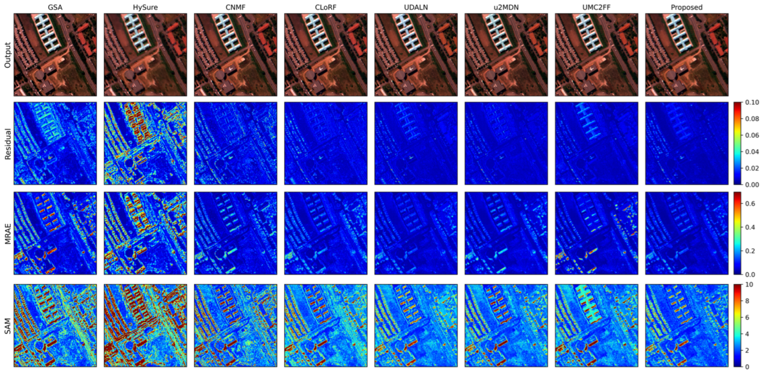
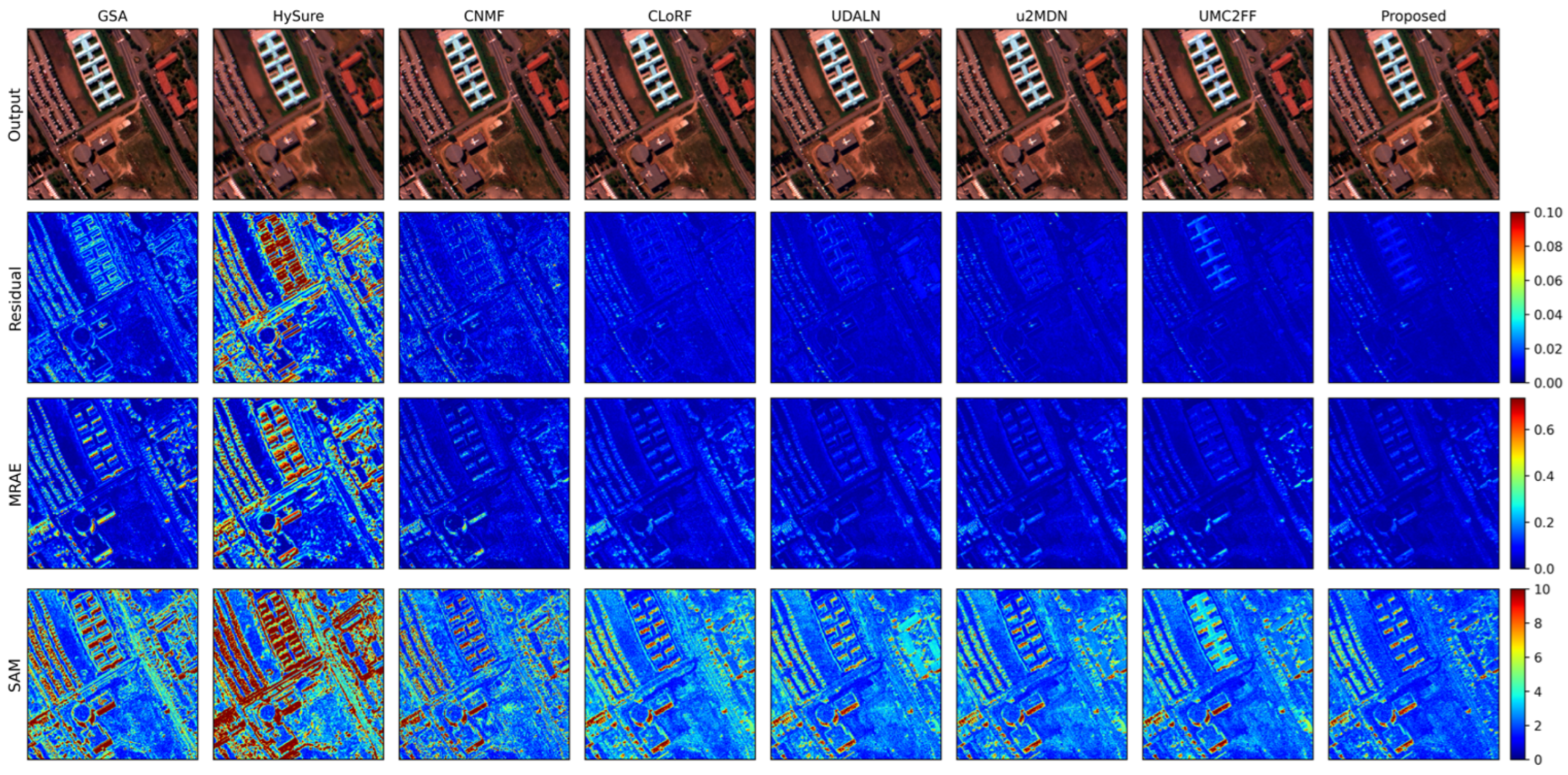
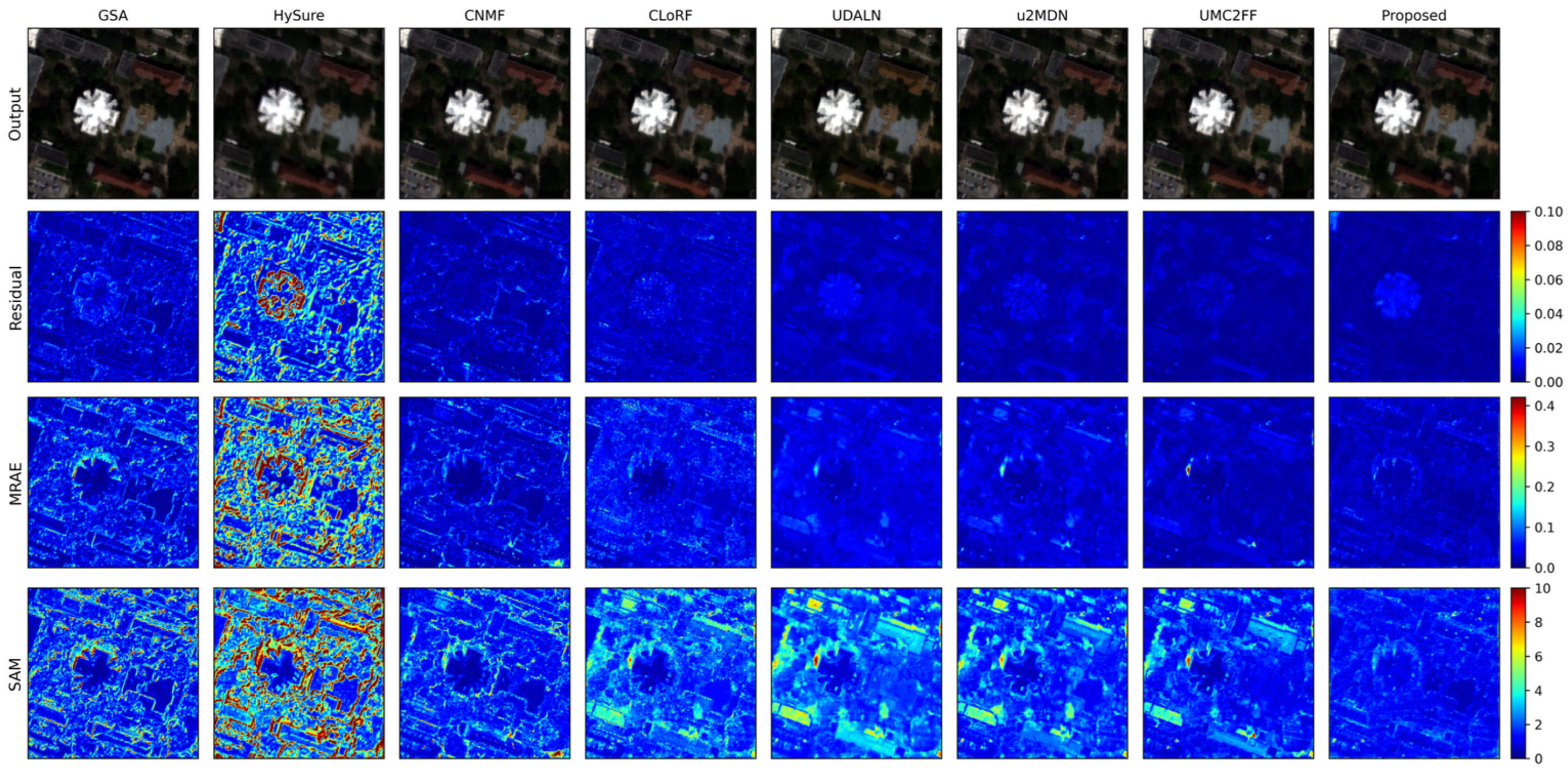
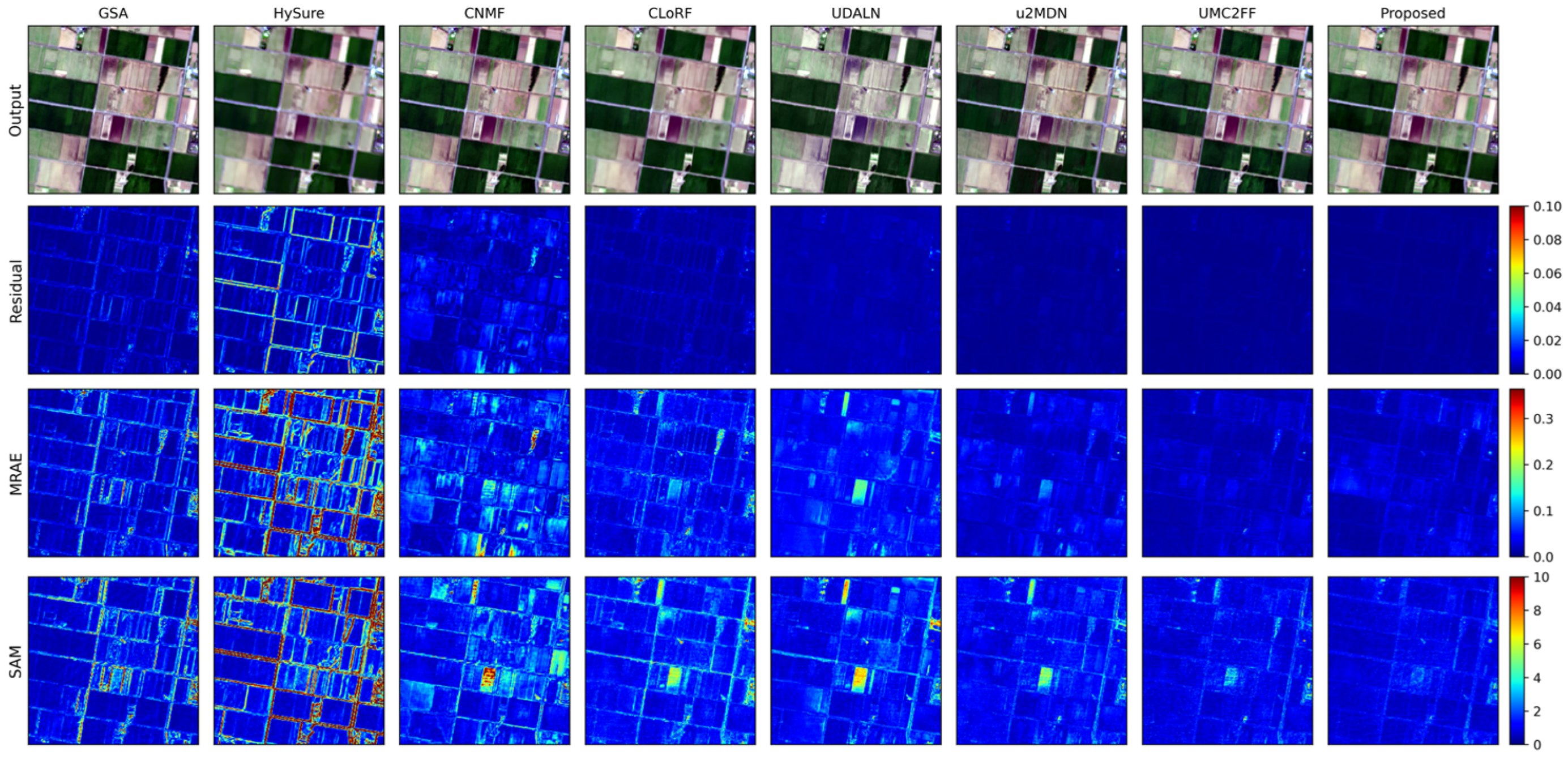
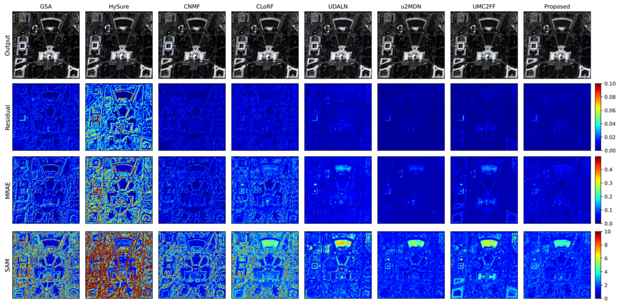
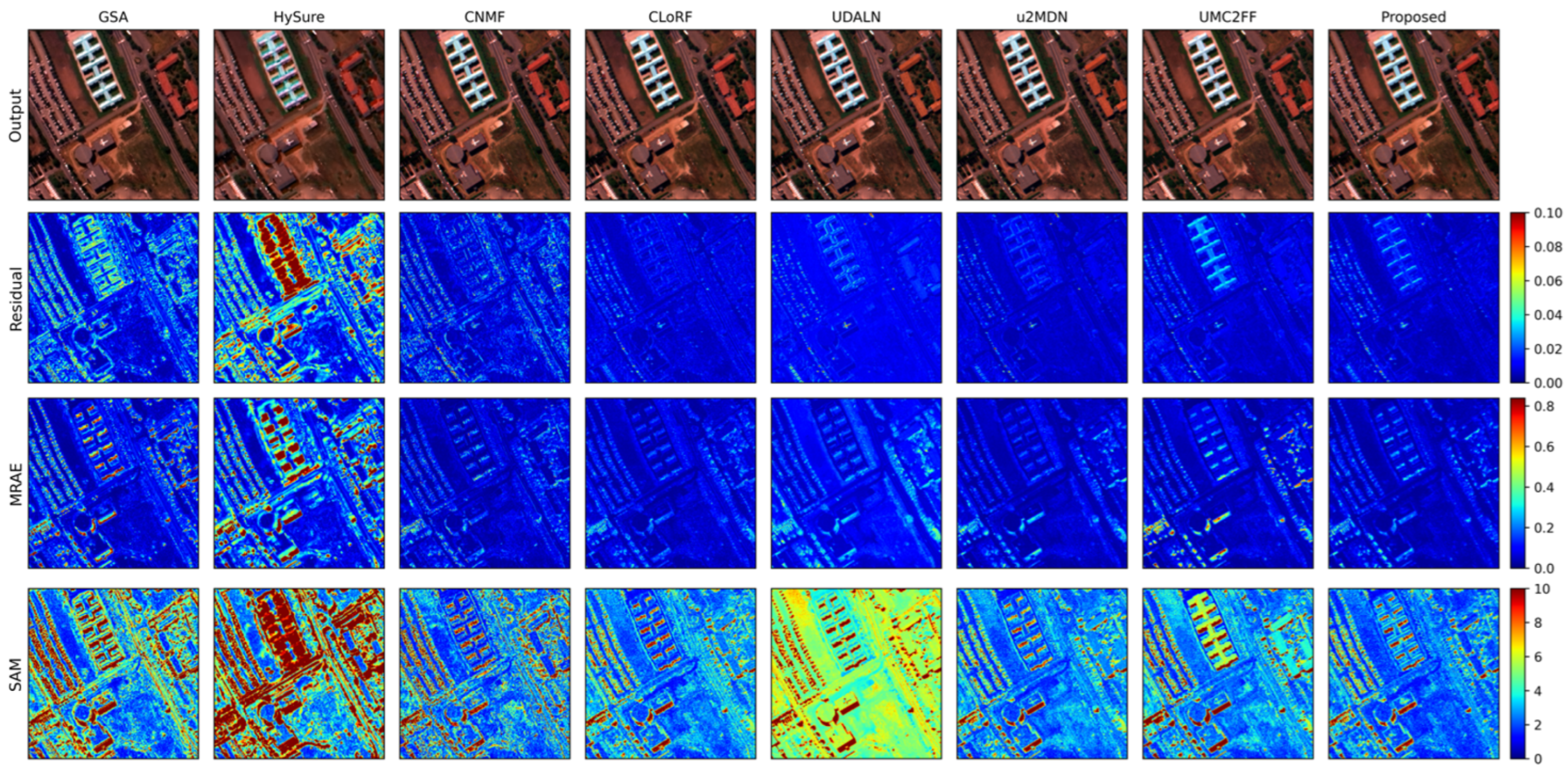
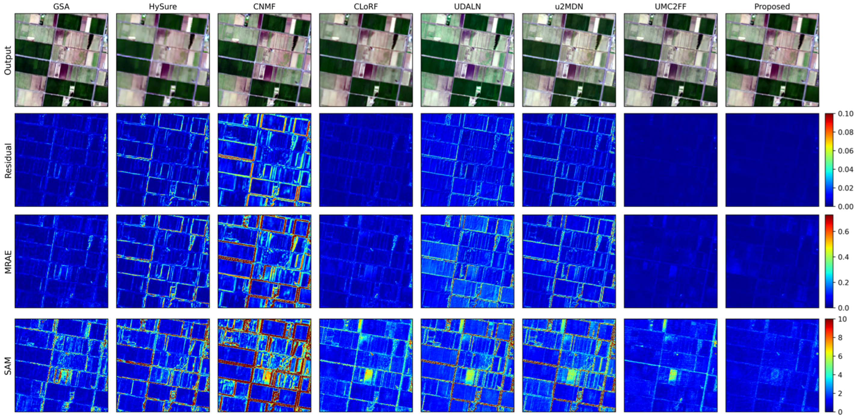
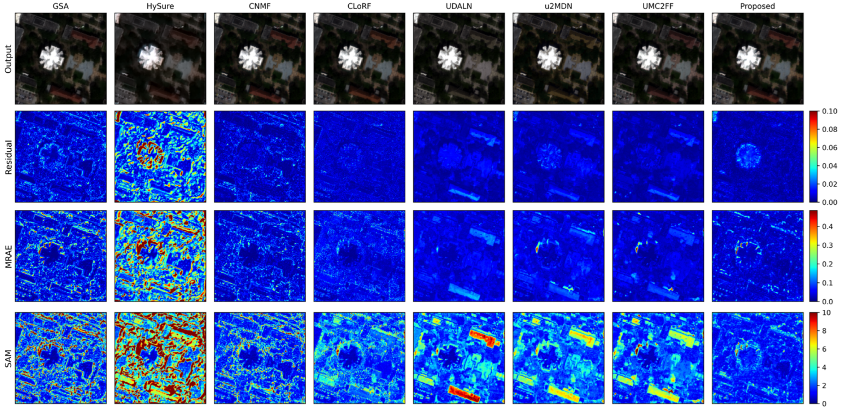
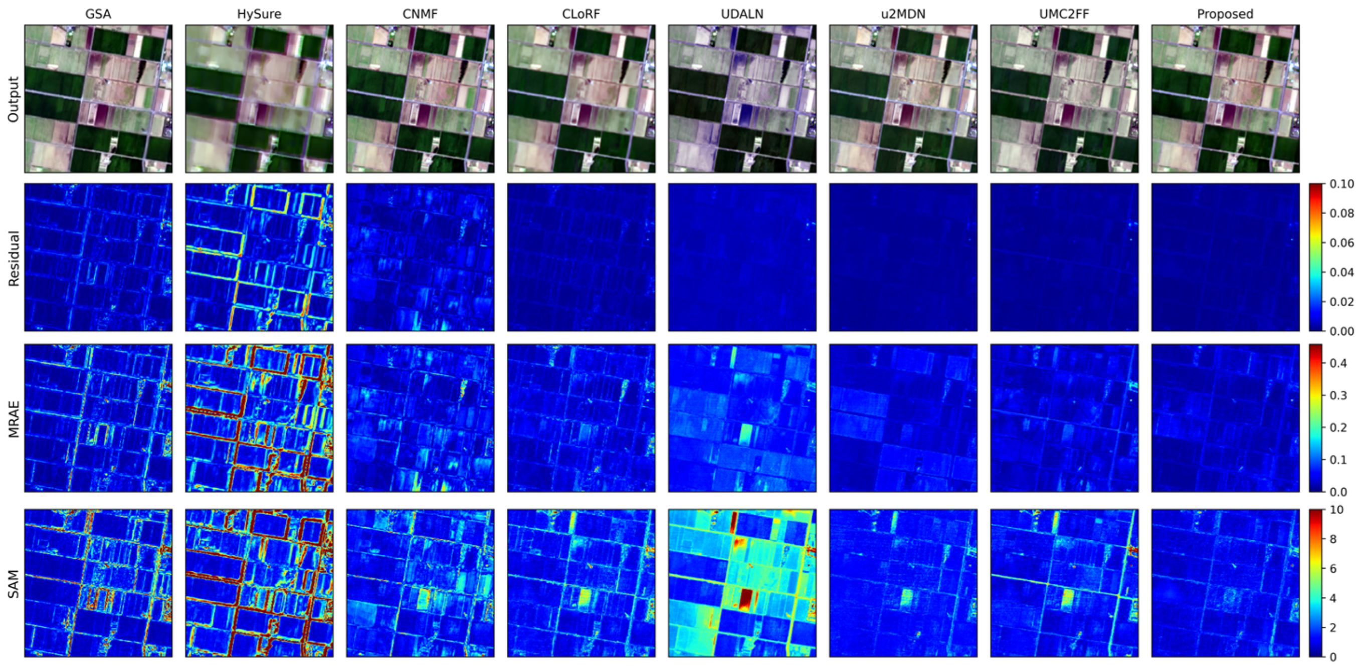
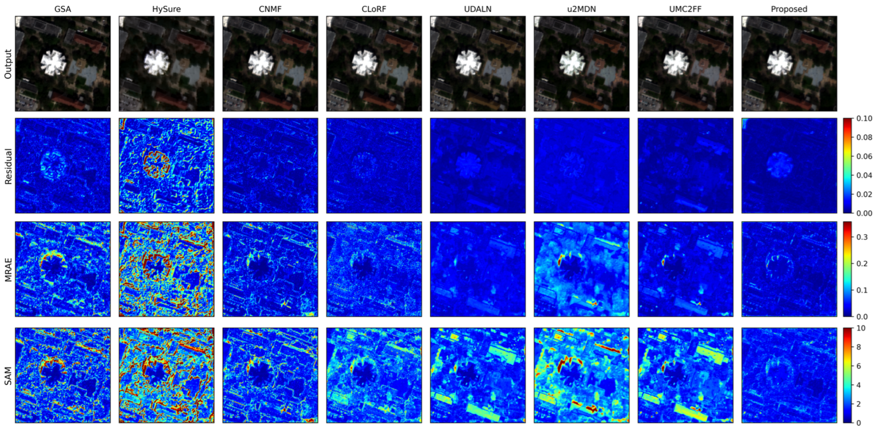
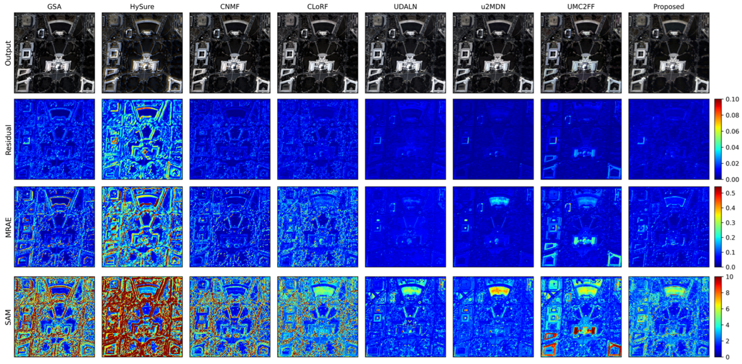
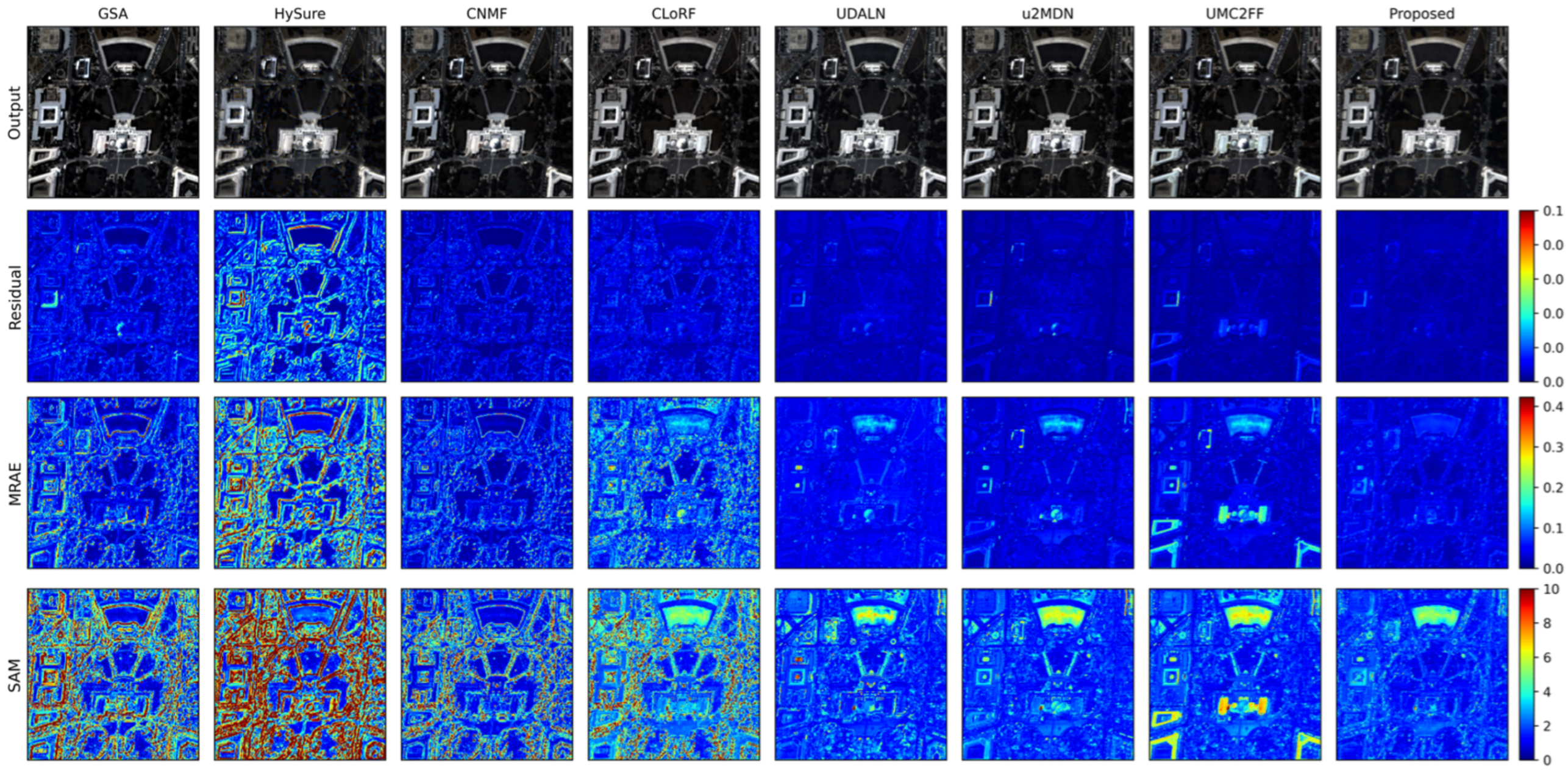
Figure 5, Figure 6, Figure 7 and Figure 8 show the visual comparison results of different fusion methods on PaviaU, Chikusei, Houston18, and WADC at scale factor ×2.4, respectively. For each dataset, the reconstructed images are shown together with residual, MRAE, and SAM maps to visualize pixel-wise reconstruction errors, relative reconstruction errors, and spectral distortions.

Compared with traditional methods, SCDF-Net produces clearer spatial structures and lower error responses. GSA and HySure tend to generate larger residual values around edges and high-contrast regions, indicating insufficient detail preservation or spectral distortion. CNMF preserves some spectral characteristics but may lose fine spatial structures. Deep learning-based methods improve visual quality compared with traditional methods, but some of them still exhibit noticeable errors around building boundaries, roads, vegetation regions, and field edges.

Across the four datasets, SCDF-Net generally produces lower residual and MRAE responses in structural regions and fewer high-error regions in the SAM maps. On urban scenes such as PaviaU, Houston18, and WADC, the proposed method better preserves building boundaries and road structures. On Chikusei, it maintains clearer agricultural field boundaries and reduces spectral distortion in heterogeneous regions. These visual results are consistent with the quantitative metrics and further demonstrate the effectiveness of the scale-conditioned frequency-domain branch and spatial-domain branch.

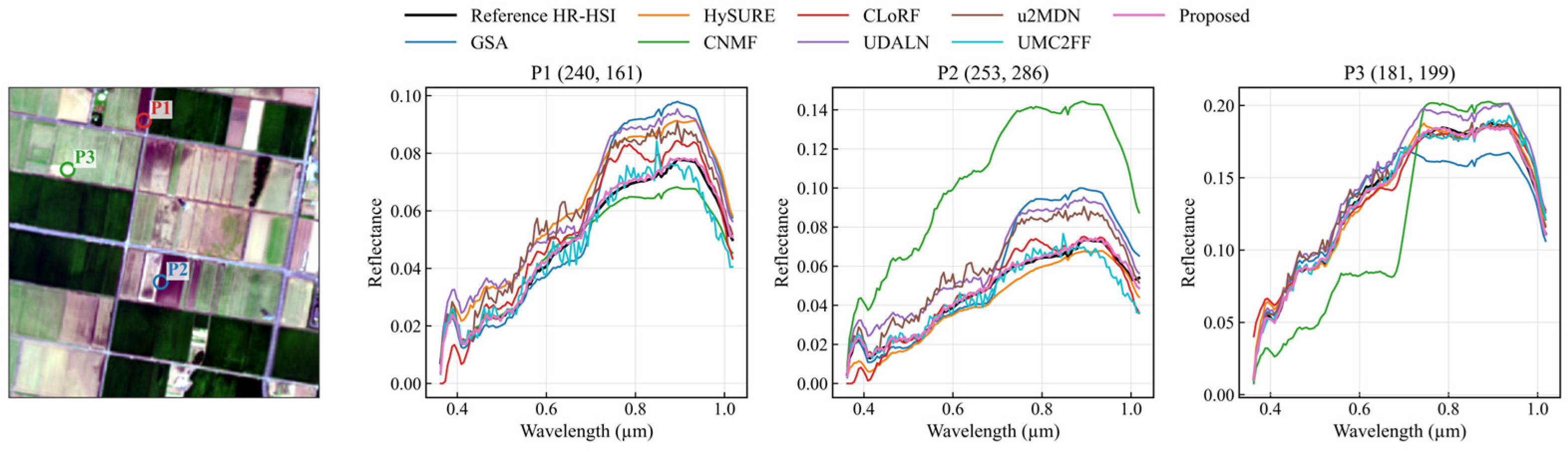
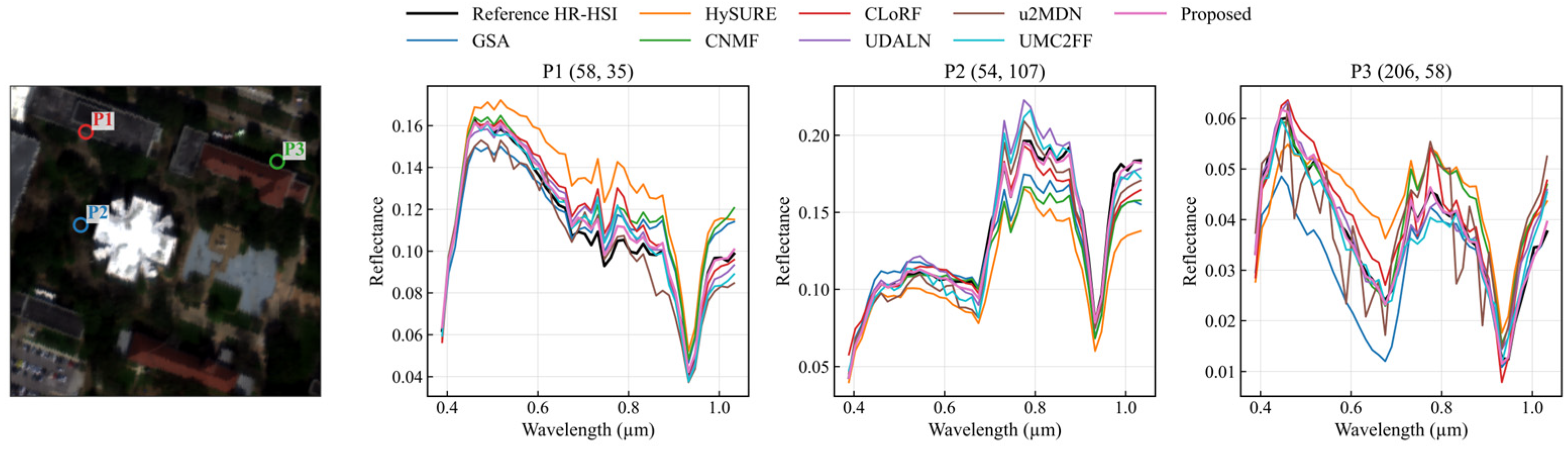
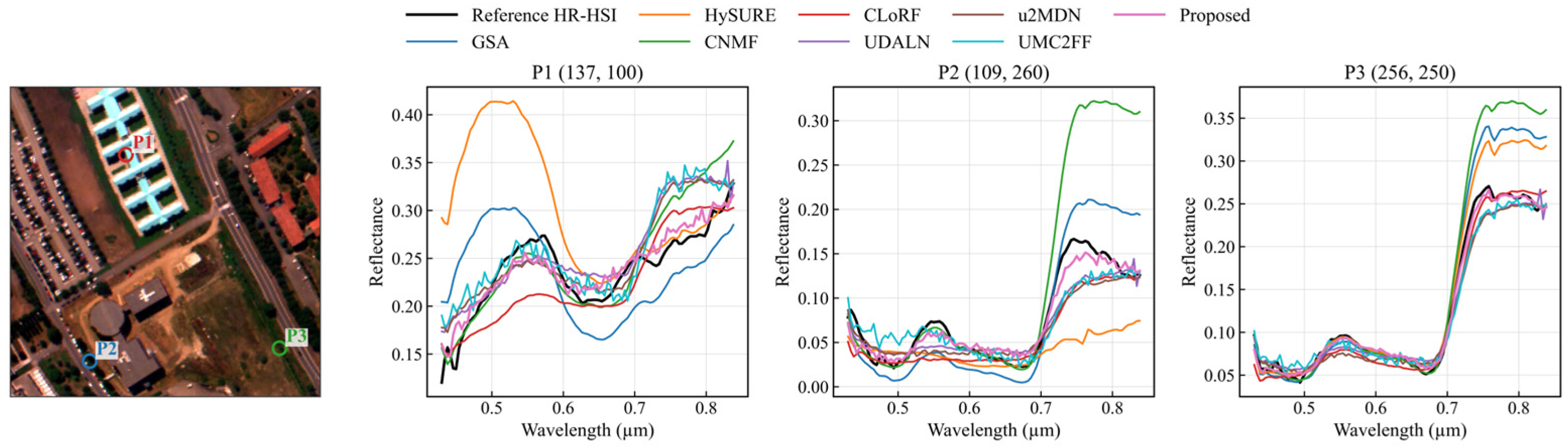
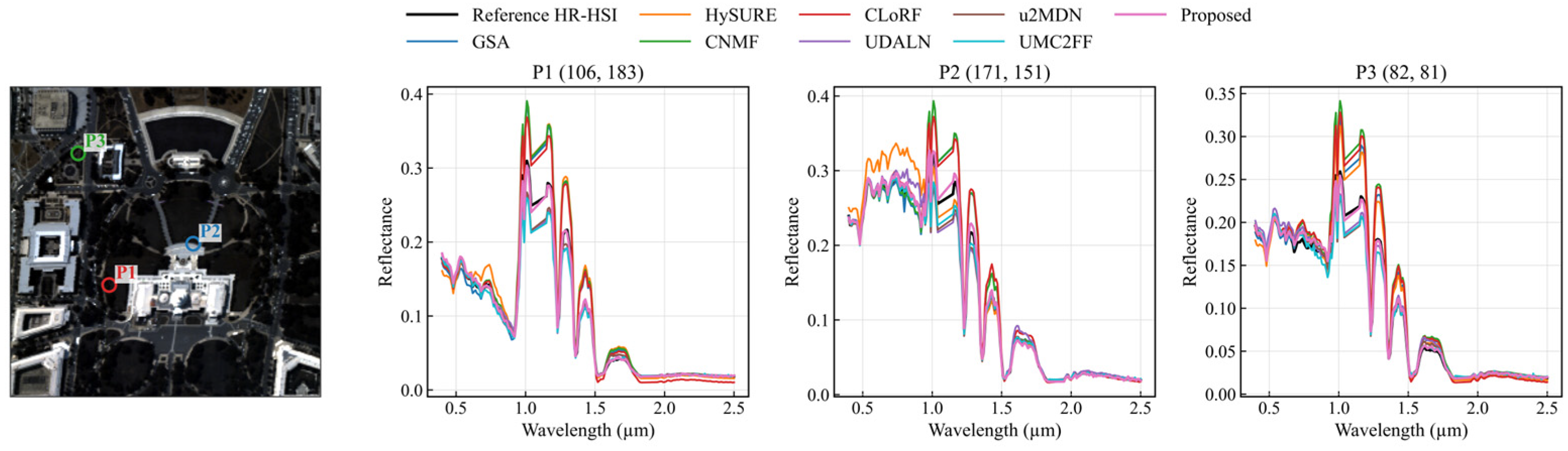
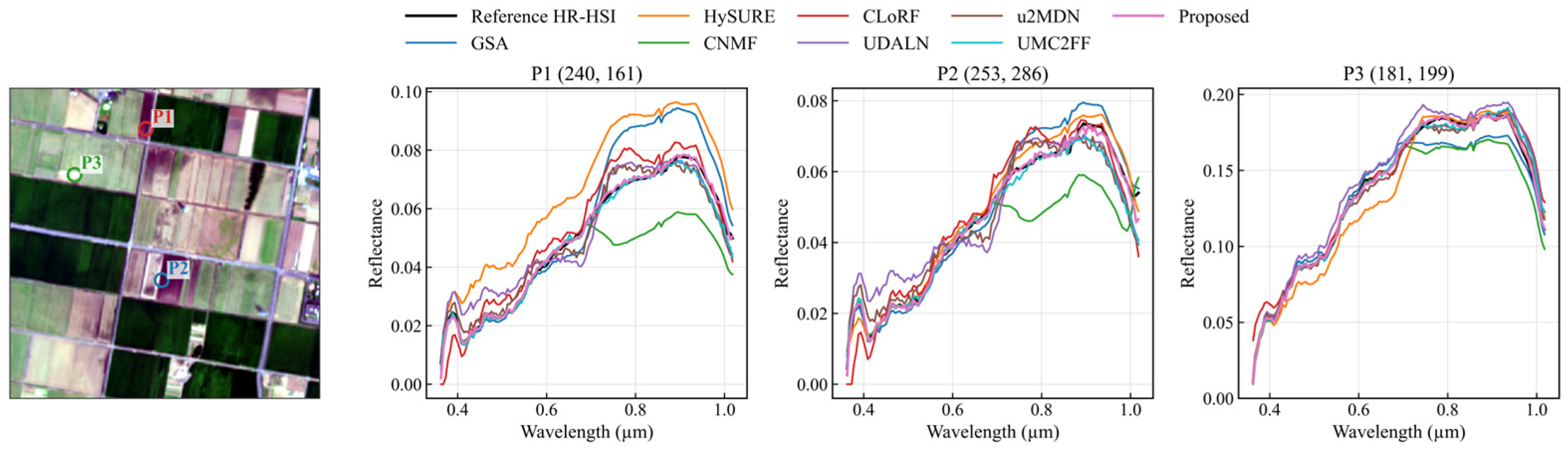
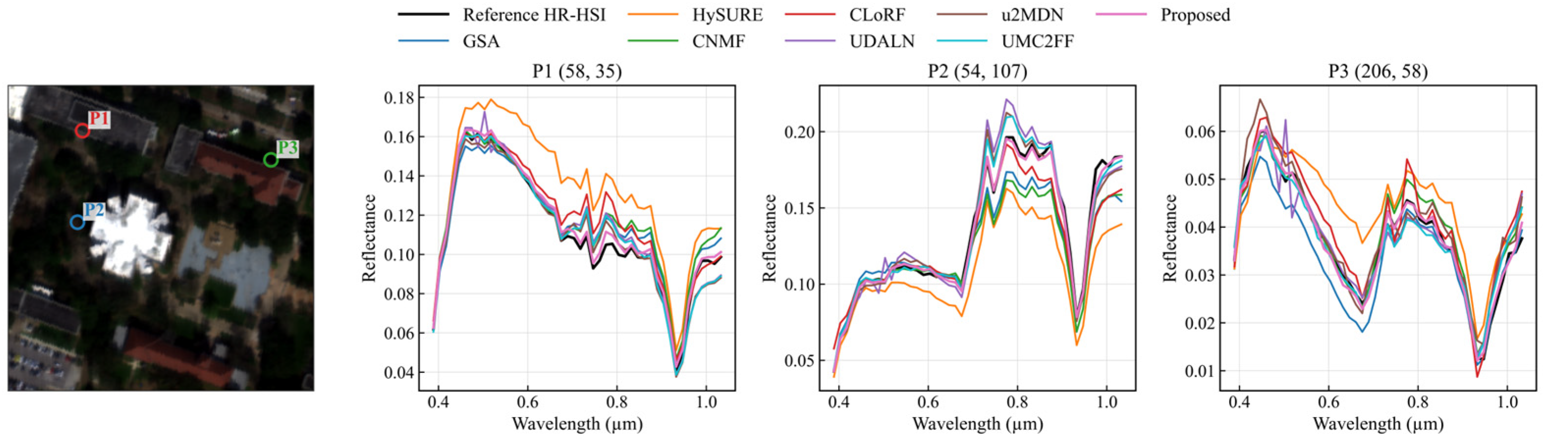
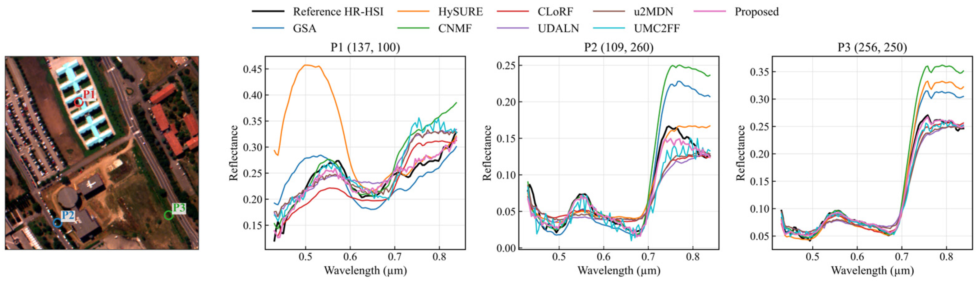
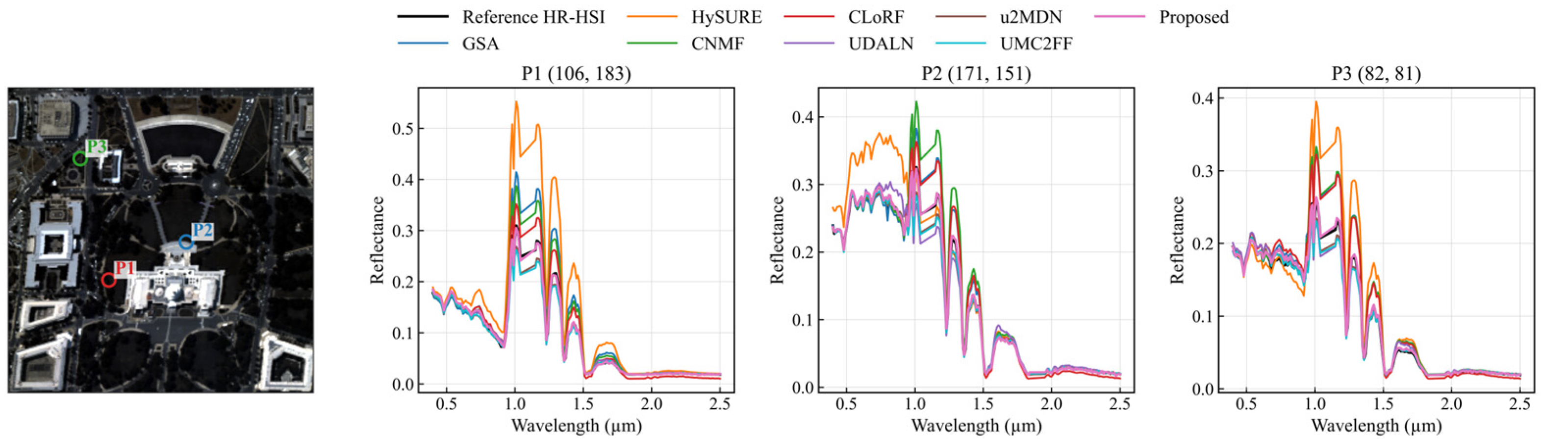
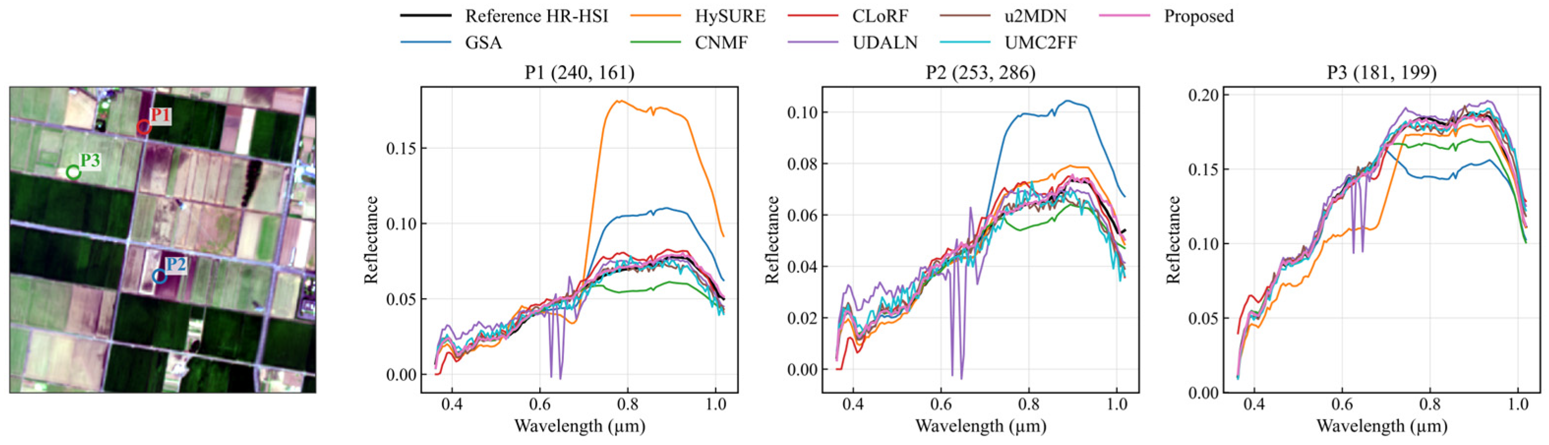
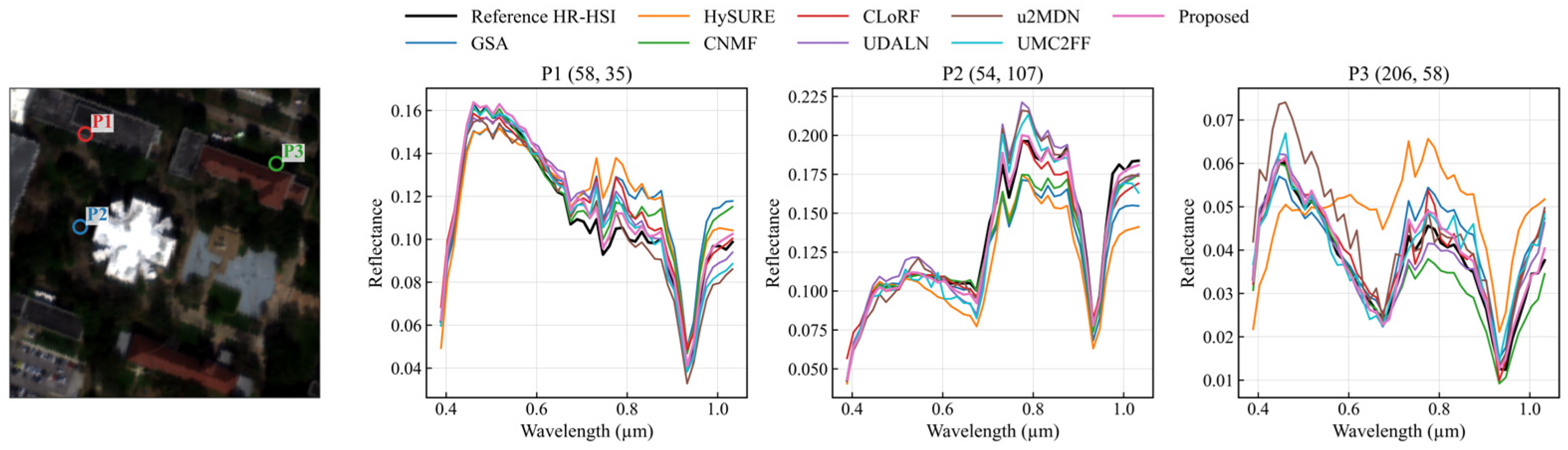
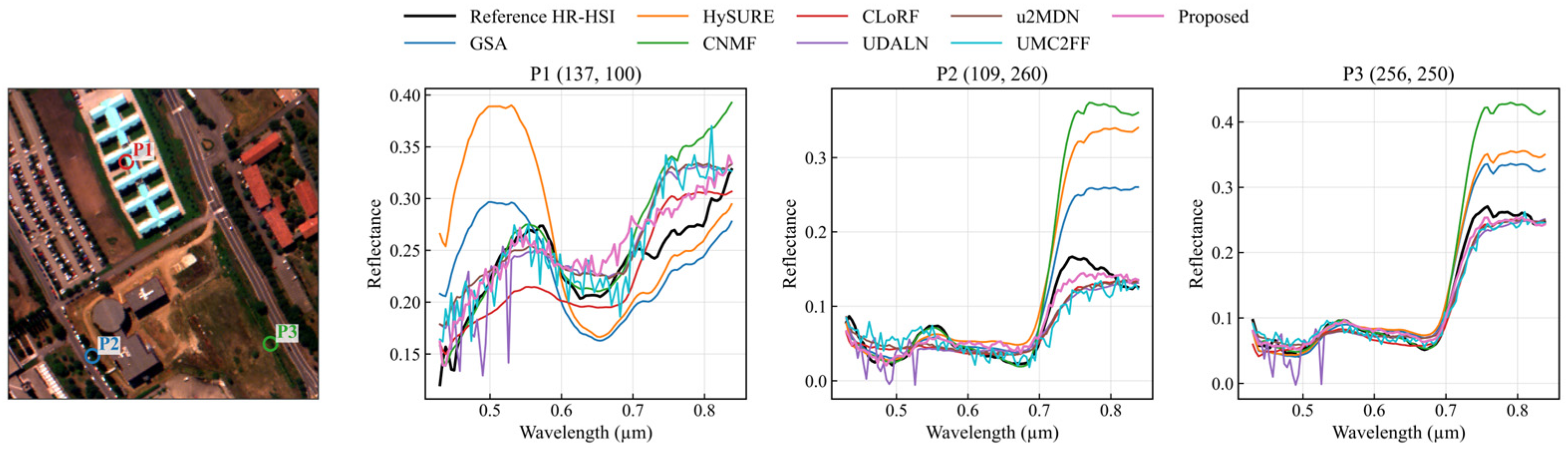
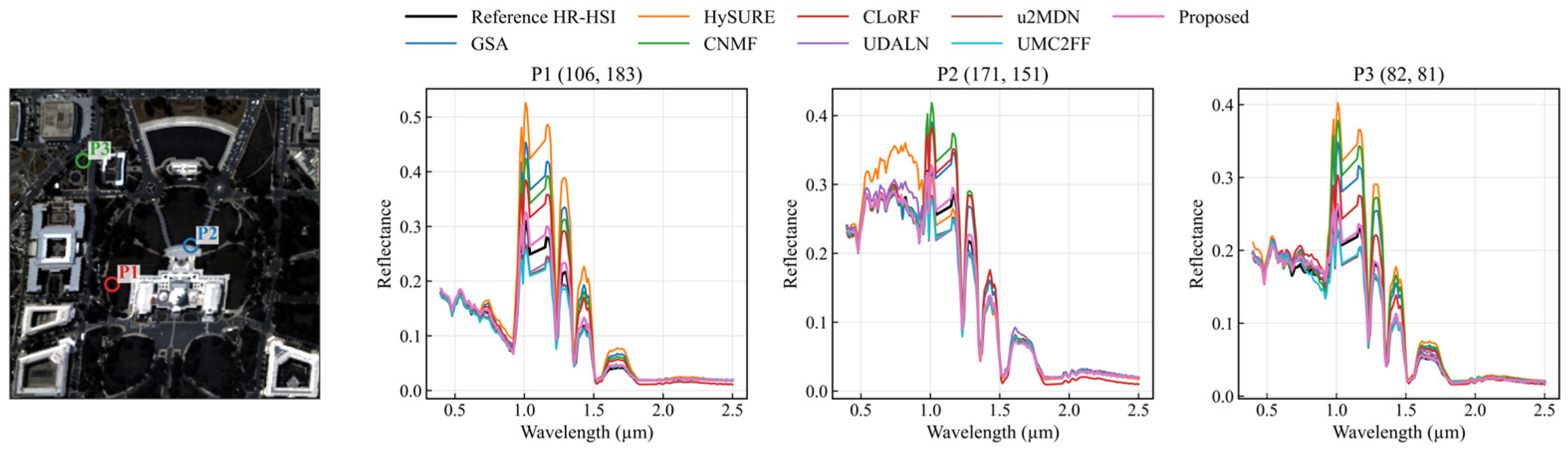
To further evaluate spectral fidelity, we compare the spectral reflectance curves on several representative pixels. Figure 9, Figure 10, Figure 11 and Figure 12 show the results on four datasets at ×2.4 scale. The proposed method generally follows the reference spectral curves more closely than the compared methods at representative pixels, especially in bands where several baselines show visible deviations. This comparison indicates better spectral agreement between the reconstructed and reference spectra. Additional spectral curve comparisons at scale factors ×2.0 and ×4.0 are provided in Appendix A.2 (Figure A9, Figure A10, Figure A11, Figure A12, Figure A13, Figure A14, Figure A15 and Figure A16).

4.7. Ablation Study

To evaluate the contribution of the main components in SCDF-Net, ablation experiments were conducted under scale factors ×2.0, ×2.4, and ×4.0. The ablation study contains two groups of variants. The first group removes network components, including removing both the frequency-domain and spatial-domain branches, removing only the frequency-domain branch, removing only the spatial-domain branch, and removing the scale-embedding module. In the variant without scale embedding, the scale-projection terms are removed from the frequency- and spatial-domain gates, while the remaining branches, losses, and training settings are kept unchanged. The second group removes the two auxiliary loss terms, including W/O L_FREQ and W/O L_SAM. In W/O L_FREQ, the MSI-space frequency consistency loss is removed; in W/O L_SAM, the HSI-space SAM consistency loss is removed. The LV and HV losses are kept in all variants because they provide the main self-supervised observation-domain reconstruction constraints. The results are reported in

Table 12. Ablation results on PaviaU and WADC at scale factor ×2.0.

Variant	PaviaU					WADC
	PSNR	SAM	RMSE	ERGAS	CC	PSNR	SAM	RMSE	ERGAS	CC
W/O FFT and spatial	32.4942	4.2234	0.0237	6.8239	0.9701	42.5548	3.4793	0.0075	5.4002	0.8913
W/O FFT	39.3875	2.9510	0.0107	3.8542	0.9904	44.9117	3.0555	0.0057	4.1508	0.9052
W/O spatial	39.4629	2.9476	0.0106	3.8571	0.9906	44.9712	3.0988	0.0056	4.1573	0.9070
W/O scale-embedding	39.0558	2.9746	0.0111	4.2312	0.9884	44.0968	3.1757	0.0062	4.6303	0.8848
W/O LFREQ	38.9682	3.0139	0.0113	3.9970	0.9898	44.7810	3.0589	0.0058	4.2093	0.9002
W/O LSAM	38.5342	3.1137	0.0118	4.1529	0.9890	44.2764	3.1603	0.0061	4.4754	0.8886
FULL	42.0787	2.4765	0.0079	3.5209	0.9921	48.9587	1.7307	0.0036	2.4797	0.9732

,

Table 13. Ablation results on Houston18 and Chikusei at scale factor ×2.0.

Variant	Houston18					Chikusei
	PSNR	SAM	RMSE	ERGAS	CC	PSNR	SAM	RMSE	ERGAS	CC
W/O FFT and spatial	39.3133	1.9973	0.0108	3.3927	0.9944	42.6445	1.9270	0.0074	7.2028	0.9676
W/O FFT	42.3671	1.6807	0.0076	2.5151	0.9970	45.5622	1.6286	0.0053	5.9358	0.9792
W/O spatial	42.4808	1.6949	0.0075	2.4752	0.9971	46.2633	1.6118	0.0049	4.9084	0.9804
W/O scale-embedding	42.0022	1.7362	0.0079	2.6113	0.9968	44.9825	1.6841	0.0056	6.6327	0.9760
W/O LFREQ	42.6998	1.6298	0.0073	2.4208	0.9973	45.2539	1.6930	0.0055	6.1524	0.9781
W/O LSAM	41.8854	1.7735	0.0080	2.6497	0.9967	44.6196	1.7814	0.0059	6.4250	0.9761
FULL	45.2481	1.3093	0.0055	1.8289	0.9989	50.1400	1.1215	0.0031	4.9887	0.9851

,

Table 14. Ablation results on PaviaU and WADC at scale factor ×2.4.

Variant	PaviaU					WADC
	PSNR	SAM	RMSE	ERGAS	CC	PSNR	SAM	RMSE	ERGAS	CC
W/O FFT and spatial	31.9029	4.0676	0.0254	6.6700	0.9584	41.6876	3.9236	0.0082	5.1540	0.8815
W/O FFT	38.7954	3.0325	0.0115	3.3686	0.9894	44.4227	3.3538	0.0060	2.7520	0.8868
W/O spatial	38.7647	3.0439	0.0115	3.3802	0.9894	44.3844	3.4668	0.0060	3.8060	0.9058
W/O scale-embedding	38.7947	3.0205	0.0115	3.5384	0.9883	44.0648	3.3714	0.0063	4.0722	0.8846
W/O LFREQ	38.2116	3.1951	0.0123	3.5525	0.9883	44.5831	3.3079	0.0059	3.6652	0.9081
W/O LSAM	38.2239	3.1921	0.0123	3.5486	0.9883	43.6720	3.4992	0.0066	4.0683	0.8867
FULL	40.4373	2.7202	0.0095	2.0629	0.9912	47.5650	1.9484	0.0042	2.5664	0.9724

,

Table 15. Ablation results on Houston18 and Chikusei at scale factor ×2.4.

Variant	Houston18					Chikusei
	PSNR	SAM	RMSE	ERGAS	CC	PSNR	SAM	RMSE	ERGAS	CC
W/O FFT and spatial	38.4917	1.8856	0.0119	3.2924	0.9925	41.3166	2.1519	0.0086	6.1997	0.9643
W/O FFT	42.3810	1.6800	0.0076	2.3697	0.9963	45.8048	1.5934	0.0051	4.8752	0.9805
W/O spatial	41.6003	1.7384	0.0083	2.2797	0.9966	46.5533	1.5485	0.0047	2.9746	0.9795
W/O scale-embedding	41.7803	1.6742	0.0081	2.3288	0.9964	44.7756	1.7743	0.0058	3.3158	0.9760
W/O LFREQ	41.7772	1.6805	0.0082	2.2340	0.9968	44.9746	1.7398	0.0056	5.1538	0.9782
W/O LSAM	41.3071	1.8044	0.0086	2.3529	0.9964	45.0309	1.7473	0.0056	5.1904	0.9780
FULL	43.4804	1.3811	0.0067	1.7708	0.9979	49.1500	1.1499	0.0035	4.1706	0.9850

,

Table 16. Ablation results on PaviaU and WADC at scale factor ×4.0.

Variant	PaviaU					WADC
	PSNR	SAM	RMSE	ERGAS	CC	PSNR	SAM	RMSE	ERGAS	CC
W/O FFT and spatial	29.0490	5.1278	0.0353	5.5811	0.9137	39.2786	5.5597	0.0109	4.1333	0.8213
W/O FFT	37.7462	3.2578	0.0130	2.1935	0.9873	42.9348	4.3630	0.0071	3.7320	0.9052
W/O spatial	37.6614	3.3122	0.0131	2.2103	0.9871	43.4478	4.0700	0.0067	2.5896	0.8939
W/O scale-embedding	37.0559	3.4596	0.0140	2.3495	0.9855	43.0936	4.0980	0.0070	4.0722	0.8846
W/O LFREQ	37.5715	3.3203	0.0132	2.2307	0.9869	43.3081	3.8885	0.0068	2.4965	0.8894
W/O LSAM	37.2026	3.4098	0.0138	2.3055	0.9860	43.0288	3.9589	0.0071	2.6749	0.8815
FULL	38.9511	3.0169	0.0113	1.6421	0.9889	45.4189	2.7139	0.0054	1.5319	0.9623

and

Table 17. Ablation results on Houston18 and Chikusei at scale factor ×4.0.

Variant	Houston18					Chikusei
	PSNR	SAM	RMSE	ERGAS	CC	PSNR	SAM	RMSE	ERGAS	CC
W/O FFT and spatial	39.7246	1.8628	0.0103	3.0338	0.9811	42.6352	1.9277	0.0074	5.0579	0.9311
W/O FFT	39.6646	2.0593	0.0104	1.7082	0.9944	45.2977	1.6744	0.0054	2.9788	0.9791
W/O spatial	39.8239	2.0282	0.0102	1.6773	0.9946	45.4155	1.6773	0.0054	2.9746	0.9795
W/O scale-embedding	39.6461	2.0771	0.0104	1.7050	0.9943	44.4603	1.8008	0.0060	5.2186	0.9774
W/O LFREQ	40.0890	1.9685	0.0099	1.6480	0.9951	44.9965	1.7422	0.0056	3.0934	0.9782
W/O LSAM	39.9550	2.0100	0.0101	1.6612	0.9949	44.6228	1.8222	0.0059	3.2010	0.9768
FULL	41.3550	1.6957	0.0086	1.5555	0.9957	47.6500	1.3870	0.0041	2.8290	0.9813

.

Across different scale factors, removing both the frequency-domain and spatial-domain branches leads to the most obvious performance degradation in most cases. The consistent drop shows that direct fusion without explicit frequency- and spatial-domain detail enhancement is insufficient for high-quality HR-HSI reconstruction. When only the frequency-domain branch is removed, the model loses part of its ability to recover high-frequency spatial details. When only the spatial-domain branch is removed, the performance also decreases, showing that local spatial structural guidance is complementary to frequency-domain detail modeling.

The comparison among W/O FFT, W/O spatial, and W/O FFT and spatial further reveals the interaction between the two branches. Removing either branch alone causes a moderate performance drop, whereas removing both branches simultaneously leads to a much larger degradation. This indicates that the frequency-domain and spatial-domain branches are not simply independent add-ons. Instead, they provide complementary information: the frequency-domain branch emphasizes high-frequency spectral–spatial responses, while the spatial-domain branch preserves local structural details in the real domain.

Removing the scale-embedding module also causes consistent performance degradation across different datasets and scale factors. Compared with the full model, the W/O scale-embedding variant reduces the average PSNR by about 3.05 dB over the three scale settings. Although each model targets a single ratio, the low-resolution cycle exposes the scale embedding to a continuous range of cycle ratios ${\mathit{s}}_{\mathrm{LV}}$ during training; the embedding is therefore the signal that informs the frequency- and spatial-domain gates of the current resolution gap.

For example, on the PaviaU dataset at ×2.4 scale, removing the frequency-domain branch alone causes a PSNR drop of 1.6419 dB, and removing the spatial-domain branch alone causes a drop of 1.6726 dB. In contrast, removing both branches simultaneously results in a much larger drop of 8.5344 dB. This larger degradation further supports the complementary interaction between the two branches.

We further evaluate the contribution of the two auxiliary loss terms by removing $L_{\mathrm{FREQ}}$ and $L_{\mathrm{SAM}}$ individually. As shown in Table 12, Table 13, Table 14, Table 15, Table 16 and Table 17, removing either auxiliary loss term leads to performance degradation across most datasets and scale factors. Removing $L_{\mathrm{SAM}}$ mainly weakens spectral-angle consistency and usually increases SAM, while removing $L_{\mathrm{FREQ}}$ reduces the frequency-domain constraint on high-frequency spatial details and leads to lower reconstruction accuracy. These results indicate that $L_{\mathrm{SAM}}$ and $L_{\mathrm{FREQ}}$ provide complementary regularization to the main LV and HV observation-domain losses.

The full SCDF-Net model generally gives the strongest overall results across the ablation tables. The comparison shows that the frequency-domain branch, spatial-domain branch, and scale-embedding module all contribute to the final reconstruction quality. The frequency-domain branch helps recover high-frequency information, the spatial-domain branch provides local structural guidance, and the scale embedding further improves adaptation to different scale factors. Their combination enables SCDF-Net to better preserve spatial details while maintaining spectral fidelity.

5. Discussion

The experimental results on four benchmark datasets demonstrate that SCDF-Net improves both spatial reconstruction quality and spectral fidelity under integer and fractional scale factors. These gains mainly come from the scale-conditioned degradation alignment and the dual-domain detail modeling. The degradation estimation stage provides physically meaningful PSF/SRF priors, which alleviates the ill-posedness of unsupervised fusion. The continuous scale embedding adapts the network to different resolution gaps without resampling inputs to an integer ratio, which is particularly important for fractional ratios. The frequency-domain and spatial-domain branches then recover global high-frequency and local structural details in a complementary manner, while the observation-domain and auxiliary regularizations jointly preserve spectral fidelity. Ablation results further confirm that the frequency-domain branch, the spatial-domain branch, and the scale embedding are mutually reinforcing rather than independent add-ons.

Nevertheless, SCDF-Net still has two main limitations. First, the model contains approximately 3.1 M trainable parameters. Although its inference speed is competitive compared with representative deep learning-based methods, the training and storage costs may limit deployment in resource-constrained scenarios. Second, although the model supports fractional scale factors, its robustness under extremely large resolution gaps and severe spatial degradation has not been systematically validated, especially on real cross-sensor image pairs. Future work will therefore focus on developing more lightweight architectures for efficient training and deployment, and extending the framework to broader scale settings, severe degradation conditions, and real cross-sensor acquisition scenarios.

6. Conclusions

This paper proposes SCDF-Net, an unsupervised scale-conditioned framework for hyperspectral–multispectral image fusion under integer and fractional spatial resolution ratios. The proposed method addresses the fusion of LR-HSIs and HR-MSIs under both integer and non-integer spatial resolution ratios without requiring ground-truth HR-HSIs for training. To improve degradation consistency under fractional scale factors, a two-stage training strategy was developed. In the first stage, the PSF and SRF were estimated from the observed image pair. In the second stage, the learned degradation operators were frozen as physical priors and used to construct scale-conditioned observation-domain constraints for unsupervised fusion training.

SCDF-Net further introduces a continuous scale embedding module and a scale-conditioned frequency–spatial dual-domain fusion network. The scale embedding conditions the fusion process according to the actual resolution gap between the LR-HSI and HR-MSI. The frequency-domain branch enhances high-frequency spatial details, while the spatial-domain branch provides complementary local structural information. Combined with observation-domain consistency, low-resolution self-supervision, HSI-space SAM consistency, and MSI-space frequency consistency, the proposed framework helps preserve spectral fidelity and spatial details during reconstruction under different target scale factors.

Experiments on four benchmark datasets demonstrate that SCDF-Net maintains stable reconstruction performance under both integer and fractional scale factors. Quantitative comparisons show that SCDF-Net achieves the strongest overall performance in most cases and consistently provides low spectral distortion. For example, at ×2.4 scale on the PaviaU dataset, SCDF-Net achieves a PSNR of 40.4373 dB, which is 0.2922 dB higher than that of UMC2FF, and reduces the SAM to 2.7202°, compared with 3.0014° obtained by UMC2FF. On the Chikusei dataset, SCDF-Net improves PSNR by 3.5901 dB over the strongest PSNR baseline and achieves the lowest SAM of 1.1499°. These quantitative gains, together with the visual results, support the effectiveness of the proposed scale-conditioned dual-domain fusion framework. Visual results further confirm its ability to reduce spatial artifacts and spectral distortions, while ablation studies verify the complementary contributions of the frequency-domain and spatial-domain branches.

Future work will focus on validating the framework on real cross-sensor image pairs, improving computational efficiency, and enhancing robustness to severe misregistration, noise, and multi-temporal differences.