Article

Uncertainty-Based Quality-Control Prioritization for High-Resolution Land-Cover Mapping Under Spatially Disjoint Evaluation

1
Department of Geoinformatics, University of Seoul, Seoul 02504, Republic of Korea
2
AI Technology Research Headquarters, GEOSTORY, Seoul 07566, Republic of Korea
*
Author to whom correspondence should be addressed.
Remote Sens. 2026, 18(18), 3197; https://doi.org/10.3390/rs18183197
Submission received: 22 July 2026 / Revised: 11 September 2026 / Accepted: 14 September 2026 / Published: 17 September 2026

Highlights

What are the main findings?
  • A spatially disjoint holdout evaluates selected raster tiles grouped by map sheet; it does not evaluate complete map-sheet coverage.
  • SegFormer achieved an all-valid-pixel mIoU of 0.7066 and a GT-foreground-restricted mIoU of 0.8163.
  • Deterministic Max-Softmax and 20-pass MC-mean Max-Softmax produced nearly identical pixelwise error-ranking AUROC values.
What are the implications of the main findings?
  • Prediction-based tile prioritization did not exceed the random-order mean under the evaluated 20% queue budget (17.61% versus 20.05%).
  • Under the evaluated configuration, deterministic inference uses fewer forward passes than MC Dropout for similar pixelwise error-ranking point estimates.

Abstract

Conventional map-accuracy metrics do not indicate where limited quality-control effort should be allocated. This study evaluates uncertainty-based ranking for post-mapping quality control of selected 25 cm RGB land-cover image tiles under spatially disjoint testing. The dataset contained 15,535 tiles grouped by 359 map sheets in three regions of the Republic of Korea; 12,613 tiles were used to train U-Net, DeepLabV3+, SegFormer, and Mask2Former. SegFormer achieved the highest numerical all-valid-pixel mIoU, 0.7066 (95% confidence interval: 0.686–0.724), and a ground-truth-foreground-restricted mIoU of 0.8163. Deterministic Max-Softmax yielded an error-detection AUROC of 0.8513, compared with 0.8504 for 20-pass MC-mean Max-Softmax. In a retrospective analysis, mean BALD captured 32.9% of errors at a 20% reference-foreground-normalized budget that requires reference labels. In the separate prediction-based evaluation, prioritizing 20% of the queue without reference labels captured 17.61% of the reported errors, below the 20.05% random-order mean. These percentages use different budget definitions and are not a matched operational comparison. Pixelwise ranking therefore does not establish an advantage for the evaluated tile-level prioritization, and full-sheet performance, labor savings, and generalization to unseen regions remain unverified.

1. Introduction

Land-cover maps support urban planning, environmental monitoring, resource management, and public decision-making. Their operational value depends not only on thematic accuracy but also on timely updating as land surfaces change. The increasing availability of very-high-resolution aerial and satellite imagery has therefore accelerated the use of deep semantic segmentation for thematic land-cover map production [1,2]. Recent studies in Remote Sensing have demonstrated land-cover segmentation with very-high-resolution WorldView-3 imagery [2], multimodal and multitemporal Sentinel imagery [3], efficient cloud-based processing [4], multispectral–LiDAR fusion [5], transformer transfer learning [6], foundation-model adaptation [7], ensemble segmentation [8], diffusion-assisted feature fusion [9], and synthetic training data [10]. Together, these developments show that automated land-cover mapping is becoming more accurate and scalable across sensors and applications.
Thematic land-cover map production nevertheless retains a substantial quality-control burden. Overall accuracy, Cohen’s Kappa, and mean intersection over union (mIoU) summarize map performance but do not identify which locations should be examined first. Pixelwise confidence is also not automatically reliable because modern neural networks can be miscalibrated and overconfident [11]. Consequently, a high average score does not by itself provide an inspection order for a newly produced map.
Predictive uncertainty offers a possible ranking signal. Monte Carlo (MC) Dropout approximates Bayesian model averaging through stochastic forward passes [12], and uncertainty measures derived from class probabilities can identify unstable or error-prone predictions [13]. Recent remote-sensing work has also used entropy to guide adaptation toward uncertain image regions [14]. However, uncertainty has commonly been studied as an acquisition signal for additional annotation or retraining, or as a component of interactive correction. Post-inference map review is a distinct task: the model remains fixed, and uncertainty is used only to order an already produced map for inspection.
Spatial evaluation design is equally important. Random tile-level splitting can place visually similar neighboring tiles in both training and evaluation sets, inflating apparent generalization. Spatially separated validation is an established practice rather than a new method [15,16]. Here, a fixed spatial holdout assigns selected tiles sharing a 1:5000 map-sheet identifier to only one partition. The sheet is a grouping unit, not a claim of complete sheet coverage; this is neither repeated spatial cross-validation nor the bootstrap used later to assess test-sheet sampling variability. Neighboring sheets may remain correlated, and all three sampled regions contribute training data; the target is therefore unseen-sheet-group performance within the represented regions.
The study addresses three questions:
  • How do uncertainty rankings perform under a retrospective reference-conditioned budget and a separately defined prediction-based queue budget?
  • How does deterministic single-pass confidence compare numerically with 20-pass MC Dropout for pixelwise error ranking?
  • Are the observed patterns stable across architectures, regions, review-unit sizes, aggregation rules, and removal of test sheets close to training sheets?
The principal contribution is a quality-control-oriented evaluation structure that separates classification performance, calibration, pixelwise error ranking, threshold sensitivity, and retrospective review prioritization. Four representative architectures are compared using the same spatial holdout, with deterministic confidence distinguished from MC-derived quantities. The study does not introduce a new spatial validation method or measure professional map-editing productivity. Because the retrospective review-budget analysis uses reference foreground pixels for tile aggregation and area normalization, it is a diagnostic of the recorded rankings rather than a directly deployable cost estimate. A separate prediction-based evaluation forms the queue without reference labels and uses references only to score the frozen ordering.

2. Related Work

2.1. Semantic Segmentation for Land-Cover Mapping

Encoder–decoder convolutional networks established semantic segmentation as a standard approach for pixelwise mapping. U-Net uses skip connections to restore spatial detail [17], while DeepLabV3+ combines atrous spatial pyramid pooling with a decoder for multiscale context and boundary refinement [18]. Transformer architectures subsequently extended the receptive field and global-context modeling of segmentation systems. SegFormer combines a hierarchical Mix Transformer encoder with a lightweight multilayer-perceptron decoder [19], whereas Mask2Former formulates segmentation as mask classification with masked attention [20] and can use a Swin Transformer backbone [21].
The recent Remote Sensing literature reflects a broad transition from single-sensor convolutional baselines to multimodal, transformer, ensemble, and foundation-model systems [2,3,4,5,6,7,8,9,10]. A systematic review of 106 land-cover segmentation studies likewise identified encoder–decoder and hybrid convolutional designs as dominant, with growing interest in transformer-based models [1]. Korean studies have reported aerial- and satellite-image training-data construction, CNN- and transformer-based classification, ensemble segmentation, and regional generalization experiments [22,23,24,25,26]. These studies primarily evaluate thematic accuracy; the reliability of a map’s confidence ranking and its use for post-mapping inspection remain less frequently quantified.

2.2. Predictive Uncertainty and Calibration

Softmax probability is often treated as confidence, although confidence and empirical correctness can diverge [11]. MC Dropout provides stochastic predictions from one trained network and supports predictive entropy, mutual information (BALD), and inter-pass variability [12,13,27]. Predictive entropy summarizes total uncertainty in the ensemble-mean distribution, whereas BALD isolates disagreement attributable to the model parameters under the dropout approximation. Temperature scaling adjusts probability calibration on a validation set without changing the rank order of logits [11].
Uncertainty quality should be evaluated separately from segmentation accuracy. This study therefore uses: (i) area under the receiver-operating-characteristic curve (AUROC) and area under the precision–recall curve (AUPRC) for detecting misclassified pixels; (ii) expected calibration error (ECE), negative log-likelihood (NLL), and Brier score for probability calibration; and (iii) sparsification error for evaluating how rapidly residual error declines when uncertain pixels are removed.

2.3. Active Learning, Human-in-the-Loop Systems, and Post-Mapping Review

Uncertainty is widely used to select observations for annotation or correction. Deep Bayesian active learning ranks unlabeled samples for acquisition and subsequent retraining [28]. Human-in-the-loop systems similarly direct expert attention toward uncertain predictions; García Rodríguez et al. applied this principle to land-cover segmentation [29], and surveys in medical imaging have documented its value when expert annotation is costly [30,31]. Uncertainty has also been used to identify noisy labels for relabeling before retraining [32,33].
The present problem differs in both intervention and outcome. The model is not retrained, and uncertainty does not select new training labels. Instead, uncertainty orders an already inferred map, and the response variable is the fraction of known errors encountered under a retrospective reference-conditioned budget or a separately defined prediction-based queue budget. Table 1 summarizes this positioning.

3. Materials and Methods

3.1. Dataset, Screening, and Spatial Partition

Parsing the standardized tile file names across all 12,613 tiles indicates that the imagery was acquired over a three-year multi-date campaign: 2019 (4478 tiles, 35.5%), 2020 (994 tiles, 7.9%), and 2021 (7141 tiles, 56.6%). Per-flight sensor-calibration and atmospheric parameters were not provided in the source metadata schema.
The experiments used standard red, green, and blue (RGB) aerial imagery with a ground sampling distance of 25 cm and associated land-cover labels reported as supplied through the Korean AI Hub program [34]. Input tiles were 512 × 512 pixels. The study class system contains ten foreground classes plus an unclassified/background class (Table 2). The source specification distinguishes broadleaved and coniferous forests, whereas the study preprocessing combines them as forest; these are dataset-derived categories, not a universal land-cover standard.
Provider documentation describes TIFF label masks and polygon geometry in JSON annotations, including a non-target category (DN 100) [34]. This establishes the availability of raster and vector representations, but not the exact polygon-to-raster conversion used for the study subset. The study records do not specify minimum polygon area, boundary generalization, overlap priority, or rasterization rules. We therefore evaluate agreement with the supplied reference masks, not conformance to a documented professional cartographic aggregation standard.
The dataset taxonomy separates fine urban and agricultural features while merging forest types in this study. It has broad conceptual affinities with artificial surfaces, agricultural areas, forest/seminatural areas, and water in CORINE Land Cover, but no one-to-one crosswalk is assumed. CORINE uses 44 classes, a 25 ha minimum mapping unit for areal features, and a 100 m minimum width for linear features [35]. These spatial supports differ substantially from individual 25 cm pixels. Transfer to another taxonomy requires explicit class harmonization and renewed assessment of classwise accuracy, calibration, and error capture; it is not demonstrated by the present results.
Tiles were screened using the criteria recorded in the original workflow: image–label alignment, cloud or shadow obstruction, missing reference labels, near-duplicate neighboring scenes, black-border extent, and information density. Training-set class balancing increased the representation of scarce classes and reduced domination by common classes; this denotes statistical sample selection, not a change in raster resolution. Class balancing was applied only to the training partition before model fitting. Numerical screening thresholds, criterion-specific exclusion counts, the ordering of screening decisions, and class-balancing multipliers are not recorded in the available study description. Consequently, the selection procedure cannot be reproduced exactly from those criteria alone.
The retained tiles do not constitute complete operational map sheets. At the reported size and resolution, one tile has a nominal footprint of 128 × 128 m, or 0.016384 km2. Multiplication by the reported tile counts gives nominal footprint sums of 206.651392 km2 for training, 27.672576 km2 for testing, and 20.201472 km2 for validation (254.525440 km2 in total). These are arithmetic sums before accounting for overlaps, invalid margins, or repeated samples; they are not unique mapped areas or retained-area percentages. Exact retention requires the union of retained valid-pixel footprints and the corresponding original sheet-area denominator. Neither can be reconstructed from sheet counts alone.
Screening may preferentially retain easier, well-illuminated, or information-rich scenes. The results are therefore conditional on that selection and cannot quantify performance on rejected tiles or the unprocessed remainder of a sheet. No shadow-stratified evaluation of retained building or tree shadows was available, so removing strongly obstructed tiles does not establish that residual cast shadows had negligible effects.
The provider metadata schema includes acquisition time, coordinate reference system, image coordinates, and resolution [34]. However, a study-level inventory linking these fields to all 359 sheet groups was not available for this evaluation. Collection date ranges for the complete dataset, camera uniformity, atmospheric conditions, and campaign-specific illumination are therefore not established. Equal nominal resolution should not be interpreted as equal acquisition conditions.
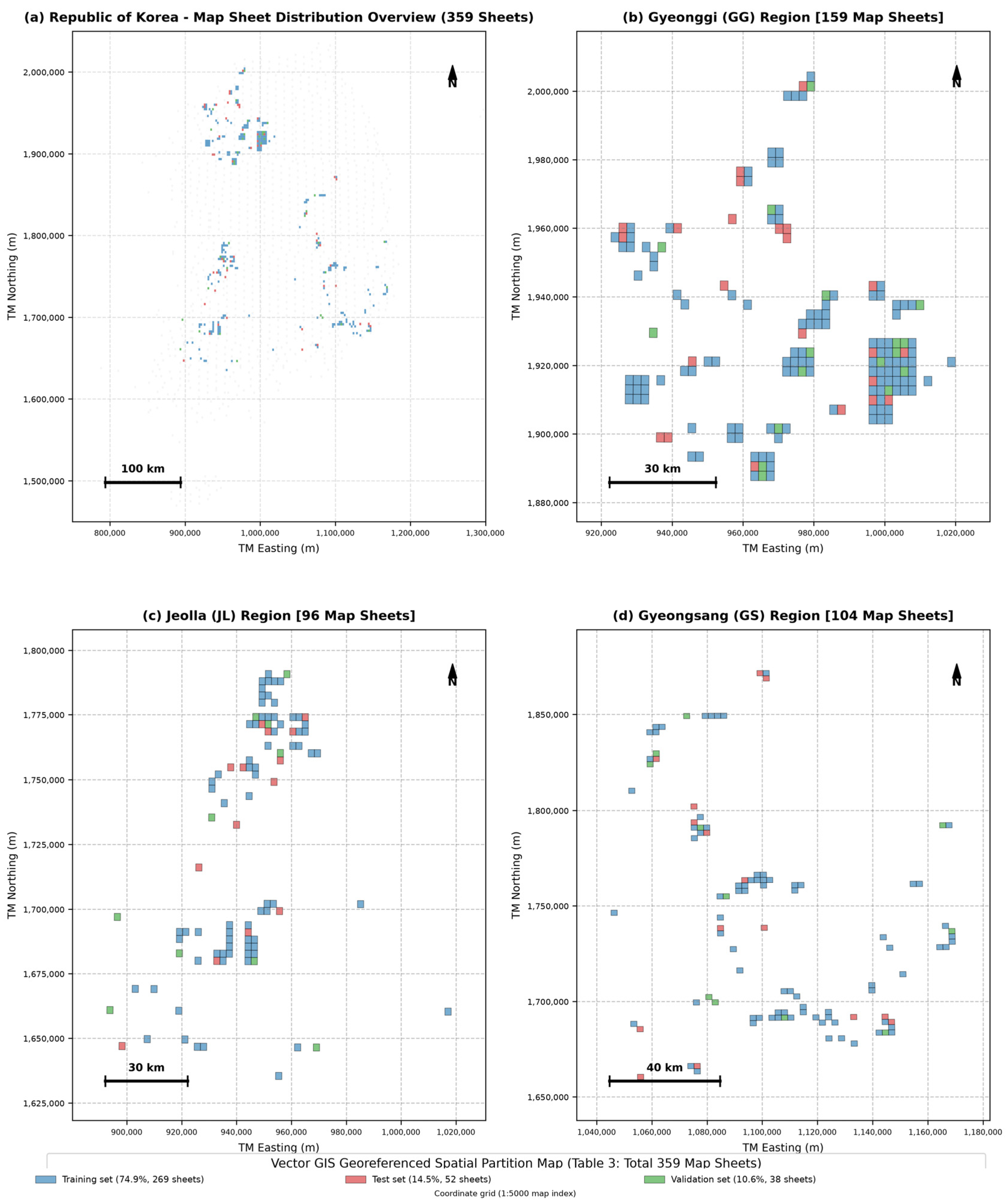
Spatial partitioning used the 1:5000 map sheet as the assignment unit. Every tile belonging to one sheet was assigned exclusively to training, testing, or validation. The 359 sheets comprised 159 in Gyeonggi, 104 in Gyeongsang, and 96 in Jeolla. Sheet counts were 269 training (74.9%), 52 testing (14.5%), and 38 validation (10.6%); the corresponding tile counts were 12,613 (81.2%), 1689 (10.9%), and 1233 (7.9%), respectively (Table 3). Reporting both percentages avoids conflating the sheet-level allocation with the resulting tile-level distribution.
Figure 1 locates the represented regions and preserves the original partition symbols, with the numerical split counts stated explicitly. Symbol overlap in the embedded map cannot be used to estimate partition proportions. The split prevents the same map-sheet identifier from occurring in multiple partitions, but does not by itself eliminate neighboring-sheet dependence, selection bias, or other preprocessing dependencies.

3.2. Segmentation Models and Training

Four architectures were trained and evaluated using the same spatial partitions, loss framework, and augmentation policy (Table 4). U-Net and DeepLabV3+ used ResNet-50 encoders pretrained on ImageNet-1K [17,18]. SegFormer used the ImageNet-1K-pretrained MiT-b2 encoder [19]. Mask2Former used a Swin-L backbone initialized from ImageNet-22K and Cityscapes semantic-segmentation weights; its classification head was reinitialized for the 11 study classes [20,21]. The different parameter counts and pretraining sources were retained as conventional architecture configurations, so comparisons are descriptive benchmarks rather than capacity-matched ablations.
All models produced 11-class predictions, including the background class, which participated in the training objective. Following the original preprocessing workflow, one negative-log-frequency class-weight vector was calculated from the complete labeled-tile inventory and shared by all four architectures; each weight was clipped to the interval [0.1, 10.0]. The weight for class c was
w c = log 10 N c k C N k ,   0.1 w c 10.0
where N c is the number of labeled pixels used to calculate the shared weight for class c , and C = { 0 , , 10 } . A weighted focal term was applied to the final semantic-probability map:
L focal = 1 B H W i = 1 B H W c C w c 1 p i c γ y i c log p i c ,   γ = 2.0
where p i c is the probability of class c at pixel i , and y i c is the corresponding one-hot target. The total objective combined the architecture-native loss and the auxiliary focal term:
L total = L native + α L focal ,   α = 5.0 .
For Mask2Former, L native comprised bipartite-matching classification, binary cross-entropy, and Dice components. For the three pixel-classification models, it was pixelwise cross-entropy. Focal loss was evaluated in an fp32 context under automatic mixed precision to maintain numerical stability.
Under the recorded complete-inventory weighting workflow, class-frequency information was not isolated to the training partition, even though model fitting used training tiles. This preprocessing dependency limits a strict leakage-free interpretation. A training-only recomputation of the weights and refitting would be required to establish its effect; that comparison is not part of the reported results.
The inference workflow contained an optional two-stage background rule. First, a raw class was obtained by maximization over all 11 classes:
c ^ raw x = argmax c C p c x .
The delivered class under the operational rule was then
c ^ final x = c ^ raw x , max c p c x θ bg , 0 , max c p c x < θ bg ,   θ bg = 0.5 .
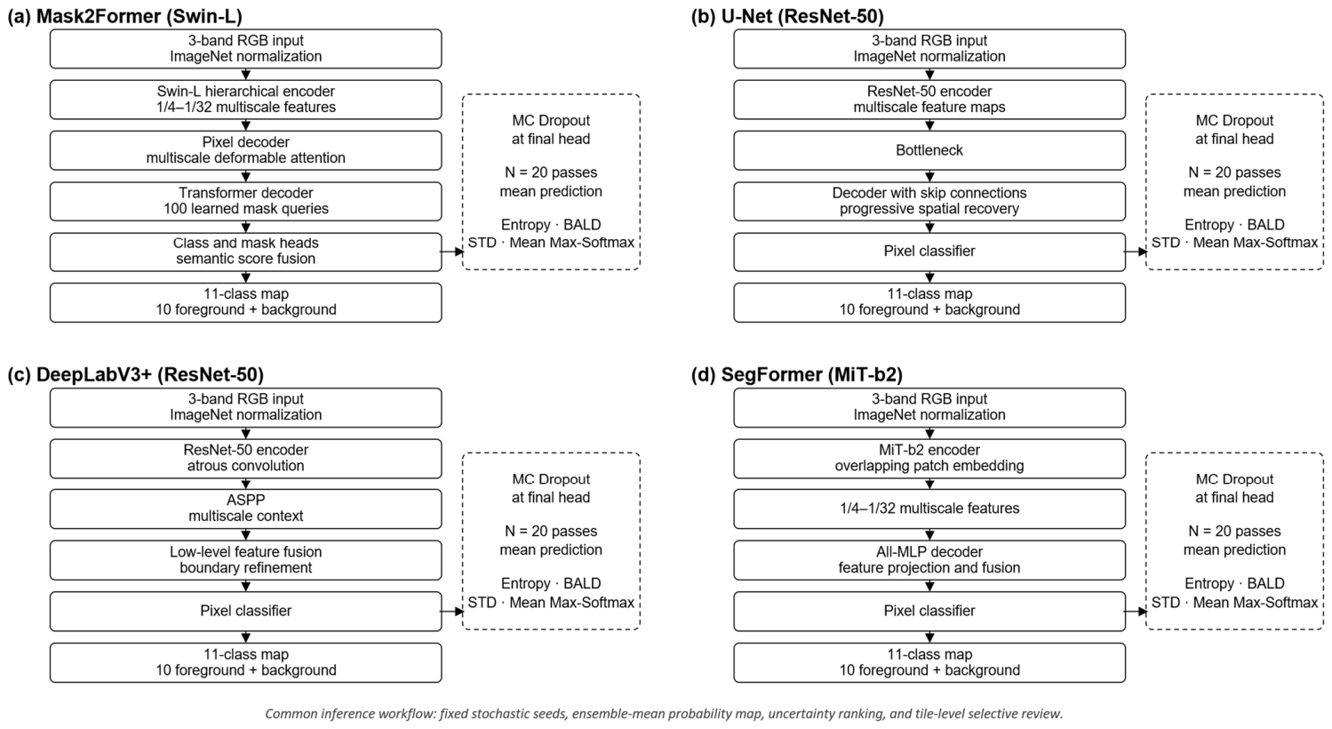
Training used 512 × 512 inputs, AdamW optimization, a polynomial learning-rate schedule, automatic mixed precision, and gradient checkpointing. Augmentation reflected the orientation invariance of nadir imagery: horizontal and vertical flips were each applied with probability 0.5, rotation was randomly selected from 0°, 90°, 180°, and 270°, and brightness was multiplied by a factor sampled from 0.8–1.2. All architectures were trained for 100 epochs. Figure 2 summarizes the architectures and the common stochastic-inference workflow.

3.3. Deterministic and MC-Dropout Uncertainty

MC Dropout was applied to each trained architecture following the approximate Bayesian interpretation of dropout [12]. A dropout layer with probability 0.1 was placed immediately before the final classification head and used consistently during training. At stochastic inference, this layer remained in training mode while the rest of the network remained in evaluation mode. Twenty predetermined random seeds, { 1 , , 20 } , generated N = 20 stochastic class-probability tensors p k . Their mean was
p x = 1 N k = 1 N p k x .
Predictive entropy was calculated from the ensemble mean:
H p x = c = 0 C 1 p c x log p c x + ϵ ,   ϵ = 10 12 .
BALD, expressed as mutual information between predictions and the dropout approximation to model parameters, was
BALD x = H p x 1 N k = 1 N c = 0 C 1 p c k x log p c k x + ϵ .
Inter-pass standard deviation was summarized by the largest classwise standard deviation:
STD x = max c C 1 N k = 1 N p c k x p c x 2 .
Deterministic and MC-mean Max-Softmax uncertainty were kept distinct:
U MSP det x = 1 max c p c det x ,     U MSP MC x = 1 max c p c x .
Here, p det is obtained from one forward pass with dropout disabled. Deterministic entropy was analogously calculated from p det , whereas predictive entropy, BALD, and STD used the 20 stochastic passes. This notation prevents an MC-mean quantity from being described as a single-pass score.

3.4. Evaluation Protocol

3.4.1. Classification Metrics

Two mIoU quantities were retained because they were computed over different evaluation masks. Let Ω all contain every valid pixel, and let Ω GT - FG = { i : y i 0 } contain only pixels whose reference label is foreground. The primary metric was the 11-class mean over Ω all ; the complementary metric was computed after restricting the evaluation mask to Ω GT - FG and averaging the ten foreground classes:
IoU c Ω = T P c Ω T P c Ω + F P c Ω + F N c Ω , mIoU all = 1 11 c = 0 10 IoU c Ω all , mIoU GT - FG = 1 10 c = 1 10 IoU c Ω GT - FG .
Because the second quantity excludes reference-background pixels before constructing its confusion statistics, it is not algebraically derivable from the first and is not labeled as a standard background-excluded mIoU. Overall accuracy, Cohen’s Kappa, macro-F1, and the primary mIoU were evaluated on Ω all .
In mapping terms, IoU measures the overlap between a predicted class and its reference extent, penalizing both missed and falsely assigned area. Restricting the mask to reference foreground removes opportunities to count false foreground assignments on reference background; the restricted score must therefore be interpreted alongside, not instead of, the all-valid-pixel score.
Per-class precision and recall were
Precision = TP TP + FP ,       Recall = TP TP + FN .
The corresponding F1 score was
F 1 = 2 × Precision × Recall Precision + Recall = 2   ×   TP 2   ×   TP + FP + FN .
The relation between classwise IoU and F1 was
IoU = TP TP + FP + FN ,     F 1 = 2 × IoU 1 + IoU .

3.4.2. Error Detection, Sparsification, and Calibration

A pixel was an error when the unthresholded 11-class argmax prediction differed from the reference label. Uncertainty was used as the score for detecting this binary outcome. AUROC was reported together with AUPRC and the error base rate because errors were the minority class. Sparsification removed pixels in decreasing uncertainty order and compared the residual-error curve with an oracle ordering that removes actual errors first. The area between these curves is the area under the sparsification error (AUSE), for which smaller values are better.
For a map reviewer, AUROC describes how well a score places erroneous pixels ahead of correct pixels; 0.5 represents an uninformative ranking. It does not measure whether predicted probabilities are calibrated. AUPRC additionally reflects the prevalence of errors, so comparisons should retain the error base rate. Sparsification asks how much error remains after high-uncertainty pixels are set aside, and AUSE measures the gap from an ideal error-first ordering. These pixel-based diagnostics do not measure the time needed to inspect or edit a cartographic object.
ECE used 15 equal-width confidence bins:
ECE = m = 1 15 B m N px acc B m conf B m .
Temperature scaling fitted one scalar, T , to the validation-set NLL using bounded scalar optimization over [0.5, 5.0] with tolerance 10 4 . The fitted temperature was then fixed for test-set evaluation. NLL and Brier score supplemented ECE.
ECE summarizes discrepancies between confidence and observed correctness within confidence bins. A low ECE alone does not imply high thematic accuracy or strong error ranking; NLL and Brier score provide complementary checks of probability quality.

3.4.3. Threshold-Decoupling Conditions

Three conditions were computed from the same probability tensors. Condition 1 used plain 11-class argmax without a confidence threshold. Condition 2 treated pixels below θ bg as an abstain state and evaluated accuracy only on accepted pixels. Condition 3 applied Equation (5) and reassigned below-threshold pixels to the background. Reporting these conditions separately tests whether the background rule mechanically creates the apparent relation between Max-Softmax uncertainty and error.

3.4.4. Reference-Conditioned and Prediction-Based Review Analyses

The recorded review simulation ranked 512 × 512 tiles by mean uncertainty over pixels labeled as foreground in the reference. The reviewed-area denominator was also the number of reference-foreground pixels, whereas recovered errors were counted over all valid pixels. Thus, reference labels influence both the inspection order and its cost normalization. The resulting 20% budget cannot be constructed by an operator who has no reference map. We retain these values only as retrospective, reference-conditioned diagnostics, not as operational savings or an estimate of how much of a complete map must be reviewed.
The recorded simulation compares the uncertainty curves with a nominal random diagonal and an oracle curve. With variable reference-foreground area per tile and an all-valid-pixel error numerator, a 20% area budget does not establish an empirical 20% random-order expectation. We therefore do not report lift over random as an operational effect size. Sensitivity analyses changed the review grid to 256 × 256 and replaced the tile mean with the median, 90th percentile, 95th percentile, or mean of the upper 10% of uncertainty values.
A separate prediction-based simulation formed the inspection queue from mean BALD over predicted-foreground pixels (pred ≠ 0), without reference labels. Reference labels were used only after the queue was frozen to score captured errors. Its reported 20% budget denotes the top 20% of the queue, rather than 20% of the reference-foreground area. Uniform random-order comparisons used 100 repetitions. The classwise counts are reported in the Discussion and interpreted in Section 5.4. The two review analyses are interpreted separately because the equivalence of their evaluation inventories and error-counting domains is not established. Ranking only predicted foreground can miss foreground-to-background omissions, so a background audit or full-area coverage rule is also needed when adapting this protocol for deployment.

3.5. Reproducibility

The analysis used N = 20 MC samples, dropout probability 0.1, fixed stochastic seeds 1–20, focal-loss parameters γ = 2.0 and α = 5.0 , class-weight clipping to [0.1, 10.0], background threshold 0.5, and 15 ECE bins. Model selection and temperature fitting used the validation partition, and the test partition was used for the reported final metrics and retrospective evaluation. The public QGIS-oriented implementation provides dataset loaders with separate train, validation, and test directories, training-only augmentation, model definitions, uncertainty analysis, and configuration support [36].
Reproduction of the reported experiment additionally requires the exact retained-file and split manifests, screening log, class-weight vector, training configuration, model checkpoints, and prediction/uncertainty exports linked to a fixed code revision. A publicly accessible software repository is not, by itself, a versioned archive of these experimental artifacts. The reported intervals and comparisons remain conditional on the recorded trained models and evaluation outputs.


4. Results

4.1. Classification Performance

The four architectures were evaluated on 1689 test tiles from 52 map sheets. Table 5 reports the two explicitly differentiated mIoU definitions and the all-valid-pixel metrics. SegFormer had the highest numerical mIoU all (0.7066), followed by DeepLabV3+ (0.6750) and U-Net (0.6727). Mask2Former was lower at 0.2858. The complementary mIoU GT - FG was 0.8163 for SegFormer, 0.7806 for DeepLabV3+, 0.7674 for U-Net, and 0.2844 for Mask2Former.
The comparative evaluation includes all four architectures. Relative to DeepLabV3+ and U-Net, SegFormer’s all-valid-pixel mIoU was numerically higher by 0.0316 and 0.0339, respectively. These are differences between the existing point estimates, not paired significance tests. Architecture capacity, initialization, and output formulation differ, so the comparison does not isolate architecture alone.
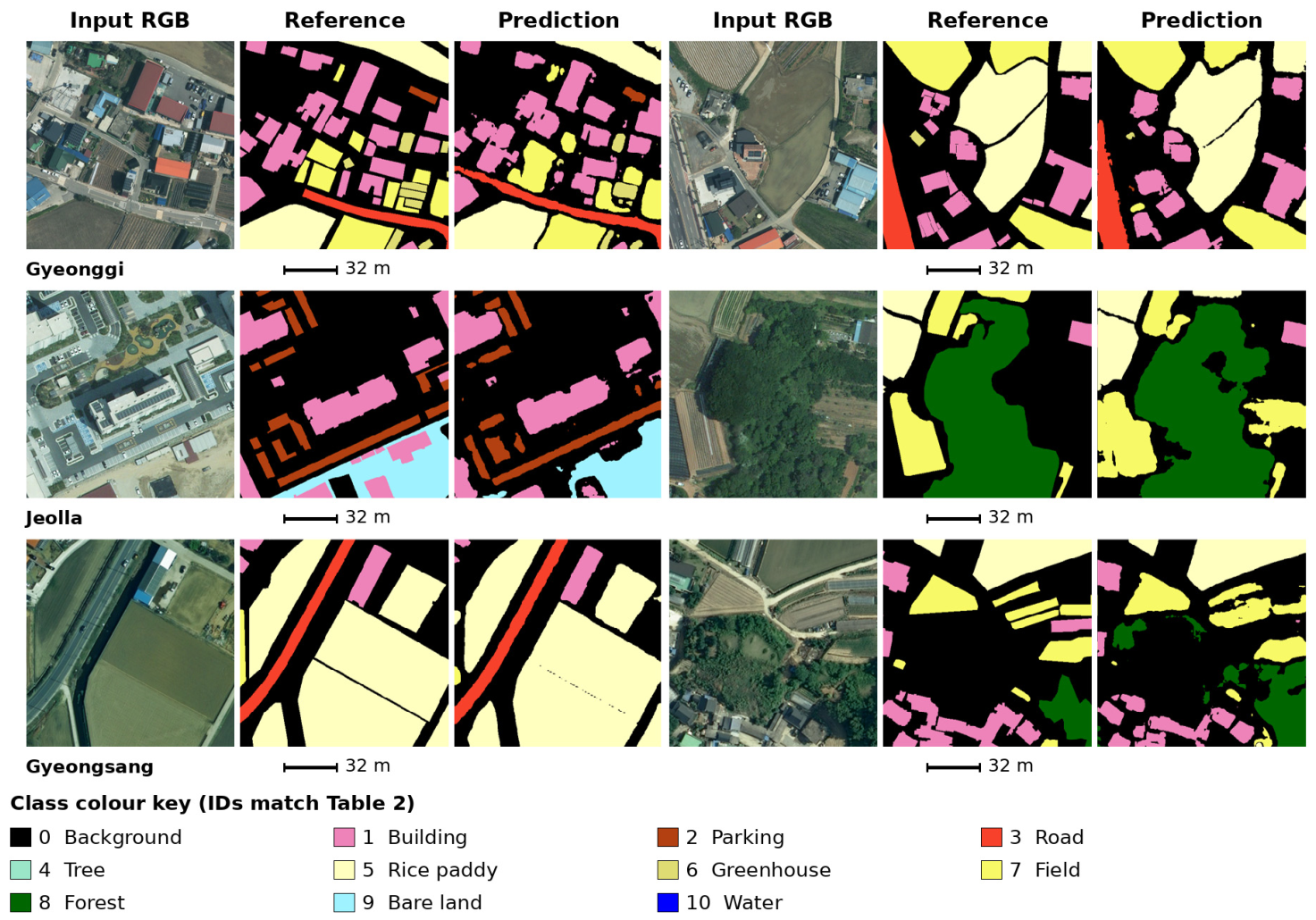
Figure 3 shows SegFormer examples from all three regions; it is an illustration of one model rather than the cross-model benchmark. Major water, building, road, and agricultural boundaries generally follow the reference labels, while some small objects and transition zones remain fragmented or assigned to background. The class-color key and scale annotations support interpretation of these selected examples.
Table 6 separates omission and commission under condition 3 and reports threshold-free error detection under condition 1. The three pixel-classification models showed omission and commission values of approximately 0.09–0.12. Mask2Former showed a different error structure: omission was 0.6925 and commission was 0.0471, indicating that much of its error arose from assigning reference foreground to background. Its AUPRC of 0.5485 must be interpreted relative to its substantially higher error base rate of 0.321.

4.2. Decoupling the Background Threshold from Uncertainty

Table 7 compares the three evaluation conditions. For SegFormer, moving from plain argmax (condition 1) to the background reassignment rule (condition 3) changed mIoU from 0.7066 to 0.7072, an absolute difference of 0.0006. The corresponding differences were 0.0007 for DeepLabV3+ and 0.0029 for U-Net. Mask2Former was more sensitive, decreasing from 0.2858 to 0.2533 because a larger share of pixels fell below the threshold.
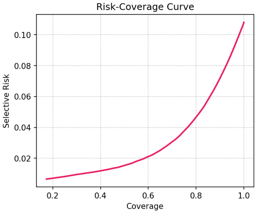
At 98.49% coverage, SegFormer’s selective accuracy was 0.8980, compared with an overall accuracy of 0.8918 at full coverage. Figure 4 places this point on the continuous risk–coverage relation. Selective risk decreases monotonically as the least-confident pixels are deferred, reaching below 0.01 near 20% coverage.
The threshold sensitivity analysis in Table 8 further shows that condition 3 mIoU remains between 0.7066 and 0.7072 for thresholds from 0.3 to 0.5. Above 0.5, coverage falls and mIoU decreases as more foreground predictions are reassigned to background. The threshold of 0.5 was fixed before test evaluation and lies at the upper end of the observed plateau.

4.3. Uncertainty Quality and Calibration

Table 9 compares MC-derived uncertainty measures for detecting misclassified pixels under condition 1. Among the pixel-classification models, MC-mean Max-Softmax produced AUROC values of 0.8270–0.8504, predictive entropy produced 0.8031–0.8262, STD produced 0.7765–0.8137, and BALD produced 0.6969–0.7449. Mask2Former did not follow the same ordering: predictive entropy slightly exceeded MC-mean Max-Softmax, and STD was below random ranking at 0.4615.
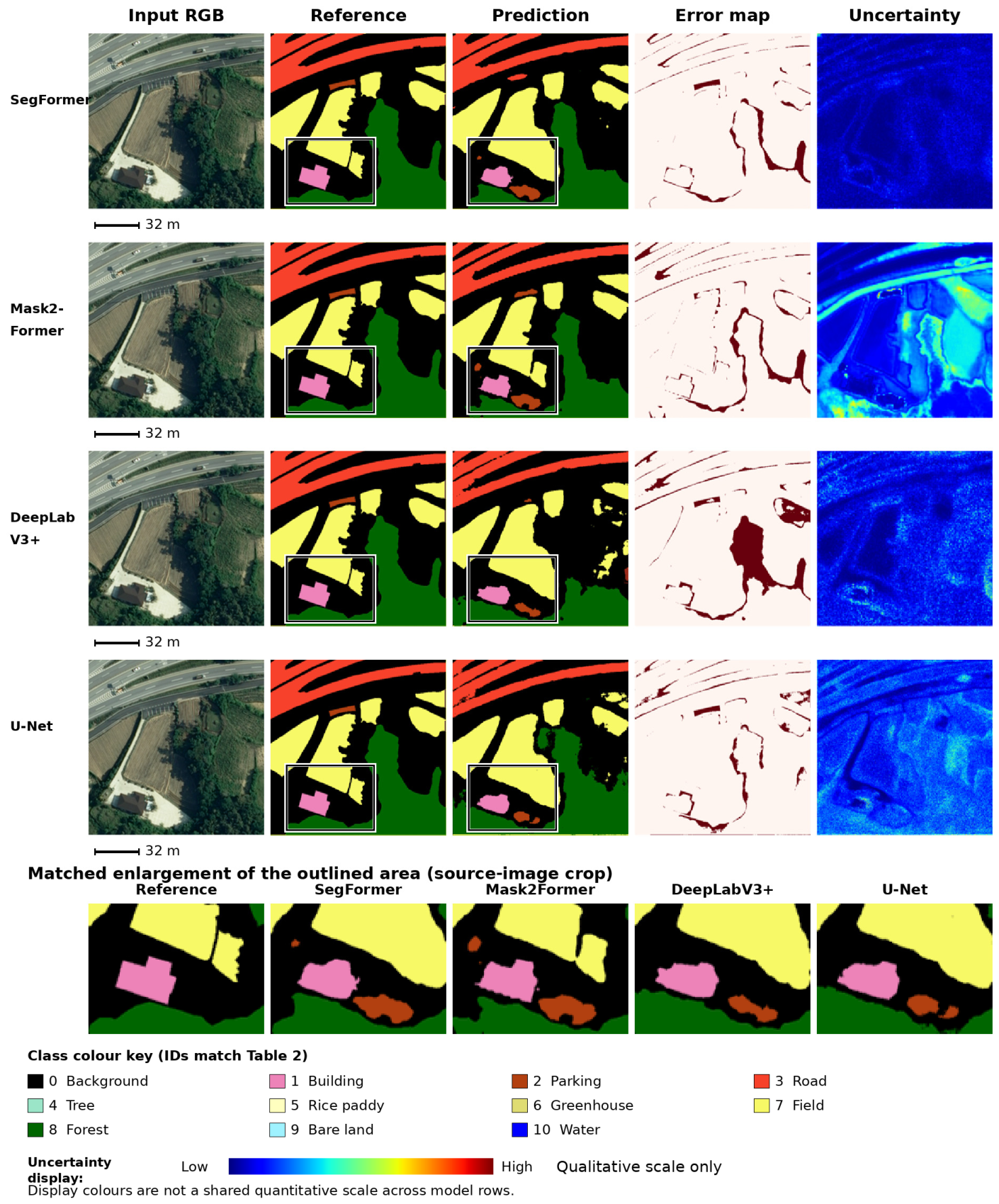
Figure 5 compares all four model outputs, error maps, and uncertainty displays on an identical test tile. Matched enlargements show how the reference building and nearby foreground/background boundaries differ among the displayed predictions. High uncertainty is visually concentrated along some boundaries and transition zones, but the qualitative panels do not quantify boundary-specific error or establish comparable uncertainty magnitudes across models.
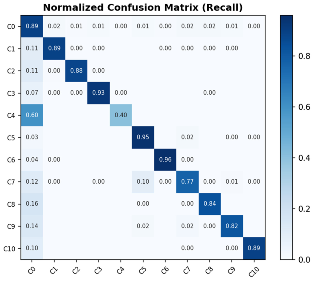
The classwise pattern for SegFormer is shown in Figure 6. Using the class IDs in Table 2, tree (C4) had a recall of 0.40, with 0.60 assigned to the background. Field (C7) had a recall of 0.77, with 0.12 assigned to background and 0.10 to rice paddy. Forest (C8), bare land (C9), and water (C10) had recalls of 0.84, 0.82, and 0.89, respectively. Road, rice paddy, and greenhouse had displayed recalls of 0.93, 0.95, and 0.96, respectively. These values describe classification recall, not the fraction of class-specific errors captured by an uncertainty-based review budget.
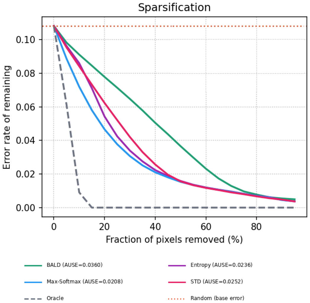
Figure 7 presents SegFormer sparsification curves. MC-mean Max-Softmax had the smallest reported AUSE (0.0208), followed by predictive entropy (0.0236), STD (0.0252), and BALD (0.0360). The curves lie below the random-removal reference over the displayed range, indicating that these pixel rankings contain information about errors. This diagnostic is distinct from the tile-level review budget in Section 3.4.4.
To isolate the numerical effect of stochastic inference, Table 10 compares deterministic single-pass Max-Softmax with MC-mean Max-Softmax. The absolute AUROC difference was 0.0009 for SegFormer, 0.0014 for Mask2Former, 0.0000 for DeepLabV3+, and 0.0004 for U-Net. These differences describe one trained instance of each architecture. They do not establish statistical equivalence, and no measured GPU-time or energy ratio follows from this table.
Table 11 reports the validation-fitted temperatures and the available post-scaling test metrics. The fitted temperatures for the three pixel-classification models were below one, whereas Mask2Former’s temperature was 1.067. Mask2Former retained higher NLL and Brier scores despite a post-scaling ECE of a similar order to the other models, illustrating why calibration should not be summarized by ECE alone. A percentage reduction is not reported because the pre-scaling ECE entries in the original calibration summary were not identical to the corresponding condition-1 entries in Table 5.
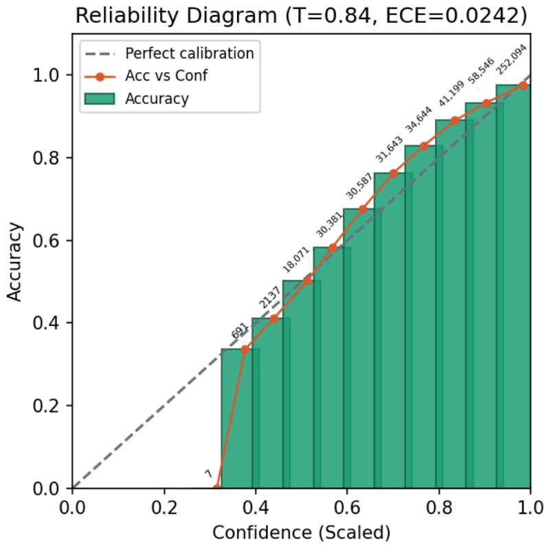
The reliability diagram in Figure 8 is restricted to reference-foreground pixels for readability. Its foreground-only ECE is 0.0242, while the corresponding all-valid-pixel value in Table 11 is 0.0292. The mid-confidence bins lie mainly above the diagonal, consistent with the fitted SegFormer temperature below one.

4.4. Retrospective Reference-Conditioned Review Prioritization

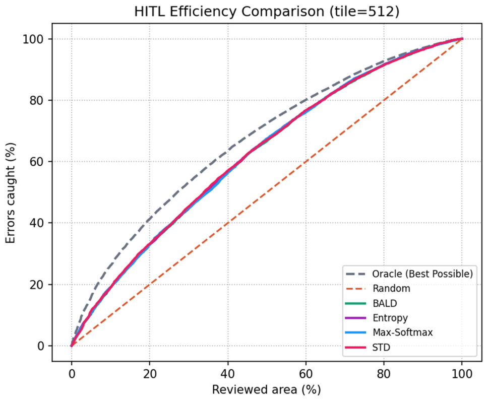
Table 12 reports the recorded mean-BALD analysis at a 20% reference-foreground-normalized budget. Error capture was 32.9% for SegFormer, 28.2% for DeepLabV3+, 26.5% for U-Net, and 21.2% for Mask2Former. These existing values compare reference-conditioned tile rankings across all four architectures. The former lift column is not retained because the nominal 20% diagonal is not a measured random-order baseline under the same variable-area stopping rule.
For SegFormer, changing the review unit and tile statistic produced the results in Table 13. A 256 × 256 grid increased 20% capture from 0.3290 to 0.3586. For the 512 × 512 grid, alternative aggregation statistics produced capture rates from 0.3103 to 0.3290. The required reviewed fractions for recovering 50% and 80% of errors were also reported under the same reference-conditioned normalization.
Figure 9 shows the recorded SegFormer capture curves. At the 20% reference-conditioned budget, the reported capture rates were 32.9% for BALD, 31.4% for STD, 30.9% for predictive entropy, and 30.6% for the curve labeled Max-Softmax. The four-point estimates differ by 2.3 percentage points. The figure alone does not identify whether its Max-Softmax curve used deterministic or MC-mean probabilities; it is therefore not used to quantify a deterministic-versus-MC tile-review advantage. The unambiguous single-pass comparison is the pixelwise AUROC comparison in Table 10.

4.5. Spatial Robustness Within the Sampled Domain

The median distance from a test-sheet centroid to the nearest training-sheet centroid was 10.7 km, and the mean was 18.0 km. Twelve of the 52 test sheets were within 5 km of a training sheet. Re-evaluation after removing these 12 sheets left 40 sheets and 1281 tiles. Table 14 reports the difference between this subset and the full test set. Absolute changes were below 0.005 for mIoU, 0.008 for AUROC, and 0.015 for the 20% capture rate.
Region-wise SegFormer metrics are shown in Table 15. OA ranged from 0.8858 to 0.8979, Kappa from 0.8242 to 0.8512, and error-detection AUROC from 0.8170 to 0.8325. Region-wise mIoU is averaged over the classes present in each regional reference set; because one or two classes are absent in each region, the regional mIoU values do not share an identical averaging set and are not used to rank regional difficulty.
These analyses describe sensitivity across the three represented regions and after excluding the closest test-sheet groups. They do not prove independence of all spatial observations or complete-sheet generalization. Transfer into a region absent from training remains unevaluated.

4.6. Map-Sheet Sampling Variability

Cluster bootstrap intervals were generated by resampling the 52 test map sheets with replacement for 1000 replicates (Table 16). This preserves within-sheet dependence more appropriately than resampling individual tiles. The intervals quantify variability associated with the sampled test sheets for each fixed trained model. They provide marginal intervals for each model, so architecture rankings are described numerically; paired difference intervals can extend this comparison in future work.

5. Discussion

5.1. Scope of the Benchmark and Cross-Model Evidence

This study extends thematic land-cover segmentation evaluation from average classification accuracy to the ordering of potential map errors for inspection. Classification, calibration, pixelwise ranking, and tile-review prioritization answer different questions. The existing four-model tables provide comparative evidence, whereas individual map examples illustrate spatial behavior. Reported advantages are conditional on the selected tiles, model configurations, label definitions, and preprocessing; they are not a benchmark of complete map-sheet production.
The threshold-decoupling experiment helps distinguish raw-probability error ranking from errors induced by a background decision rule. For the three pixel-classification models, plain argmax and background reassignment differed by no more than 0.0029 mIoU; SegFormer changed by 0.0006. This supports the interpretation that the ranking signal is not solely created by the threshold. It does not prove probability calibration, which is assessed separately. Mask2Former was more threshold-sensitive, consistent with its lower accepted coverage, but the comparison does not identify a single causal mechanism.

5.2. Boundaries, Shadows, Acquisition Conditions, and Rare Classes

Because the file-name inventory identifies three acquisition years (2019, 2020, and 2021), differences in seasonal illumination and radiometric conditions across campaigns may contribute to region-to-region variation in predicted uncertainty. We treat this multi-year campaign variance as a qualitative source of domain shift rather than attributing observed error patterns to specific atmospheric causes, because per-flight sensor and atmospheric records were not available.
The classwise errors place the aggregate scores in a mapping context. Figure 6 shows particularly low tree recall and appreciable water-to-background assignment, with additional omission in field, forest, and bare land. RGB ambiguity, small spatial support, heterogeneous boundaries, annotation geometry, and illumination can be compatible explanations, but none was isolated experimentally. Background is a supplied non-target category rather than a complete inventory of physical land covers, so disagreement with it is not automatically proof of a thematic mistake in the real landscape.
At 25 cm sampling, a one- or two-pixel boundary zone is 0.25 or 0.50 m wide. Mixed surface responses, image–label misregistration, roof/tree geometry, and polygon rasterization can produce disagreement near such edges without an interior class error. Conversely, an incorrect homogeneous polygon interior can be confidently wrong. A useful follow-on analysis would report uncertainty ranking and error capture separately for boundary buffers and polygon interiors, with denominators and class frequencies stated. No boundary-buffer analysis was available here, and Figure 5 cannot distinguish these mechanisms quantitatively.
Retained cast shadows and differences in acquisition season, illumination, or atmospheric conditions may alter RGB appearance and confidence. However, shadow masks and campaign-linked metadata were not available for a stratified analysis. Exclusion of heavily obstructed tiles can also suppress the very conditions encountered during routine mapping. These are potential sources of selection and acquisition bias, not demonstrated causes of the reported uncertainty patterns.
The recorded tile statistic averages only reference-foreground pixels, so dominant background does not directly dilute that particular mean. Nevertheless, large foreground classes can dilute localized errors in scarce classes, and the method itself depends on reference labels. Classification recall in Figure 6 is not class-stratified uncertainty recall. Table 17 reports classwise capture for the separate prediction-based evaluation, but it does not provide object-level recall or establish protection of rare or high-consequence classes.
Mask2Former’s result should likewise be read as a configuration-specific interaction between probability formulation and the evaluation pipeline. Query-class probabilities and mask scores are combined differently from a conventional pixelwise softmax. The resulting omission-dominant error, lower coverage, and higher post-calibration NLL and Brier score occur consistently across the reported diagnostics. The finding therefore supports checking the compatibility of pixel-probability thresholds and uncertainty scores with each model’s output formulation, rather than generalizing across all mask-classification architectures.

5.3. Forward-Pass Cost and the Limits of the MC Comparison

For SegFormer, deterministic single-pass Max-Softmax achieved AUROC 0.8513, compared with 0.8504 for the 20-pass MC-mean counterpart. Across the four fixed models, the largest absolute difference was 0.0014. Twenty-pass MC inference requires 20 forward evaluations per input rather than one; single-pass inference therefore uses 95% fewer forward evaluations. This is a pass-count comparison, not a measured 20-fold increase in elapsed GPU time, energy, memory, or monetary cost. Batching, implementation, hardware utilization, and aggregation overhead can change those ratios. The evidence supports a single-pass baseline under the tested head-level dropout probability of 0.1, not universal equivalence of uncertainty methods. Paired sheet-level differences and repeated training would be needed for a formal equivalence or non-inferiority assessment.

5.4. From Retrospective Raster Ranking to Object-Based GIS Review

Computing a review budget from reference-foreground pixels is a retrospective diagnostic rather than a deployable procedure, because reference labels are unavailable when an inspection queue is formed. The separate prediction-based simulation described in Section 3.4.4 instead uses predicted foreground and mean BALD to freeze the queue before reference labels are accessed. In this evaluation, inspecting the top 20% of the queue captured 17.61% of the reported error pixels (1,375,878 of 7,813,786), whereas uniform random ordering captured a mean of 20.05% (100 repetitions; standard deviation, 0.83 percentage points). Table 17 provides the classwise counts. The prediction-based point estimate was below the random-order mean; the evaluated tile-averaging rule therefore did not demonstrate an error-capture advantage over random ordering.
The reference-conditioned and prediction-based results should not be interpreted as the same 20% budget: the former is normalized by reference-foreground area, whereas the latter selects the top 20% of a queue. A matched-cohort comparison with an identical error domain and cost rule would be needed to attribute a numerical difference specifically to reference-label access. The present results therefore do not establish operational lift, labor savings, or measured human-in-the-loop efficiency.
For vector-based GIS review, an uncertainty raster could be summarized over complete predicted or existing editable polygons using area-weighted means, upper quantiles, or boundary/interior summaries. Objects intersecting tile edges should be reunited before prioritization so that a building or field is not treated as several independent edits. Polygon count or observed editing time could then define cost. Raster tiles remain useful processing and navigation units, but their boundaries are not professional cartographic objects. This integration is a proposed workflow, not an implemented or validated component of the present experiment.
An object-only queue would also need an omission safeguard: foreground mapped as background does not necessarily create a predicted object to inspect. Whole-area uncertainty, imagery-assisted candidate detection, or an explicitly sampled background audit could complement polygon prioritization. Translation to another class hierarchy or minimum mapping unit would require separate validation rather than the reuse of the current percentages.

5.5. Remaining Validation and Reproducibility Limits

The fixed sheet-grouped holdout and nearest-sheet exclusion check address direct group overlap and one form of proximity sensitivity; they do not remove all spatial, acquisition, or selection dependencies. The complete-inventory class-weight calculation is an additional limitation. Exact area retention and filtering parameters remain undocumented, and the 359-group acquisition inventory is unavailable. The bootstrap intervals characterize test-sheet sampling for fixed trained models, not training variability or transfer to an unrepresented region. Full-sheet testing, training-only class weighting, matched-cohort review evaluations, measured inspection costs, boundary- and object-stratified evaluation, and a reader study remain necessary before claiming operational performance.

6. Conclusions

An uncertainty-aware evaluation protocol was applied to four land-cover segmentation architectures using a spatially disjoint holdout of selected raster tiles grouped by map-sheet identifier. SegFormer had the highest numerical all-valid-pixel mIoU (0.7066) and GT-foreground-restricted mIoU (0.8163). Deterministic Max-Softmax yielded pixelwise error-ranking AUROC 0.8513, compared with 0.8504 for 20-pass MC-mean Max-Softmax; absolute differences across the four fixed models were at most 0.0014. The main classification result changed little after the removal of the background threshold or exclusion of the closest test-sheet groups.
The recorded reference-conditioned tile-review analysis captured 30.6–32.9% of errors across the four SegFormer uncertainty summaries at a nominal 20% reference-foreground budget. These values are not an operational map-area budget, an independently validated random-order gain, or measured editing savings. In the separate prediction-based evaluation, inspecting the top 20% of the queue without reference labels captured 17.61% of the reported errors, below the random-order mean of 20.05% across 100 repetitions. Thus, tile-averaged predicted-foreground uncertainty alone did not outperform random ordering under the reported queue budget. The reference-conditioned and prediction-based percentages use different budget definitions and should not be interpreted as a matched comparison of operational performance.
A single-pass ranking uses one forward evaluation instead of twenty, but wall-clock and energy benefits were not measured. Confidence provides useful pixelwise error-ranking information in the evaluated selected tiles, but this does not establish an effective tile-level review policy. Complete-sheet mapping, new regions or taxonomies, and polygon-based professional review require further validation with reproducible inputs and deployment-observable costs.

Author Contributions

Conceptualization, I.-H.C. and H.-S.J.; methodology, I.-H.C.; software, I.-H.C.; validation, I.-H.C.; formal analysis, I.-H.C. and H.-S.J.; investigation, I.-H.C.; resources, I.-H.C.; data curation, I.-H.C.; writing—original draft preparation, I.-H.C.; writing—review and editing, H.-S.J.; visualization, I.-H.C.; supervision, H.-S.J.; project administration, H.-S.J.; funding acquisition, H.-S.J. All authors have read and agreed to the published version of the manuscript.

Funding

This work was supported by the Korea Agency for Infrastructure Technology Advancement (KAIA) grant funded by the Ministry of Land, Infrastructure and Transport (MOLIT) under project RS-2022-00141819, “Development of Advanced Absolute, Relative, and Continuous Hybrid Positioning Technologies for the Acquisition of High-Precision Digital Land Information”. This work was also supported by the Institute of Information & Communications Technology Planning & Evaluation (IITP) grant funded by the Korea government (MSIT) (No. RS-2024-00397964, Development of major regional analysis and realization intelligence technology based on micro satellite images).

Data Availability Statement

The source aerial imagery and land-cover-label data are available through AI Hub, subject to its access and use conditions [34]. The QGIS-oriented implementation used for model training, inference, and uncertainty analysis is publicly available at https://github.com/hooni-go/QGIS_GeoActive_ML_Studio (accessed on 22 July 2026) [36].

Conflicts of Interest

Il-Hoon Choi is affiliated with GEOSTORY. The authors declare no other conflicts of interest.

References

  1. Ajibola, S.; Cabral, P. A systematic literature review and bibliometric analysis of semantic segmentation models in land cover mapping. Remote Sens. 2024, 16, 2222. [Google Scholar] [CrossRef] [Scilit]
  2. Sertel, E.; Ekim, B.; Osgouei, P.E.; Kabadayi, M.E. Land use and land cover mapping using deep learning based segmentation approaches and VHR WorldView-3 images. Remote Sens. 2022, 14, 4558. [Google Scholar] [CrossRef] [Scilit]
  3. Wenger, R.; Puissant, A.; Weber, J.; Idoumghar, L.; Forestier, G. Multimodal and multitemporal land use/land cover semantic segmentation on Sentinel-1 and Sentinel-2 imagery: An application on a MultiSenGE dataset. Remote Sens. 2023, 15, 151. [Google Scholar] [CrossRef] [Scilit]
  4. Tzepkenlis, A.; Marthoglou, K.; Grammalidis, N. Efficient deep semantic segmentation for land cover classification using Sentinel imagery. Remote Sens. 2023, 15, 2027. [Google Scholar] [CrossRef] [Scilit]
  5. Chroni, A.; Vasilakos, C.; Christaki, M.; Soulakellis, N. Fusing multispectral and LiDAR data for CNN-based semantic segmentation in semi-arid Mediterranean environments: Land cover classification and analysis. Remote Sens. 2024, 16, 2729. [Google Scholar] [CrossRef] [Scilit]
  6. Chen, M.; Li, L. Hierarchical transfer learning with transformers to improve semantic segmentation in remote sensing land use. Remote Sens. 2025, 17, 290. [Google Scholar] [CrossRef] [Scilit]
  7. Zhang, J.; Li, Y.; Yang, X.; Jiang, R.; Zhang, L. RSAM-Seg: A SAM-based model with prior knowledge integration for remote sensing image semantic segmentation. Remote Sens. 2025, 17, 590. [Google Scholar] [CrossRef] [Scilit]
  8. Dimitrovski, I.; Spasev, V.; Loshkovska, S.; Kitanovski, I. U-Net ensemble for enhanced semantic segmentation in remote sensing imagery. Remote Sens. 2024, 16, 2077. [Google Scholar] [CrossRef] [Scilit]
  9. Shi, Z.; Fan, J.; Du, Y.; Zhou, Y.; Zhang, Y. LULC-SegNet: Enhancing land use and land cover semantic segmentation with denoising diffusion feature fusion. Remote Sens. 2024, 16, 4573. [Google Scholar] [CrossRef] [Scilit]
  10. Clabaut, É.; Foucher, S.; Bouroubi, Y.; Germain, M. Synthetic data for Sentinel-2 semantic segmentation. Remote Sens. 2024, 16, 818. [Google Scholar] [CrossRef] [Scilit]
  11. Guo, C.; Pleiss, G.; Sun, Y.; Weinberger, K.Q. On calibration of modern neural networks. In Proceedings of the 34th International Conference on Machine Learning, Sydney, Australia, 6–11 August 2017; PMLR 70, pp. 1321–1330. [Google Scholar]
  12. Gal, Y.; Ghahramani, Z. Dropout as a Bayesian approximation: Representing model uncertainty in deep learning. In Proceedings of the 33rd International Conference on Machine Learning, New York, NY, USA, 19–24 June 2016; PMLR 48, pp. 1050–1059. [Google Scholar]
  13. Kendall, A.; Gal, Y. What uncertainties do we need in Bayesian deep learning for computer vision? Adv. Neural Inf. Process. Syst. 2017, 30, 5574–5584. [Google Scholar]
  14. Wang, Z.; Zhang, Y.; Zhang, Z.; Jiang, Z.; Yu, Y.; Li, L.; Zhang, L. Exploring uncertainty-based self-prompt for test-time adaptation semantic segmentation in remote sensing images. Remote Sens. 2024, 16, 1239. [Google Scholar] [CrossRef] [Scilit]
  15. Roberts, D.R.; Bahn, V.; Ciuti, S.; Boyce, M.S.; Elith, J.; Guillera-Arroita, G.; Hauenstein, S.; Lahoz-Monfort, J.J.; Schröder, B.; Thuiller, W.; et al. Cross-validation strategies for data with temporal, spatial, hierarchical, or phylogenetic structure. Ecography 2017, 40, 913–929. [Google Scholar] [CrossRef] [Scilit]
  16. Valavi, R.; Elith, J.; Lahoz-Monfort, J.J.; Guillera-Arroita, G. blockCV: An R package for generating spatially or environmentally separated folds for k-fold cross-validation of species distribution models. Methods Ecol. Evol. 2019, 10, 225–232. [Google Scholar] [CrossRef] [Scilit]
  17. Ronneberger, O.; Fischer, P.; Brox, T. U-Net: Convolutional networks for biomedical image segmentation. In Proceedings of the MICCAI 2015, Munich, Germany, 5–9 October 2015; pp. 234–241. [Google Scholar]
  18. Chen, L.-C.; Zhu, Y.; Papandreou, G.; Schroff, F.; Adam, H. Encoder–decoder with atrous separable convolution for semantic image segmentation. In Proceedings of the ECCV 2018, Munich, Germany, 8–14 September 2018; pp. 801–818. [Google Scholar]
  19. Xie, E.; Wang, W.; Yu, Z.; Anandkumar, A.; Alvarez, J.M.; Luo, P. SegFormer: Simple and efficient design for semantic segmentation with transformers. Adv. Neural Inf. Process. Syst. 2021, 34, 12077–12090. [Google Scholar]
  20. Cheng, B.; Misra, I.; Schwing, A.G.; Kirillov, A.; Girdhar, R. Masked-attention mask transformer for universal image segmentation. In Proceedings of the CVPR 2022, New Orleans, LA, USA, 19–24 June 2022; pp. 1290–1299. [Google Scholar]
  21. Liu, Z.; Lin, Y.; Cao, Y.; Hu, H.; Wei, Y.; Zhang, Z.; Lin, S.; Guo, B. Swin Transformer: Hierarchical vision transformer using shifted windows. In Proceedings of the ICCV 2021, Montreal, QC, Canada, 10–17 October 2021; pp. 10012–10022. [Google Scholar]
  22. Lee, S.-H.; Lee, M.-J. Construction and application of artificial-intelligence training data for land-cover mapping using aerial and satellite imagery. Korean J. Remote Sens. 2021, 37, 871–884. (In Korean) [Google Scholar]
  23. Park, H.-K.; Baek, S.-K.; Jung, S.-H. Development of a deep-learning-based ensemble land-cover segmentation algorithm using drone aerial imagery. Korean J. Remote Sens. 2024, 40, 71–80. (In Korean) [Google Scholar] [CrossRef]
  24. Shim, W.-D.; Lee, J.-S. Improving land-cover classification accuracy through a combination of CNN and transformer models. J. Korean Assoc. Geogr. Inf. Stud. 2024, 27, 115–127. (In Korean) [Google Scholar]
  25. Mo, J.-S.; Seong, S.K.; Choi, J.W. Comparative evaluation of deep learning-based building extraction techniques using aerial images. J. Korean Soc. Surv. Geod. Photogramm. Cartogr. 2021, 39, 157–165. (In Korean) [Google Scholar] [CrossRef]
  26. Lee, S.-H.; Kim, J.-S. Land-cover classification using semantic image segmentation with deep learning. Korean J. Remote Sens. 2019, 35, 279–288. (In Korean) [Google Scholar] [CrossRef]
  27. Houlsby, N.; Huszár, F.; Ghahramani, Z.; Lengyel, M. Bayesian active learning for classification and preference learning. arXiv 2011, arXiv:1112.5745. [Google Scholar]
  28. Gal, Y.; Islam, R.; Ghahramani, Z. Deep Bayesian active learning with image data. In Proceedings of the 34th International Conference on Machine Learning, Sydney, Australia, 6–11 August 2017; PMLR 70, pp. 1183–1192. [Google Scholar]
  29. García Rodríguez, C.; Vitrià, J.; Mora, O. Uncertainty-based human-in-the-loop deep learning for land cover segmentation. Remote Sens. 2020, 12, 3836. [Google Scholar] [CrossRef] [Scilit]
  30. Budd, S.; Robinson, E.C.; Kainz, B. A survey on active learning and human-in-the-loop deep learning for medical image analysis. Med. Image Anal. 2021, 71, 102062. [Google Scholar] [CrossRef] [Scilit] [PubMed]
  31. Wang, H.; Jin, Q.; Li, S.; Liu, S.; Wang, M.; Song, Z. A comprehensive survey on deep active learning in medical image analysis. Med. Image Anal. 2024, 95, 103201. [Google Scholar] [CrossRef] [Scilit] [PubMed]
  32. Köhler, J.M.; Autenrieth, M.; Beluch, W.H. Uncertainty based detection and relabeling of noisy image labels. In Proceedings of the CVPR Workshops, Long Beach, CA, USA, 16–20 June 2019; pp. 33–37. [Google Scholar]
  33. Redekop, E.; Chernyavskiy, A. Uncertainty-based method for improving poorly labeled segmentation datasets. In Proceedings of the IEEE International Symposium on Biomedical Imaging, Nice, France, 13–16 April 2021; pp. 1831–1835. [Google Scholar]
  34. AI Hub. Land-Cover-Map Aerial and Satellite Imagery Dataset. Available online: https://aihub.or.kr/aihubdata/data/view.do?dataSetSn=71361 (accessed on 22 July 2026).
  35. Copernicus Land Monitoring Service. CORINE Land Cover. Available online: https://land.copernicus.eu/en/products/corine-land-cover (accessed on 5 September 2026).
  36. Choi, I.-H. QGIS_GeoActive ML Studio. Available online: https://github.com/hooni-go/QGIS_GeoActive_ML_Studio (accessed on 22 July 2026).
Figure 1. Distribution of the selected map-sheet groups. (a) Republic of Korea; (b) Gyeonggi; (c) Jeolla; and (d) Gyeongsang. Panels are redrawn from the official 1:5000 national map-sheet index (TN_MAPINDX_5K) in the UTM-K projection, with metric scale bars, a north arrow, and coordinate grids; training, test, and validation sheets are shown in blue, red, and green, and the counts match Table 3 (269/52/38; 359 total).
Remotesensing 18 03197 g001
Figure 2. Segmentation architectures and common uncertainty workflow: (a) Mask2Former with Swin-L; (b) U-Net with ResNet-50; (c) DeepLabV3+ with ResNet-50; and (d) SegFormer with MiT-b2. Each system produces 11-class probabilities from three-band RGB imagery. Stochastic inference uses N = 20 passes.
Remotesensing 18 03197 g002
Figure 3. Representative SegFormer classifications from Gyeonggi, Jeolla, and Gyeongsang. Each case shows RGB imagery, reference labels, and ensemble-mean prediction. The key lists all ten foreground classes and background, using the class IDs in Table 2. In the reference, black is the supplied unclassified/non-target category (study class 0), not a dark surface or a validity mask; only the designated foreground categories are positively labeled. Its exact mixture of non-target surfaces and annotation omissions cannot be established from this figure. In predictions, background assignment can include missed foreground. The nominal 32 m bars assume that each displayed panel spans the reported 128 m tile width.
Remotesensing 18 03197 g003
Figure 4. Risk–coverage curve for SegFormer on all valid test pixels using unthresholded ensemble probabilities. Coverage is the accepted-pixel fraction, and selective risk is the error rate among accepted pixels.
Remotesensing 18 03197 g004
Figure 5. Qualitative comparison of the four architectures on the same displayed rural transition tile. Columns show RGB imagery, reference labels, predictions, the supplied error display, and the supplied uncertainty display. Outlined regions and matched enlargements are crops of the original panels, not additional predictions. The reference and prediction panels, including the matched enlargements, use the same class-color assignments as Figure 3 (class IDs in Table 2). These categorical colors are separate from the error and uncertainty scales. Dark red denotes highlighted disagreement in the supplied error display. The uncertainty key is qualitative and indicates lower-to-higher display colors within each model row. It does not provide a shared numerical BALD scale; color intensity must not be used for quantitative comparisons between models. Nominal 32 m bars assume a full 128 m tile width; enlargements use a different display scale.
Remotesensing 18 03197 g005
Figure 6. Row-normalized confusion matrix for SegFormer on all valid test pixels. Rows represent reference classes, and each row sums to one. C0–C10 correspond to the class IDs listed in Table 2.
Remotesensing 18 03197 g006
Figure 7. SegFormer sparsification curves on all valid test pixels. Pixels are removed in decreasing uncertainty order. The dashed curve is the oracle ordering, and the horizontal dotted line is the error base rate under random removal.
Remotesensing 18 03197 g007
Figure 8. Foreground-only reliability diagram for SegFormer after temperature scaling ( T = 0.84 ). The dashed diagonal denotes perfect calibration; the tabled ECE values use all valid pixels.
Remotesensing 18 03197 g008
Figure 9. Recorded retrospective reference-conditioned review curves for SegFormer. Error capture is plotted against reviewed reference-foreground area. The line labeled Random is the original nominal diagonal, not a re-estimated random-order baseline. The legacy heading “HITL Efficiency” does not denote measured human inspection time or a reader study. The Max-Softmax inference mode is not resolved by this embedded figure.
Remotesensing 18 03197 g009
Table 1. Positioning of this study relative to related lines of work.
Research LinePrimary ProblemUse of UncertaintyHuman InterventionReported Outcome
High-resolution land-cover segmentation [2,3,4,5,6,7,8,9,10,22,23,24,25,26]Improve thematic classificationUsually not centralNone during inferenceOA, mIoU, classwise accuracy
Spatial generalization assessment [25]Evaluate performance outside training locationsNot usedNoneRegion-wise classification performance
Interactive land-cover correction [29]Correct uncertain segmentationSeparate uncertainty estimatorExpert corrects selected areasAccuracy versus intervention
Label-noise detection [32,33]Improve training labelsSelect suspicious samplesRelabel selected samplesPerformance after retraining
Active learning [28,30,31]Reduce annotation required for model learningAcquisition functionAnnotate selected samplesAccuracy versus annotation budget
This studyOrder an already produced map for retrospective reviewPixel error ranking and tile prioritizationSimulated review order; no retrainingError capture under separately defined reference-conditioned and prediction-based budgets
Table 2. Land-cover classes and label digital numbers used in the study.
IDClassLabel DNRole
0Unclassified/background100Included as the background class
1Building10Foreground
2Parking20Foreground; scarce
3Road30Foreground
4Tree40Foreground
5Rice paddy50Foreground
6Greenhouse55Foreground; scarce
7Field60Foreground
8Forest70Foreground
9Bare land80Foreground
10Water95Foreground; scarce
Table 3. Map-sheet and tile counts by region and partition.
RegionTotal SheetsTraining Sheets/TilesTest Sheets/TilesValidation Sheets/Tiles
Gyeonggi (GG)159119/714123/82217/636
Gyeongsang (GS)10478/323115/41211/391
Jeolla (JL)9672/224114/45510/206
Total359269/12,61352/168938/1233
Percentage of sheets100%74.9%14.5%10.6%
Percentage of tiles100%81.2%10.9%7.9%
Table 4. Segmentation architectures evaluated in the study.
ModelFormulationBackbone and PretrainingPrincipal Characteristic
Mask2FormerMask classificationSwin-L; ImageNet-22K → CityscapesMask queries and masked attention
U-NetPixel classificationResNet-50; ImageNet-1KEncoder–decoder with skip connections
DeepLabV3+Pixel classificationResNet-50; ImageNet-1KAtrous spatial pyramid pooling
SegFormerPixel classificationMiT-b2; ImageNet-1KHierarchical transformer and lightweight decoder
Table 5. Test-set classification performance. All metrics except mIoU GT - FG are computed over all valid pixels, including background. The restricted mIoU is computed after limiting the evaluation mask to reference-foreground pixels.
Model mIoU all mIoU GT - FG OAKappaMacro-F1Error RateECE
SegFormer0.70660.81630.89180.84230.81400.1080.0538
Mask2Former0.28580.28440.67890.44800.40380.3210.0531
DeepLabV3+0.67500.78060.87300.81400.78960.1270.0542
U-Net0.67270.76740.87310.81460.78640.1270.0668
Table 6. Error decomposition and threshold-free predictive-entropy error-detection metrics on all valid test pixels. Omission and commission describe the thresholded condition 3; AUROC and AUPRC describe condition 1.
ModelOmissionCommissionError Base RateAUROCAUPRC
SegFormer0.09150.10030.1080.82620.3058
Mask2Former0.69250.04710.3210.75330.5485
DeepLabV3+0.11820.10440.1270.80310.3197
U-Net0.12060.10540.1270.81020.3119
Table 7. Evaluation conditions computed from the same 20-pass ensemble probabilities. Coverage is the accepted fraction under abstention.
ModelCondition 1 mIoUCondition 1 ECECondition 2 CoverageCondition 2 Selective AccuracyCondition 3 mIoUCondition 3 ECE
SegFormer0.70660.05380.98490.89800.70720.0551
Mask2Former0.28580.05310.85570.72000.25330.0770
DeepLabV3+0.67500.05420.98190.88040.67570.0554
U-Net0.67270.06680.97650.88220.66980.0675
Table 8. Sensitivity of SegFormer to the background threshold.
Threshold θ CoverageSelective AccuracyCondition 3 mIoUCondition 3 ECE
0.31.00000.89190.70660.0539
0.40.99850.89270.70690.0541
0.50.98490.89800.70720.0551
0.60.87710.93480.69350.0606
0.70.76810.95930.64730.0595
0.80.64820.97500.56560.0588
Table 9. Misclassification-detection AUROC and entropy-based AUSE on all valid test pixels. Max-Softmax in this table is calculated from the 20-pass ensemble mean.
ModelMC-mean Max-SoftmaxPredictive EntropySTDBALDEntropy AUSE
SegFormer0.85040.82620.81370.74490.024
Mask2Former0.74540.75330.46150.68810.101
DeepLabV3+0.82700.80310.77650.69690.032
U-Net0.84060.81020.78380.71990.029
Table 10. Misclassification-detection AUROC for deterministic and 20-pass MC-mean Max-Softmax.
ModelDeterministic Single PassMC Dropout, N = 20 MC Minus Deterministic
SegFormer0.85130.8504−0.0009
Mask2Former0.74400.7454+0.0014
DeepLabV3+0.82700.82700.0000
U-Net0.84100.8406−0.0004
Table 11. Validation-fitted temperature scaling applied to the test set: fitted temperature and post-scaling metrics. Pre-scaling values and percentage reductions are omitted because their evaluation provenance was not consistent across the supplied summaries.
ModelTemperature T ECE AfterNLL AfterBrier After
SegFormer0.8380.02920.29430.1620
Mask2Former1.0670.03740.81590.4231
DeepLabV3+0.8110.02500.34320.1893
U-Net0.7450.01860.33370.1862
Table 12. Retrospective error capture by model at a 20% reference-foreground-normalized review budget. Tiles are ranked by mean BALD over reference-foreground pixels; errors are counted over all valid pixels. Both the ranking and budget require reference labels and do not measure operational effort.
ModelError Capture at 20%
SegFormer32.9%
Mask2Former21.2%
DeepLabV3+28.2%
U-Net26.5%
Table 13. Sensitivity of SegFormer’s retrospective BALD prioritization to review-unit size and tile aggregation. Area fractions refer to reference foreground, not total geographic area. The previously tabulated oracle-normalized efficiency is omitted because its normalization was not defined in the recorded method.
Review UnitAggregationCapture at 20%Area for 50% Error CaptureArea for 80% Error Capture
256 × 256Mean0.35860.30660.5970
512 × 512Mean0.32900.34350.6427
512 × 512Median0.32690.34260.6478
512 × 51290th percentile0.31740.35840.6563
512 × 51295th percentile0.31030.36880.6713
512 × 512Upper-10% mean0.31090.37150.6809
Table 14. Metric changes after excluding 12 test sheets within 5 km of a training sheet.
ModelmIoU ChangeAUROC Change20% Capture Change
SegFormer+0.0042+0.0078−0.0147
Mask2Former+0.0026+0.0001−0.0065
DeepLabV3+−0.0004+0.0012−0.0074
U-Net−0.0009−0.0024+0.0064
Table 15. Region-wise SegFormer performance on all valid test pixels under condition 1.
RegionmIoUOAKappaAUROCECE
Gyeonggi (GG)0.64550.89790.85120.83250.0375
Gyeongsang (GS)0.61940.88650.83840.81700.0759
Jeolla (JL)0.55480.88580.82420.82720.0630
Table 16. Map-sheet cluster-bootstrap point estimates and 95% confidence intervals under condition 1.
ModelmIoUPredictive-Entropy AUROCPredictive-Entropy AUSEECE
SegFormer0.7066 [0.686, 0.724]0.8262 [0.816, 0.837]0.0236 [0.020, 0.027]0.0538 [0.047, 0.061]
Mask2Former0.2858 [0.267, 0.303]0.7533 [0.739, 0.767]0.1015 [0.095, 0.108]0.0531 [0.041, 0.069]
DeepLabV3+0.6750 [0.653, 0.692]0.8031 [0.783, 0.819]0.0315 [0.026, 0.039]0.0542 [0.046, 0.063]
U-Net0.6727 [0.653, 0.688]0.8102 [0.796, 0.823]0.0287 [0.025, 0.034]0.0668 [0.058, 0.074]
Table 17. Per-class error capture under the prediction-based 20% queue budget (queue formed without reference labels; labels used only for scoring after the queue is frozen). Capture rate is captured error pixels divided by total error pixels of that class. The aggregate sums the listed classes; background-class errors are not separately reported. Tree and forest have no target pixels in this evaluation. The random-order mean is 20.05%.
ClassLand-Cover ClassError PixelsCaptured (20%)Capture Rate
1Building894,206252,92828.29%
2Parking65,373785112.01%
3Road615,879263,20342.74%
4TreeNo target pixels
5Rice paddy2,643,809215,5868.15%
6Greenhouse689,72768,0809.87%
7Field1,864,835304,22616.31%
8ForestNo target pixels
9Bare land407,842152,22937.33%
10Water632,115111,77517.68%
Listed classes (weighted)7,813,7861,375,87817.61%
Disclaimer/Publisher’s Note: The statements, opinions and data contained in all publications are solely those of the individual author(s) and contributor(s) and not of MDPI and/or the editor(s). MDPI and/or the editor(s) disclaim responsibility for any injury to people or property resulting from any ideas, methods, instructions or products referred to in the content.