2.1. With a Ground Reflector
The relative received power (
P) at a GPS receiver for a snow-covered conducting plate model, as described by Jacobson [
5], is used as the fitting function in a quasi—Newton algorithm (QNA) [
23]. This algorithm is used to estimate two nonlinear parameters, snow depth and snow density, in a least-squares sense. The model for calculating
P includes a vertically-mounted hemispherical directional antenna with no sidelobes, a smooth snow layer of infinite extent, a perfectly conducting flat surface (ground reflector) of infinite extent (the experiment uses a very small ground reflector), and uniform plane waves with a monochromatic frequency.
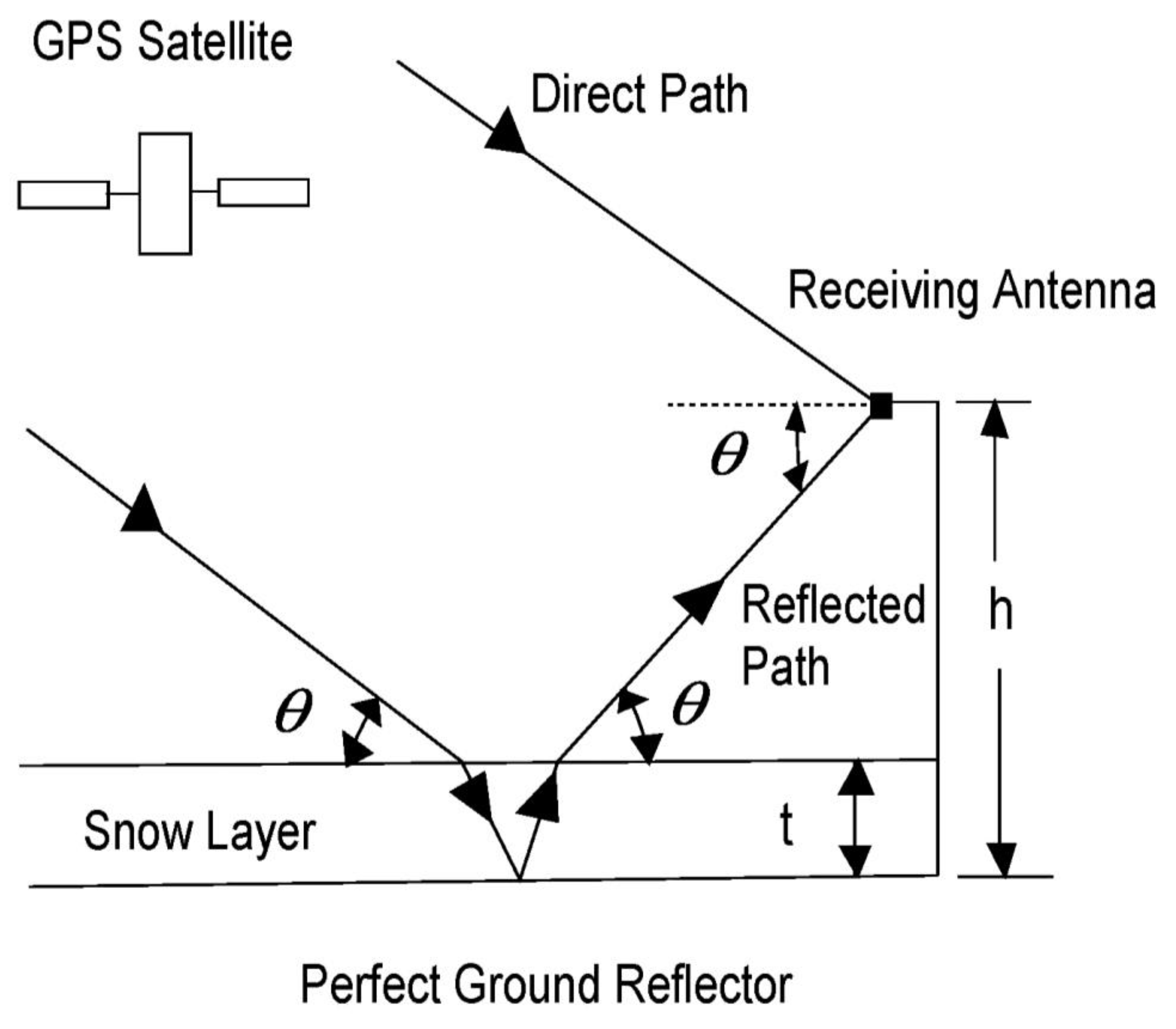
Figure 1 illustrates the total field received by the GPS antenna. The total field is the sum of the direct and specularly-reflected signals. Reflected signals arrive at GPS receivers either coherently or incoherently depending on the roughness of the surface. Coherently reflected signals are caused by smooth surfaces and are called specularly-reflected signals. Most of the reflected signal occurs within the first Fresnel zone about the specular point. In contrast, incoherent reflected signals are caused by rough surfaces and are called diffusely scattered signals.
A vertically-mounted antenna, with the maximum of the main lobe in the horizontal direction (elevation angle of 0°), is chosen to provide equal antenna gain from the directions of the direct and reflected GPS signals. The active Trimble antenna (50.5 mm
42.0 mm
13.8 mm) consists of a microstrip patch antenna, a preamplifier, a radome and a ground plane. The calculation of the total field is simplified with equal antenna gains for the direct and reflected signals. With a vertically-mounted antenna, the received GPS signal strength increases with decreasing elevation angle because the actual antenna gain pattern increases with decreasing elevation angle. In fact, the measured half-power beamwidth of the antenna is approximately 120°. In addition, the antenna gain decreases by approximately 10 dB at 90° away from the maximum of the main lobe. These low elevation angles provide the greatest effect on the reflected signals because the electrical path length of the GPS signal in the snow increases as the elevation angle decreases. As a practical matter, snow or ice accumulation on top of a vertically-mounted antenna will be less than a horizontally-mounted antenna (maximum of the main lobe in the zenith direction) because there is less antenna surface area exposed to the zenith direction. The disadvantage of a vertically-mounted antenna is that ground-based operational GPS antennas are always pointed to zenith (
i.e., antenna is horizontally-mounted). Zenith-pointing antennas maximize the number of viewable GPS satellites and also minimize multipath effects. This paper however uses a vertically-mounted antenna for the reasons given above. Therefore, the relative received power at the right-hand circularly polarized antenna [
24] is
where
rh is the field reflection at horizontal polarization;
rv is the field reflection at vertical polarization;
is the phase shift difference in physical path length between the direct and reflected paths [
25];
is the definition of
i;
h is the height of antenna above conducting surface (m);
t is the snow layer thickness (m);
is the elevation angle (degrees);
m/s is the speed of light in a vacuum;
GHz is the GPS L1 frequency; and
m is the GPS L1 free-space wavelength.
Figure 1.
Geometry of the total GPS L1 signal at the receiving antenna with a height h above a perfect ground reflector. Snow layer has a thickness of t. The elevation angle is given by .
Figure 1.
Geometry of the total GPS L1 signal at the receiving antenna with a height h above a perfect ground reflector. Snow layer has a thickness of t. The elevation angle is given by .
With this model, we compute
rh and
rv by using a ray diagram [
5]
where
is the relative complex permittivity of dry snow. The relative complex permittivity value of dry snow is computed from Tiuri’s microwave dry snow model [
26]
where
is the relative density of dry snow in g cm
−3; and
T is the temperature of snow in degrees C.
The measured data from a snow-covered reflector [
5] are fitted with the above fitting function
P in a QNA.
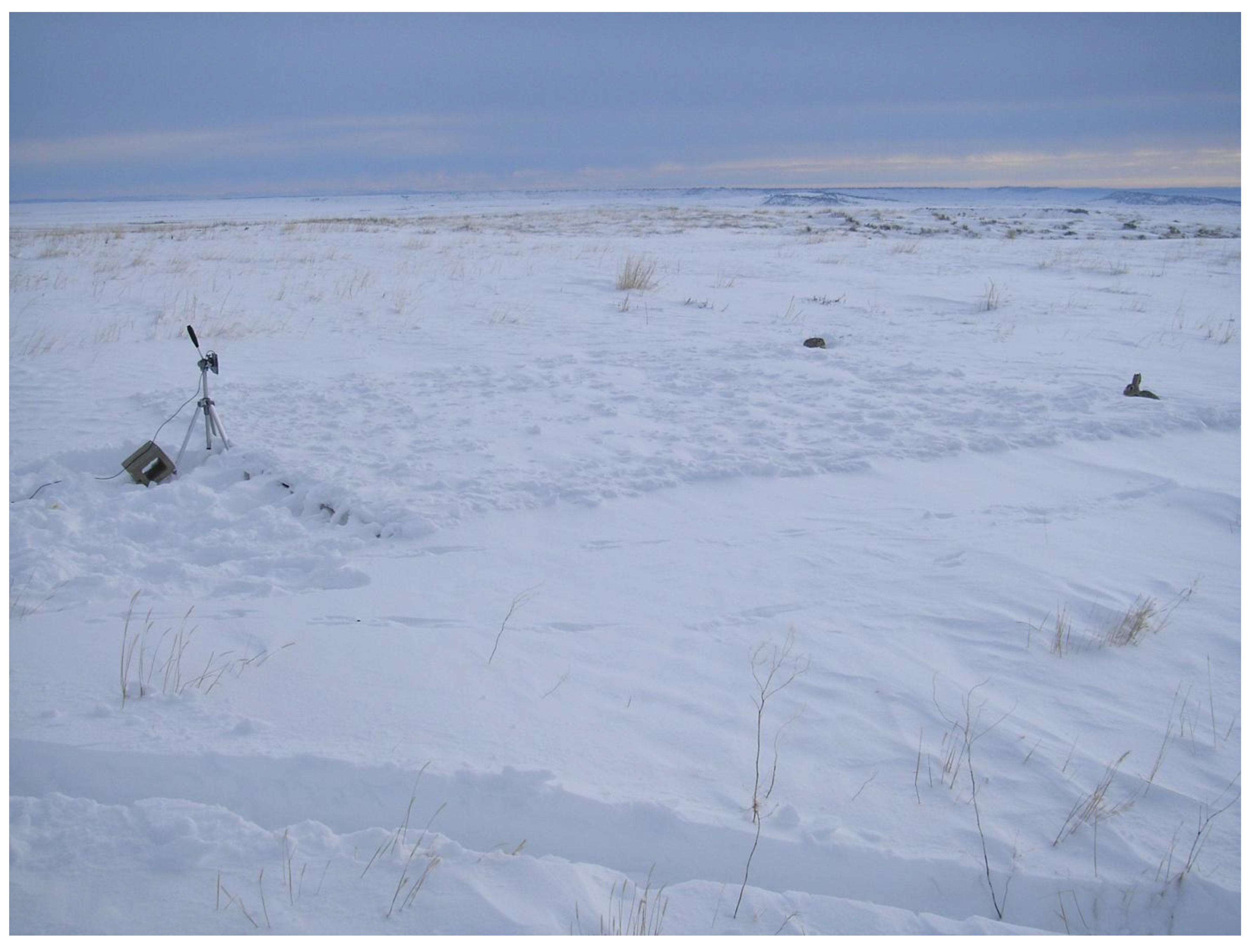
Figure 2 is a photograph of the snow-covered ground reflector used in this experiment. The aluminum ground reflector has dimensions of approximately 5 m
5 m. The ground reflector consists of sixteen 1.22 m
1.22 m plywood sections covered by heavy duty aluminum foil. This ground reflector was screwed into twenty-seven 10.2 cm
10.2 cm
1.83 m plastic fence posts. This provided a reasonably flat surface for the ground reflector. The antenna was mounted on a tripod at the middle of one edge of the ground reflector. Therefore the antenna’s beam illuminated the entire ground reflector. The site was located in terrain that minimized blockage and shadowing. Signal power levels in both measurements and simulation results have been normalized. Power levels were directly recorded in decibels (dB) from the GPS receiver every 0.5 seconds to a laptop computer.
The site was located 13 km west of Billings, MT. The measurements were performed on March 31, 2007 with partly cloudy skies between 14:44 and 15:52 GPS time for satellite PRN 4. The wind-blown snow layer was from a two-day storm that occurred on March 28 and 30, 2007. The snow depth was approximately 7.6 cm
2.5 cm. The snow depth on the ground reflector was measured with a ruler approximately every 2.5 m with one corner as the origin, see
Table 1. The snow temperature increased from −3.3 °C to 0.0 °C during this time. Therefore, an average snow temperature of −1.7 °C was chosen for the model. For this paper, the elevation angles were restricted to be between 5° and 30° in order to maximize the multipath effects from the snow layer. This occurs because the electrical path length of the GPS signal through the snow increases as the elevation angle decreases. This elevation range is similar to that chosen by Larson
et al. [
4]. This elevation angle range yields 8,168 data points.
The antenna was mounted on a tripod above the air-snow interface at a height of approximately 38.3 cm (for
t = 6.8 cm and
h = 45.1 cm). Since this is just several wavelengths away from the ground reflector (
i.e., in the near field of the receiving antenna), the area that contributes into reflection might be somewhat larger. Although the geometric optics approximation may be marginal for this situation, we use it as a first-order estimate. Further studies will assess the accuracy of this method. With this in mind, we use the far field (Fraunhofer diffraction), first Fresnel zone dimensions for estimating the effectiveness of the ground reflector dimensions. With an antenna height of 38.3 cm and an elevation angle of 15°, the first Fresnel zone [
26] is calculated to have a major axis length of approximately 5 m and a minor axis length of approximately 1.5 m. Therefore, the first Fresnel zone lies entirely on the snow-covered reflector for elevations angles ≥ 15°. On the other hand, at an elevation angle of 5° (lowest elevation angle in the measurements), the first Fresnel zone is calculated to have a major axis length of approximately 34 m and a minor axis length of approximately 3 m. Therefore, the first Fresnel zone lies on both the snow-covered reflector and the snow-covered frozen ground for elevations angles < 15°. This indicates that the ground reflector is not large enough for the smaller elevation angles. The measurements indicate that this is not a severe problem. The reflector size design was chosen because of money, time and labor constraints.
Figure 2.
Snow-covered ground reflector. The antenna is mounted vertically on the tripod with h = 45.1 cm.
Figure 2.
Snow-covered ground reflector. The antenna is mounted vertically on the tripod with h = 45.1 cm.
Table 1.
Nine snow depth (t) measurements taken from the base of the ground reflector using a ruler. One corner location is assigned the origin value of (0, 0) in (m). The measured snow depth range is 7.6 cm ± 2.5 cm.
Table 1.
Nine snow depth (t) measurements taken from the base of the ground reflector using a ruler. One corner location is assigned the origin value of (0, 0) in (m). The measured snow depth range is 7.6 cm ± 2.5 cm.
| x, y (m) | (0, 0) | (0, 2.5) | (0, 5) | (2.5, 0) | (2.5,2.5) | (2.5, 5) | (5, 0) | (5, 2.5) | (5, 5) |
| t (cm) | 7.0 | 7.3 | 5.1 | 8.5 | 9.4 | 10.1 | 6.4 | 5.7 | 9.1 |
In order to utilize a QNA efficiently in finding estimates of snow depth and density, we approximate the relative complex permittivity value of dry snow as [
26]
because
The snow depth and the approximate dry snow permittivity value are used as the two inputs to the fitting function P in a QNA. Notice the simple linear relationship in (9) between snow permittivity and snow density. The following snow depth and permittivity values are chosen to bracket the measured and typical values of this experiment. The following 9 snow depth values (t) are used as QNA inputs: 2.54, 5.1, 7.6, 10.1, 20.0, 30.0, 40.0, 50.0, and 100.0 cm. In addition, the following 5 snow permittivity values (εsnow) are used as QNA inputs: 1.3, 1.38, 1.48, 1.68, and 1.80. These values produce 45 different paired combinations of snow depth and snow permittivity.
Each pair of snow depth and permittivity value is used as an input to a QNA. The output of a QNA produces a snow depth, a permittivity value and a standard error (SE) by performing a nonlinear least squares fit between theory and measurement. The process for calculating the SE for each output pair of QNA is given by the following expression
where
y is the measured power value in dB,
P is the fitting function in dB,
t is the snow depth in m, ε
snow is the snow permittivity value, θ is the elevation angle in degrees,
n is the number of data points (8168), and
min is the abbreviation for minimize.
This procedure is performed for all 45 paired combinations. The best estimate of snow depth and permittivity (density) is determined by which QNA output produces the smallest SE.
Table 2 is a summary of the paired input combinations and corresponding output results. A snow depth of 6.8 cm and a snow density of 0.30 g cm
−3 produces the smallest SE of 1.146 dB; the resulting SWE = 2.04 g cm
−2 = 20.4 kg m
−2. This output pair value occurs about 30% of the time (the most frequent output pair) and is shown in bold in
Table 2. This inferred snow depth of 6.8 cm is within the measured depth range of 7.6 cm
2.5 cm. Furthermore, the inferred snow density of 0.30 g cm
-3 is typical for this region at this time of year (0.20–0.40 g cm
−3) [
4,
27,
28]; unfortunately, no snow density measurements were taken.
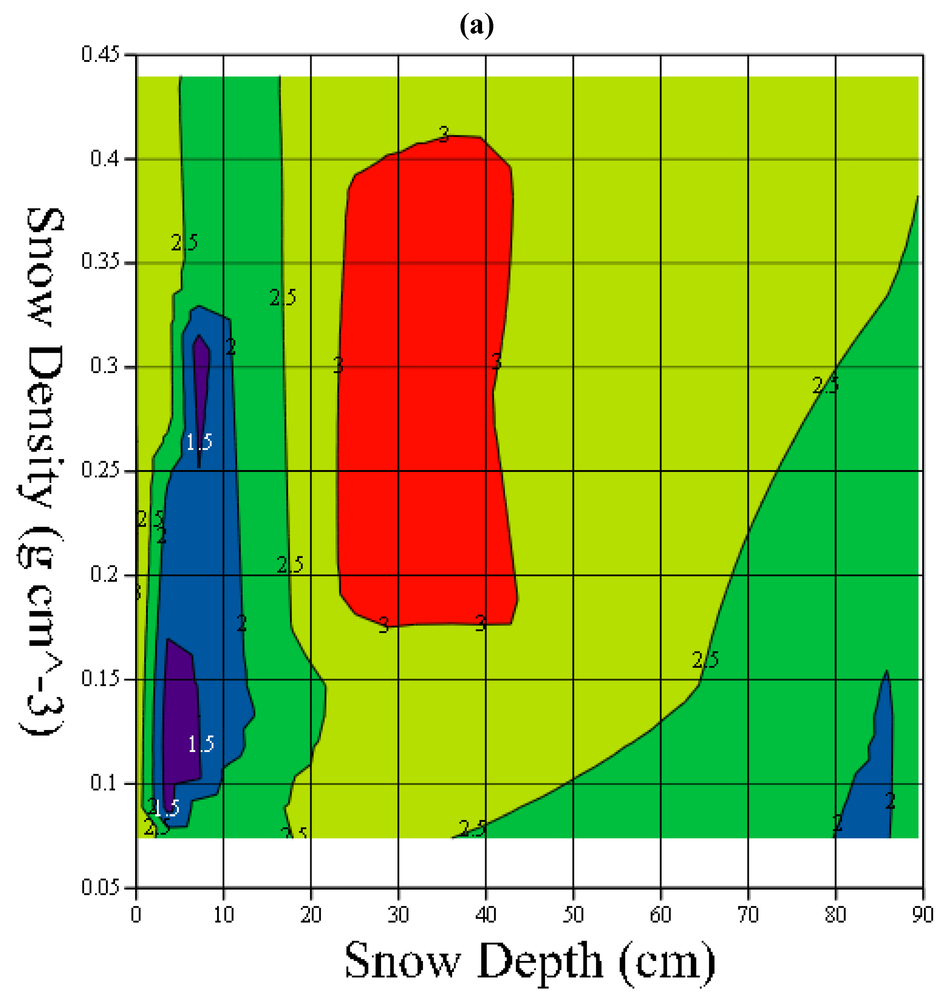
Figure 3 shows two-dimensional contour plots of the QNA output values produced by the 45 input pairs.
Table 2.
Summary of the output values of snow depth (t), snow permittivity (εsnow), snow density (ρd) and standard error (SE) produced by 45 paired input combinations of snow depth and permittivity using a quasi-Newton algorithm (QNA). The bold entries indicate the smallest SE result of 1.146, which corresponds to output values of snow depth and snow density of 6.8 cm and 0.3 g cm−3, respectively.
| INPUT | OUTPUT |
|---|
| t (cm) | εsnow | t (cm) | εsnow | ρd (g cm−3) | SE (dB) |
|---|
| 2.54 | 1.3 | 3.53 | 1.3 | 0.15 | 1.378 |
| 2.54 | 1.38 | 3.56 | 1.4 | 0.13 | 1.277 |
| 2.54 | 1.48 | 3.53 | 1.3 | 0.15 | 1.378 |
| 2.54 | 1.68 | 3.53 | 1.3 | 0.15 | 1.378 |
| 2.54 | 1.8 | 3.53 | 1.3 | 0.15 | 1.378 |
| 5.1 | 1.3 | 3.53 | 1.3 | 0.15 | 1.378 |
| 5.1 | 1.38 | 3.53 | 1.3 | 0.15 | 1.378 |
| 5.1 | 1.48 | 3.8 | 1.27 | 0.083 | 1.161 |
| 5.1 | 1.68 | 6.8 | 1.6 | 0.3 | 1.146 |
| 5.1 | 1.8 | 6.8 | 1.6 | 0.3 | 1.146 |
| 7.6 | 1.3 | 6.8 | 1.6 | 0.3 | 1.146 |
| 7.6 | 1.38 | 6.8 | 1.6 | 0.3 | 1.146 |
| 7.6 | 1.48 | 6.8 | 1.6 | 0.3 | 1.146 |
| 7.6 | 1.68 | 6.8 | 1.6 | 0.3 | 1.146 |
| 7.6 | 1.8 | 6.8 | 1.6 | 0.3 | 1.146 |
| 10.1 | 1.3 | 6.8 | 1.6 | 0.3 | 1.146 |
| 10.1 | 1.38 | 6.8 | 1.6 | 0.3 | 1.146 |
| 10.1 | 1.48 | 3.4 | 1.3 | 0.13 | 1.334 |
| 10.1 | 1.68 | 3.5 | 1.26 | 0.13 | 1.28 |
| 10.1 | 1.8 | 3.4 | 1.27 | 0.13 | 1.334 |
| 20.0 | 1.3 | 0 | 1.15 | 0.08 | 2.752 |
| 20.0 | 1.38 | 0 | 1.42 | 0.21 | 3.051 |
| 20.0 | 1.48 | 3.4 | 1.28 | 0.14 | 1.349 |
| 20.0 | 1.68 | 0.04 | 1.63 | 0.11 | 1.261 |
| 20.0 | 1.8 | 3.8 | 1.28 | 0.14 | 1.351 |
| 30.0 | 1.3 | 2.4 | 1.15 | 0.074 | 2.411 |
| 30.0 | 1.38 | 11.0 | 1.8 | 0.4 | 2.105 |
| 30.0 | 1.48 | 3.4 | 1.28 | 0.14 | 1.349 |
| 30.0 | 1.68 | 6.8 | 1.6 | 0.3 | 1.146 |
| 30.0 | 1.8 | 6.8 | 1.6 | 0.3 | 1.146 |
| 40.0 | 1.3 | 27.6 | 1.39 | 0.2 | 3.426 |
| 40.0 | 1.38 | 26.8 | 1.72 | 0.36 | 3.195 |
| 40.0 | 1.48 | 10.5 | 1.8 | 0.4 | 2.105 |
| 40.0 | 1.68 | 10.5 | 1.8 | 0.4 | 2.105 |
| 40.0 | 1.8 | 6.8 | 1.6 | 0.3 | 1.146 |
| 50.0 | 1.3 | 50.4 | 1.3 | 0.15 | 2.845 |
| 50.0 | 1.38 | 3.53 | 1.3 | 0.15 | 1.378 |
| 50.0 | 1.48 | 52.9 | 1.5 | 0.25 | 2.8 |
| 50.0 | 1.68 | 11.0 | 1.8 | 0.4 | 2.105 |
| 50.0 | 1.8 | 6.8 | 1.6 | 0.3 | 1.146 |
| 100.0 | 1.3 | 86.5 | 1.3 | 0.15 | 1.972 |
| 100.0 | 1.38 | 3.73 | 1.27 | 0.14 | 1.307 |
| 100.0 | 1.48 | 3.53 | 1.3 | 0.15 | 1.378 |
| 100.0 | 1.68 | 88.2 | 1.87 | 0.44 | 2.761 |
| 100.0 | 1.8 | 89.4 | 1.8 | 0.4 | 2.535 |
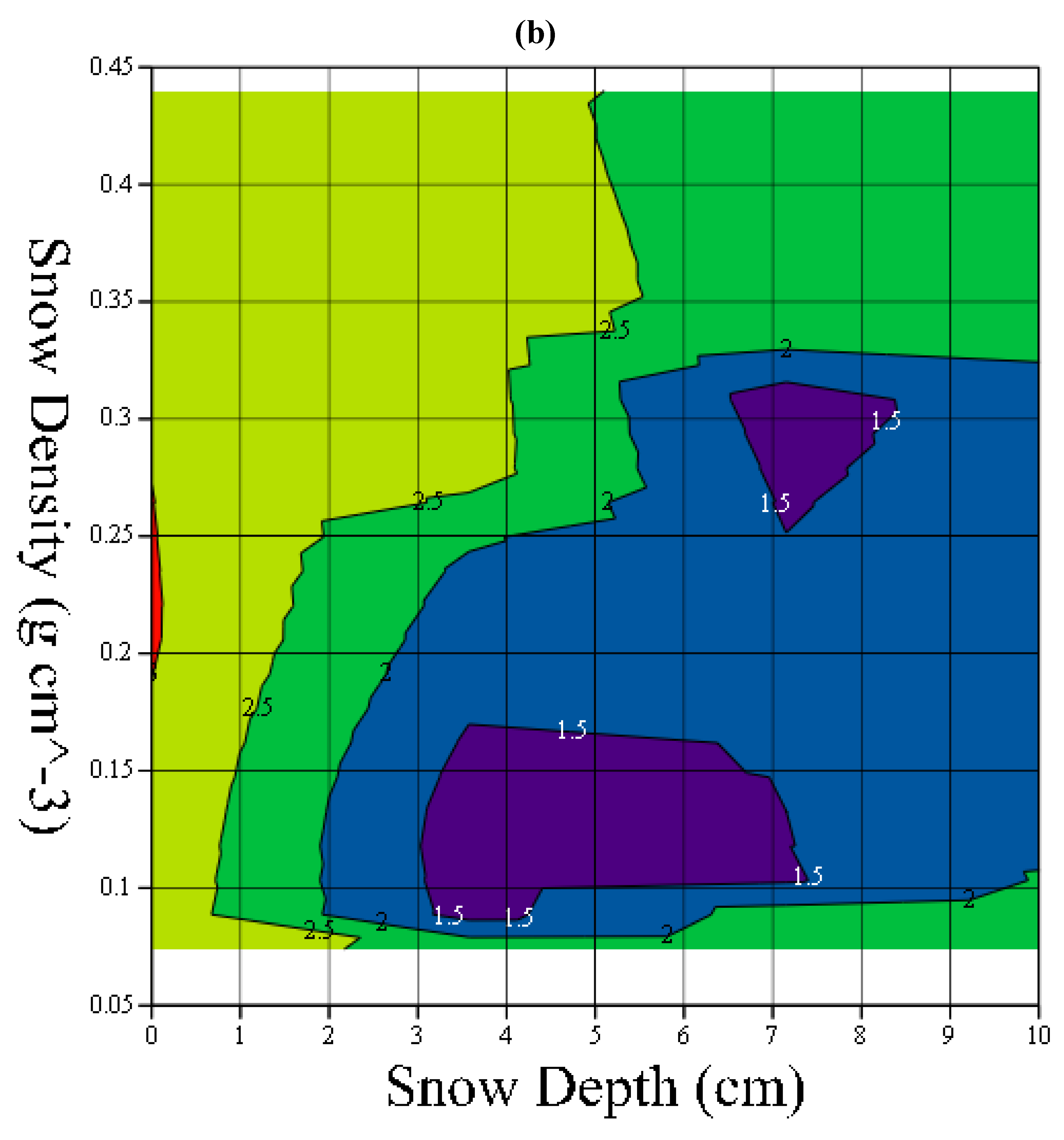
Figure 3.
(a) Two-dimensional contour plot of snow depth (
t) and snow density (
ρd) with contour values of standard error (SE) of the QNA output values produced by the 45 input pair combinations of snow depth and permittivity (ε
snow) in
Table 2 using a quasi-Newton algorithm (QNA). The purple regions show the smallest SE.
(b) Expanded view of
(a) for output snow depths between 0 and 10 cm.
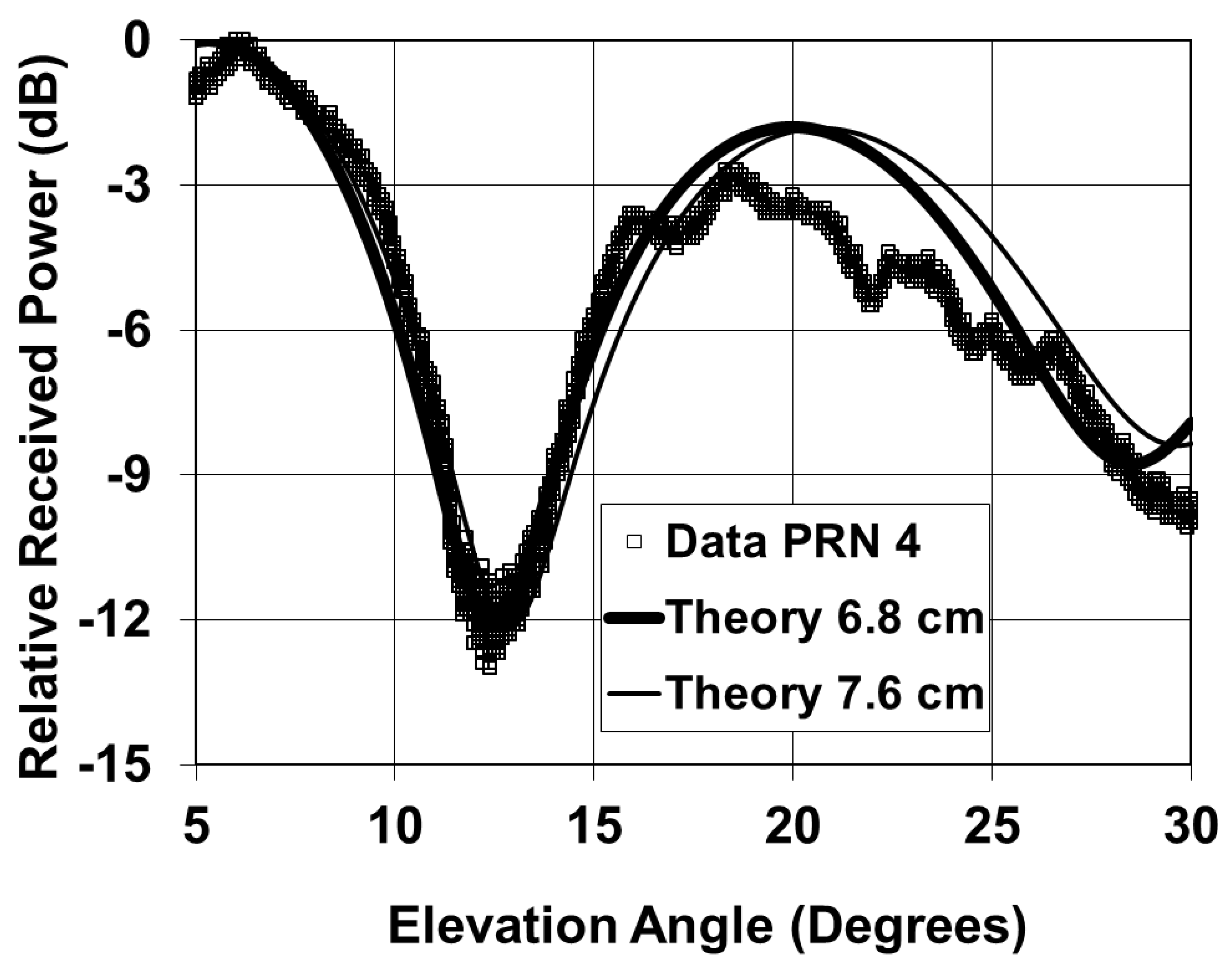
Figure 4 shows the measurement and theoretical results for 6.8- and 7.6-cm-thick snow layers. The 7.6-cm-thick snow layer was used as the best fit to the data in [
5], and is shown here for comparison purposes. The snow densities for the 6.8- and 7.6-cm-thick snow layers are 0.30 and 0.24 g cm
−3, respectively. The corresponding relative permittivity values [
26] for the 6.8- and 7.6-cm-thick snow layers are
εsnow = 1.60 –
i3.58 × 10
−4 and
εsnow = 1.48 –
i2.76 × 10
−4, respectively. The results shown here provide evidence that estimates of snow depth and density (and therefore SWE) may be possible using GPS multipath signals. However, it should be noted that this technique requires several input guess values for snow depth and permittivity (density) to determine which output pair produces the minimum SE.
Figure 4.
(Lines) Theoretical and (square) measured elevation plots for a ground reflector covered by 6.8- and 7.6-cm-thick snow layers with h = 45.1 cm for the GPS satellite PRN 4. The values εsnow = 1.60 – i3.58 × 10−4 and εsnow = 1.48 – i2.76 × 10−4 are used in the 6.8- and 7.6-cm-thick snow layer models, respectively. The GPS times from the measurements are 14:44 to 15:52.
2.2. Without a Ground Reflector
The possibility of using GPS signals to estimate SWE is investigated further by replacing the perfect ground reflector with smooth, flat frozen soil. This situation was considered in experiments [
4] where, unlike here, a commonly used horizontally-mounted GPS antenna was employed. The relative received power (
P) at a GPS antenna for a snow-covered frozen soil model is computed by using the model described in [
6]. The total field is the sum of the direct and specularly-reflected signals. The relative received power at the right-hand circularly polarized antenna is given in (1). The dielectric identifier,
j, has the following values in this model: 1 for the snow layer and 2 for the frozen soil. The field reflection is
where
where
is the relative complex permittivity of dry snow or frozen soil, and
t is the dry snow layer thickness (m).
We model the relative complex permittivity value of the frozen soil with a constant profile for two different frozen soils given in Hallikainen
et al. [
29]. In particular, the two different frozen soil graphs, Fields 1 and 5 at −11 °C, are extrapolated to the GPS L1 frequency to yield the following approximate relative complex permittivity values:
ε2 =
εsoil 1 = 5 −
i0.5 for Field 1 and
ε2 =
εsoil 5 = 10 −
i2.0 for Field 5. The frozen soil characteristics of Fields 1 and 5 are shown in
Table 3. A more realistic model of the frozen soil [
30] should be implemented for future studies.
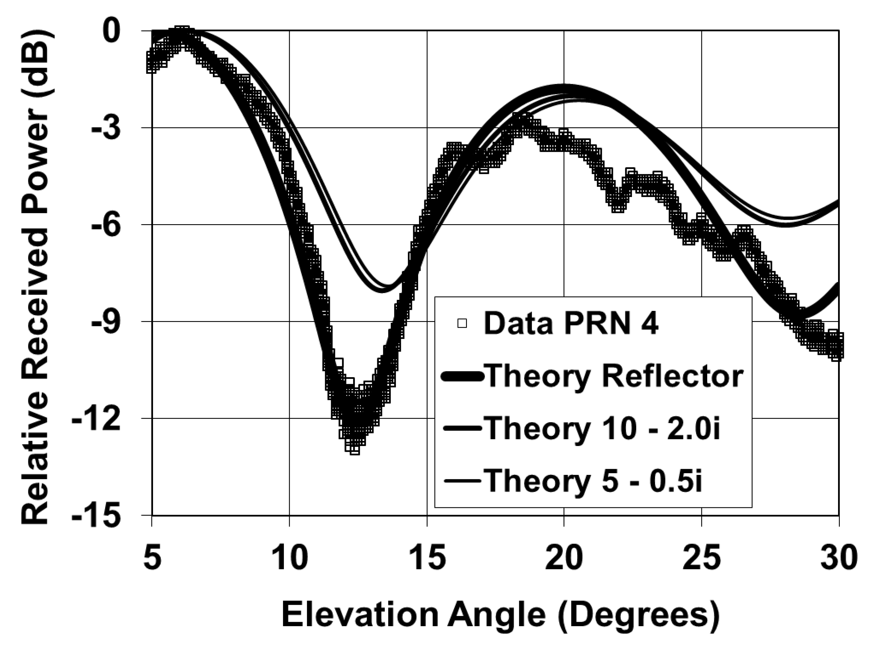
Figure 5 shows the measurement and theoretical results for the perfect reflector and the two frozen soils. The frozen soils reduce the fade depths as compared to the perfect reflector. In addition, the frozen soils increases the elevation angle values at the first fade depth as compared to the perfect reflector. With these results, a QNA technique might prove useful in estimating SWE for snow-covered frozen soil. In order to implement a QNA, an appropriate snow depth guess value could be obtained by the method outlined by Larson
et al. [
4]. The other guess value, snow density, could be found by using a snow density typical of the region and season. Several other snow depth and density (permittivity) pairs could be selected that would bracket this initial input guess pair value. The SE results from the different paired values may provide an estimate of the SWE.
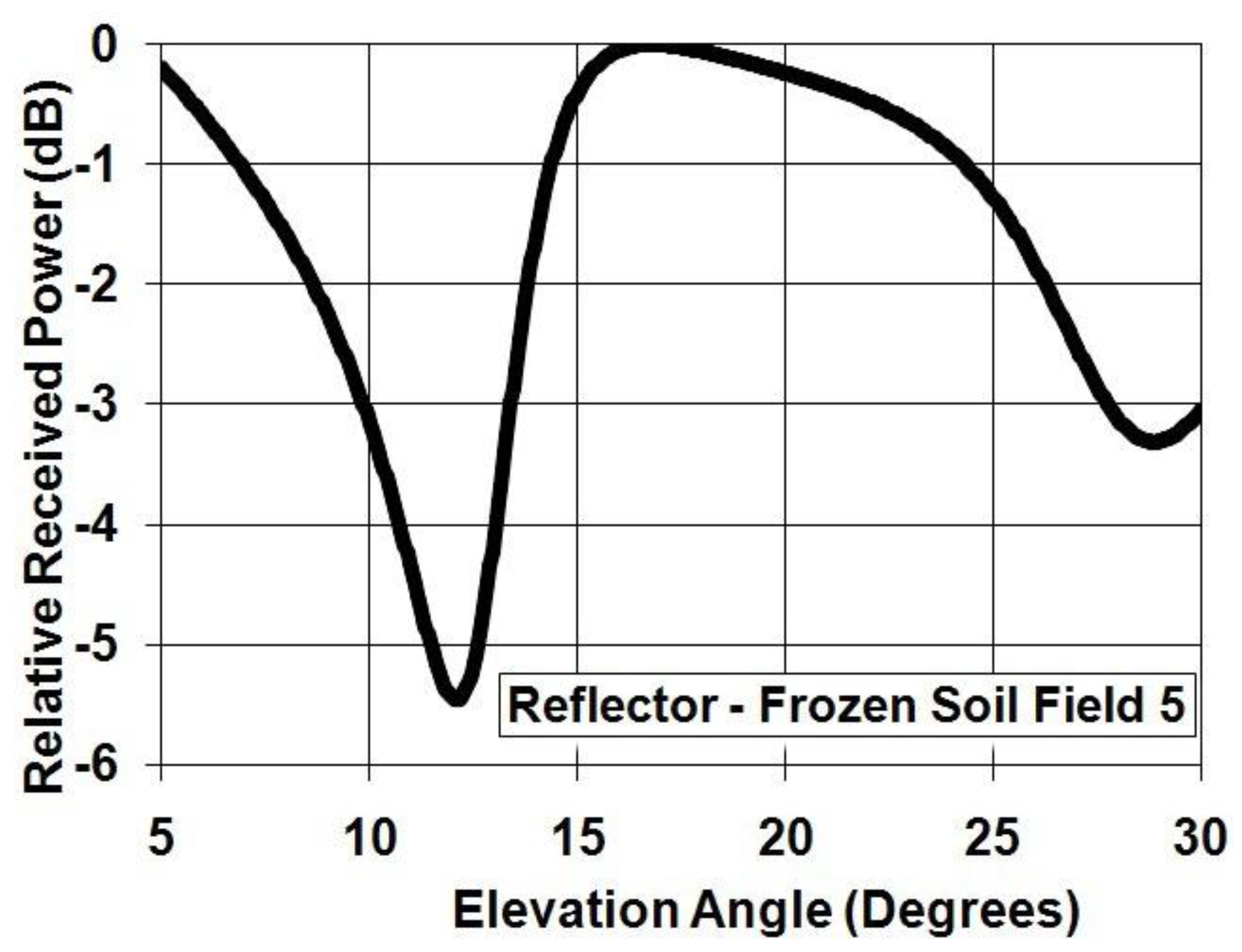
Figure 6 shows the power difference results between the snow-covered perfect reflector and the snow-covered frozen soil from Field 5. The results from this difference plot could possibly be used to estimate the permittivity of the frozen soil under the reflector.
Table 3.
Frozen soil characteristics of Fields 1 and 5 as given in [
29].
Table 3.
Frozen soil characteristics of Fields 1 and 5 as given in [29].
| | Sand (%) | Silt (%) | Clay (%) | Volumetric Wetness (cm3 cm−3) | Bulk Density (g cm−3) |
|---|
| Field 1 | 51.5 | 35.1 | 13.4 | 0.24 | 1.54 |
| Field 5 | 5 | 47.6 | 47.4 | 0.36 | 1.42 |
Figure 5.
(Lines) Theoretical and (square) measured elevation plots for a 6.8-cm-thick snow layer covering a ground reflector and two types of frozen soil with
h = 45.1 cm for the GPS satellite PRN 4. The soil characteristics are given in
Table 3. The values
εsnow = 1.60 −
i3.58 × 10
−4,
εsoil1 = 5 −
i0.5 and
εsoil5 = 10 −
i2.0 are used in the model. The GPS times from the measurements are 14:44 to 15:52.
Figure 6.
Theoretical elevation plot for the difference between a 6.8-cm-thick snow layer covering a ground reflector and a 6.8-cm-thick snow layer covering frozen soil with a composition of Field 5 with h = 45.1 cm. The values εsnow = 1.60 − i3.58 × 10−4 and εsoil5 = 10 − i2.0 are used in the model.


