1. Introduction
The history of urban growth indicates that urban areas are one of most dynamic places on the Earth’s surface. Despite its regional economic importance, urban growth has a considerable impact on the surrounding ecosystem [
1]. Most often, the trend of urban growth is towards the urban-rural-fringe, where there is less built-up area, and access to irrigation and other water management systems. In the last few decades, a substantial growth of urban areas has occurred worldwide. Population increase is one of the most obvious agents responsible for this growth. In 1900, only 14% of the world’s population lived in urban areas, but by 2000, this figure had increased to 47% [
2]. The report also predicts that by 2030, the percentage of the population residing in urban areas will be 60%. Currently, the major environmental concerns that have to be analyzed and monitored carefully, for effective land use management, are those driven by urban growth.
Effective analysis and monitoring of land cover changes require a substantial amount of data about the Earth’s surface. This is most widely achieved by using remote sensing (RS) tools. Remote sensing provides an excellent source of data, from which updated land use/land cover (LULC) information and changes can be extracted, analyzed, and simulated efficiently. LULC mapping, derived from remotely sensed data, has long been an area of focus for various researchers [
3]; recent advances in Geographic information systems (GIS) and RS tools and methods enable researchers to model urban growth effectively. Cellular Automata (CA) constitutes a possible approach to urban growth modeling by simulating spatial processes as discrete and dynamic systems in space and time that operate on a uniform grid-based space [
4,
5]. The ability of CA to represent complex systems with spatio-temporal behavior, from a small set of simple rules and states, makes it suitable for modeling and investigating urban environments [
4]. Planning activities may also benefit from CA; CA enables the understanding of the urbanization phenomenon and the exploration of
what-if scenarios.
In this study, an integrated approach incorporating GIS, RS, and modeling is applied to identify and analyze patterns of urban changes within the Setúbal and Sesimbra municipalities between the years 1990 and 2006. The study also aims to determine the probable future developed areas so as to enable the anticipation of planning policies that aim to preserve the unique natural characteristics of the study area.
2. Study Area
The study focuses on two administrative areas, Setúbal and Sesimbra, in the Lisbon Metropolitan Area (AML), Portugal (
Figure 1).
The AML has experienced considerable population growth in two distinct phases: the rural to urban migration, which took place from 1940 to 1960, and the return of thousands of Portuguese from the overseas ex-colonies in the 1970s [
6,
7]. These phases significantly affected the rate of urban sprawl in the area and led to a current population in the AML of approximately 2.6 million. The population is constrained within an area of 2,957.4 km
2 [
8], and represents nearly 25% of the Portuguese population. One of Portugal’s nature reserves, the Serra da Arrábida, is found within the study area, and due to its location near the coast, it attracts various human activities that result in losses of farmland, forest cover, and depleted water resources. The Portuguese government has created several protected areas to reduce and control building speculations and to protect the natural heritage [
7]. Urban pressure and the impact on the natural resources of this region require consideration and careful assessment for monitoring and planning land management, urban development, and decision-making.
Figure 1.
Location of the study area: two administrative areas, Setúbal and Sesimbra, in the Lisbon Metropolitan Area (AML), Portugal.
Figure 1.
Location of the study area: two administrative areas, Setúbal and Sesimbra, in the Lisbon Metropolitan Area (AML), Portugal.
3. Data
Utilized in this study are a national land cover map, with a minimum mapping unit (MMU) of 1 ha, from the Portuguese Geographic Institute (IGP) from the year 1990 (COS 90), a Landsat TM satellite image from the year 2000, and LISS-III (summer) and SPOT (spring) satellite images from the year 2006. Land cover maps with an MMU of 1 ha, from the years 2000 and 2006, were derived from Landsat TM (acquired on August 24, 2000), LISS-III (acquired on August 1, 2006), and SPOT (acquired on May 24, 2006) images. The spring and summer images for 2006 were used to better distinguish some of the land cover classes (e.g., irrigated and non-irrigated agriculture). Furthermore, ancillary data, such as a digital elevation model (DEM), major road networks, and high spatial resolution aerial photographs were integrated into the analyses.
4. Methods
4.1. Pre-Processing and Land Cover Schemes
The satellite images used in this study were ortho-rectified by the European Space Agency (ESA) within the frame of the project, IMAGE2006 [
9]. Positional accuracy was very good and is expressed with a root mean square error of less than 1 pixel. As a pre-processing phase, individual bands were extracted for further processing and analysis to cover the entire study area. Two scenes of spring images for the year 2006 were spliced together on a band by band basis because no single scene covered the entire study area. The datasets were provided along with a 44 land cover class legend. For the sake of simplicity, the 44 classes were aggregated into seven major classes, as shown in
Table 1.
Table 1.
Land cover classes used in the study.
Table 1.
Land cover classes used in the study.
| Land cover classes | Descriptions based on the CORINE land cover classes |
|---|
| Built-up areas | All forms of urban fabrics and urban related features |
| Urban vegetation | Urban vegetation or urban parks, or both |
| Non-irrigated | Annual and permanent crops, complex cultivation patterns, and agriculture with natural vegetation |
| Irrigated land | Permanently irrigated land, rice fields, and fruit plantations |
| Forest cover | Deciduous, coniferous, mixed forest, and transitional woodland/shrub |
| Bare land | Sand plains and dunes, and bare rock |
| Water bodies | Water courses, water bodies, estuaries, and salt marshes |
4.2. Land Cover Classification and Accuracy Assessment
The advent of satellite data in the last few decades opened up a new dimension for the generation of land cover information. While the extraction of such information is possible using the ‘traditional’ approaches of surveying or digitizing, land cover information extraction that is based on image classification has attracted the attention of many remote sensing researchers [
10]. The latter is now considered the ‘standard’ approach [
11]. In various empirical studies, different classification techniques have been discussed and they can be categorized as being either supervised or un-supervised; parametric or non-parametric; hard or soft classifiers [
10]. All classifiers have limitations, but alternative methods can be suggested to deal with those limitations. A supervised pixel-based technique is, for example, criticized for producing inconsistent “salt and pepper” output. An alternative object-oriented technique has been suggested for a better and more cohesive classification result. This is because the world is not “pixelated”; rather it is arranged in objects [
12]. Such object-based classifiers are essential for urban land change studies [
13] because of the heterogeneous nature of urban areas.
We utilized eCognition software, an object-oriented image analysis program, to classify the satellite images. Land cover classification in eCognition is based on the process of image segmentation, where pixels are merged into objects based on the pixel’s spectral properties and the defined scale parameters. Scale parameters refer to the average size of image objects. The segmentation process stops when the image objects exceeds a user-defined threshold [
14]. Image segmentation in eCognition requires some parameters to be set: (1)
image layer weights: indicate the importance of a layer; (2)
scale parameter; (3)
color: determines the homogeneity of the image; and (4)
shape: controls the degree of object shape homogeneity. There is no specific guideline on the rules to be set and these parameters are often set in a trial and error mode. In this case, all the image layers were considered and given equal importance (
i.e., 1). Additionally, different scale parameters, based on visual analysis of segmentation results, were attempted. Once the segmentation process was done, classification was implemented using a resource-based sample collection and a standard nearest neighbor algorithm. Based on these procedures, land cover maps for the years 2000 and 2006 were generated.
Accuracy assessment, which is an integral part of any image classification process, was calculated to estimate the accuracy of the land cover classifications. A confusion matrix is the common way of representing classification; this has been recommended and adopted as the standard reporting convention [
15]. In this paper, accuracy assessment was achieved using a high spatial resolution (50 cm) aerial photograph as reference. A set of reference points (240 stratified random points) were generated for each derived map. These points were verified and labeled against the reference data. The overall user’s and producer’s accuracies were calculated from the matrices. The Kappa coefficient, [
16], which is one of the most popular measures of addressing the difference between actual agreement and chance agreement, was also computed.
4.3. Landscape Metrics and Urban Sprawl Measurement
4.3.1. Landscape Metrics
Changes in urban structures can be described using information obtained from spatial metrics, which are algorithms used to describe and quantify the spatial characteristics of patches, class areas, and the entire landscape [
17,
18]. The changes in urban landscape were measured and analyzed using the FRAGSTATS tool and thematic maps that represent both built-up and non-built-up patches. In this paper, seven spatial metrics (CA, NP, ED, LPI, EMN_MN, FRAC_AM, and Contagion) were used for analyzing urban land cover changes (
Table 2). The selection of the metrics was based on their simplicity and effectiveness in depicting urban forms evolution, as demonstrated in previous researches [
17,
18,
19,
20,
21].
Table 2.
Spatial metrics used in the study.
Table 2.
Spatial metrics used in the study.
| Metrics | Description | Units | Range |
|---|
| CA-Class Area | CA measures total areas of built-up and non-built-up areas in the landscape in hectares | Hectares | CA>0, no limit |
| NP-Number of Patches | NP is the number of built-up and non-built-up patches in the landscape | None | NP≥0, no limit |
| ED-Edge Density | ED equals the sum of the lengths (m) of all edge segments involving the patch type, divided by the total landscape area (m2) | Meters per hectare | ED≥0, no limit |
| LPI-Largest Patch Index | LPI percentage of the landscape comprised by the largest patch | Percent | 0<LIP≤100 |
| EMN_MN- Euclidian Mean Nearest Neighbor Distance | Equals the distance (m) to the nearest neighboring patch of the same type, based on the shortest edge-to-edge distance | Meters | EMN_MN>0, no limit |
| FRAC_AM: Area weighted mean patch fractal dimension | Area weighted mean value of the fractal dimension values of all urban patches; the fractal dimension of a patch equals two times the logarithm of patch area (m2), while the perimeter is adjusted to correct for its raster bias | None | 1≤FRAC_AM≤2 |
| Contagion | Describes the heterogeneity of a landscape and measures the extent to which landscapes are aggregated or clumped | Percent | 0<Contagion≤100 |
4.3.2. Urban Sprawl Measurement Using Shannon Entropy
Urban sprawl is a complex phenomenon and has both environmental and social impacts [
22,
23]. It can be caused by population growth, topography, proximity to major resources, services, and infrastructure. Many attempts have been made to measure urban sprawl [
23,
24,
25] by measuring Shannon’s Entropy within a GIS. Shannon’s Entropy is used to measure the degree of spatial concentration and dispersion, as defined by geographical variables [
24,
25,
26]. The entropy value varies from 0 to 1. If the distribution is maximally concentrated in one region, the lowest entropy value (
i.e., 0) is obtained, while an evenly dispersed distribution across space gives a maximum value of 1. In this study, urban sprawl, over a period from 1990 to 2006, was determined by computing built-up areas from land cover maps of the years 1990, 2000, and 2006. Afterwards, Shannon entropy calculations were made. The relative entropy (
En) is given by,
where
and
xi is the density of land development, which equals the amount of built-up land divided by the total amount of land in the
ith of
n total zones. The number of zones, in this paper, refers the number of buffers around the city center. In this study, 15 and 16 km concentric buffer rings around the city centers of the two areas were needed to cover all parts of Setúbal and Sesimbra, respectively.
4.4. Urban Land Use Change Modeling Using CA-Markov
4.4.1. CA-Markov Model Description
This study adopts an existing modeling technique, CA-Markov Chain analysis, embedded in IDRISI Kilimanjaro software from Clarks Labs. A Markov Chain CA integrates two techniques: Markov Chain analysis and CA. The Markov Chain analysis describes the probability of land cover change from one period to another by developing a transition probability matrix between
t1 and
t2. The probabilities may be accurate on a per category basis, but there is no knowledge of the spatial distribution of occurrences within each land cover class [
27]. In order to add the spatial character to the model, CA is integrated into the Markovian approach. The CA component of the CA-Markov model allows the transition probabilities of one pixel to be a function of the neighboring pixels. CA-Markov models the change of several classes of cells by using a Markov transition matrix; a suitability map and a neighborhood filter [
27].
In this study, the Markov Chain analysis model was implemented using the Markov module available in the software. The first step in the model was to develop a transition probability matrix for each of the land cover classes between the years 1990 and 2000, and this in turn was used as an input for modeling land cover change. In addition, two types of criteria (constraints and factors) were developed to determine which lands were to be considered for further development (suitable lands). The constraints were standardized into a Boolean character of 0 and 1, while the factors were standardized to a continuous scale of suitability from 0 (least suitable) to 255 (most suitable). The constraints included water bodies, existing urban areas, and natural parks (
Table 3). These constraints were standardized into continuous variables by applying Sigmoidal, J-shaped, and Linear functions. Details of these fuzzy scaling approaches can be found in [
27]. A transition suitability image collection was created using the suitability maps derived from the two criteria using the scaling approaches. The decision rules used to generate the criteria and factors were based on the legislation defined by [
28].
Table 3.
Boolean approach criteria development.
Table 3.
Boolean approach criteria development.
| Change Drivers | Descriptions |
|---|
| Land cover | Based on the trend of the land cover change; agricultural land and bare lands are considered the two possible land cover types available for development. |
| Distance from roads | Areas within 500 m of major road networks are considered suitable [
29]. Thus, the continuous image of distance from roads was reclassified to a Boolean expression such that areas within 500 m of the road are suitable. |
| Slope | Areas that have low slopes (less than 15%) are suitable for development while areas with greater than 15% slope are not suitable |
| Distance from water bodies | A protection buffer of 50 m from the sea and navigable waters was created and areas within 50 m of the water bodies were considered unsuitable. |
| Distance from built-up areas | Areas close to developed areas are more suitable for urban development than areas far from built-up areas. |
| Distance from protected areas | To preserve the natural park, a protection zone of 50 m is stated in the legislations, and areas within 50 m of the protected areas are considered unsuitable. |
4.4.2. Implementing and Validating the Model
CA analysis was carried out with the CA-Markov module, which uses the output from the above stated Markov Chain analysis and transition suitability image collection, and applies a contiguity filter. The Markov module is based on the first law of Geography by using a contiguity rule [
30]. The rule states that a pixel that is near one specific land cover category (e.g., urban areas) is more likely to become that category than a pixel that is farther. The definition of nearby is determined by a spatial filter that the user specifies. In this study, a contiguity filter of 5 × 5 pixels was applied.
Model validation is an important step in the modeling process although there is no consensus on the criteria to assess the performance of land use change models [
31]. One way to quantify the predictive power of the model is to compare the result of the simulation
t2 (2006) to a reference or “real” map of
t2 (2006) using Kappa variations [
31,
32]: Kappa for no information (
Kno), Kappa for location (
Klocation), and Kappa for quantity (
Kquantity).
Kno indicates the proportion classified correctly relative to the expected proportion classified correctly by a simulation with no ability to specify accurately quantity or location [
31].
Klocation is defined as the success due to a simulation’s ability to specify location divided by the maximum possible success due to a simulation’s ability to specify location perfectly [
31].
Kquantity is a measure of validation of the simulations to predict quantity perfectly. If the predictive power of a model is considered strong (
i.e., greater than 80%), then it will be reasonable to make future projections (
i.e., in this case for year 2020) assuming that the transition mechanism verified between 1990 and 2000 is going to be repeated.
5. Results and Discussions
5.1. Land Cover Classification and Accuracy Assessment
An object-oriented image analysis was applied to derive the LULC maps (
Figure 2). In order to use the derived maps for further change analysis, the errors were evaluated and quantified in terms of classification accuracy (
Table 4 and
Table 5). Overall accuracies for the maps of 2000 and 2006 were, respectively, 92.51% and 87.68%. In [
33], it is noted that a minimum accuracy value of 85% is required for effective and reliable land cover change analysis and modeling. The classification achieved in this study produces an overall accuracy that fulfils the minimum accuracy threshold. However, looking at
Table 4, the user’s and producer’s accuracies of the urban class, which is the class of most interest in this study, provide accuracies of 63.04% and 60.61%, respectively. In other words, only 60.61% of the urban areas have been correctly identified as urban and only 63.04% of the areas classified as urban are actually urban. A more careful look at the error matrix reveals that there is significant confusion in discriminating urban areas from non-irrigated land. The user’s and producer’s accuracies for the urban category in
Table 5 are greater than 85%, which are sensible measures of accuracy. It is important to note that the user’s and producer’s accuracy are sensitive to a number of factors, including the number of random points generated and the sampling method employed. The Kappa coefficient, which is a measure of agreement, can also be used to assess the classification accuracy [
15]. It is not uncommon that the Kappa coefficient appears to be low [
34], giving the impression that the coefficient takes into account not only the actual agreement in the error matrix, but also the chance agreement [
15]. Kappa was calculated to be 0.86 and 0.83 for the land cover maps of 2000 and 2006, respectively.
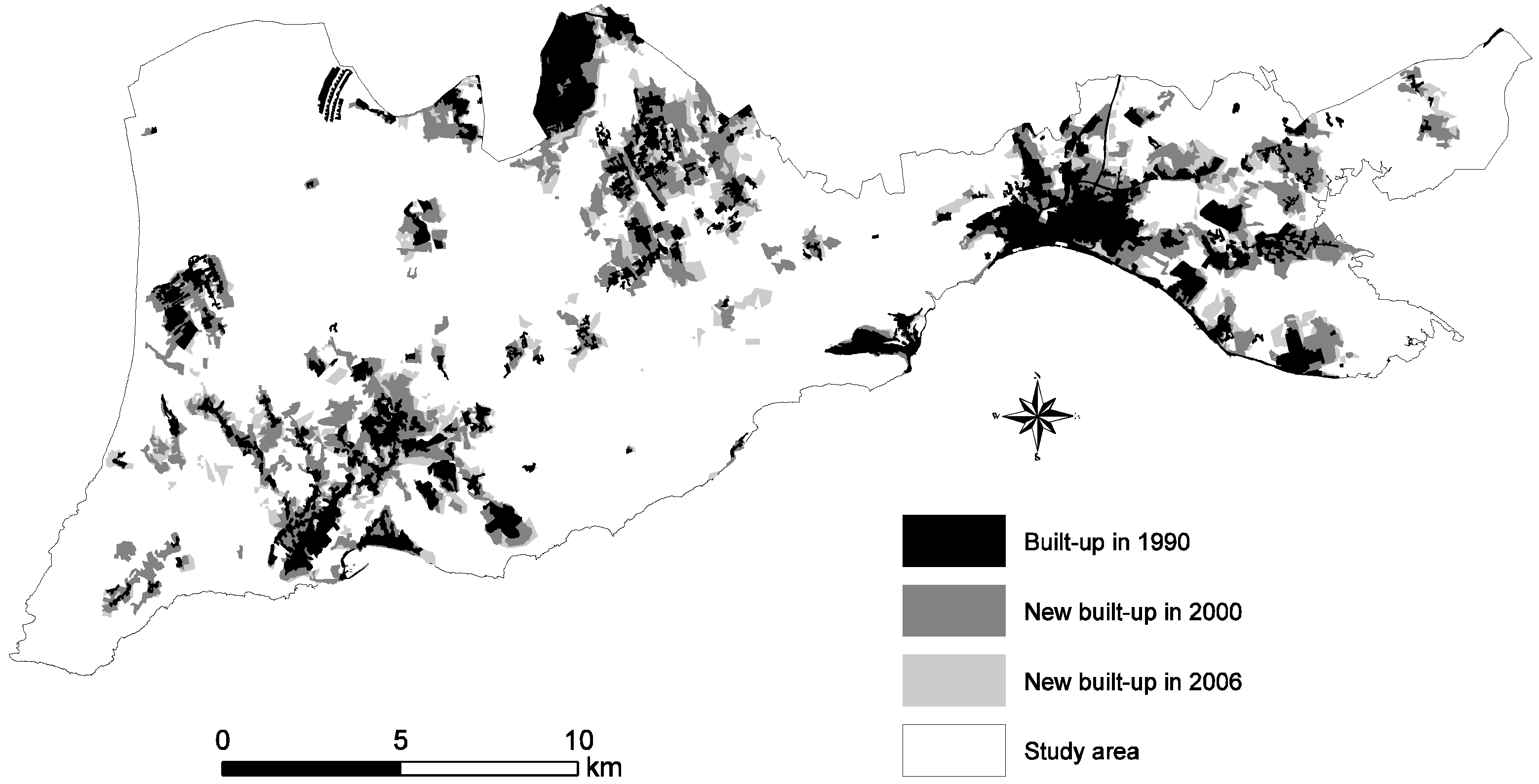
Figure 2.
Urban land cover changes between 1990 and 2006.
Figure 2.
Urban land cover changes between 1990 and 2006.
Table 4.
Error matrix (%): image classification of 2000.
Table 4.
Error matrix (%): image classification of 2000.
| | | Reference map |
|---|
| | | Built-up areas | Urban veg. | Non-irrig. | Irrigated land | Forest cover | Bare land | Water bodes | Total | User’s Accuracy |
|---|
| Classified map | Built-up areas | 29 | | 11 | 3 | 2 | 1 | | 46 | 63.04 |
| Urban veg. | | | | | | | | 0 | - |
| Non-irrig. | 3 | | 126 | | 12 | 3 | | 144 | 87.5 |
| Irrigated land | | | | 32 | 8 | | | 40 | 80 |
| Forest cover | 10 | | 5 | | 530 | | | 545 | 97.25 |
| Bare land | 6 | | | | | 18 | | 24 | 75 |
| Water bodies | | | | | | | 56 | 56 | 100 |
| Total | 48 | 0 | 142 | 35 | 552 | 22 | 56 | 855 | |
| Producer’s accuracy | 60.61 | - | 88.73 | 91.42 | 96.01 | 81.81 | 100 | | |
Table 5.
Error matrix (%): image classification of 2006.
Table 5.
Error matrix (%): image classification of 2006.
| | | Reference Map |
|---|
| | | Built-up areas | Urban veg. | Non-irrig. | Irrigated land | Forest cover | Bare land | Water bodes | Total | User’s Accuracy |
|---|
| Classified map | Built-up areas | 240 | | 30 | | 6 | | | 276 | 86.95 |
| Urban veg. | | | | | | | | 0 | - |
| Non-irrig. | 20 | | 180 | 10 | 10 | | | 230 | 81.81 |
| Irrigated land | | | 8 | 24 | | | | 32 | 75 |
| Forest cover | 2 | | 8 | | 202 | | | 212 | 95.28 |
| Bare land | | | | | | 3 | | 3 | 100 |
| Water bodies | | | 7 | | | | 70 | 77 | 90.1 |
| Total | 262 | 0 | 233 | 34 | 218 | 3 | 70 | 820 | 90.9 |
| Producer’s accuracy | 91.6 | - | 77.25 | 70.59 | 92.66 | 100 | 100 | | |
5.2. Urban Land Use Changes and Urban Sprawl Measurement with Landscape Metrics and Shannon’s Entropy
5.2.1. Analysis of Landscape Metrics
Spatial metrics and their variation were calculated for the built-up areas, which increased by 91.11% between 1990 and 2000 (
Table 6). Similarly, urban growth increased in the period between 2000 and 2006. However, the rate of growth was slower (
i.e., 6.34% for a six year period). Such an increase in urban growth is not uncommon in areas located in a metropolitan city, such as Lisbon. This is associated with the availability of resources, services, infrastructures, and proximity to the coast.
The NP in a landscape analysis indicates the aggregation or disaggregation in the landscape, while LPI measures the proportion of total landscape area comprised by the largest urban patch. The NP (i.e., urban blocks) decreased considerably (51.28%) between 1990 and 2000, and increased by 17.54% between 2000 and 2006. This suggests an urbanization made by agglomeration of pre-existing urban patches in the first period while, in the second period, urbanization was characterized by dispersion. The development of a number of isolated, fragmented, or discontinuous built-up areas occurred in the second period.
LPI increased by 115% between 1990 and 2000, thus indicating considerable growth within the historical urban core. However, this tendency changed in the second period, when the size of the LPI decreased by 25.94%. Although we have a slower urbanization rate in the second period, this one is characterized by the appearance of new, dispersed settlements. ED increased by 26.93% between 1990 and 2000, thus indicating an increase in the total length of the edge of the urban patches, as due to land use fragmentation. FRAC_AM and ED both increased in the first period, which is consistent with the strong urban sprawl verified during that time. In the second period, these metrics decreased, which means a more contained urban growth. Nevertheless, FRAC_AM value was always slightly higher than 1, thus indicating a moderate shape complexity. An increase in ENN_MN by 32.48% between 1990 and 2000 also shows an increase in the distance between the urban patches. In contrast, the decrease in ENN_MN by 13.86% after 2000 reveals a reduction in the distance between the built-up patches, thus suggesting coalescence. It is important to note that these landscape metrics can only be used as indicators, and to draw on general trends. It is extremely difficult to statistically compare such indices [
35].
Table 6.
Landscape indices and percentages of changes.
Table 6.
Landscape indices and percentages of changes.
| Metrics | Year | Change in urban structure |
|---|
| 1990 | 2000 | 2006 | Δ%1990–2000 | Δ%2000–2006 |
|---|
| CA | 3,487.50 | 6,665.06 | 7,087.73 | 91.11 | 6.34 |
| NP | 234 | 114 | 134 | −51.28 | 17.54 |
| LPI | 1.93 | 4.14 | 3.07 | 115.09 | −25.94 |
| ED | 12.45 | 15.80 | 15.55 | 26.93 | −1.60 |
| FRAC_AM | 1.13 | 1.17 | 1.15 | 3.41 | −1.22 |
| ENN_MN | 271.36 | 359.50 | 309.66 | 32.48 | −13.86 |
| Contagion | 0.74 | 0.81 | 0.82 | 9.45 | 1.20 |
5.2.2. Urban Sprawl Measurement
Entropy calculations are shown in
Figure 3. Values for the years 1990, 2000, and 2006 for Setúbal and Sesimbra were above 0.50, demonstrating a high rate of urban sprawl.
Figure 3 also reveals a continuous increase in the level of sprawl. Such high entropy values confirm that land development was spreading over the urban fringe and into the surrounding rural areas. The Mediterranean type of climate and the proximity to major resources and coastal areas could be some of the agents responsible for the sprawl. Urban sprawl can be considered a significant and growing problem that entails a wide range of social and environmental issues for the area.
Figure 3.
Urban sprawl measurement.
Figure 3.
Urban sprawl measurement.
5.3. Land Cover Modeling and Validation
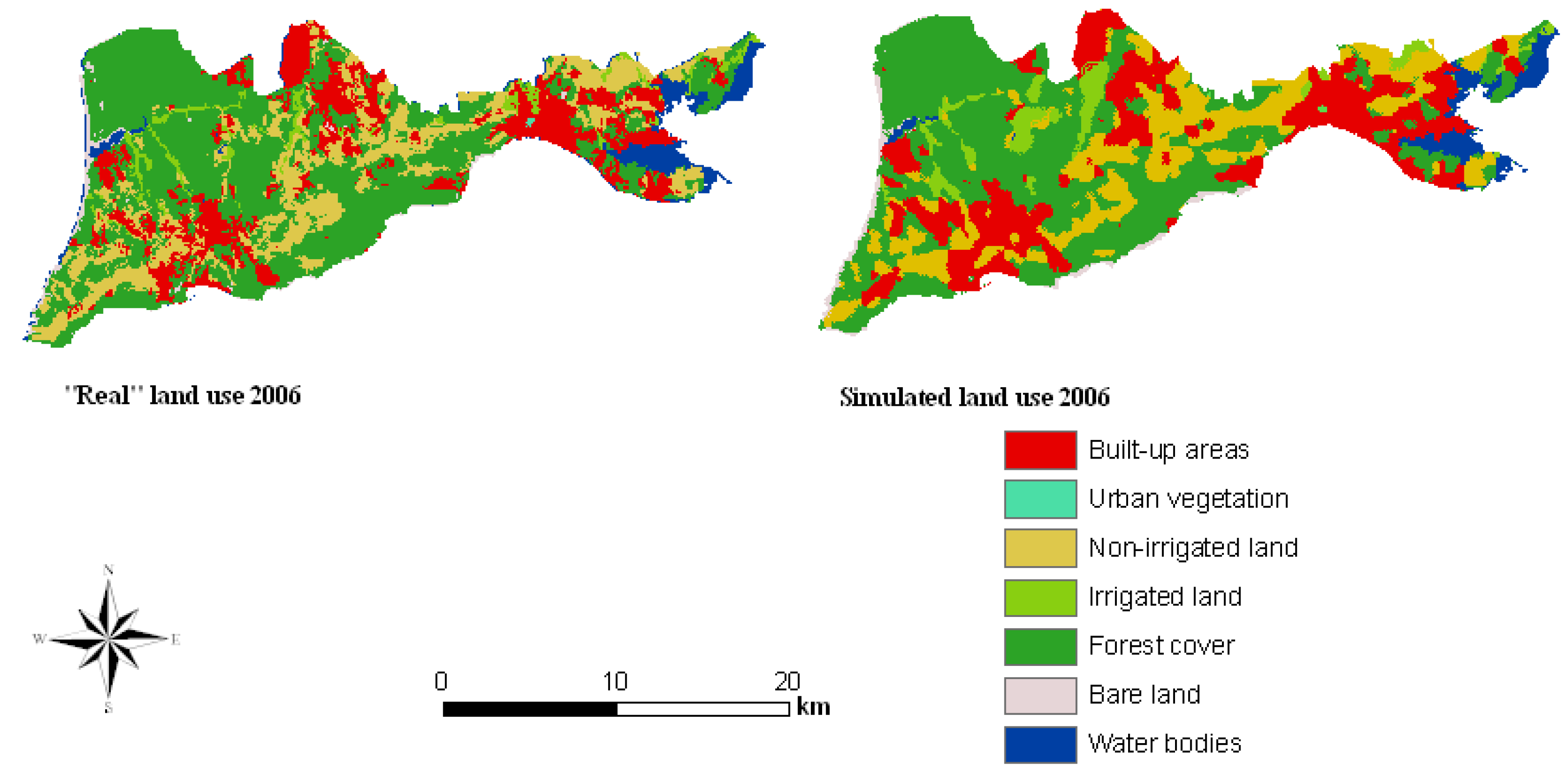
Visual interpretation of the modeling results (
Figure 4) shows that the simulated map for the year 2006 is reasonably similar to the “real” map for that year. A more detailed analysis was accomplished using the Kappa variations. The closer the values of these indices are to 100%, the stronger the agreement is between two maps. The
Kno, which also gives the overall accuracy of simulation [
31], is calculated to be 83%. The model performed very well in the ability to specify location correctly (
Klocation = 87%), and also in the ability to specify quantity (
Kquantity = 83%). However, it is important to note that some discrepancies are evident between the “real” and simulated land cover maps of 2006. This could be due to reasons such as inadequate suitability maps for modeling the phenomenon, generalizations applied for image classification results, and the shape of the contiguity filter used. The suitability maps have been used as rules during the modeling process and have had a great influence on the result. Results are also sensitive to the constraints and factors employed to define the rules.
Figure 4.
‘Actual’ and simulated land cover map for the year 2006.
Figure 4.
‘Actual’ and simulated land cover map for the year 2006.
After defining the parameters used for the calibration and modeling and assessing the validity, it was interesting to examine the pattern and tendency of change in a long-term simulation. Therefore, land cover projection for the year 2020 was performed in the same way (
Figure 5). A cross-tabulation that describes the changes in land cover classes included in the study is given in
Table 7. CA-Markov has the ability to simulate transition among any number of classes and the nature of the simulation is bidirectional. The table shown below demonstrates the number of pixels that are expected to change from 2006 to 2020. Two classes (bare land and water bodies) are not included in the matrix because the model did not predict any changes for 2020. The diagonal of the matrix indicates the number of pixels that have persisted during the simulation, while the off-diagonal shows the number pixels that changed class.
Figure 5.
Simulated land cover maps for the year 2020.
Figure 5.
Simulated land cover maps for the year 2020.
Table 7.
Cross-tabulation of actual land cover in 2006 with simulated land cover for 2020 (number of pixels).
Table 7.
Cross-tabulation of actual land cover in 2006 with simulated land cover for 2020 (number of pixels).
| | | Actual land cover map of 2006 |
|---|
| | Classes | Built-up areas | Urban veg. | Non-irrig. | Irrigated land | Forest cover | Total |
|---|
| Simulated land cover map of 2020 | Built-up areas | 9,777 | 2,276 | 86 | 3,178 | 391 | 15,708 |
| Urban veg. | 1,361 | 7,507 | 38 | 3,856 | 163 | 12,925 |
| Non-irrig. | 28 | 11 | 601 | 440 | 5 | 1,085 |
| Irrigated land | 1,079 | 3,035 | 310 | 23,775 | 426 | 28,625 |
| Forest cover | 248 | 628 | 11 | 1,310 | 1,070 | 3,267 |
| Bare land | 106 | 20 | 23 | 222 | 95 | 466 |
| Water bodies | 6 | 0 | 0 | 0 | 0 | 6 |
| Total | 12,605 | 13,477 | 1,069 | 32,781 | 2,150 | 62,082 |
6. Conclusions
The study area is situated in the productive alluvial plains and attractive coastal areas of the country. Consequently, the area experienced extensive conversion to urban land cover in the last few decades. This study assessed and modeled the trend of urban land cover changes in the area using an integrated approach including GIS, RS, and modeling tools.
LULC maps of the study area for the years 2000 and 2006 were obtained using an object-oriented approach and the derived maps provided new information on spatio-temporal distributions of built-up areas in the region. Results obtained from classification were validated and employed for further change analysis and modeling.
A critical analysis of the nature of urban land cover change was addressed and quantified using landscape metrics and urban sprawl measurements. Each of the metrics provided information on the nature of each index for the study site. The sprawl measurement, with the Shannon Entropy index, supports the claim that there has been a high rate of sprawl and dispersion of urban development in the studied period, causing a significant impact on the urban fringe. The driving forces behind the sprawl could be many, but one of the major factors was population growth, particularly in the period after 1970, with the end of Portuguese overseas colonies.
The spatial simulation technique employed produced satisfactory results that were confirmed by various Kappa summaries. This allowed us to project land change until the year 2020. Results indicate that urban growth might continue to expand further in the future, and might have an undeniable impact on land resources, unless some preservation mechanism is enacted. Future projections presented a satisfactory output for short term forecasting. However, it is important to caution that the approach applied in this study may not be the best approach for long-term simulation. CA-Markov analysis does not only consider a change from non-built to built-up areas, but also any kind of transition among any of the feature classes included in the analyses. A change from built-up areas to non-built-up areas is less likely in rapidly growing urban areas, but the simulation model applied does consider this possibility. Future work will consider all these limitations and apply an advanced modeling approach that would allow for long-term simulation.


