5.1. Time-Series of Spatially Averaged Datasets
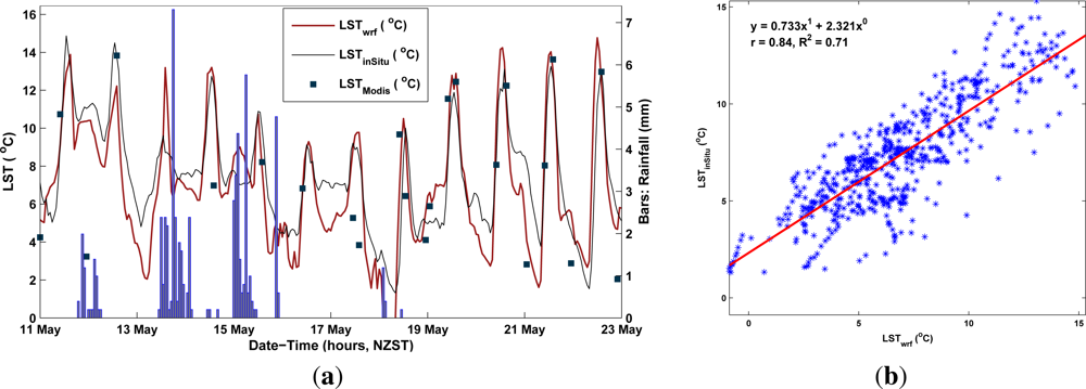
In this section, the results from the correlation analysis between the spatially averaged time-series of the three datasets are presented. First, we compared spatially averaged high resolution time-series of the WRF simulations with the
in situ measurements. Available MODIS LST observations were also overlaid on the
in situ and WRF series (
Figure 7(a)). This showed that the WRF and
in situ datasets have captured diurnal temperature cycle very closely over the measurement period. On the other hand, MODIS LST series have shown larger bias from both WRF and
in situ series. Hourly rainfall data from the UC Cass climate station was also analysed (
Figure 7(a)). LST
wrf and LST
inSitu 30-minute data showed a relatively strong (R
2 = 0.71) correlation (
Figure 7(b)). Afterwards, time-series of the WRF and the
in situ measurements were filtered according to the available MODIS LST observations. The filtered time-series of the
in situ data showed highest mean (
μ = 8.49) and lowest standard deviation (
σ = 3.26), while the MODIS LST time-series showed the lowest mean and the highest standard deviation (
Table 3). Comparison of the averaged time-series from the three datasets (which were filtered based on the available MODIS LST observations) revealed the differences in the LST at different dates (
Figure 8). While model simulations generally follow the
in situ dataset, the MODIS LST showed some significantly different observations from the
in situ measurements (such as points 3 and 8 in
Figure 8). There were a total of 25 coincident measurements over the study period, with 10 measurements over night and 15 measurements during day. During nighttime, 80% of the MODIS observations are lower compared with the
in situ measurements. During daytime, 73% of the MODIS temperatures are similar or higher and only in 23% of the cases lower than the
in situ data. This indicates that the lower mean LST from the MODIS time-series (
Table 3) is mainly due to night-time observations. Correlation with the
in situ time-series with no time-lag yields R
2 = 0.35 for the MODIS LST and R
2 = 0.77 for the WRF simulations (
Table 4(a)).
Time-lags were considered to account for the delay in warming and cooling of the surface as measured by the iButtons 1–2 cm below the surface versus instantaneously observed by the satellite. Taking the MODIS acquisition time as reference, lags of ±100 minute were applied on the
in situ data iteratively with 1 minute intervals and the regression R
2 values were calculated for each lag. For the correlation of model simulations with the
in situ data, lags were applied only to the
in situ measurements. Statistics from 0, 30, 60 and 90 minutes time-lags are given in the results (
Table 4).
Considering time-lags, correlations were generally deteriorated with lags of more than 90 minutes. The best agreement between the WRF model simulations with the
in situ data were obtained at 30 minute time-lag while the MODIS LST did so at about 90 min time-lag (
Table 4(a)). The model simulations also showed the highest agreement with the MODIS LST after adding a 30 min time-lag (
Table 4(a)). It is noteworthy that the highest correlation between the MODIS LST and the
in situ data is lower than the smallest value achieved from correlating the model simulations with the
in situ data. Surprisingly, the MODIS LST at all times has correlated better with the model simulations than with the
in situ data.
Several tests were made to improve the correlation values between the MODIS LST and the
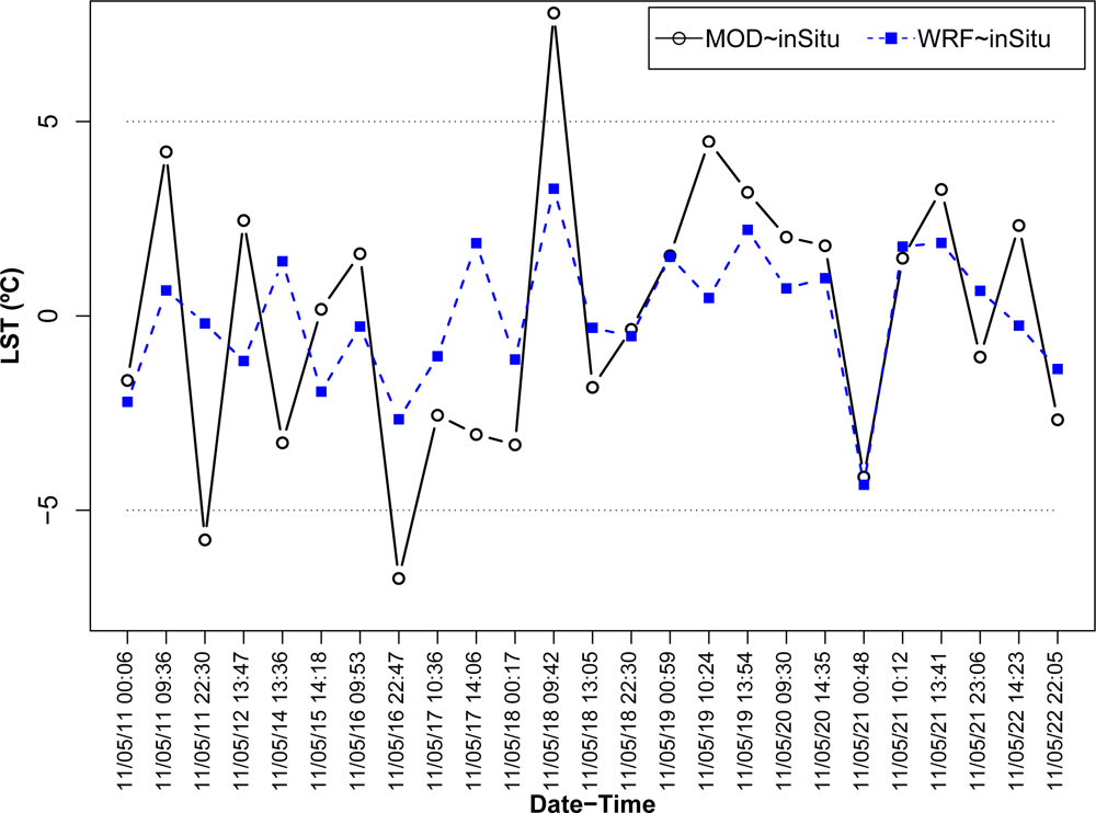
in situ data by detecting possible outliers based on the regression residuals and the scatter plots of the two datasets. Taking ±5 (≈ ±1.5
σ) as the upper and lower control limits for the regression residuals, three distinct outliers in the MODIS LST time-series appeared likely (
Figure 9). Since the residuals from the regression between LST
wrf and LST
inSitu were well inside the cut-off margins, it turned out that the source of the outliers to be in the MODIS LST dataset. The same outliers are also visible in the scatter plots (
Figure 10(a)). These points are lying farthest from the line-fit in the scatter plots of the two datasets (points bordered by a larger square in
Figure 10). The first two outliers from MODIS nighttime observations were considerably colder than the measured and modelled data. The third outlier was a MODIS morning observation, which was warmer than the temperatures in the other two datasets.
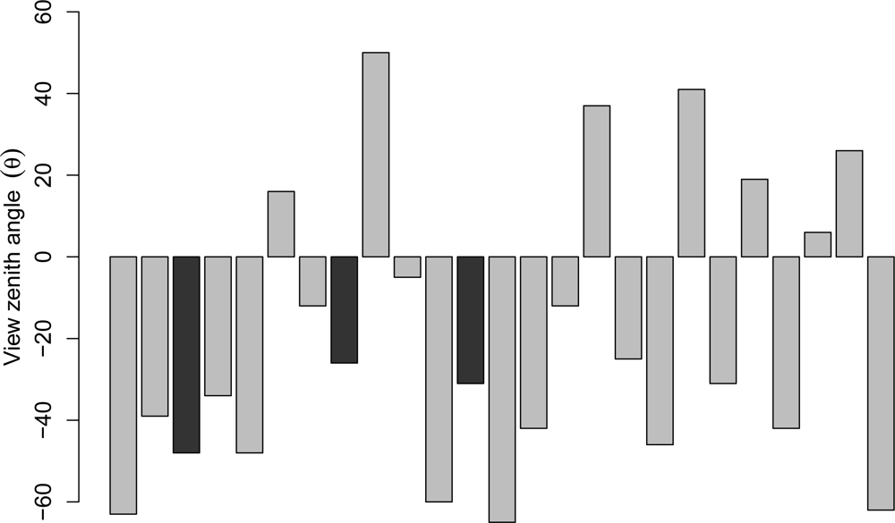
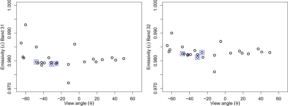
According to the overpass times (
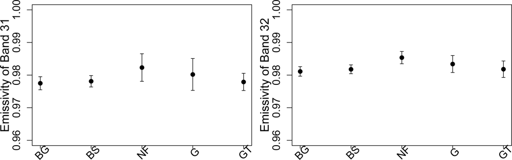
Figure 9), all outliers originate from the MODIS-Terra observations, and have appeared in the first half of the field experiment period. Because the view zenith angles of the outliers (48°, 26° and 31° from the East) are close or within the acceptable range of less than 45° [
2], it seems unlikely that the differences are due to unfavourable imaging geometry. Emissivity values of the outliers in both bands 31 & 32 are also within the standard range (
Figure 6).
We looked at relative humidity (RH) and other parameters from the model, but we did not find any meaningful pattern to explain the reason for the outliers. Since high amounts of atmospheric water vapour limits the accuracy of LST retrievals [
33] and, therefore, can be a reason for the outliers, we checked MODIS Total Precipitable Water or Water Vapor (MOD05, level 2, V5.1) product. Both near-infrared (1 km pixel-size, day only) and infrared (5 km pixel-size, day and night) fields were checked, however, there was no data over the study area for those dates when the outliers have occurred. We also checked the outliers against T
a data from the UC Cass climate station. This station is close to our test-site (3 km to the South) and is approximately at a similar elevation (583 m a.s.l.). In all three cases where the MODIS LST shows an outlier, T
a data were closer to the WRF simulations and the iButton measurements. For example, at point 8 (2011/05/16 22:47 in
Figure 8) the MODIS LST showed −1 °C, while T
a from the UC Cass weather station was 9.3 °C (average daily T
a was 7.9 °C). Also, soil temperature at 10 cm depth recorded in that station was 7.4 °C. These records are much closer to those from the WRF simulations and the
in situ measurements than to the MODIS LST (
Figure 8), which affirms the outliers in the latter dataset.
To prevent swamping and masking effects (see [
49]), outliers were removed sequentially, followed by the calculation of the new R
2 coefficient. Removing the largest outlier (obs. 12 in
Figure 9) improves R
2 from 0.35 to 0.51, removing the second largest outlier (point 8) improves R
2 to 0.53, and removing the third outlier (point 3) improves R
2 to 0.62 (
Figure 10(e)). With all the outliers removed, regression statistics were re-calculated for all time-lags (
Table 5(b) and
Figure 10).
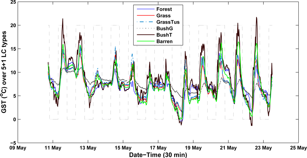
5.2. Land-Cover Based Time-series
Time-series of the MODIS LST and the model simulations over 5 LC classes were correlated individually versus the corresponding series of the
in situ data with and without time-lags (
Table 5). Time-lags with a range of ±100 minute, with 1 minute increments, were applied on the correlations between the MODIS LST and the
in situ series over all the LC types (
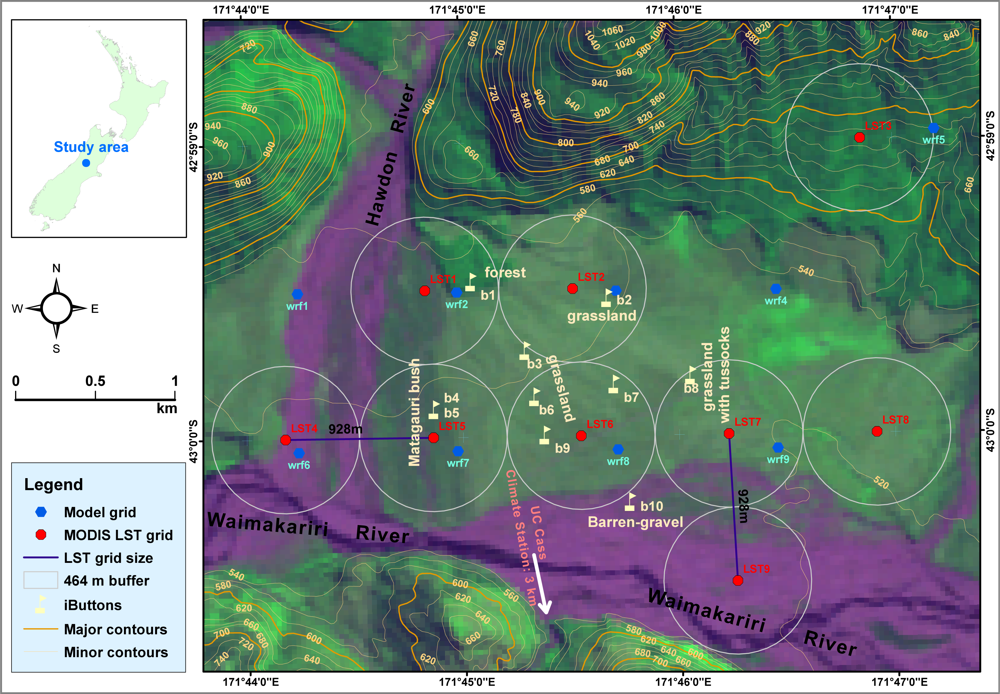
Figure 11). The five LC classes are Barren-Gravel (BG), Bush-Scrub (BS), Native-Forest (NF), Grassland (G) and Grass-Tussock (GT). For BG LC type there was no MODIS LST pixel overlapping the
in situ measurement points, therefore, a non-overlapping pixel with identical LC type has been used in the analysis. The MODIS LST pixel for the LC type NF suffered from high spectral mixing with only 25% fractional abundance (
Table 2). Another pixel with almost 100% forest cover (LST3), but higher elevation, was used in the spectral mixing of this point (
Figure 1).
Another point for consideration was the LC type BS. The height of the bush in the area is about 1 to 1.5 m from the base, with a moderate density of the scrub over the surface. Considering this point, the authors were concerned that the values of LST recorded by MODIS observation on this particular LC type are not exactly a representative of the skin temperature of the soil, but rather affected by the temperature near the top of the bush. Although the field experiment was conducted in mid-autumn, the bush maintained considerable foliage, which could have affected temperature measurements as well as solar radiation reaching the ground. Two iButtons were placed at this site, one on top of the bush (b5) and another one on the ground (b4). The corresponding data recorded at this site are referred to as “Bush-Scrub-Ground” (BSG) and “Bush-Scrub-Top” (BST). Correlation of these measurements with the corresponding MODIS LST pixel (LST5) showed higher agreement for BST compared with BSG (
Table 5). The strongest correlation from BST was observed at 19 min time-lag (R
2 = 0.77), with another peak at 60 min, then it dropped significantly when time-lag increased to 90 min (
Figure 11 and
Table 5). Also, for other LC classes correlations increased with time-lags between MODIS observations and the
in situ measurements. For LC type BG two pixels from LST
Modis were analysed: LST9 with homogeneous LC and LST4 with mixed LC. Both of them showed highest agreement with the
in situ data with ≈60 min time-lag; however, except for BST which is affected by the ambient T
a, LST4 showed the strongest correlation (R
2 = 0.68) than all LC types at all time-lags (
Table 5). The maximum improvements in the correlations between LST
wrf and LST
inSitu, as well as LST
Modis with LST
wrf were observed when ≈30 min time-lag was applied.
5.3. Comparison between Day and Night Measurements
In this section, the results from the regression analysis between the MODIS LST, the WRF model and the in situ data are presented by separating day and night observations. This analysis was necessary to discover the difference in time-lags at day/night and any possible anti-correlation due to differing surface temperature on each LC type at day or night.
Correlations between the MODIS LST and the
in situ data are generally stronger from the night series compared with those from the day series except for LC types GT and BG. LC type BS (“Bush-scrub”) showed more complex correlation pattern from day and night observations. During daytime, higher agreement is observed between the MODIS LST and the iButton measurements on top of the bush (BST in
Figure 12 with R
2 = 0.63) compared with the iButton on the ground (BSG in
Figure 12 with R
2 = 0.18), whereas during night a stronger correlation (R
2 = 0.94) is observed at the ground (BSG in
Figure 12). Barren-gravel LC type showed higher correlations over the pixel with higher mixing (LST4) both day and night. Although the other pixel in this LC class (LST9) had less mixing, correlations over that pixel are considerably lower (possible reasons can be shadowing effects of the mountain and contribution of the river water).
On the contrary, the WRF model simulations showed generally higher correlations with the
in situ data during day compared to night. Time-lags did not improve correlations between the WRF and the
in situ day-series (except for few cases with 30 min time-lag), however, some improvements were visible for time-lags of up to 60 min with night-series (
Figure 12).


