4.1. Measured Vegetation Characteristics for Different Habitat Categories
Our field survey found that
loggerhead shrikes prefer tall shrubs, especially thorny buffalo berry (
Sheperdia argentea) for nest locations, because thorny species most likely discourage mammalian predators. This is consistent with the results in a previous study by [
2]. Data analysis for the overstory showed that thorny buffalo berry occupies around 88% of tall shrubs in active sites, 91% in inactive sites, and 77% in control sites (
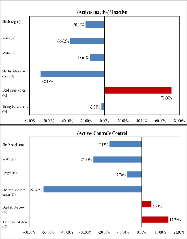
Table 1). The mean height of tall shrubs in active sites is 2.66 m, 20.12% shorter than that in inactive sites and 17.13% shorter than that in control sites (
Figure 8). The ANOVA outcomes identified a significant difference in mean height existing between active and inactive sites with a P-value 0.06, indicating that shrikes may have a preference in tall shrubs with a height lower than 3 m for nesting. In addition, the active sites have the highest canopy cover of dead shrubs with 34.4% among the three habitat categories, 42% greater than that in inactive sties and 5% greater than in control sites (
Figure 8). Therefore, shrike nesting sites are characterized by a high amount of dead materials, which was also supported by the significant difference between active and inactive sites in dead shrubs cover due to a P-value of 0.08 derived from ANOVA results. This is reasonable because shrikes can use dead branches to perch on while hunting for prey. Our analysis also revealed that dense thorny shrubs with less dead canopy in inactive sites are biophysical characteristics that may cause the site abandonment.
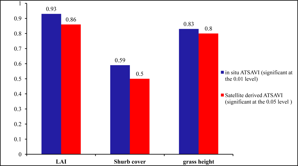
In the understory, active sites had the lowest LAI in comparison with the inactive and control sites. LAI has great potential in identifying nesting locations from non-nesting locations owing to the significant difference among the three habitat categories shown by the P values 0.01, 0.09, and 0.08. Therefore, the low LAI as well as less green biomass in active sites can strengthen the possibility that shrikes prefer nest locations with less grass productivity and more open spaces for easily identifying prey (
Figure 9). Similar results can be also found in previous studies by [
2,
27–
29] which concluded that shrikes prefer open habitats characterized by vegetation of lower stature. In addition, the averaged grass height in active sites was 0.31 m; significantly shorter than that in other habitat types, which is consistent with the findings in the study by [
30].
4.2. Measured Topographical Characteristics of Different Habitat Categories
Comparison of the topological characteristics among the three categories showed that shrikes’ occupied territories are farthest away from the roads at a higher elevation (
Table 4). On average, active sites, inactive sites, and control sites were 2,227 m, 1,779 m and 1,315 m away from the road respectively. This indicated that shrikes prefer to locate their nests further from the roads to avoid jeopardizing the roadside habitats in predation, which is in accordance with the explanations by [
29,
31]. We also found that the elevation for active sites and for control sites is significantly different (P < 0.1). The active sites were, on average, at an elevation 4 m higher than inactive sites, and 6 m higher than control sites, possibly indicating that the high elevation of active sites can reduce predation rates and provide more food availability for shrikes in comparison with the other two sites.
4.6. Suitable Shrike Habitat Modeling
The logistic regression coefficient, its standard error, and Wald test were shown in
Table 7. The ratio of regression coefficient to standard error, squared, equals the Wald statistic. If the Wald statistic is significant (
i.e., less than 0.05) then the parameter is useful to the model. For example, we can see that dead shrub canopy cover, shrub patch width, shrub patch height in
Table 7(D, G, and H) resulted in a small Wald statistic, therefore, and these three variables might be useful to build the regression models.
The log likelihood, Pseudo R
2 (Cox & Snell R
2 and Nagelkerke R
2), overall predicted correct, and Hosmer & Lemeshow test were presented in
Table 7 to evaluate the models. R
2 is comparable to R
2 from ANOVA conducted on individual observations. The interpretation of the log likelihood and Pseudo R
2 is: the less log likelihood, the higher R
2, the more proportion of variation in the dependent variable accounted for by the independent variable or variables. In this case, 21% of variation in active or inactive of habitat sites was accounted for by an index of the dead shrub canopy cover. Comparing
Table 7(D, G) we saw that the model with ‘dead shrub canopy cover’ accounted for 1% less of the variation in active and inactive than did the model with ‘shrub patches width’: the latter variable had a less log likelihood and, consequently, a greater Psuedo R
2. Hosmer & Lemeshow Test is a goodness-of-fit test of the null hypothesis that the model adequately fits the data. If the null is true, the statistic should have an approximately chi-square distribution with the displayed degrees of freedom. If the significance of the test is small (
i.e., less than 0.05) then the model does not adequately fit the data.
Table 7(D) showed a close chi-square distribution (7.71) with the displayed degrees of freedom (7) and the significance (0.36) was greater than 0.05, then the model should fit the data. The overall predicted correct helped to assess the performance of the models.
Having obtained the results in
Table 7(A–M), we conducted a multiple logistic regression analysis to determine how many different factors may be contributing to variation in the active habitat presence. We therefore ran another model, with the stepwise method to select the suitable independent variables, shown in
Table 7(N). In this case, we saw that only two variables, ATSAVI and ‘Shrub dead canopy cover’, were selected to enter the model. The effect of each of the 2 variables was significant when controlling for the effect of the other. Note that the Pseudo R
2 for the 2-variable model was higher compared to the Pseudo R
2 for all other single variable models in
Table 7(A–M). Thus, by including both ATSAVI and ‘Shrub dead canopy cover’ in the model, we are able to increase the Pseudo R
2. We also examined the goodness of fit of the model in
Table 7N and the results showed that no reason to reject the fit of the model, implying that the assumption made in logistic regression that residuals are binomially distributed was satisfied. The higher predicted correct in
Table 7(N) (72%) showed the predicted probability of the model for nesting presence. Based on
Table 7(N), the logistic model for suitable habitat mapping should be:
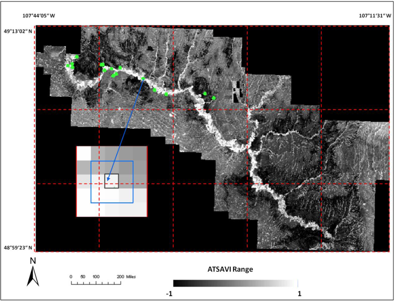
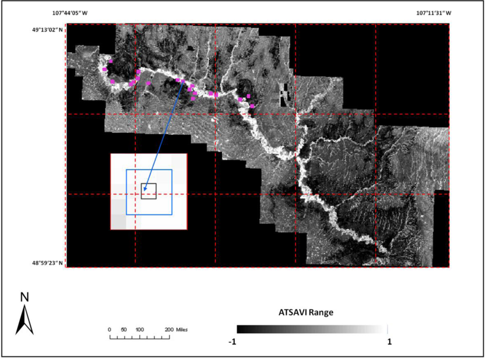
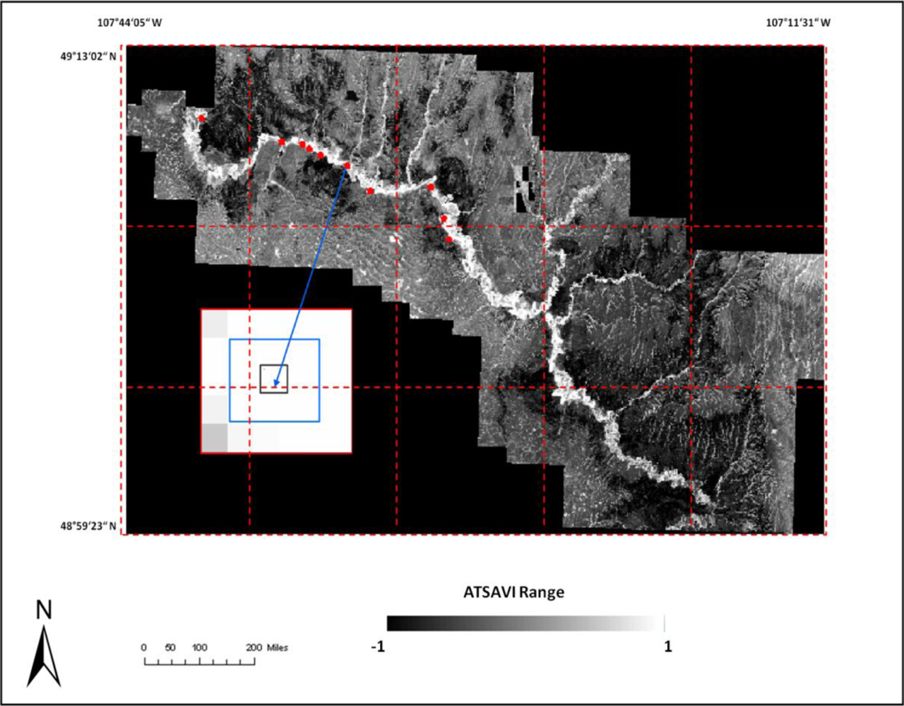
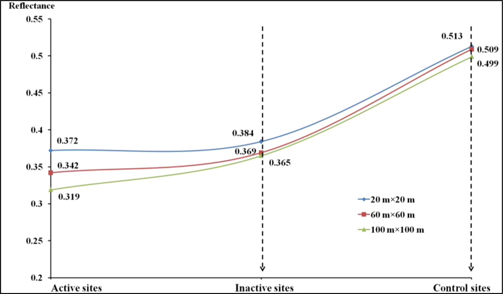
where Ds is dead material in tall shrub canopy. From above equation we can see that dead material in tall shrub canopy positive contribute to the shrike nest selection, and ATSAVI negatively contributes to the shrike nest selection. The ATSAVI is a greater negative contributor. This conclusion is consistent with the ATSAVI variation for different shrike habitat types which is shown in
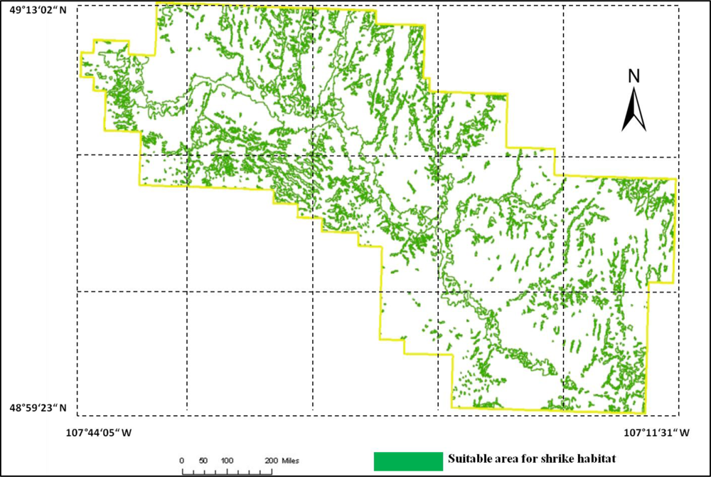
Figure 11. This model was applied to the SPOT image to derive the suitable habitat map for
loggerhead shrike in GNPC (
Figure 13). This map is a polygon file and can be easily used by Parks manager.
4.7. Uncertainties and Opportunities
As a preliminary research, our research suffers from several limitations and uncertainties. First, this study relied on Andrew Didiuk (Environment Canada, Canadian Wildlife Service) survey of loggerhead shrike nests in 2004 for baseline locations. Some shrike nests in GNPC might have not been accurately known, and the outliner or absence of records may result in inadequate exploration of shrike habitats. It is necessary to resurvey the study area in order to obtain more reliable sample data. Because the uncertainty arising from insufficient field datasets can lead to difficulty in validating the accuracy of habitat estimation. Other limiting factors include climate variation (temperature and precipitation), grazing, burning, and surrounding land-use activities (land conversions) that all might affect shrike abundance [
33–
35].
Uncertainties can also be found in the field survey which covers quite a large area. In such situation, a gradient analysis method should have more potential than non-gradient approaches for accurately investigating habitat characteristics along the environmental gradient. Possible gradient methods contain PCA (principle component analysis), CA (Correspondence analysis), or DCA (detrended correspondence analysis). This can be promising a direction for our further research to improve the results.
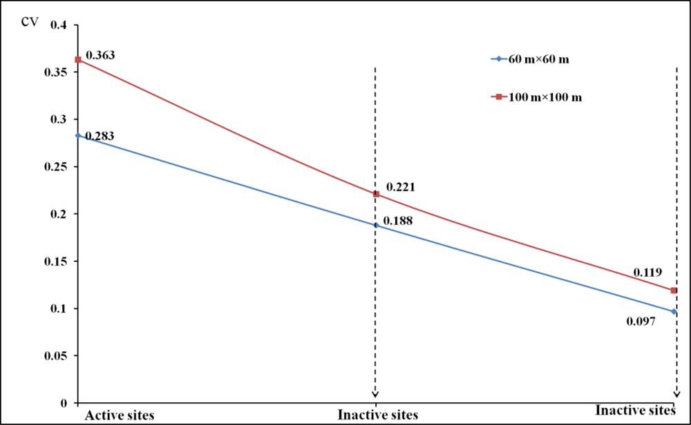
For remote sensing perspective of spatial heterogeneity, CV (Coefficient of variance) analysis can be further validated by measures such as landscape indices, fragmentation/connectivity measure, image segmentation, or image texture (e.g., GLCM-grey level co-occurrence matrix). However, due to the low spatial resolution of our available satellite imagery and the high level of heterogeneity of our study area, currently landscape indices and image segmentation performed poorly in this study for extracting meaningful information from shrike habitats.
Therefore, in order to eliminate or minimize the aforementioned uncertainties in our study, three important concerns need to be addressed in future research: (1) applying comprehensive census methods to detect more shrike nests in the study area; (2) investigating multiple habitat impacting factors.
