Trend Change Detection in NDVI Time Series: Effects of Inter-Annual Variability and Methodology

 , and
, and
Abstract
:
1. Introduction
2. Data and Methods
2.1. GIMMS NDVI3g Dataset
2.2. Breakpoint Detection Algorithm
2.3. Methods for Trend Estimation
2.3.1. Trend Estimation on Annual Aggregated Time Series (Method AAT)
2.3.2. Trend Estimation Based on a Season-Trend Model (Method STM)
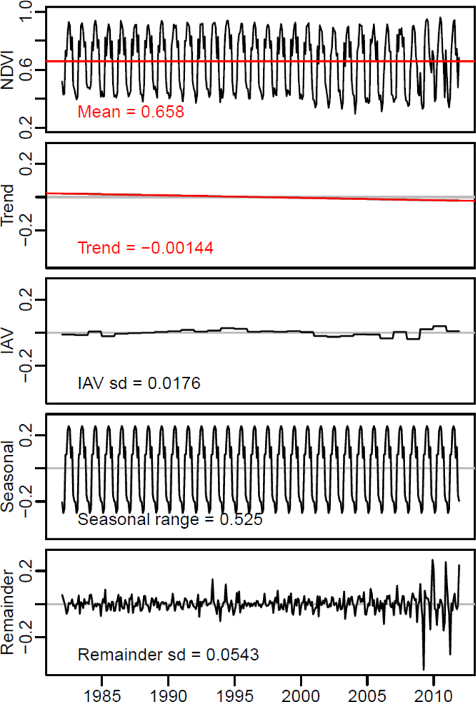
2.3.3. Trend Estimation on De-Seasonalized Time Series
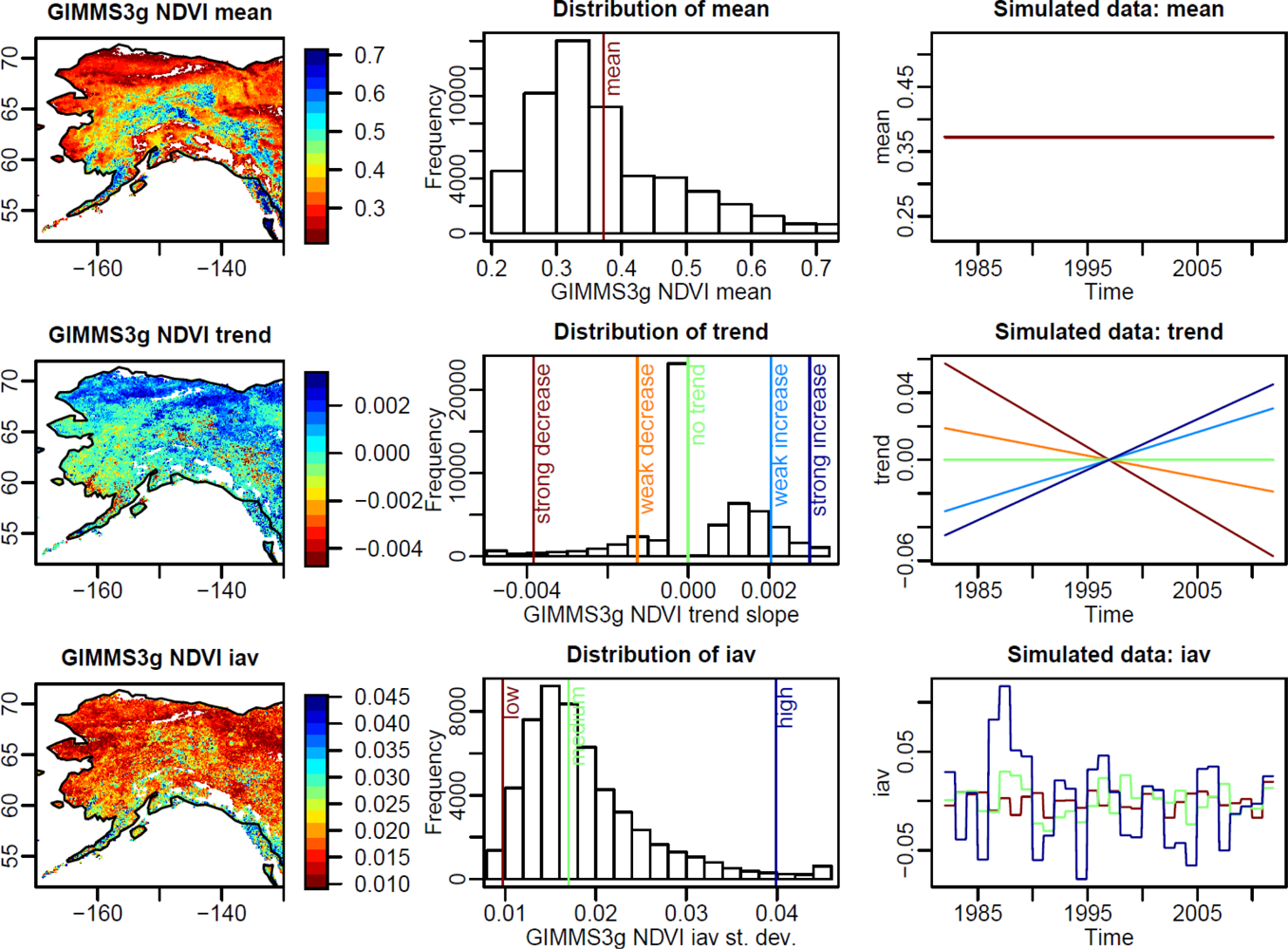
2.4. Simulation of Surrogate Time Series
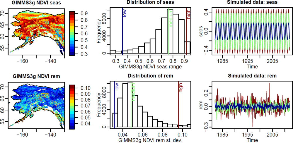
2.4.1. Estimation of Inter-Annual Variability, Seasonality and Short-Term Variability from Observed Time Series
- (1)
- The mean of each NDVI time series was calculated.
- (2)
- In the second step, monthly values were averaged to annual values and the trend was calculated according to method AAT but without computing breakpoints. Hence, the slope of the annual NDVI trend over the full length of the time series was estimated.
- (3)
- To estimate the inter-annual variability, the standard deviation and range of the annual anomalies were calculated. The mean of the time series and the derived trend component from step (2), were subtracted from the annual values to derive the trend-removed and mean-centred annual values (annual anomalies). If the trend slope was not significant (p > 0.05), only the mean was subtracted. The standard deviation and the range of the annual anomalies were computed as measures for the inter-annual variability of the time series.
- (4)
- In the next step, the range of the seasonal cycle was estimated. The mean, the trend component and the annual anomalies were subtracted from the original time series to calculate a detrended, centered and for annual anomalies adjusted time series. Based on this time series the seasonal cycle was estimated as the mean seasonal cycle and the range was computed.
- (5)
- In the last step, the standard deviation and the range of the short-term anomalies were computed. Short-term anomalies were computed by subtracting the mean, the trend component, the annual anomalies and the mean seasonal cycle from the original time series. The result is the remainder time series component. The standard deviation of the remainder time series component is a measure of short-term variability.
2.4.2. Surrogate Time Series and Factorial Experiment
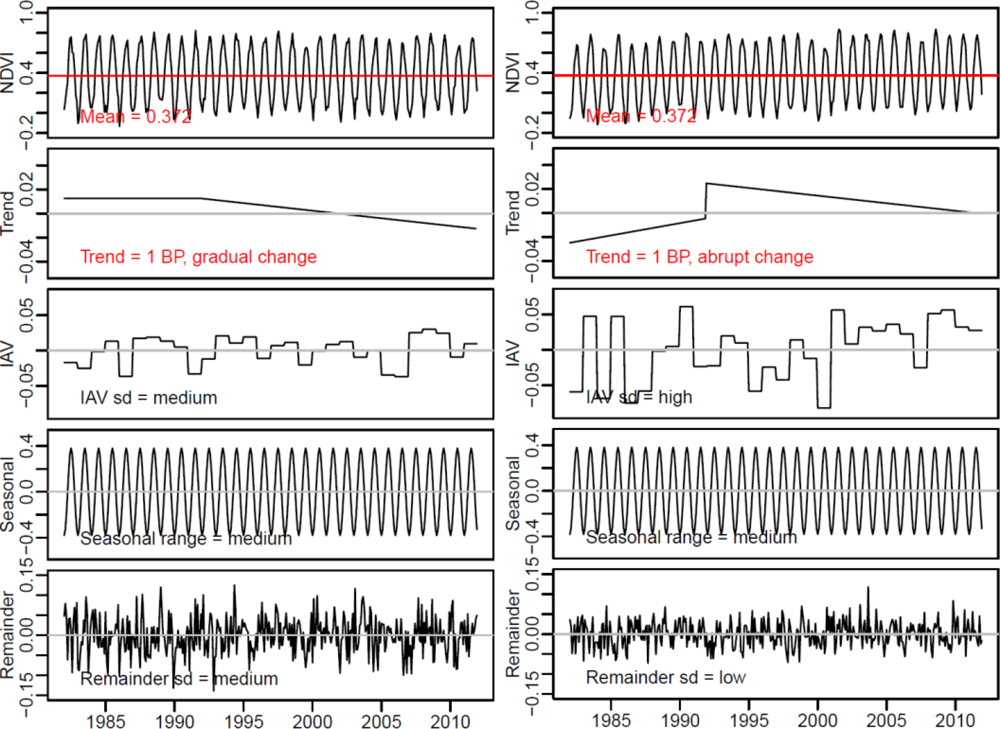
- (1)
- Trend: Time series with strong and weak positive, strong and weak negative and without a trend were created. Different magnitudes of trend slopes were derived from the 1% percentile of the observed distribution of trend slopes (strong decrease), 25% percentile (weak decrease), median (no trend), 75% percentile (weak increase) and 99% percentile (strong increase), respectively.
- (2)
- Inter-annual variability: Time series with low, medium and high inter-annual variability were created based on normal-distributed random values with zero mean and a standard deviation according to the 1%, 50% and 99% percentiles of the observed distribution of the standard deviation of annual anomalies. Values outside the observed ranges of inter-annual variability were set to the minimum or maximum of the observed distribution, respectively.
- (3)
- Seasonality: Seasonal cycles based on a harmonic model with low, medium, and high amplitudes were created according to the observed 1%, 50% and 99% percentiles of the distribution of seasonal ranges.
- (4)
- Short-term variability: Different levels of short-term variability were created based on normal-distributed random values with zero mean and a standard deviation according to the 1%, 50% and 99% percentiles of the observed distribution of the standard deviation of remainder time series values.
- (1)
- Type of trend and number of breakpoints/segments (maximum 2 breakpoints = maximum 3 segments per time series with positive, negative or no trend = 27 possibilities),
- (2)
- Trend magnitude (weak, strong),
- (3)
- Inter-annual variability (low, medium, high),
- (4)
- Short-term variability (low, medium, high),
- (5)
- Type of trend change (gradual, abrupt) and
- (6)
- Range of seasonal cycle (low, medium, high).
2.5. Evaluation of Method Performances
2.5.1. Evaluation of Breakpoints
2.5.2. Evaluation of Trend Slopes and Significances
- N3: significant negative trend (slope < 0 and p ≤ 0.05)
- N2: non-significant negative trend (slope < 0 and 0.05 < p ≤ 0.1)
- N1: no trend with negative tendency (slope < 0 and p > 0.1)
- P1: no trend with positive tendency (slope > 0 and p > 0.1)
- P2: non-significant positive trend (slope > 0 and 0.05 < p ≤ 0.1)
- P3: significant positive trend (slope > 0 and p ≤ 0.05).
2.5.3. Evaluation of the Overall Performance for Trend and Breakpoint Estimation
2.6. Application to Real Time Series of Alaska: Ensemble of NDVI Trends
3. Results
3.1. Observed and Simulated Properties of NDVI Time Series
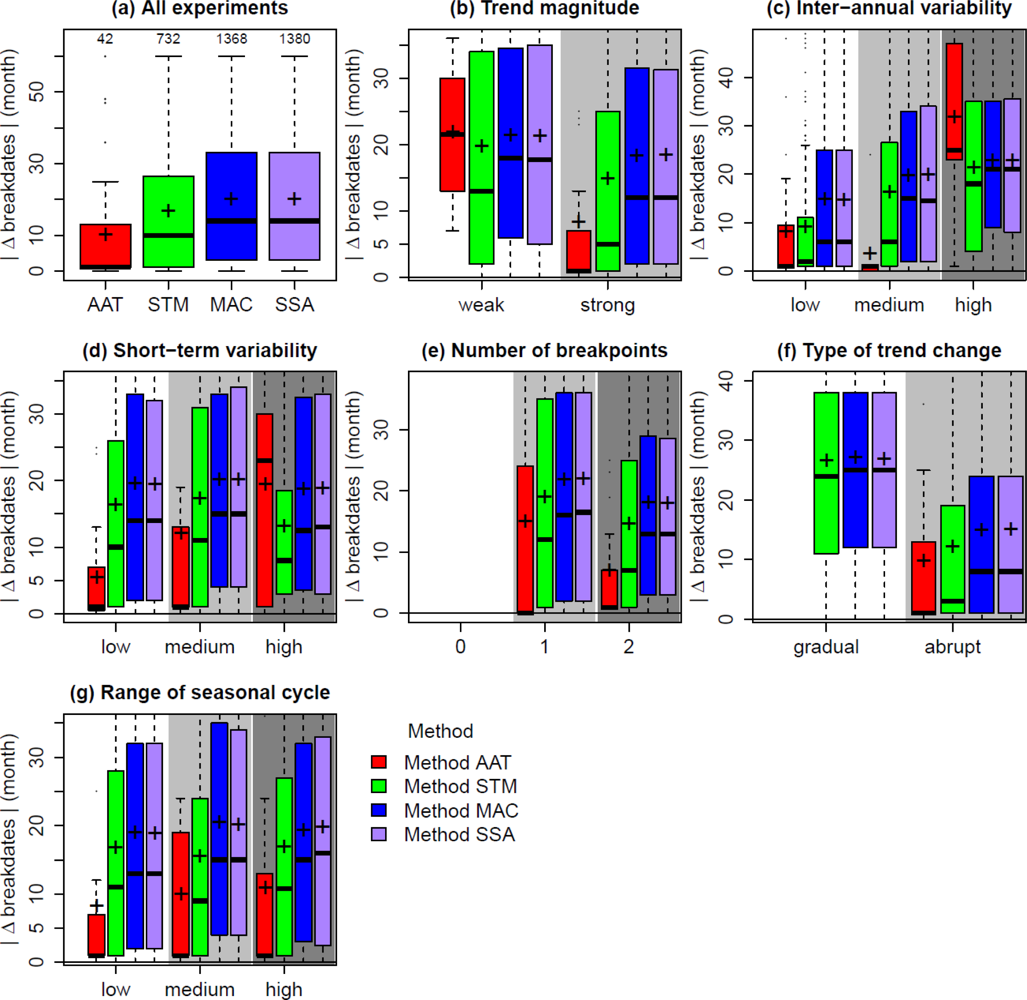
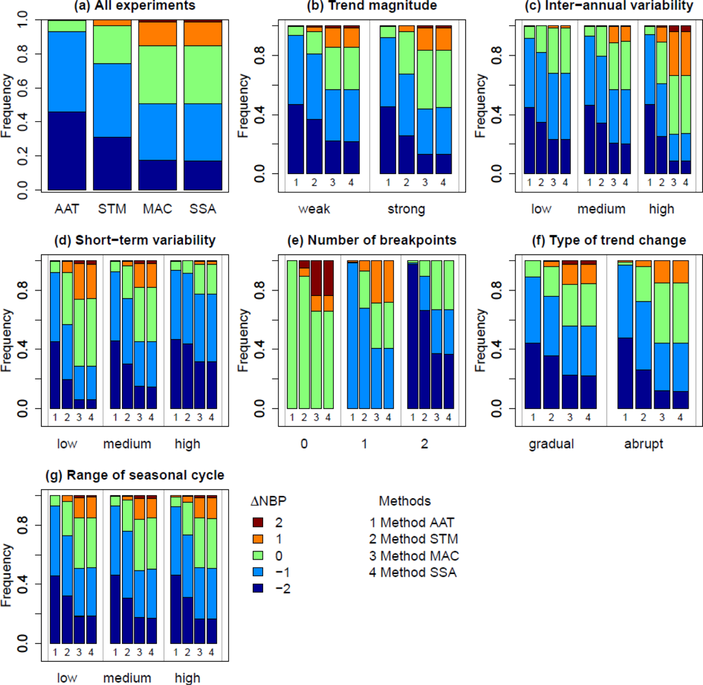
3.2. Evaluation of Estimated Breakpoints
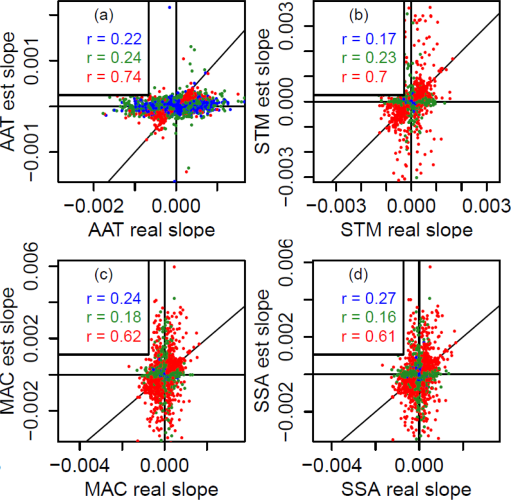
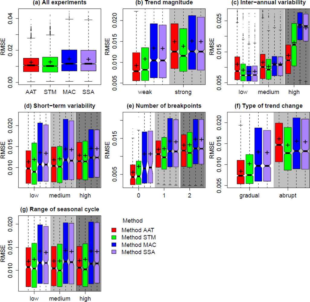
3.3. Evaluation of Estimated Trends
3.4. Effects on the Overall Performance of the Methods
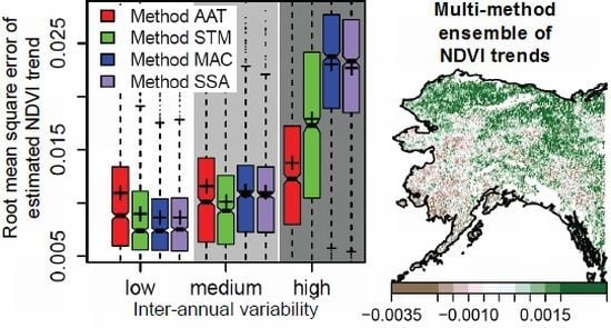
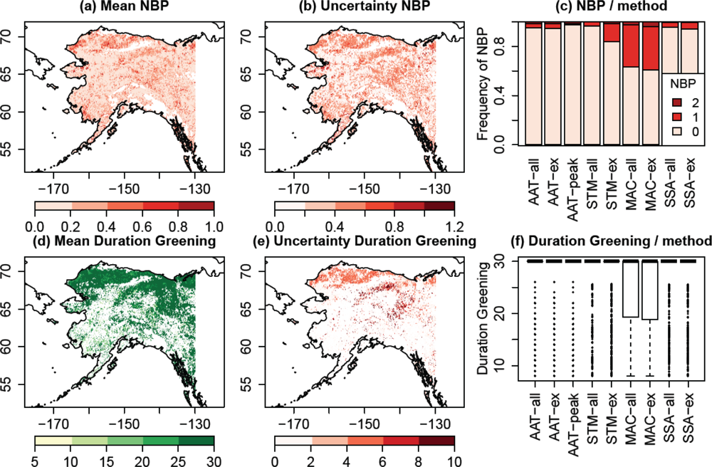
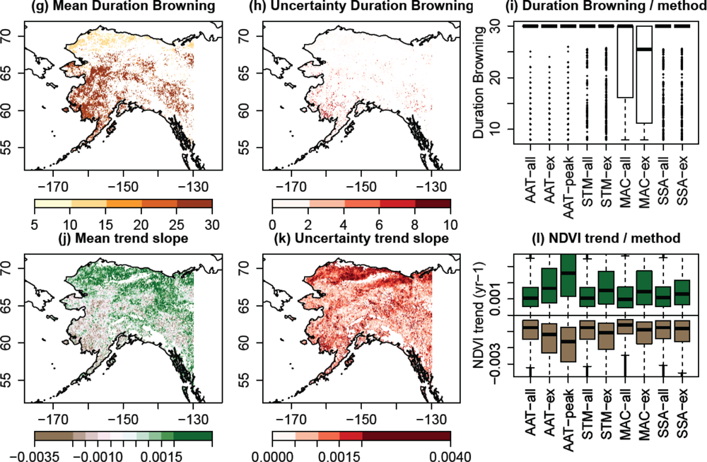
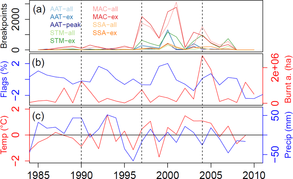
3.5. Multi-Method Ensemble of Breakpoint and Trend Estimates in Alaska
4. Discussion
4.1. Effect of Temporal Resolution on Method Performance
4.2. Effect of Trend Changes on Method Performance
4.3. Effect of Inter-Annual Variability on Method Performance
4.4. Plausibility of Trend and Breakpoint Estimates in Alaska
4.5. Practical Recommendations
5. Conclusions
Acknowledgments
- Conflict of InterestThe authors declare no conflict of interest.
References and Notes
- Lucht, W.; Schaphoff, S.; Erbrecht, T.; Heyder, U.; Cramer, W. Terrestrial vegetation redistribution and carbon balance under climate change. Carbon Balance Manage. 2006, 1, 6. [Google Scholar]
- Coppin, P.; Jonckheere, I.; Nackaerts, K.; Muys, B.; Lambin, E. Digital change detection methods in ecosystem monitoring: A review. Int. J. Remote Sens. 2004, 25, 1565–1596. [Google Scholar]
- Tucker, C.J. Red and photographic infrared linear combinations for monitoring vegetation. Remote Sens. Environ. 1979, 150, 127–150. [Google Scholar]
- Turner, D.P.; Cohen, W.B.; Kennedy, R.E.; Fassnacht, K.S.; Briggs, J.M. Relationships between leaf area index and Landsat TM spectral vegetation indices across three temperate zone sites. Remote Sens. Environ. 1999, 70, 52–68. [Google Scholar]
- Gamon, J.A.; Field, C.B.; Goulden, M.L.; Griffin, K.L.; Hartley, E.; Joel, G.; Peñuelas, J.; Valentini, R. Relationships between NDVI, canopy structure, and photosynthesis in three californian vegetation types. Ecol. Appl. 1995, 5, 28–41. [Google Scholar]
- Fensholt, R.; Sandholt, I.; Rasmussen, M.S. Evaluation of Modis LAI, FAPAR and the relation between FAPAR and NDVI in a semi-arid environment using in situ measurements. Remote Sens. Environ. 2004, 91, 490–507. [Google Scholar]
- Myneni, R.B.; Hall, F.G.; Sellers, P.J.; Marshak, A.L. The interpretation of spectral vegetation indexes. IEEE Trans. Geosci. Remote Sens. 1995, 33, 481–486. [Google Scholar]
- DeFries, R.; Hansen, M.; Townshend, J. Global discrimination of land cover types from metrics derived from AVHRR pathfinder data. Remote Sens. Environ. 1995, 54, 209–222. [Google Scholar]
- Tucker, C.J.; Slayback, D.A.; Pinzon, J.E.; Los, S.O.; Myneni, R.B.; Taylor, M.G. Higher northern latitude normalized difference vegetation index and growing season trends from 1982 to 1999. Int. J. Biometeorol. 2001, 45, 184–190. [Google Scholar]
- Myneni, R.B.; Keeling, C.D.; Tucker, C.J.; Asrar, G.; Nemani, R.R. Increased plant growth in the northern high latitudes from 1981 to 1991. Nature 1997, 386, 698–702. [Google Scholar]
- Lucht, W.; Prentice, I.C.; Myneni, R.B.; Sitch, S.; Friedlingstein, P.; Cramer, W.; Bousquet, P.; Buermann, W.; Smith, B. Climatic control of the high-latitude vegetation greening trend and pinatubo effect. Science 2002, 296, 1687–1689. [Google Scholar]
- Myers-Smith, I.H.; Forbes, B.C.; Wilmking, M.; Hallinger, M.; Lantz, T.; Blok, D.; Tape, K.D.; Macias-Fauria, M.; Sass-Klaassen, U.; Lévesque, E.; et al. Shrub expansion in tundra ecosystems: Dynamics, impacts and research priorities. Environ. Res. Lett. 2011, 6, 045509–045509. [Google Scholar]
- Goetz, S.J.; Bunn, A.G.; Fiske, G.J.; Houghton, R.A. Satellite-observed photosynthetic trends across boreal north america associated with climate and fire disturbance. Proc. Natl. Acad. Sci. USA 2005, 102, 13521–13525. [Google Scholar]
- Bunn, A.G.; Goetz, S.J.; Kimball, J.S.; Zhang, K. Northern high-latitude ecosystems respond to climate change. Eos Trans. AGU 2007, 88, 333–333. [Google Scholar]
- Wang, X.; Piao, S.; Ciais, P.; Li, J.; Friedlingstein, P.; Koven, C.; Chen, A. Spring temperature change and its implication in the change of vegetation growth in North America from 1982 to 2006. Proc. Natl. Acad. Sci. USA 2011, 108, 1240–1245. [Google Scholar]
- Piao, S.; Wang, X.; Ciais, P.; Zhu, B.; Wang, T.; Liu, J. Changes in satellite-derived vegetation growth trend in temperate and boreal Eurasia from 1982 to 2006. Glob. Change Biol. 2011, 17, 3228–3239. [Google Scholar]
- Beck, P.S.A.; Goetz, S.J. Satellite observations of high northern latitude vegetation productivity changes between 1982 and 2008: Ecological variability and regional differences. Environ. Res. Lett. 2011, 6, 45501–45501. [Google Scholar]
- Fensholt, R.; Proud, S.R. Evaluation of earth observation based global long term vegetation trends—Comparing GIMMS and MODIS global NDVI time series. Remote Sens. Environ. 2012, 119, 131–147. [Google Scholar]
- Tucker, C.; Pinzon, J.; Brown, M.; Slayback, D.; Pak, E.; Mahoney, R.; Vermote, E.; El Saleous, N. An extended AVHRR 8-km NDVI dataset compatible with MODIS and spot vegetation NDVI data. Int. J. Remote Sens. 2005, 26, 4485–4498. [Google Scholar]
- Alcaraz-Segura, D.; Chuvieco, E.; Epstein, H.E.; Kasischke, E.S.; Trishchenko, A. Debating the greening vs. Browning of the north american boreal forest: Differences between satellite datasets. Glob. Change Biol. 2010, 16, 760–770. [Google Scholar]
- Parent, M.B.; Verbyla, D. The browning of Alaska’s boreal forest. Remote Sens. 2010, 2, 2729–2747. [Google Scholar]
- Fraser, R.H.; Olthof, I.; Carrière, M.; Deschamps, A.; Pouliot, D. Detecting long-term changes to vegetation in northern Canada using the Landsat satellite image archive. Environ. Res. Lett. 2011, 6, 045502–045502. [Google Scholar]
- Beck, P.S.A.; Juday, G.P.; Alix, C.; Barber, V.A.; Winslow, S.E.; Sousa, E.E.; Heiser, P.; Herriges, J.D.; Goetz, S.J. Changes in forest productivity across Alaska consistent with biome shift. Ecol. Lett. 2011, 14, 373–379. [Google Scholar]
- Berner, L.T.; Beck, P.S.A.; Bunn, A.G.; Lloyd, A.H.; Goetz, S.J. High-latitude tree growth and satellite vegetation indices: Correlations and trends in Russia and Canada (1982–2008). J. Geophys. Res.-Biogeosci. 2011, 116. [Google Scholar] [CrossRef]
- Verbyla, D. Browning boreal forests of western north america. Environ. Res. Lett. 2011, 6, 41003–41003. [Google Scholar]
- Sulkava, M.; Luyssaert, S.; Rautio, P.; Janssens, I.A.; Hollmén, J. Modeling the effects of varying data quality on trend detection in environmental monitoring. Ecol. Inform. 2007, 2, 167–176. [Google Scholar]
- Eklundh, L.; Olsson, L. Vegetation index trends for the African Sahel 1982–1999. Geophys. Res. Lett. 2003, 30, 1–4. [Google Scholar]
- de Beurs, K.M.; Henebry, G.M. Trend analysis of the pathfinder AVHRR land (PAL) NDVI data for the deserts of central Asia. IEEE Geosci. Remote Sens. Lett. 2004, 1, 282–286. [Google Scholar]
- de Beurs, K.M.; Henebry, G.M. A land surface phenology assessment of the northern polar regions using MODIS reflectance time series. Can. J. Remote Sens. 2010, 36, S87–S110. [Google Scholar]
- Verbesselt, J.; Hyndman, R.; Newnham, G.; Culvenor, D. Detecting trend and seasonal changes in satellite image time series. Remote Sens. Environ. 2010, 114, 106–115. [Google Scholar]
- de Jong, R.; de Bruin, S.; de Wit, A.; Schaepman, M.E.; Dent, D.L. Analysis of monotonic greening and browning trends from global NDVI time-series. Remote Sens. Environ. 2011, 115, 692–702. [Google Scholar] [Green Version]
- Mahecha, M.D.; Fürst, L.M.; Gobron, N.; Lange, H. Identifying multiple spatiotemporal patterns: A refined view on terrestrial photosynthetic activity. Pattern Recogn. Lett. 2010, 31, 2309–2317. [Google Scholar]
- Verbesselt, J.; Hyndman, R.; Zeileis, A.; Culvenor, D. Phenological change detection while accounting for abrupt and gradual trends in satellite image time series. Remote Sens. Environ. 2010, 114, 2970–2980. [Google Scholar]
- Wu, Z.; Schneider, E.K.; Kirtman, B.P.; Sarachik, E.S.; Huang, N.E.; Tucker, C.J. The modulated annual cycle: An alternative reference frame for climate anomalies. Clim. Dyn. 2008, 31, 823–841. [Google Scholar]
- de Jong, R.; Verbesselt, J.; Schaepman, M.E.; Bruin, S. Trend changes in global greening and browning: Contribution of short-term trends to longer-term change. Glob. Change Biol. 2011, 18, 642–655. [Google Scholar]
- de Jong, R.; Verbesselt, J.; Zeileis, A.; Schaepman, M. Shifts in global vegetation activity trends. Remote Sens. 2013, 5, 1117–1133. [Google Scholar]
- Bai, J.; Perron, P. Computation and analysis of multiple structural change models. J. Appl. Econometr. 2003, 18, 1–22. [Google Scholar]
- Pinzon, J.; et al. Revisiting error, precision and uncertainty in ndvi avhrr data: Development of a consistent NDVI3g time series. Remote Sens. 2013. this volume.. [Google Scholar]
- Xu, L.; Myneni, R.B.; Chapin, F.S., III; Callaghan, T.V.; Pinzon, J.E.; Tucker, C.J.; Zhu, Z.; Bi, J.; Ciais, P.; Tommervik, H.; et al. Temperature and vegetation seasonality diminishment over northern lands. Nature Clim. Change 2013. [Google Scholar] [CrossRef]
- Kaufmann, R.K.; Zhou, L.; Knyazikhin, Y.; Shabanov, V.; Myneni, R.B.; Tucker, C.J. Effect of orbital drift and sensor changes on the time series of avhrr vegetation index data. IEEE Trans. Geosci. Remote Sens. 2000, 38, 2584–2597. [Google Scholar]
- Holben, B.N. Characteristics of maximum-value composite images from temporal AVHRR data. Int. J. Remote Sens. 1986, 7, 1417–1434. [Google Scholar]
- Zeileis, A.; Kleiber, C.; Krämer, W.; Hornik, K. Testing and dating of structural changes in practice. Computat. Statist. Data Anal. 2003, 44, 109–123. [Google Scholar]
- Mann, H.B. Nonparametric tests against trend. Econometrica 1945, 13, 245–259. [Google Scholar]
- Verbesselt, J.; Zeileis, A.; Herold, M. Near real-time disturbance detection using satellite image time series. Remote Sens. Environ. 2012, 123, 98–108. [Google Scholar]
- Golyandina, N.; Nekrutkin, V.V.; Zhigljavskiy, A.A. Analysis of Time Series Structure: SSA and Related Techniques; Chapman & Hall/CRC: Boca Raton, FL, USA, 2001; p. 305. [Google Scholar]
- Foody, G.M. Status of land cover classification accuracy assessment. Remote Sens. Environ. 2002, 80, 185–201. [Google Scholar]
- Congalton, R.G. A review of assessing the accuracy of classifications of remotely sensed data. Remote Sens. Environ. 1991, 37, 35–46. [Google Scholar]
- Deming, W.E.; Stephan, F.F. On a least squares adjustment of a sampled frequency table when the expected marginal totals are known. Ann. Math. Statist. 1940, 11, 427–444. [Google Scholar]
- Kasischke, E.S.; Williams, D.; Barry, D. Analysis of the patterns of large fires in the boreal forest region of Alaska. Int. J. Wildland Fire 2002, 11, 131–144. [Google Scholar]
- FRAMES: Alaska Large Fire Database. 2011.
- Schneider, U.; Fuchs, T.; Meyer-Christoffer, A.; Rudolf, B. Global Precipitation Analysis Products of the GPCC. http://www.dwd.de/bvbw/generator/DWDWWW/Content/Oeffentlichkeit/KU/KU4/KU42/en/Reports__Publications/GPCC__intro__products__2011,templateId=raw,property=publicationFile.pdf/GPCC_intro_products_2011.pdf (accessed on 17 February 2012).
- Mitchell, T.D.; Jones, P.D. An improved method of constructing a database of monthly climate observations and associated high-resolution grids. Int. J. Climatol. 2005, 25, 693–712. [Google Scholar]
- Neigh, C.; Tucker, C.; Townshend, J. North american vegetation dynamics observed with multi-resolution satellite data. Remote Sens. Environ. 2008, 112, 1749–1772. [Google Scholar]
- Verbyla, D. The greening and browning of alaska based on 1982–2003 satellite data. Glob. Ecol. Biogeogr. 2008, 17, 547–555. [Google Scholar]
- Macias Fauria, M.; Johnson, E.A. Large-scale climatic patterns control large lightning fire occurrence in canada and alaska forest regions. J. Geophys. Res. 2006, 111, G04008. [Google Scholar]
- Hess, J.C.; Scott, C.A.; Hufford, G.L.; Fleming, M.D. El Niño and its impact on fire weather conditions in alaska. Int. J. Wildland Fire 2001, 10, 1–13. [Google Scholar]
- McPhaden, M.J. Genesis and evolution of the 1997–98 El Niño. Science 1999, 283, 950–954. [Google Scholar]


| Method AAT | Real.N3 | Real.N2 | Real.N1 | Real.P1 | Real.P2 | Real.P3 | Sum |
| Est.N3 | 55.24 | 11.18 | 15.57 | 8.44 | 5.95 | 3.62 | 100.00 |
| Est.N2 | 12.48 | 43.27 | 26.76 | 11.11 | 0.00 | 6.38 | 100.00 |
| Est.N1 | 13.27 | 14.55 | 24.55 | 17.46 | 17.74 | 12.42 | 100.00 |
| Est.P1 | 10.37 | 10.57 | 15.29 | 24.43 | 24.85 | 14.49 | 100.00 |
| Est.P2 | 5.54 | 13.72 | 11.98 | 22.01 | 31.01 | 15.74 | 100.00 |
| Est.P3 | 3.09 | 6.70 | 5.85 | 16.56 | 20.45 | 47.34 | 100.00 |
| Sum | 100.00 | 100.00 | 100.00 | 100.00 | 100.00 | 100.00 | 600.00 |
| ToAcc = 37.64, Kappa = 0.25 | |||||||
| Method STM | Real.N3 | Real.N2 | Real.N1 | Real.P1 | Real.P2 | Real.P3 | Sum |
| Est.N3 | 47.90 | 20.68 | 13.18 | 7.58 | 6.07 | 4.59 | 100.00 |
| Est.N2 | 20.58 | 32.21 | 14.54 | 11.05 | 15.14 | 6.48 | 100.00 |
| Est.N1 | 14.60 | 18.92 | 22.68 | 14.79 | 18.47 | 10.54 | 100.00 |
| Est.P1 | 10.37 | 11.09 | 20.22 | 25.48 | 17.20 | 15.65 | 100.00 |
| Est.P2 | 1.15 | 8.16 | 19.91 | 25.21 | 30.22 | 15.35 | 100.00 |
| Est.P3 | 5.41 | 8.94 | 9.47 | 15.89 | 12.89 | 47.39 | 100.00 |
| Sum | 100.00 | 100.00 | 100.00 | 100.00 | 100.00 | 100.00 | 600.00 |
| ToAcc = 34.31, Kappa = 0.21 | |||||||
| Method MAC | Real.N3 | Real.N2 | Real.N1 | Real.P1 | Real.P2 | Real.P3 | Sum |
| Est.N3 | 48.08 | 22.05 | 11.81 | 7.56 | 4.37 | 6.13 | 100.00 |
| Est.N2 | 13.24 | 29.18 | 14.06 | 10.84 | 26.98 | 5.69 | 100.00 |
| Est.N1 | 15.15 | 19.12 | 27.35 | 14.75 | 10.87 | 12.76 | 100.00 |
| Est.P1 | 10.91 | 16.97 | 15.94 | 25.79 | 18.33 | 12.06 | 100.00 |
| Est.P2 | 7.14 | 4.45 | 22.71 | 26.33 | 21.16 | 18.22 | 100.00 |
| Est.P3 | 5.48 | 8.23 | 8.13 | 14.73 | 18.29 | 45.15 | 100.00 |
| Sum | 100.00 | 100.00 | 100.00 | 100.00 | 100.00 | 100.00 | 600.00 |
| ToAcc = 32.79, Kappa = 0.19 | |||||||
| Method SSA | Real.N3 | Real.N2 | Real.N1 | Real.P1 | Real.P2 | Real.P3 | Sum |
| Est.N3 | 48.08 | 17.79 | 14.94 | 6.76 | 6.21 | 6.22 | 100.00 |
| Est.N2 | 9.07 | 37.14 | 19.66 | 11.88 | 18.57 | 3.69 | 100.00 |
| Est.N1 | 15.20 | 20.16 | 24.72 | 14.54 | 14.08 | 11.31 | 100.00 |
| Est.P1 | 13.80 | 9.59 | 13.99 | 24.52 | 24.76 | 13.34 | 100.00 |
| Est.P2 | 7.88 | 6.19 | 18.57 | 25.12 | 22.70 | 19.55 | 100.00 |
| Est.P3 | 5.98 | 9.13 | 8.12 | 17.17 | 13.69 | 45.90 | 100.00 |
| Sum | 100.00 | 100.00 | 100.00 | 100.00 | 100.00 | 100.00 | 600.00 |
| ToAcc = 33.84, Kappa = 0.21 | |||||||
| Factor | Df | Sum Sq | Mean Sq | F value | P (>F) | Sum Sq/Total Sq (%) |
|---|---|---|---|---|---|---|
| IAV | 2 | 0.2136 | 0.1068 | 4096.7 | <2.2e-16 | 30.73 |
| Type of change | 1 | 0.0511 | 0.0511 | 1959.3 | <2.2e-16 | 7.35 |
| IAV * Method | 6 | 0.0469 | 0.0078 | 299.8 | <2.2e-16 | 6.75 |
| Trend magnitude | 1 | 0.0252 | 0.0252 | 966.5 | <2.2e-16 | 3.62 |
| IAV * STV | 4 | 0.0153 | 0.0038 | 146.8 | <2.2e-16 | 2.20 |
| Type of change * Method | 3 | 0.0121 | 0.0040 | 154.6 | <2.2e-16 | 1.74 |
| Method | 3 | 0.0108 | 0.0036 | 137.8 | <2.2e-16 | 1.55 |
| Trend magnitude * Method | 3 | 0.0073 | 0.0024 | 93.9 | <2.2e-16 | 1.06 |
| Number of breakpoints | 2 | 0.0072 | 0.0036 | 137.6 | <2.2e-16 | 1.03 |
| STV * Type of change | 2 | 0.0061 | 0.0030 | 116.5 | <2.2e-16 | 0.87 |
| STV | 2 | 0.0024 | 0.0012 | 46.1 | <2.2e-16 | 0.35 |
| Trend magnitude * Type of change | 1 | 0.0022 | 0.0022 | 86.3 | <2.2e-16 | 0.32 |
| Trend magnitude * Number of breakpoints | 2 | 0.0022 | 0.0011 | 41.7 | <2.2e-16 | 0.31 |
| Type of change * Number of breakpoints | 1 | 0.0022 | 0.0022 | 83.4 | <2.2e-16 | 0.31 |
| Trend magnitude * STV | 2 | 0.0022 | 0.0011 | 41.3 | <2.2e-16 | 0.31 |
| IAV * Type of change | 2 | 0.0005 | 0.0003 | 10.4 | 2.962E-05 | 0.08 |
| Seasonality * Number of breakpoints | 4 | 0.0005 | 0.0001 | 5.0 | 4.945E-04 | 0.08 |
| STV * Number of breakpoints | 4 | 0.0005 | 0.0001 | 4.5 | 1.238E-03 | 0.07 |
| Trend magnitude * IAV | 2 | 0.0004 | 0.0002 | 7.4 | 0.001 | 0.06 |
| STV * Method | 6 | 0.0003 | 0.0001 | 2.1 | 4.948E-02 | 0.05 |
| Trend magnitude * Seasonality | 2 | 0.0002 | 0.0001 | 4.6 | 0.010 | 0.03 |
| Seasonality * Type of change | 2 | 0.0002 | 0.0001 | 4.2 | 1.526E-02 | 0.03 |
| IAV * Number of breakpoints | 4 | 0.0002 | 0.0001 | 2.0 | 8.910E-02 | 0.03 |
| Seasonality | 2 | 0.0000 | 0.0000 | 0.2 | 0.799 | 0.00 |
| Residuals | 10,952 | 0.2855 | 0.0000 | 41.07 |
© 2013 by the authors; licensee MDPI, Basel, Switzerland This article is an open access article distributed under the terms and conditions of the Creative Commons Attribution license ( http://creativecommons.org/licenses/by/3.0/).
Share and Cite
Forkel, M.; Carvalhais, N.; Verbesselt, J.; Mahecha, M.D.; Neigh, C.S.R.; Reichstein, M. Trend Change Detection in NDVI Time Series: Effects of Inter-Annual Variability and Methodology. Remote Sens. 2013, 5, 2113-2144. https://doi.org/10.3390/rs5052113
Forkel M, Carvalhais N, Verbesselt J, Mahecha MD, Neigh CSR, Reichstein M. Trend Change Detection in NDVI Time Series: Effects of Inter-Annual Variability and Methodology. Remote Sensing. 2013; 5(5):2113-2144. https://doi.org/10.3390/rs5052113
Chicago/Turabian StyleForkel, Matthias, Nuno Carvalhais, Jan Verbesselt, Miguel D. Mahecha, Christopher S.R. Neigh, and Markus Reichstein. 2013. "Trend Change Detection in NDVI Time Series: Effects of Inter-Annual Variability and Methodology" Remote Sensing 5, no. 5: 2113-2144. https://doi.org/10.3390/rs5052113
APA StyleForkel, M., Carvalhais, N., Verbesselt, J., Mahecha, M. D., Neigh, C. S. R., & Reichstein, M. (2013). Trend Change Detection in NDVI Time Series: Effects of Inter-Annual Variability and Methodology. Remote Sensing, 5(5), 2113-2144. https://doi.org/10.3390/rs5052113