Estimation of Offshore Wind Resources in Coastal Waters off Shirahama Using ENVISAT ASAR Images

Abstract

Offshore wind resource maps for the coastal waters off Shirahama, Japan were made based on 104 images of the Advanced Synthetic Aperture Radar (ASAR) onboard the ENVISAT satellite. Wind speed fields were derived from the SAR images with the geophysical model function CMOD5.N. Mean wind speed and energy density were estimated using the Weibull distribution function. These accuracies were examined in comparison with in situ measurements from the Shirahama offshore platform and the Southwest Wakayama buoy (SW-buoy). Firstly, it was found that the SAR-derived 10 m-height wind speed had a bias of 0.52 m/s and a RMSE of 2.33 m/s at Shirahama. Secondly, it was found that the mean wind speeds estimated from SAR images and the Weibull distribution function were overestimated at both sites. The ratio between SAR-derived and in situ measured mean wind speeds at Shirahama is 1.07, and this value was used for a long-term bias correction in the SAR-derived wind speed. Finally, mean wind speed and wind energy density maps at 80 m height were made based on the corrected SAR-derived 10 m-height wind speeds and the ratio U₈₀/U₁₀ calculated from the mesoscale meteorological model WRF.

1. Introduction

From the satellite-borne Synthetic Aperture Radar (SAR) it is possible to retrieve a sea surface wind speed field with a high spatial resolution of tens to hundreds of meters, and it is thus expected that the SAR image can be used for wind resource assessment in coastal waters. In fact, the offshore wind resource assessment using SAR has been conducted in many places, especially in Europe (e.g., [1–3]).

On the other hand, in Japan, since there has been little need for offshore wind resource assessment at least up to the accident of the Fukushima nuclear power plant, there are few papers in which offshore wind resource is practically assessed with SAR, except some preliminary papers like Kozai et al.[4]. But now, offshore wind energy is gradually regarded as a promising electric power resource, and there is increased need for assessing the offshore wind resource. It is thus desirable that the SAR-based offshore wind resource assessment, which is reported to work well in European seas, could also be applicable to Japanese coastal waters. However, compared to the European seas such as the North Sea, Japanese coastal waters have more complex coastlines and onshore terrains as well as they are affected by non-neutral atmospheric stability due to the Kuroshio Current. In fact, the authors have found that the performance and accuracy of the SAR-based wind speed estimation method are different between Europe and Japan, and thus have investigated how to use SAR for offshore wind resource assessment in Japanese coastal waters [5–7].

First, Takeyama et al.[5] discussed the wind directions used as input to a geophysical model function (GMF) to derive 10 m-height wind speed from a SAR image. As a result, it was found that estimated wind speed became the most accurate when using a high resolution wind direction field output from numerical simulation with the mesoscale meteorological model WRF (Weather Research and Forecasting model) [8]. Thus, this study uses the WRF wind direction as input to GMF. Secondly, Takeyama et al.[6] compared the performances of four GMFs: CMOD4, CMOD5, CMOD_IFR2 and CMOD5.N [9] at two sites in Japanese coastal waters and concluded that CMOD5.N, which can correct the effect of atmospheric stability, retrieves the most accurate wind speeds of the four. Thus, the latest GMF CMOD5.N is used to derive wind speed from SAR images. Thirdly, it is generally believed that a larger number of SAR images leads to a higher accuracy of the assessment. Kozai et al.[7] examined the number of SAR images necessary to estimate long-term mean wind speed at Shirahama, and concluded that at least 74 to 128 SAR images are required when assuming a 10% error and 90% confidence interval. The number is a little bit larger than that of Barthelmie and Pryor [10], to which Kozai et al.[7] referred, reporting that 60 to 70 randomly selected images are required to characterize the mean wind speed and Weibull distribution scale parameter, and nearly 2,000 images are needed to obtain energy density. According to these results, the number of 104 SAR images, used in this study, can be considered to be almost sufficient for mean wind speed estimation, but it might be insufficient for wind energy density estimation.

This study aims at two things. One is to examine the accuracy of offshore wind resource estimation (long-term mean wind speed and wind energy density) using SAR images and the Weibull analysis, and the other is to finally make wind resource maps in the coastal waters off Shirahama. The methods of wind speed estimation from SAR images, comparison with in situ measurements, and application of the Weibull distribution function are described in Section 2. Accuracies of SAR-derived wind speeds and Weibull parameters are examined in Subsections 3.1 and 3.2, respectively. Subsection 3.3 describes the way to make the offshore wind resource maps, which are finally presented at the end of this paper.

2. Methods and Data

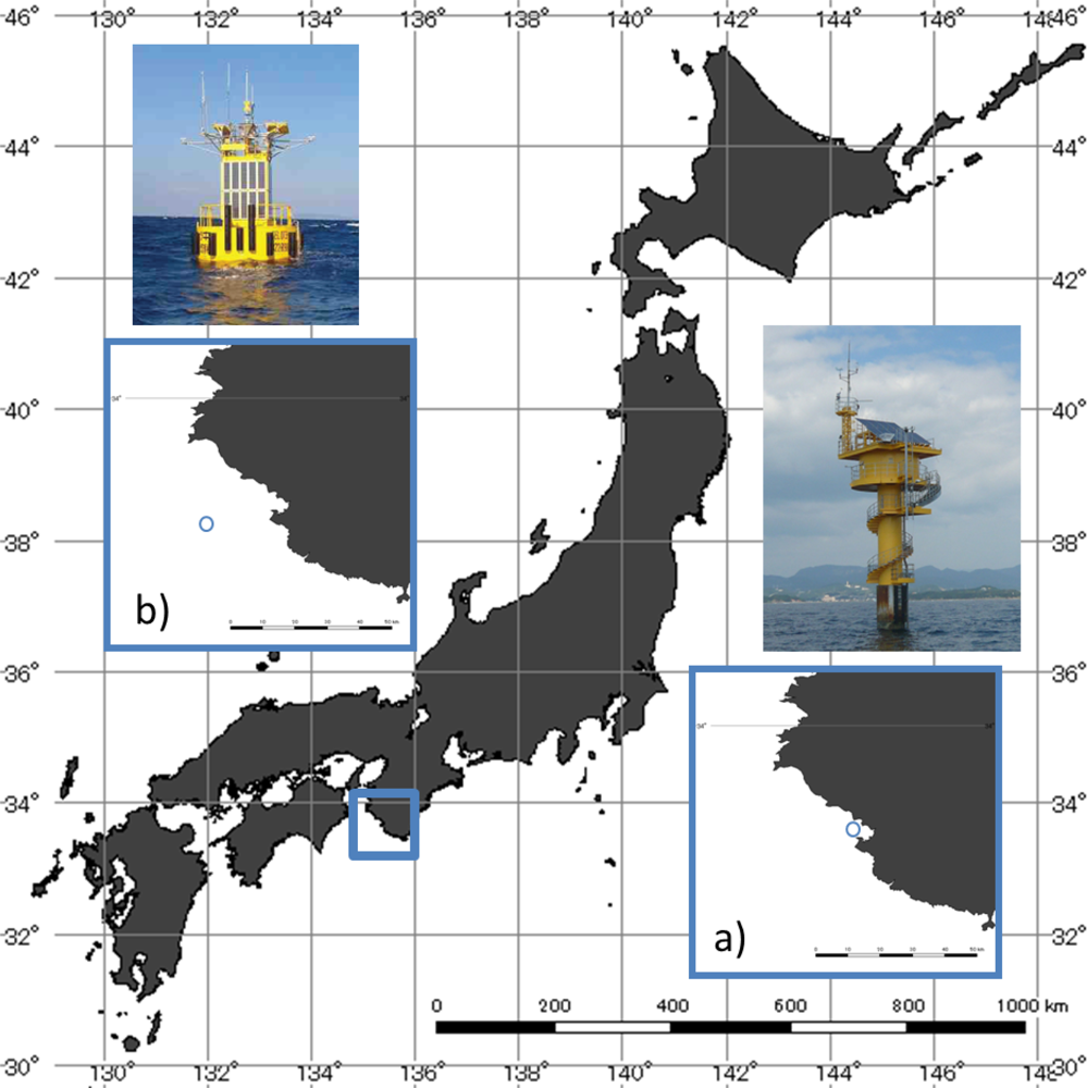
2.1. Target Area and in situ Measurements

The target area of this study is the coastal waters off Shirahama, shown in Figure 1. This area is located in the western part of Japan, including the Kii Channel facing the Pacific Ocean, and known as a relatively windy coastal area in this region, because this channel gives passage to the northwesterly winter monsoon wind. In this area there are two observation sites; the Shirahama offshore platform and the South Wakayama buoy (Hereinafter, SW-buoy). The first one, the Shirahama offshore platform (33°42′32″N, 135°19′58″E) is the oceanographic and meteorological observation station operated by the Disaster Prevention Research Institute, Kyoto University since 1994. On the platform, wind speed and direction are measured at a height of 23 m above mean sea level with a propeller anemometer. This study uses the hourly 10-min averaged wind speed from 2003 to 2011. The second one, the SW-buoy (33°38′32″N, 135°09′24″E) is a buoy for wave observation and is operated by the Ports and Harbors Bureau, Ministry of Land, Infrastructure, Transport and Tourism. On the buoy, wind speed and direction are measured with a propeller anemometer at a height of 7 m. The hourly 10-min averaged wind speed data for two years from 2009 to 2010 is used in this study.

In order to compare the SAR-derived wind speed at 10 m height with in situ measured wind speeds, the in situ wind speeds at 23 m height at Shirahama is corrected to the 10 m-height wind speed. For this height correction, the LKB code [11], which can calculate vertical profile of wind speed based on the Monin-Obukhov similarity theory, is used. Three kinds of inputs; air temperature, relative humidity, and sea surface temperature (SST) are required in the LKB code. The wind profile, which can take the effect of atmospheric stability expressed as Ψ_u(ζ) into account, is shown as

$$u=\frac{u_{*}}{\kappa }\left[\mathit{ln}\hspace{0.17em}\left(\frac{z}{z_0}\right)-{\mathrm{\Psi }}_u\left(\zeta \right)\right]$$

(1)

Here, u_* is frictional velocity, z₀ is roughness length, and κ is the von Karman constant (=0.4). The relation between z₀ and u_* is given as

$$z_0=0.11\frac{\upsilon }{u_{*}}+\alpha \frac{u_{*}^2}{g}$$

(2)

where α is Charnock’s parameter with a value of 0.011 [12], υ is the kinematic viscosity, and g is the acceleration due to gravity. The parameters, z₀ and u_* can be determined iteratively through the Equations (1) and (2) and other equations regarding the stability parameter ζ. In the height correction from 23 m to 10 m, wind speed is decreased by 5% on average. The converted 10 m-height 10-min averaged wind speeds are used as the in situ values for the comparison with the SAR-derived wind speeds.

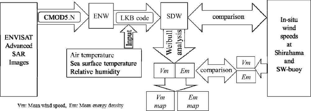
2.2. Derivation of Wind Speed from SAR Image

Figure 2 shows the low chart of how to assess offshore wind resource using SAR images. In-depth descriptions regarding each processing will be given later.

Firstly, this study uses 104 images from the C-band ASAR onboard the ENVISAT satellite, launched by the European Space Agency in 2002. The inventory of the SAR data used here is listed in

Table 1. Inventory of 104 ENVISAT ASAR images used in this study.

Date (year/month/day)	Time (h:min:s)	Ascending or Descending	Observation Mode	Date (year/month/day)	Time (h:min:s)	Ascending or Descending	Observation Mode
20030314	01:06:56	DS	IMP	20100624	12:50:44	AS	WSM
20030418	01:06:59	DS	IMP	20100625	01:06:07	DS	WSM
20030507	01:09:47	DS	IMP	20100627	12:56:29	AS	WSM
20030716	01:09:53	DS	IMP	20100630	13:02:14	AS	WSM
20030801	01:07:05	DS	IMP	20100708	00:57:30	DS	WSM
20030820	01:09:56	DS	IMP	20100710	12:47:52	AS	WSM
20030924	01:09:56	DS	IMP	20100711	01:03:15	DS	WSM
20031010	01:07:04	DS	IMP	20100713	12:53:38	AS	WSM
20031029	01:09:50	DS	IMP	20100724	00:54:39	DS	WSM
20031114	01:07:01	DS	IMP	20100726	12:45:02	AS	WSM
20040123	01:07:00	DS	IMP	20100727	01:00:25	DS	WSM
20040211	01:09:51	DS	IMP	20100730	01:06:10	DS	WSM
20040227	01:07:00	DS	IMP	20100801	12:56:32	AS	WSM
20040507	01:07:00	DS	IMP	20100812	00:57:33	DS	WSM
20040630	01:09:55	DS	IMP	20100814	12:47:55	AS	WSM
20040731	12:48:26	AS	IMP	20100815	01:03:18	DS	WSM
20040820	01:07:04	DS	IMP	20100817	12:53:40	AS	WSM
20040908	01:09:55	DS	IMP	20100818	01:09:03	DS	WSM
20041013	01:09:56	DS	IMP	20100828	00:54:41	DS	WSM
20041029	01:07:06	DS	IMP	20100830	12:45:03	AS	WSM
20041203	01:07:03	DS	IMP	20100831	01:00:26	DS	WSM
20050107	01:06:58	DS	IMP	20100903	01:06:10	DS	WSM
20050211	01:07:01	DS	IMP	20100905	12:56:32	AS	WSM
20050511	01:09:59	DS	IMP	20100916	00:57:32	DS	WSM
20050527	01:07:07	DS	IMP	20100918	12:47:54	AS	WSM
20050701	01:07:09	DS	IMP	20100919	01:03:17	DS	WSM
20050805	01:07:05	DS	IMP	20100921	12:53:38	AS	WSM
20050909	01:07:02	DS	IMP	20100922	01:09:01	DS	WSM
20051014	01:07:05	DS	IMP	20111018	12:58:01	AS	WSM
20051118	01:07:03	DS	IMP	20111019	01:11:12	AS	WSM
20051223	01:06:57	DS	IMP	20111026	13:04:41	AS	WSM
20060111	01:09:42	DS	IMP	20111030	01:07:59	DS	WSM
20060215	01:09:45	DS	IMP	20111106	13:01:28	AS	WSM
20060303	01:06:54	DS	IMP	20111109	12:51:34	AS	WSM
20070829	01:09:47	DS	IMP	20111114	13:08:08	AS	WSM
20071107	01:09:43	DS	IMP	20111125	13:04:54	AS	WSM
20071123	01:06:48	DS	IMP	20111206	13:01:39	AS	WSM
20071208	12:48:10	AS	IMP	20111207	01:14:50	AS	WSM
20071209	01:03:59	DS	IMP	20111209	12:51:45	AS	WSM
20071212	01:09:41	DS	IMP	20111210	01:04:56	DS	WSM
20080112	12:48:12	AS	IMP	20111214	13:08:19	AS	WSM
20080113	01:04:01	DS	IMP	20111217	12:58:25	AS	WSM
20080116	01:09:43	DS	IMP	20111218	01:11:36	AS	WSM
20080131	12:51:01	AS	IMP	20111221	01:01:42	DS	WSM
20080201	01:06:50	DS	IMP	20111228	12:55:10	AS	WSM
20080216	12:48:09	AS	IMP	20120105	13:01:49	AS	WSM
20080217	01:03:59	DS	IMP	20120106	01:15:00	AS	WSM
20080220	01:09:42	DS	IMP	20120108	12:51:55	AS	WSM
20080306	12:51:02	AS	IMP	20120109	01:05:05	DS	WSM
20080307	01:06:51	DS	IMP	20120113	13:08:26	AS	WSM
20080322	12:48:13	AS	IMP	20120116	12:58:33	AS	WSM
20080323	01:04:02	DS	IMP
20080326	01:09:43	DS	IMP

. They include two kinds of images; the Precision Image Product (IMP) and the Wide Swath Mode (WSM). The IMP and WSM images have 12.5 m and 75 m pixel spacing, respectively. But in the preprocessing these SAR images are smoothed to the grids with a 0.005 × 0.005 degree spatial resolution to remove the speckle noise, which is appeared in coherent imaging systems such as SAR.

For deriving wind speed from the SAR image, CMOD5.N [9] is used to derive wind speed from normalized radar cross section (NRCS) represented in the SAR images. The primary equation of CMOD5.N can be written as

$${\sigma }_{vv}^o=b_0{\left(1.0+b_1\hspace{0.17em}\text{cos}\varphi +b_2\hspace{0.17em}\text{cos}\left(2\varphi \right)\right)}^{1.6}$$

(3)

where ${\sigma }_{vv}^0$ is the VV-polarized NRCS obtained from a SAR image, ϕ is the relative wind direction defined as the angle between the radar look direction and true wind direction, and b₀, b₁, and b₂ are the parameters depending on the radar incidence angle and wind speed. Here, it is necessary to acquire values of wind direction from another external data source. Same as [5], this study uses the wind direction obtained from numerical simulation with the mesoscale meteorological model WRF [8]. Details of the WRF simulation are described in Subsection 2.3.

2.3. Conversion from Equivalent Wind Speed (ENW) to Stability-Dependent Wind Speed (SDW)

The output from CMOD5.N is the equivalent neutral wind speed (ENW) [13], which is the wind speed obtained under the assumption of neutral atmospheric stability in the surface layer. Thus, the LKB code [11] is used to convert the ENW to the stability-dependent wind speed (SDW), which is comparable to a true wind speed. Since Takeyama et al.[6] provides an in-depth description of how to calculate SDW from ENW with the LKB code, this paper omits to describe it. What is important is that the LKB code requires three parameters; air temperature, relative humidity, and sea surface temperature (SST) to calculate SDW, and this study obtains these three values from numerical simulation with the mesoscale meteorological model WRF.

The WRF (Weather Research and Forecasting model) [8] is the mesoscale numerical weather prediction system developed by seven institutes in the United States including the National Center for Environmental Prediction (NCEP) and the National Center for Atmospheric Researches (NCAR). In this study, WRF is set up with two domains consisting of 100 × 100 grids with horizontal resolutions of 5 km and 1 km, and 28 vertical layers. As the initial and boundary conditions, 3-hourly (6-hourly before February 2006) 5 km × 5 km (10 km × 10 km before April 2009) mesoscale analysis MANAL provided from Japan Meteorological Agency and daily 0.05° × 0.05° sea surface temperature OSTIA SST provided from Met Office [14] are used in the simulation. WRF is run for 24 h for each SAR image, corresponding to the time of passage of ENVISAT (mostly at 01 and 13 UTC) with two-way nesting, which allows the interaction between the mother and child domains. More in-depth model configuration is shown in

Table 2. Configurations of the mesoscale meteorological model WRF and input data.

		JAM Meso-Analysis (MANAL)
Initial data		5 km × 5 km, 10 km × 10 km (before April 2009)
		3-hourly, 6-hourly (before February 2006)
		Met Office OSTIA SST (0.05° × 0.05°, daily)
Nesting option		two-way nesting
Vertical resolution		28 levels (surface to 100 hPa)
Time period		24 h including the time of passage of ENVISAT
Domain		Domain 1	Domain 2
Horizaontal resolution		5.0 km	1.0 km
Grid points		100 × 100	101 × 101
Time step		30 s	6 s
Physics option	Surface layer	Monin-Obukhov (Janjic Eta)
	Planetary Boundary Layer	MYJ (Eta) TKE
	Short wave radiation	Dudhia
	Long wave radiation	RRTM
	Cloud micropysics	WSM3
	Cumulus parameterization	Kain-Fritsch (new Eta)	none
	Land surface	Five-layer soil
FDDA option		Enable including PBL	Enable excluding PBL

, and the domains used in the WRF simulation are shown in Figure 3. In the previous study [6], a RMSE of the wind direction from the WRF simulation was reported as 25.4° at Shirahama.

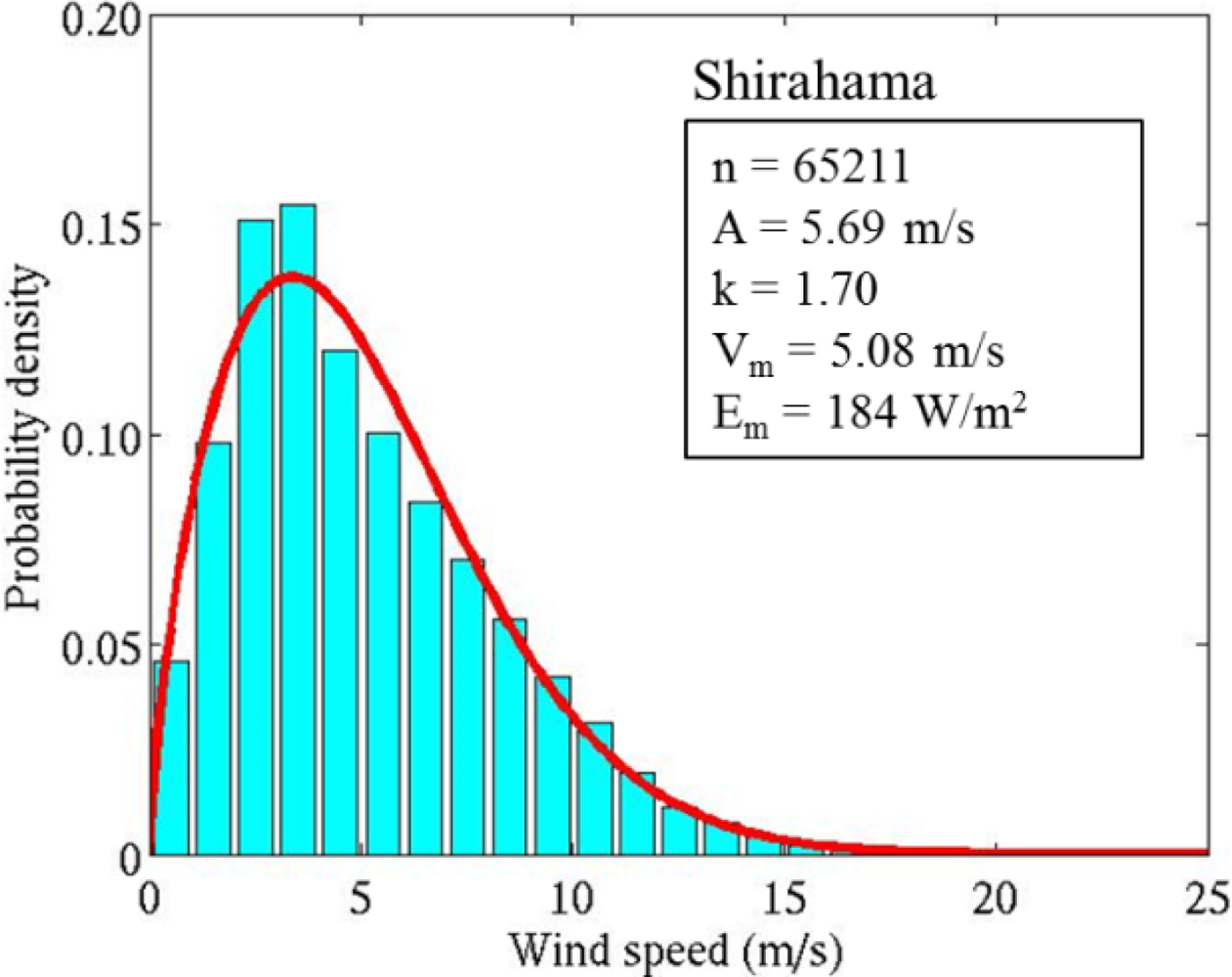
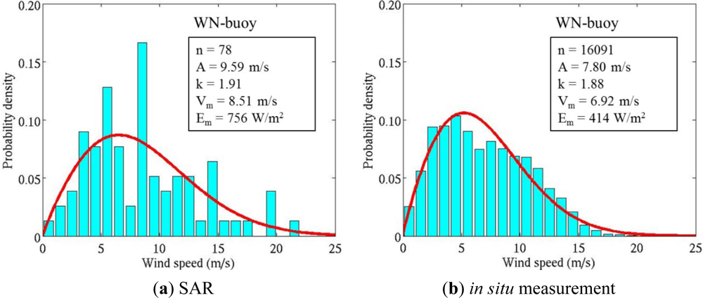
2.4. Application of Weibull Distribution Function

The wind resource assessment using SAR images is normally accompanied with the use of the Weibull analysis. With the Weibull distribution, the probability density function of wind speed f(V) is expressed as the following equation.

$$f\left(V\right)=\frac{k}{A}{\left(\frac{V}{A}\right)}^{k-1}\hspace{0.17em}\mathit{exp}\left[-{\left(\frac{V}{A}\right)}^k\right]$$

(4)

where V is wind speed (m/s), and k and A are called shape and scale parameters, respectively. From the two parameters k and A, mean wind speed V_m can be calculated as follows:

$$V_m=A\mathrm{\Gamma }\left(1+\frac{1}{k}\right)$$

(5)

Here, Γ is the Gamma function defined as

$$\mathrm{\Gamma }\left(1+\frac{1}{k}\right)=\underset{0}{\overset{\infty }{\int }}{t}^{1/k}\hspace{0.17em}{e}^{-t}\hspace{0.17em}dt$$

(6)

The mean wind energy density E_m is shown as

$$E_m=\frac{\rho }{2}{A}^3\mathrm{\Gamma }\left(1+\frac{3}{k}\right)$$

(7)

Here, ρ is air density, which is set to 1.225 (kg/m³) in this study. In the next section, wind resources are evaluated with the mean wind speed V_m and E_m.

3. Results and Discussion

3.1. Accuracy of SAR-Derived Wind Speed and Wind Energy Density

First, the accuracy of the SAR-derived wind speed and wind energy density is examined. Figure 4 shows scatter plots of SAR-derived versus in situ measured wind speeds. In Figure 4, the bias and the root mean square error (RMSE) of the SAR wind speed are 0.52 m/s and 2.33 m/s, respectively. Since the mean in situ wind speed is 4.92 m/s, the relative ratios of the bias and RMSE become 11% and 47%, respectively. The results indicate slightly lower accuracy than those in the previous study [5]. One of the reasons for the lower accuracy is low wind speeds (no more than 2 m/s). In the SAR wind speed retrieval, low wind speeds are usually removed because it is well known that GMFs cannot derive these wind speeds with high accuracy. But, in this study, all ranges of wind speeds are included, because they are necessary for an estimation of the Weibull distribution (shown detail in Section 3.2).

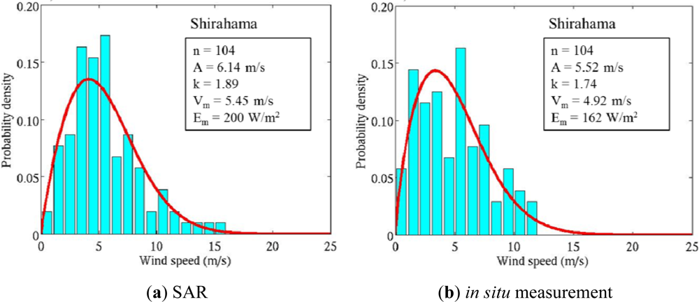
3.2. Comparisons in Terms of Weibull Distribution Function

Figure 5 compares the Weibull distribution for 104 SAR-derived wind speeds at Shirahama with that for corresponding in situ measurements. The scale parameters A are 6.14 (SAR) and 5.52 m/s (in situ), and the shape parameters k are 1.89 (SAR) and 1.74 m/s (in situ). Though the difference of k between them is only 0.15, the difference of A is no less than 0.62 m/s (10%). Meanwhile, mean wind speeds V_m are 5.45 (SAR) and 4.92 m/s (in situ). The difference of V_m is approximately 10%, indicating that the SAR-derived mean wind speed is higher than the in situ measurement. The tendency of the overestimation becomes more remarkable in mean wind energy density E_m. The energy density E_m estimated from the SAR-derived and in situ measured wind speeds exhibits 200 W/m² and 162 W/m², respectively. The SAR-derived E_m is 24% larger than in situ E_m.

In the next step, the V_m and E_m estimated from SAR images are compared with those from long-term in situ measurement (2003 through 2011) at Shirahama in Figure 6. It is firstly confirmed that the differences in both V_m and E_m between Figures 6 and 5(b) are only 0.16 m/s and 22 W/m² and little differences can be seen. This means that the 104 samples well represent characteristics of the long term wind climate. Accordingly, results from the comparison of Figure 5(a) with Figure 6 are similar to those with Figure 5(b). That is, the SAR-estimated V_m in Figure 5(a) (5.45 m/s) is 1.07 times higher than the long-term mean shown in Figure 6 (5.08 m/s). As for mean wind energy density E_m, the SAR-estimated value is 1.09 times larger than the long-term mean.

Meanwhile, Figure 7 compares two Weibull distributions based on SAR and in situ measurements at SW-buoy. At the buoy, 78 SAR images and 16,091 wind speed measurements are used for the comparison. In contrast to Shirahama, the accuracy of the SAR-estimated V_m is not good at SW-buoy, and the SAR-estimated V_m is 8.51 m/s against the in situ long-term mean of 6.92 m/s. The difference is 23% (1.59 m/s), meaning 1.23 times as large as the in situ V_m. The ratio is slightly larger than that at Shirahama (1.07). Additionally, the mean wind energy density E_m is 756 W/m² for SAR and 414 W/m² for in situ measurement, indicating a large overestimation probably due to the lack of samples, as speculated in the introduction.

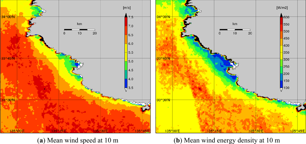
3.3. Wind Resources in Coastal Waters off Shirahama

The final purpose of this study is to present wind resource maps in the coastal waters off Shirahama. It is desirable that the wind resource maps will be made as accurately as possible, even if the SAR-derived wind speed has been found to have errors. Then, an attempt is made to use in situ measurements to improve the SAR-derived wind speed fields. As shown in the previous section, the ratio of the SAR-derived mean wind speed to the in situ long-term average is 1.07 and 1.23 at Shirahama and SW-buoy, respectively. Here, the ratio at Shirahama (1.07) can be considered as a more reliable value, because the two ratios are obtained based on in situ measurements for about 8 years at Shirahama and 2 years at SW-buoy, as well as they are based on 104 and 78 SAR images at Shirahama and SW-buoy, respectively. Thus, the ratio of 1.07 is adopted to correct the tendency of the overestimation and all the SAR wind speeds are divided by 1.07. Then, mean wind speed V_m and mean energy density E_m are calculated at all pixels of the SAR image by using the Weibull distribution function. Wind resource maps presented hereinafter show the wind speed after this correction.

Figure 8 shows spatial distributions of the SAR-estimated mean wind speed V_m and mean wind energy density E_m at the height of 10 m. It is clearly found that there is a band-like area with strong winds extending from northwest to southwest roughly 20 to 40 km off the coast of Shirahama. Toward the strong wind axis, mean wind speed changes from 3.5 m/s along the coast to nearly 7.5 m/s. The wind energy density ranges from 100 W/m² along the coast line to 550 W/m² near the strong wind axis. Qualitatively, characteristics of the distributions seem to be reasonable and are similar to the map made with WRF in the previous study [15].

Finally, to make wind resource maps at a typical hub height of 80 m, the mesoscale model WRF is used to calculate vertical wind speed ratios between 10 m and 80 m (U₈₀/U₁₀) at each pixel for 104 SAR images. One example of the distribution of the ratio U₈₀/U₁₀ is shown in Figure 9. The value normally ranges from nearly 1.0, which corresponds to very unstable atmospheric conditions, to 1.4 in stable conditions. The obtained mean wind speed and mean wind energy density at the height of 80 m are represented in Figure 10. It is found that mean wind speed is around 5.0 m/s near the coast of Shirahama, increasing up to nearly 9.0 m/s about 30 km off Shirahama. In terms of mean wind energy density at 80 m height, it is found that the Shirahama offshore platform is located in a weak wind region with wind energy density of 250 W/m², and that the maximum wind energy density of more than 800 W/m² is located about 30 km to the southwest or west-southwest of the Shirahama offshore platform. The offshore wind resource maps created here will be helpful in the future for development of floating offshore wind farms in the coastal waters.

4. Conclusions

In this study, 104 ENVISAT ASAR images were used to make maps of offshore wind resource in the coastal waters off Shirahama. The geophysical model function CMOD5.N was used to derive wind speed from the SAR images, and the mean wind speed and wind energy density were estimated using the Weibull distribution function. These accuracies were discussed in comparison with in situ measurements from the Shirahama offshore platform (referred to as Shirahama) and the Southwest Wakayama buoy (SW-buoy).

Conclusions in this study are summarized as follows.

(1)

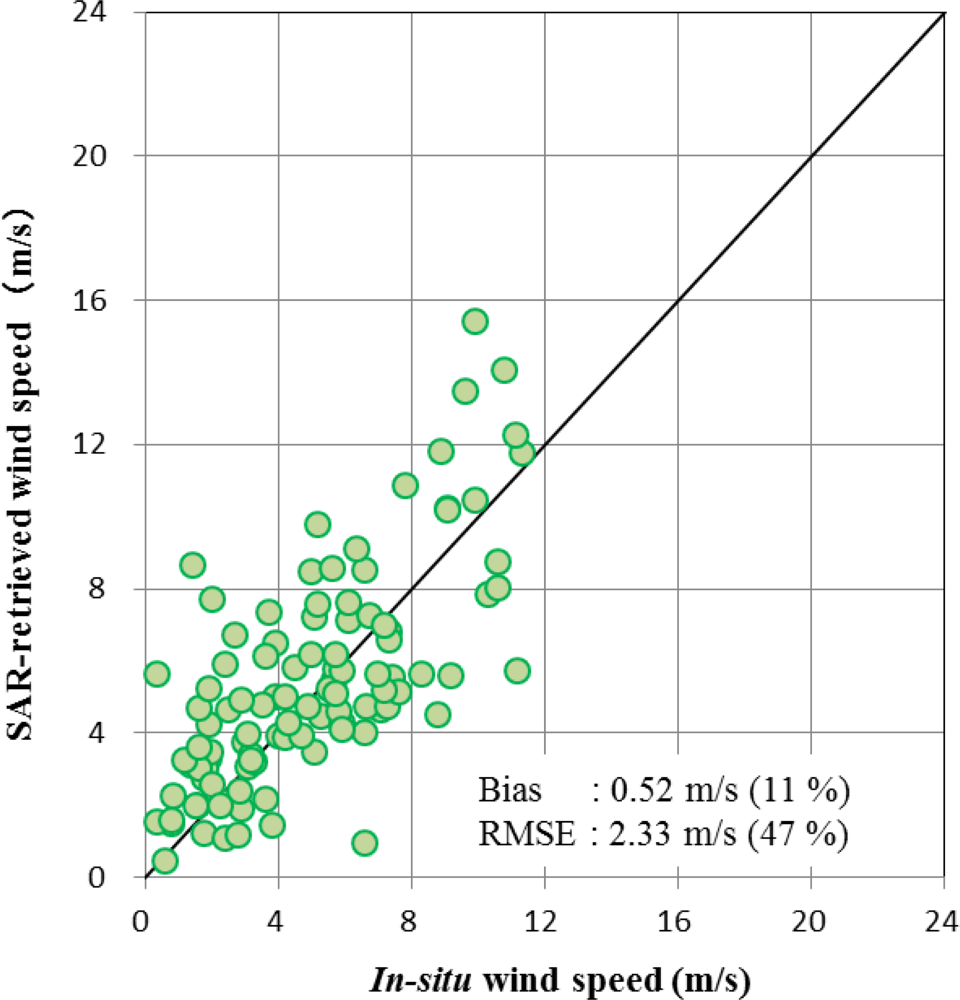
Compared with in situ measurements at Shirahama, the SAR-derived 10 m-height wind speed had a bias of 0.52 m/s (11% of in situ mean wind speed) and a RMSE of 2.33 m/s (47%).

(2)

The mean wind speed and energy density estimated from SAR images with the Weibull distribution function are 5.45 m/s and 200 W/m² at Shirahama, and 8.51 m/s and 756 W/m² at SW-buoy. It is found that the 104 SAR images overestimates the wind resources at both sites, compared to those from long-term in situ wind speed measurements. At Shirahama, SAR overestimates mean wind speed by 7% compared to the long-term in situ average.

(3)

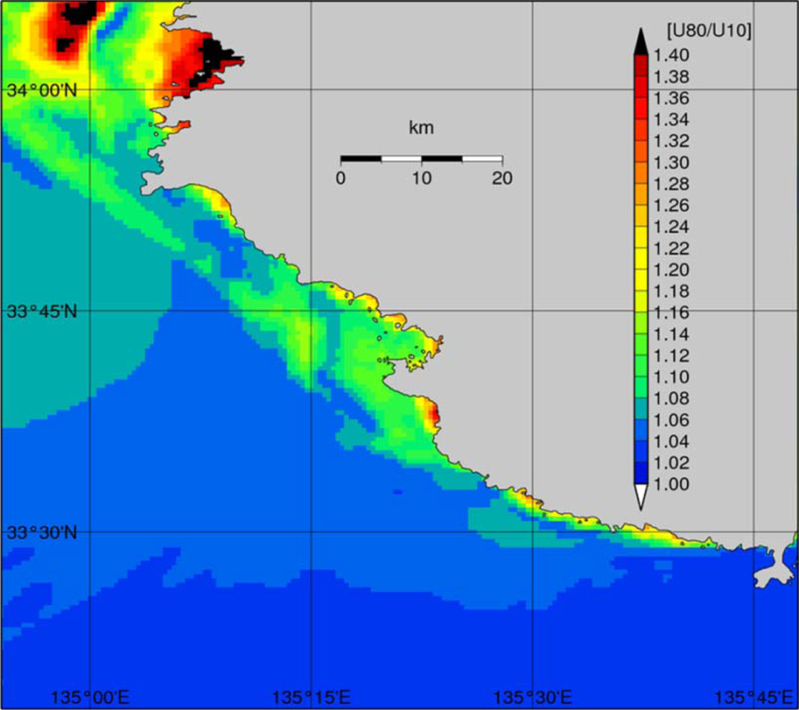
In order to obtain more reliable mean wind speed and wind energy density maps, the accuracy of the SAR derived wind speeds was improved by making a long-term bias correction. Then, using the 10 m-height wind speed together with the ratio between 10 m- and 80 m-height wind speeds calculated from the mesoscale meteorological model WRF, mean wind speed and wind energy density maps at 80 m height were made and presented at the end of the paper.

Further work is necessary to increase the accuracy of the maps by combining them with information from remote sensing measurements by satellite-borne scatterometers and radiometers and simulation results from a mesoscale model, as well as by increasing the number of SAR images used in the analysis.

References

1. Hasager, C.B.; Badger, M.; Peña, A.; Larsén, X.G.; Bingöl, F. SAR-based wind resource statistics in the Baltic Sea. Remote Sens. 2011, 3, 117–144. [Google Scholar]
2. Christiansen, M.B.; Koch, W.; Horstmann, J.; Hasager, C.B.; Nielsen, M. Wind resource assessment from C-band SAR. Remote Sens. Environ. 2006, 105, 68–81. [Google Scholar]
3. Hasager, C.B.; Dellwik, E.; Nielsen, M.; Furevik, B.R. Validation of ERS-2 SAR offshore wind-speed maps in the North Sea. Int. J. Remote Sens. 2004, 25, 3817–3841. [Google Scholar]
4. Kozai, K.; Ohsawa, T.; Shimada, S.; Takeyama, Y.; Hasager, C.B.; Badger, M. Comparison of Envisat/ASAR-Estimated Offshore Wind Resource Maps around Shirahama with Those from Mesoscale Models MM5 and WRF. Proceedings of European Offshore Wind 2009, Stockholm, Sweden, 14–16 September 2009; p. 7.
5. Takeyama, Y.; Ohsawa, T.; Kozai, K.; Hasager, C.B.; Badger, M. Effectiveness of WRF wind direction for retrieving coastal sea surface wind from synthetic aperture radar. Wind Energy 2012. [Google Scholar] [CrossRef]
6. Takeyama, Y.; Ohsawa, T.; Kozai, K.; Hasager, C.B.; Badger, M. Comparison of geophysical model functions for SAR wind speed retrieval in Japanese coastal waters. Remote Sens. 2013, 5, 1956–1973. [Google Scholar]
7. Kozai, K.; Ohsawa, T.; Takahashi, R.; Takeyama, Y. Estimation Method for Offshore Wind Energy Using Synthetic Aperture Radar and Weibull Parameters. Proceedings of the Nineteenth 2009 International Offshore and Polar Engineering Conference (ISOPE), Osaka, Japan, 21–26 June 2009; pp. 419–423.
8. Skamarock, W.C.; Klemp, J.B.; Dudhia, J.; Gill, D.O.; Barker, D.M.; Wang, W.; Powers, J.G. A Description of the Advanced Research WRF Version 3; NCAR Technical Notes, TN-475+STR. Mesoscale and Microscale Meteorology Division, National Center for Atmospheric Research: Boulder, CO, USA, 2008; p. 113. Available online: http://www.mmm.ucar.edu/wrf/users/docs/arw_v3.pdf (accessed on 2 April 2013).
9. Hersbach, H. Comparison of C-band scatterometer CMOD5.N equivalent neutral winds with ECMWF. J. Atm. Ocean. Tech. 2010, 27, 721–736. [Google Scholar]
10. Barthelmie, R.J.; Pryor, S.C. Can satellite sampling of offshore wind speeds realistically represent wind speed distributions? J. Appl. Meteor. 2003, 42, 83–94. [Google Scholar]
11. Liu, W.T.; Katsaros, K.B.; Businger, J.A. Bulk parameterization of air-sea exchanges of heat and water vapor including the molecular constraints at the interface. J. Atmos. Sci. 1979, 36, 1722–1735. [Google Scholar]
12. Charnock, H. Wind stress on a water surface. Quart. J. R. Meteorol. Soc. 1955, 81, 639–640. [Google Scholar]
13. Liu, W.T.; Tang, W. Equivalent Neutral Wind; JPL Publication 96-17. NASA: Pasadena, CA, USA, 1996. Available online: http://airsea-www.jpl.nasa.gov/publication/paper/Tang-Liu-1996-jpl.pdf (accessed on 2 April 2013).
14. Operational Sea Surface Temperature and Sea Ice Analysis (OSTIA) SST. Available online: http://ghrsst-pp.metoffice.com/pages/latest_analysis/ostia.html (accessed on 10 November 2012).
15. Shimada, S.; Ohsawa, T. Accuracy and characteristics of offshore wind speeds simulated by WRF. SOLA 2011, 7, 21–24. [Google Scholar]
Figure 1. Locations of the coastal waters off Shirahama. Circle in the small maps indicates (a) the Shiraham offshore platform and (b) the Southwest Wakayama buoy (SW-buoy).
Remotesensing 05 02883f1
Figure 2. Flow chart of wind resource estimation from ASAR images and their comparison with in situ measurements.
Remotesensing 05 02883f2
Figure 3. Domains used in the WRF simulation.
Remotesensing 05 02883f3
Figure 4. Scatter plots of SAR-derived versus measured wind speeds at Shirahama.
Remotesensing 05 02883f4
Figure 5. Comparison of Weibull distributions between (a) SAR-derived and (b) in situ measured wind speeds at Shirahama.
Remotesensing 05 02883f5
Figure 6. Weibull distributions from long-term in situ measured wind speeds (2003 through 2011) at Shirahama.
Remotesensing 05 02883f6
Figure 7. Comparison of Weibull distributions between (a) SAR-derived and (b) in situ wind speeds at SW-buoy.
Remotesensing 05 02883f7
Figure 8. Spatial distributions of (a) mean wind speed Vm and (b) mean wind energy density Em at 10 m height in the coastal waters off Shirahama.
Remotesensing 05 02883f8
Figure 9. An example of the distribution of the ratio U80/U10 at 9 September 2005.
Remotesensing 05 02883f9
Figure 10. Spatial distribution of (a) mean wind speed Vm and (b) mean energy density Em at 80 m height in the coastal waters off Shirahama.
Remotesensing 05 02883f10