Abstract
Vegetation phenology plays an important role in regulating processes of terrestrial ecosystems. Dynamic ecosystem models (DEMs) require representation of phenology to simulate the exchange of matter and energy between the land and atmosphere. Location-specific parameterization with phenological observations can potentially improve the performance of phenological models embedded in DEMs. As ground-based phenological observations are limited, phenology derived from remote sensing can be used as an alternative to parameterize phenological models. It is important to evaluate to what extent remotely sensed phenological metrics are capturing the phenology observed on the ground. We evaluated six methods based on two vegetation indices (VIs) (i.e., Normalized Difference Vegetation Index and Enhanced Vegetation Index) for retrieving the phenology of temperate forest in the Agro-IBIS model. First, we compared the remotely sensed phenological metrics with observations at Harvard Forest and found that most of the methods have large biases regardless of the VI used. Only two methods for the leaf onset and one method for the leaf offset showed a moderate performance. When remotely sensed phenological metrics were used to parameterize phenological models, the bias is maintained, and errors propagate to predictions of gross primary productivity and net ecosystem production. Our results show that Agro-IBIS has different sensitivities to leaf onset and offset in terms of carbon assimilation, suggesting it might be better to examine the respective impact of leaf onset and offset rather than the overall impact of the growing season length.
1. Introduction
Vegetation phenology, or the timing of plant growth stages (e.g., the timing of budburst, flowering, leaf coloring), is considered a robust indicator of short-term climate variation and long-term climate trends because it is driven by environmental factors, such as temperature, precipitation and photoperiod. Vegetation phenology has received increased attention recently because evidence from ground observations as well as satellite remote sensing has shown that vegetation phenology has shifted during the past few decades [1–5], especially at middle and high latitudes of the Northern Hemisphere, as a result of increasing average temperature [6,7]. On the other hand, shifts in vegetation phenology can exert strong control on the feedbacks between the biosphere and atmosphere by affecting biogeochemical processes (e.g., exchange of carbon dioxide, production of biogenic volatile organic compounds) and biophysical properties (e.g., seasonal variation in albedo) of ecosystems [8,9]. Bias in vegetation phenology therefore may lead to errors in carbon and water exchange and energy budgets simulated in dynamic ecosystem models (DEMs) [10] as well as climate patterns simulated in coupled global climate models (GCMs) [11].
A multi-model synthesis study has shown that vegetation phenology is poorly represented in many terrestrial biosphere models [10], which highlighted the urgency of improving phenological models embedded in DEMs. Phenological models can potentially be improved by reducing the uncertainties that stem from model structure, model parameters, or drivers [12]. For example, a comprehensive comparison of existing phenological models across geographic zones may help reduce the structural uncertainties [13]. Moreover, modeling studies at the regional scale demonstrated that, due to the difference in species type and composition, forests at different locations do not share common parameters, such as base temperature for growing degree day (GDD) calculation [13,14]. Thus, location-specific parameterization has the potential to reduce the uncertainty associated with model parameters. Parameterization of phenological models at a specific location requires corresponding phenological observations. As ground-based phenological observations are limited in spatial coverage and quantity, phenology derived from remote sensing becomes the only alternative when parameterization over a large continuous area is needed.
Phenology derived from remote sensing, which has recently been referred to as land surface phenology (LSP) in order to distinguish it from in situ monitoring at species level, has long been used to examine phenological changes [2,4,5,15–17] and to develop large-scale phenology models [18,19]. Numerous remote sensing methods, such as vegetation index threshold and curve fitting, have been developed to extract phenological metrics that describe particular timing related to leaf behaviors and photosynthetic activities [19–25]. Start of season (SOS) and end of season (EOS) [22,26], or onset and offset [19] are two phenological phases (i.e., phenophases) most commonly extracted due to their importance in determining the growing season length (GSL). Some studies also derive more than two phenophases. For example, Zhang et al. extracted four phenophases including the onset of greenup, maturity, senescence and dormancy [25]. Most of the methods used to extract phenological metrics are based purely on time series of the normalized difference vegetation index (NDVI) [19,23] and enhanced vegetation index (EVI) [22,25] from various sensors (e.g., Advanced Very High Resolution Radiometer (AVHRR), Moderate-Resolution Imaging Spectroradiometer (MODIS)).
Although phenological metrics derived using different methods share the same name (e.g., SOS), they could actually represent different phenological stages (e.g., the timing when vegetation starts to green up, the timing when vegetation grows the fastest). An intercomparison of SOS retrieved using 10 satellite methods shows that the difference between individual methods can be as much as two months; and two methods were more closely related to ground observations than other methods [27]. Although validation against ground observations has been conducted for remotely sensed phenological metrics in many studies [5,13,14,26,27], the validation process is not standardized because the phenology-monitoring method usually varies among sites, and even the same dataset can be processed differently. More importantly, remotely sensed phenological metrics have not been evaluated in the context of DEMs. In order to improve the accuracy of carbon and water budgets derived from DEMs, there is still a need to define and test phenology transition periods as estimated by satellite sensors [28]. Many issues therefore need to be addressed to determine whether a phenological metric can be used as prescribed phenology in a DEM or to parameterize the embedded phenological model. For example, it should be ensured that the choice of phenology references from available ground observations, against which the remotely sensed phenological metrics would be evaluated, represent the phenology requirements in a DEM. Otherwise, even if the remotely sensed phenological metrics are able to capture some ground phenological metrics that is selected based on the needs of certain applications, they may not be the appropriate variable to be used in a DEM. Remotely sensed phenological metrics depend not only on the method, but also the data source. When the remote sensing data source changes (i.e., from AVHRR to MODIS), a given method may lose its validity due to the difference between sensors, such as spectral and spatial resolution.
In this study, we evaluate phenological metrics derived using six satellite methods for temperate deciduous trees in the context of a DEM, Agro-IBIS (the Integrated Biosphere Simulator, agricultural version) [29–31], using the long-term phenological observations [32] and flux measurements at the Harvard Forest AmeriFlux site [33]. We aim to establish a systematic evaluation process that can be used for the parameterization of phenology models embedded in DEMs. First, we identify the reference phenological metrics from ground observations according to the definition of phenology in the Agro-IBIS model, and use them as prescribed phenology to assess how well Agro-IBIS captures the seasonal evolution of LAI and carbon cycle components. Second, we compare phenological metrics derived from remote sensing with the ground reference. Then, all phenological metrics are used to parameterize the phenology models to examine the propagation of errors during the parameterization and modeling process. Finally, the modeled phenology is used in Agro-IBIS to evaluate the sensitivity of simulated carbon cycle to phenology.
2. Method and Material
2.1. Agro-IBIS Model Description
Agro-IBIS is an improved version of the IBIS DEM [29,31], with the capability to represent both natural and managed ecosystems [30]. The model was developed to simulate the rapid biophysical processes and long-term ecosystem dynamics in response to environmental drivers. It has been evaluated within forests at local and regional scales [34,35], and has been used for many applications such as the quantification of trends in net primary productivity in the 20th century [36] and climate regulation services of ecosystems throughout the Western Hemisphere [37]. The model is designed with a hierarchical conceptual framework, and includes several sub-models (e.g., land surface module, vegetation dynamic module, soil biogeochemistry module) that are capable of simulating vegetation canopy physics, vegetation phenology, soil physics and hydrology, and ecosystem biogeochemistry.
Agro-IBIS has two critical phenophases for natural vegetation—leaf onset and leaf offset. For temperate deciduous trees, leaf onset and offset are defined as the date when LAI starts to increase from a minimum value, and the date when LAI starts to decrease from the peak value, respectively. The model originally used a simple scheme in which leaf onset and offset were both triggered by a critical temperature threshold [29]. Currently, the phenology model is modified from the algorithm developed in literature [19], which is based on GDD for leaf onset and the combination of photoperiod and temperature threshold for leaf offset. An evaluation study at three AmeriFlux sites showed that both schemes had poor performance in representing the phenology at the individual site level; simulated leaf onset dates were generally earlier than the observations with biases up to seven weeks, which led to large errors in canopy structure, such as canopy height and maximum LAI, and in turn the carbon and water exchange [34]. Evaluation at the regional scale showed relatively good performance in capturing the LAI evolution in the northern portion of U.S. eastern deciduous forest; however, earlier onsets were also found in the southern portion, which might be a result of the single threshold of GDD used in the model [35]. While the regional evaluation supports the argument that parameters of phenological models may vary with geographic location [14], the local evaluation implies that the applicability of parameters may change with spatial scale (e.g., from continental scale to site scale).
2.2. Evaluation of Ground Phenology Observations
Harvard Forest is a mixed forest dominated by red maple (Acer rubrum) and red oak (Quercus rubra), both of which are cold-deciduous trees. Harvard Forest is one of few sites that report continual phenology observations for a relatively long period. Spring phenology has been observed since 1990 for 33 species (reduced to nine after 2002). Autumn phenology observations started in 1991 and were reduced to 14 species in 2002 [32]. Spring phenology is recorded as three metrics—percentage of buds on the tree that have broken open (BBRK), percentage of leaves on the tree that are at least 75% of their total size (L75), and percentage of leaves on the tree that are greater or equal to 95% of their final size (L95). Autumn phenology is recorded as the percentage of leaves remaining on the tree that have changed color (LCOLOR), and the percentage of leaves that have fallen (LFALL).
For our Agro-IBIS runs, we used observations from the dominant species (i.e., red maple and red oak) to characterize the temperate deciduous tree plant functional type (PFT). Following literature [13], each metric was fitted for each individual tree sample (multiple tree samples are observed for each species) to a logistic function. We calculated the Day of Year (DOY) when the fitted metrics reached particular amplitude between minimum and maximum at an interval of 10% from 10%–90% (e.g., DOY when 20% of buds have broken denoted by BBRK20, DOY when 30% of leaves have changed color denoted by LCOLOR30). Then, the average DOY of five red maple individuals and four red oak individuals was used to represent the phenology of the site.
We ran a series of Agro-IBIS simulations at the Harvard Forest AmeriFlux site (42.5378°N, 72.1715°W) to determine which observation-based phenological metrics best represent the leaf onset and offset, and how well the model simulates carbon exchange with those metrics. Simulations were conducted with spring onset and autumn offset prescribed as each combination of the observation-based phenological metrics (e.g., BBRK20 as the onset and LCOLOR20 as the offset). We drove the model with a high-resolution (5 min latitude/longitude grid, ~9 km on a side) historical climate dataset created by ZedX Inc. (Bellefonte, PA, USA), which contains daily values of the six variables required by the Agro-IBIS model—maximum and minimum air temperature, precipitation, incoming shortwave radiation, relative humidity and wind speed, over the conterminous U.S. for the period 1948–2007. More detailed information about the dataset can be found in [38]. Data from the grid cell containing the Harvard Forest AmeriFlux site were used to drive Agro-IBIS. The area where phenology is observed (42.53°N–42.54°N, 72.18°W–72.19°W) is approximately 1 km away from the Harvard Forest AmeriFlux site; however, both the phenology observation and the AmeriFlux site are located within the same grid cell of the climate dataset. We therefore assume that there was no variability in phenology within the grid cell. For each simulation, a soil spin-up was conducted so that soil carbon reached near equilibrium. Then the model was run over the period 1948–2007 with phenology simulated using the embedded phenology module for 1948–1990 and prescribed for 1991–2007. We compared the LAI simulated in Agro-IBIS with the deciduous overstory LAI (i.e., LAI of deciduous canopy without the effect of stems, calculated as the overall LAI measured minus the lowest LAI value during the time when no leaves exist) at the Harvard Forest AmeriFlux site. LAI measurements were taken in 1998, 1999, 2005, 2006, 2007 and 2008. Data from 2005 and 2008 were not included because the measurement records are too few in 2005 (only four) and 2008 was beyond the time period of our climate dataset. We calculated the mean percentage error (MPE) between simulated and observed LAI for each simulation. The combination of spring onset and autumn offset metrics, with which the Agro-IBIS model had the best performance in simulating the LAI (i.e., the lowest MPE), was chosen as the ground reference to evaluate the remotely sensed phenological metrics. We also compared simulated annual average gross primary productivity (GPP), ecosystem respiration (Re) and net ecosystem production (NEP) with the gap-filled (Version 7, Level 2) eddy covariance measurements [39].
2.3. Evaluation of Remotely Sensed Phenological Metrics
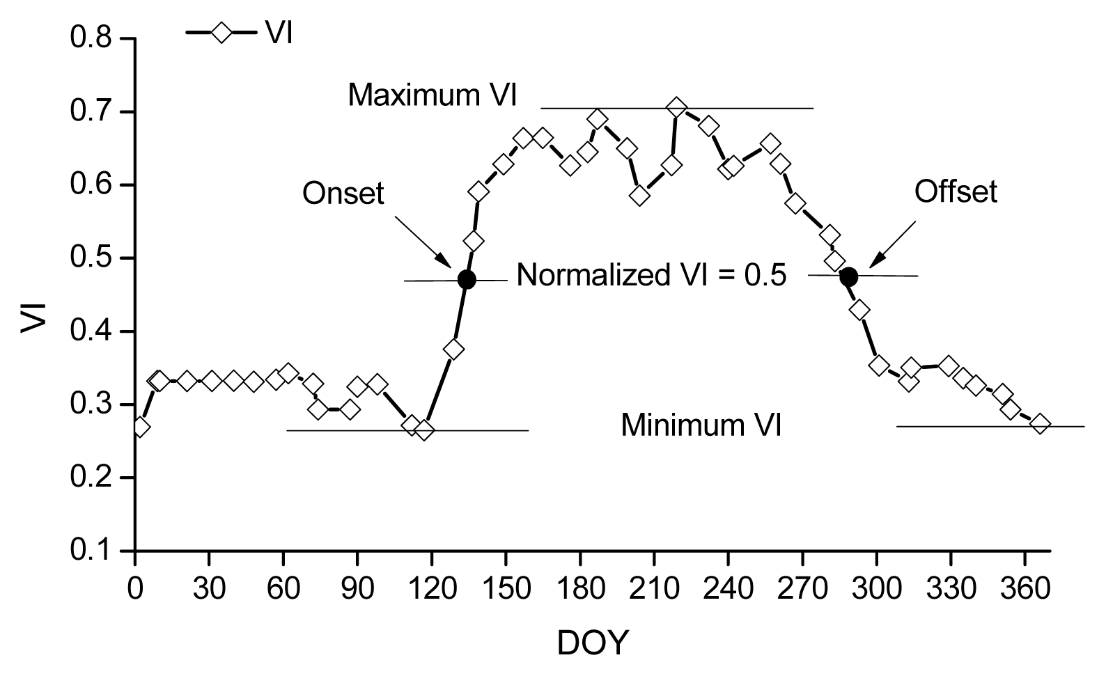
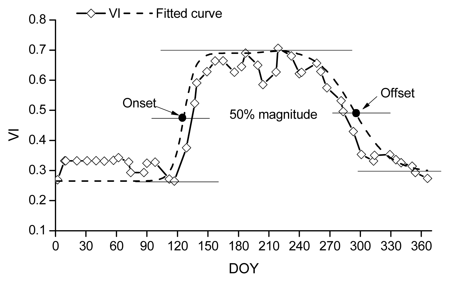
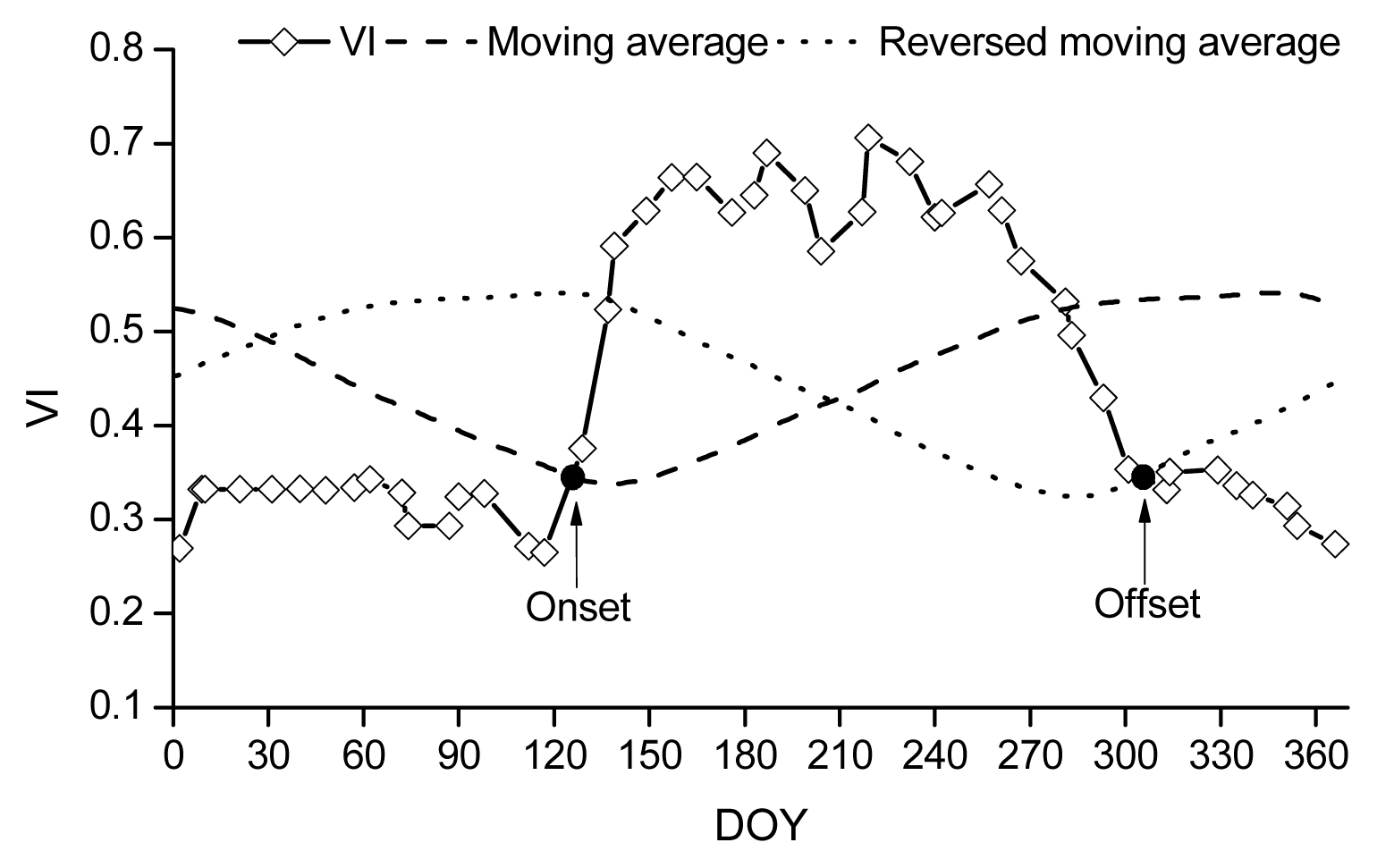
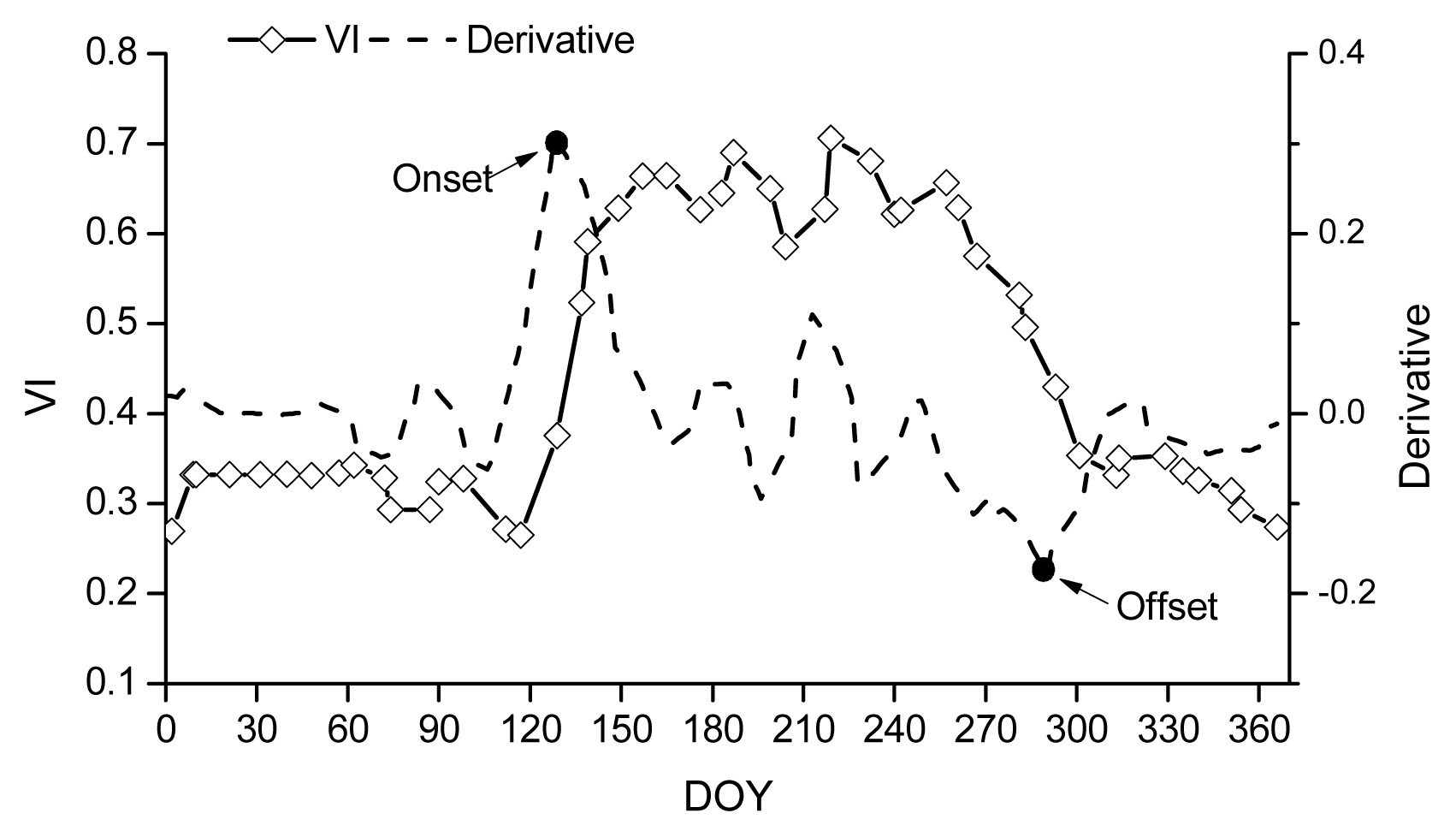
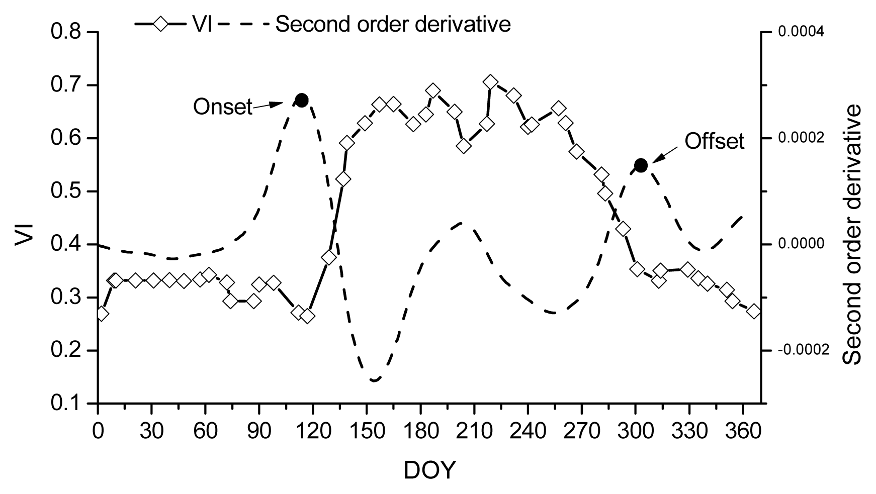
We used six VI-based methods to extract onset and offset dates. A brief description of each method is listed in Table 1. Although some previously published methods used EVI (e.g., [25]), and other methods used NDVI (e.g., [19]), we tested all methods with both VIs. NDVI and EVI were calculated following Equations (1) and (2), respectively, using the eight-day 500 m MODIS surface reflectance product (code: MOD09A1) acquired from the USGS website [40].

Table 1.
Description of the remote sensing methods for retrieving phenology.
where ρNIR, ρRED and ρBLUE are surface reflectance in the near-infrared, red, and blue bands, respectively, and L = 1, C1 = 6, C2 = 7.5, and G (gain factor) = 2.5.
Because phenology derived from different data products could produce different results even if the same method were applied [28], we compared phenology derived from the MOD09A1 product with that derived from the 16-day vegetation indices product (code: MOD13A1; Figure S1 and Tables S1 and S2 in Supplementary Material) and eight-day nadir BRDF-adjusted reflectance (NBAR) product (code: MCD43A4; Figure S2 and Tables S3 and S4 in Supplementary Material), both also having a spatial resolution of 500 m. MOD09A1 showed the best performance (i.e., with inter-annual variability, which is consistent with [28]), therefore we only show results from MOD09A1 for the remainder of this paper. We included in our comparison the land surface dynamic product (code: MCD12Q2), which was derived using one of the methods evaluated here (i.e., LOGISTIC1, Table 1), but with NBAR EVI as input, in order to show how different data sources may affect the results.
We did not consider the quadratic model [21], which involves temperature, because it is fundamentally different from the nonlinear fitting methods purely based on VI and sometimes fails to capture the offset. Methods based on arbitrary thresholds such as NDVI0.2 and NDVI0.3 [27] (i.e., 0.2 and 0.3 were used as NDVI threshold to determine onset) were also excluded, because the difference between sensors could yield large discrepancies in the range of VIs. Our preliminary investigation showed that the MODIS NDVI at our site is sometimes larger than 0.3 over the entire course of a year, which makes it impossible to determine the phenological dates.
In order to derive the phenological metrics, we first applied an algorithm based on the Savitzky-Golay Filter with band quality files and state flags to smooth the VI time series [41]. Then, the reconstructed VI time series were fitted using logistic functions for LOGISTIC1 and LOGISTIC2 method. Before applying the other methods, the smoothed VI time series were interpolated to daily values using a linear model. Dates of onset and offset for 2000–2010 were derived using each method for the five MODIS pixels that are encompassed in the phenology-observation area. The phenological dates averaged across the five pixels were compared with the metrics based on ground observations selected in Section 2.2. The performance of each metric was evaluated using the root mean square deviation (RMSD, Equation (3)) and Spearman’s rank correlation coefficient (ρ). RMSD describes how close remotely sensed phenological metrics are to ground observations, while the correlation coefficient describes how well the remotely sensed phenological metrics capture the inter-annual variability.
where DOYeva is the phenological date to be evaluated, DOYref is the reference phenological metric, and N is the sample size.
2.4. Evaluation of the Propagation of Bias in Phenology
The onset and offset dates derived using different methods with satellite data in Section 2.3 were used to parameterize an onset model [42] (referred to as the “Sequential” model hereafter) and an offset model [43] (referred to as the “Delpierre” model hereafter). The “Sequential” model assumes that leaf onset is triggered when a critical GDD threshold is exceeded after a chilling requirement is fulfilled (Equation (4)). The “Delpierre” model assumes that both temperature and photoperiod control the senescence process (Equation (5)). We chose the “Delpierre” model because it has been proven to have relatively good performance [13]. Although several model structures are available for the onset, we only use the “Sequential” model, which has moderate complexity in terms of parameter number, as an example to show the propagation of bias in phenology. Tests of the “Spring Warming” [44] and “Parallel” models [45] did not change our conclusion and results are not shown.
where xt is the temperature at time t; Rc is the rate of chilling (day); Tchill is base temperature (°C) required by chilling accumulation process; Sc is the accumulated chilling units (day); Ctotal is the critical threshold of the chilling process (day); Rf is the rate of heat forcing (degree-day); Tbase is the base temperature (°C) required by the heat accumulation process; Sf is the accumulated heat forcing units (degree-day); t0 is the starting date of accumulation (DOY); th is the date when the chilling accumulation is completed (DOY); tb is the date of onset (DOY); F* is the critical threshold of heating process (degree-day); P(t) is the photoperiod for day t (hour); Pstart is the photoperiod threshold for offset process (hour); Roff is the rate of forcing for offset process (°C hour hour−1 day−1); Soff is the accumulated forcing units for offset (°C hour hour−1); a and b are parameters of the “Delpierre” model; and Ycrit is the critical threshold of the offset process (°C hour hour−1).
Data used to drive the phenology models include daily temperature (taken here from the ZedX dataset) and photoperiod, which is calculated as a function of latitude and DOY [46]. A simple genetic algorithm written in Interactive Data Language [47] was applied to optimize the model parameters by minimizing the RMSD between the modeled and remotely sensed phenological dates. Convergence was achieved when RMSD could no longer be reduced or 100 generations of parameters were reached. All the parameters of the phenological models were optimized (i.e., Tchill, Ctotal, Tbase, and F* for the “Sequential” model; Pstart, Tchill, a, b, and Ycrit for the “Delpierre” model). Data from the period of 2000–2007, which is the overlap between the references (i.e., remotely sensed phenology available since 2000) and the driving data (i.e., ZedX data, available for 1948–2007), were used for the optimization. The onset and offset dates for 1991–2007 were simulated using the “Sequential” and “Delpierre” models, respectively, with parameters optimized using each remotely sensed phenological metric as reference (i.e., 6 methods × 2 VIs = 12 sets of parameters). As a test of model improvement, we also simulated the onset and offset dates using the default Agro-IBIS phenology algorithm. Then, we compared these dates with ground observations in the same manner as the evaluation of remotely sensed phenology.
2.5. Errors in Simulated Productivities Caused by Biases in Phenology
Bias in phenology is known to cause errors in ecosystem processes simulated in DEMs [10]. In this study, we conducted a series of Agro-IBIS simulations to examine the sensitivity of simulated GPP and NEP to phenology. First, we ran a control simulation with both onset and offset prescribed with the observed phenological metrics (Section 2.2). Then, we ran two sets of experimental simulations. In one experiment (Dynamic Onset), offset was prescribed with observations and onset was predicted using the phenological model parameterized with the six remotely sensed phenological metrics (Section 2.4). In the second experiment (Dynamic Offset), onset was prescribed with observations and offset was predicted. We then compared the GPP and NEP simulated in both model runs. Because all the parameters, settings, and driving data are identical except the phenology, the difference in simulated GPP and NEP can be attributed to differences in phenology. For example, the difference between Dynamic Onset and the control can be attributed to the difference in the date of onset. We conducted a regression analysis to evaluate the relationship between the difference in simulated GPP and NEP and the differences in phenology.
3. Results
3.1. Ground Phenology Reference
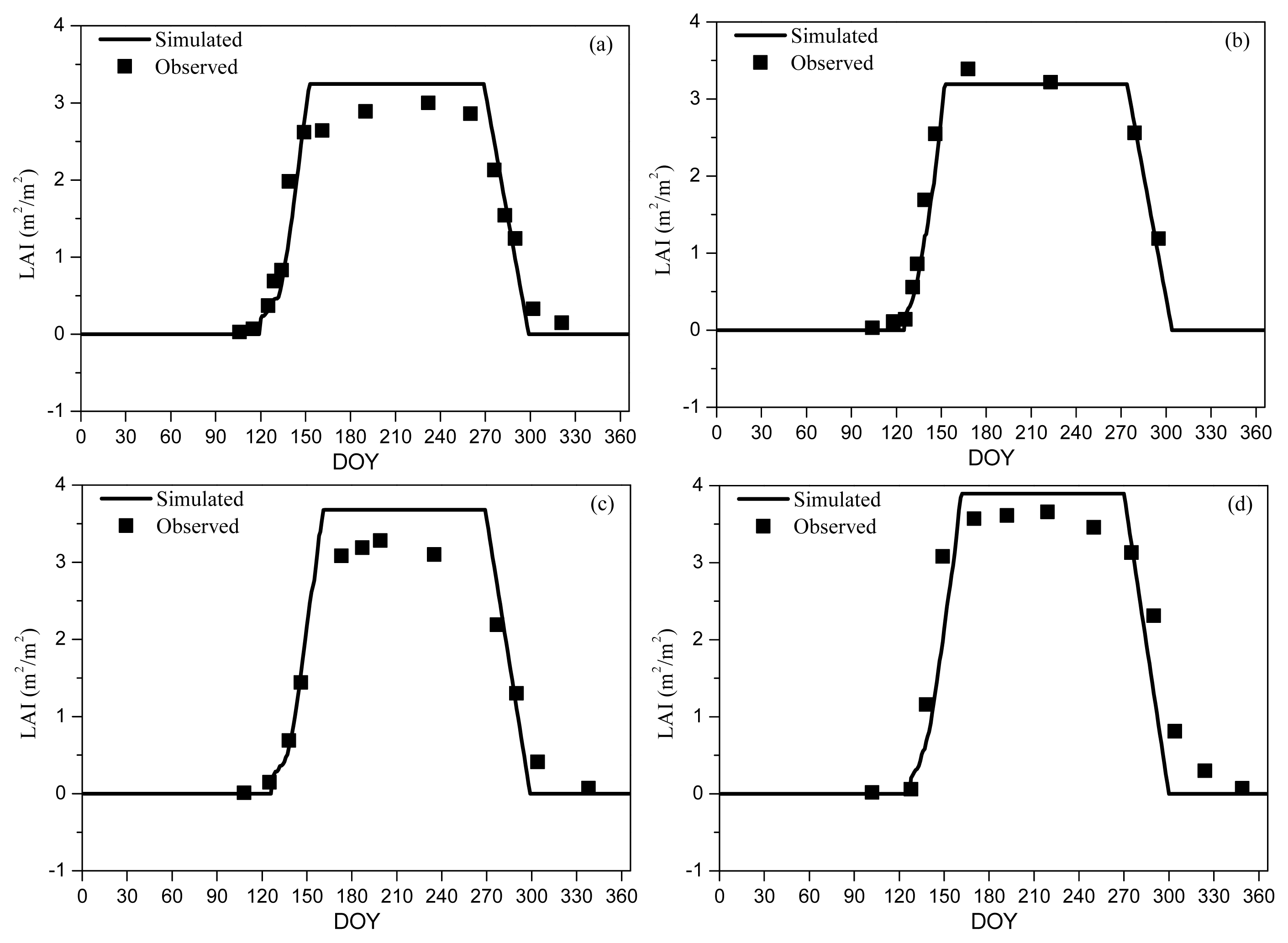
We found that Agro-IBIS had the best performance in capturing the seasonal evolution of LAI (i.e., smallest MPE between simulated and observed LAI; Table 2) with the onset prescribed as BBRK30 (i.e., the DOY when 30% of the buds have broken) and the offset prescribed as LCOLOR20 (i.e., the DOY when 20% of the leaves have changed color) (Figure 1). These two metrics represent well the beginning of the increase in LAI in spring and the decrease in autumn. Because L75 and L95 occur around the time when LAI nearly reaches its peak value, which is much later than the leaf onset defined in Agro-IBIS, they were excluded from the analysis. Although LFALL is consistent with the definition of leaf offset at first sight, our analysis suggests that even LFALL10 (close to LCOLOR80) is too late to represent the leaf offset. In spring, the simulated LAI accumulates a little slower than the observation, while the simulated LAI generally decreases faster than the observation in autumn, particularly in 2007. Our analysis shows that the model slightly overestimates the peak value of LAI.

Table 2.
Mean percentage error between simulated and observed LAI for different simulations.

Figure 1.
Simulated and observed LAI for 1998 (RMSD = 0.33) (a); 1999 (RMSD = 0.24) (b); 2006 (RMSD = 0.37) (c); and 2007 (RMSD = 0.53) (d). BBRK30 and LCOLOR20 were used in the Agro-IBIS simulation as leaf onset and offset, respectively. Observed LAI was measured using a LAI2000 sensor at Harvard Forest AmeriFlux site.
The Agro-IBIS model performed well in simulating annual GPP, Re and NEP (Figure 2). The magnitudes of these variables were reproduced well compared with the eddy covariance measurements. The multi-year average GPP, Re and NEP observations were 1428.2 g C m−2, 1135.1 g C m−2, and 293.1 g C m−2, respectively; while for the Agro-IBIS simulation, they were 1420.1 g C m−2, 1196.7 g C m−2, and 223.4 g C m−2. The model captured the inter-annual variability in GPP relatively well with a correlation of 0.5. In contrast, the correlations for Re and NEP were 0.29 and 0.18, respectively, suggesting the model did not capture the inter-annual variability in Re and NEP, particularly for the last four years of the simulation (Figure 2).
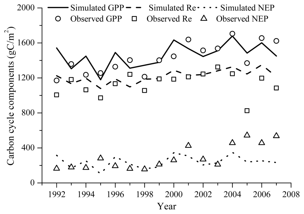
Figure 2.
Simulated and observed annual GPP (RMSD = 148.3 g C m−2), Re (RMSD = 137.3 g C m−2) and NEP (RMSD = 157.7 g C m−2). Observation is aggregated from the hourly gap-filled eddy covariance measurements. Simulated GPP was computed within the vegetation dynamics module of Agro-IBIS; Re was computed within both the vegetation dynamics module and belowground carbon cycling module of Agro-IBIS, NEP was computed as the difference between GPP and Re.
3.2. Remotely Sensed Phenological Metrics
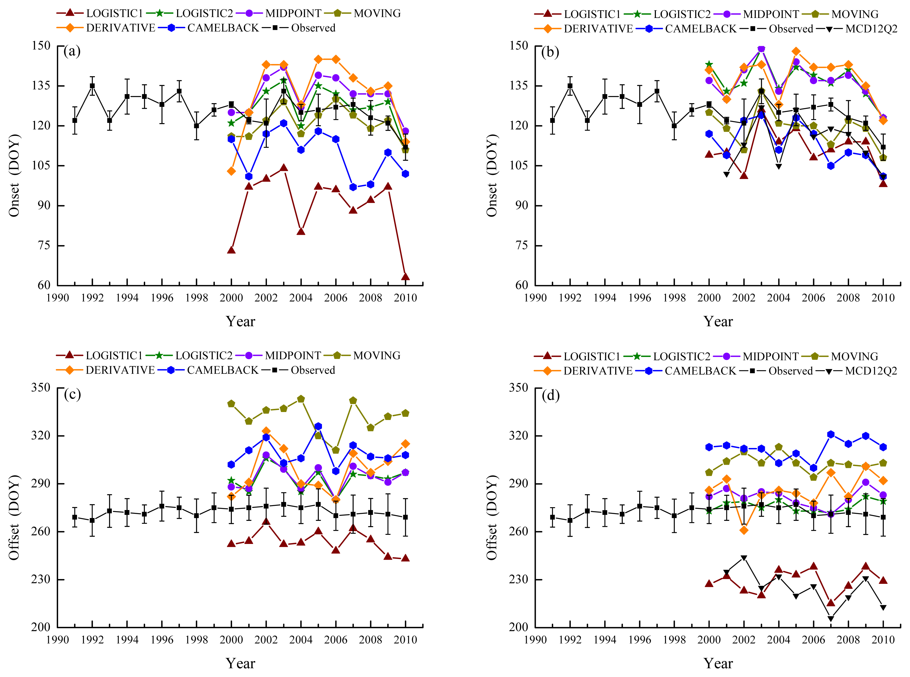
Figure 3 shows the BBRK30 and LCOLOR20 for 1991–2010 along with the remotely sensed onset and offset derived using satellite methods for 2000–2010. At Harvard Forest, BBRK30 varies in the range of DOY112 to DOY135 with an average date of DOY125. In each year, BBRK30 also varies across species and individual trees. The standard deviation fell in the range of 1.1–9.0 days. When NDVI was used to retrieve the leaf onset, LOGISTIC1 and CAMELBACK produced earlier dates than BBRK30 (Figure 3a) with an RMSD of 36.1 and 16.5 days (Table 3), respectively. The onset dates retrieved using LOGISTIC2 and MOVING varied around BBRK30 showing the smallest RMSD (less than a week) and relatively high ρ (Figure 3a, Table 3). MIDPOINT and DERIVATIVE generally produced onset dates that are later than BBRK30. MOVING had the best performance capturing the inter-annual variability with the highest ρ of 0.54 (Table 3), whereas the ρ of LOGISTIC1, CAMELBACK and DERIVATIVE were relatively low (Table 3). When EVI was used to retrieve the leaf onset, LOGISTIC1 and CAMELBACK still produced earlier dates although they were closer to BBRK30, whereas LOGISTIC2, MIDPOINT and DERIVATIVE produced later dates (Figure 3b). The RMSD of LOGISTIC2, MIDPOINT and MOVING were larger than those when NDVI was used (Table 3). For all the methods, the onset dates derived from EVI have better correlation with BBRK30 than those derived from NDVI (Table 3), suggesting that the inter-annual variability was better captured with EVI.
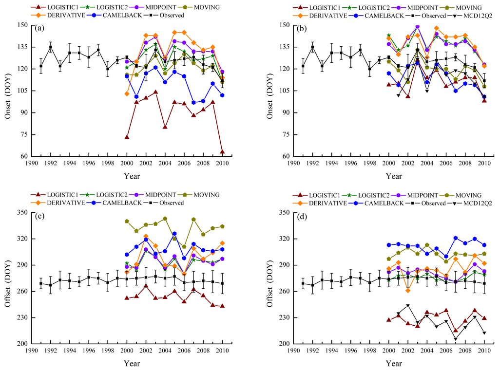
Figure 3.
Ground observed phenology with remotely sensed onset from NDVI (a); onset from EVI (b); offset from NDVI (c); and offset from EVI (d). Error bars indicate the standard deviation of observation.

Table 3.
Performance of remotely sensed onset.
The average date of LCOLOR20 at Harvard Forest is DOY273 over the period of 1991–2010 with relatively small inter-annual variability (Figure 3c). However, in a certain year, the difference between individual trees is larger than that for BBRK30 (the standard deviation ranges from 5.8–12.7 days). When NDVI was used to retrieve the offset, all the methods produced later dates than LCOLOR20 except for LOGISTIC1 (Figure 3c). The discrepancy was large with the RMSD ranging from 20.6–59.1 days (Table 4). The correlations between remotely sensed offsets and LCOLOR20 were weak (Table 4). A similar pattern was found for the offsets retrieved using EVI (Figure 3d) except that the later dates were closer to LCOLOR20 (i.e., smaller RMSD) whereas the earlier dates (i.e., offset derived using LOGISTIC1) were farther. LOGISTIC2 had relatively good performance as the offsets fell within one standard deviation of the ground observation for most years. LOGISTIC1, DERIVATIVE and CAMELBACK were negatively correlated with LCOLOR20, whereas MOVING showed relatively high ρ (Table 4). Moreover, the phenology from the MCD12Q2 product showed similar biases as LOGISTIC1 with EVI calculated using MOD09A1 (Figure 3b,d, Tables 3 and 4).

Table 4.
Performance of remotely sensed offset.
3.3. The Propagation of Bias in Phenology
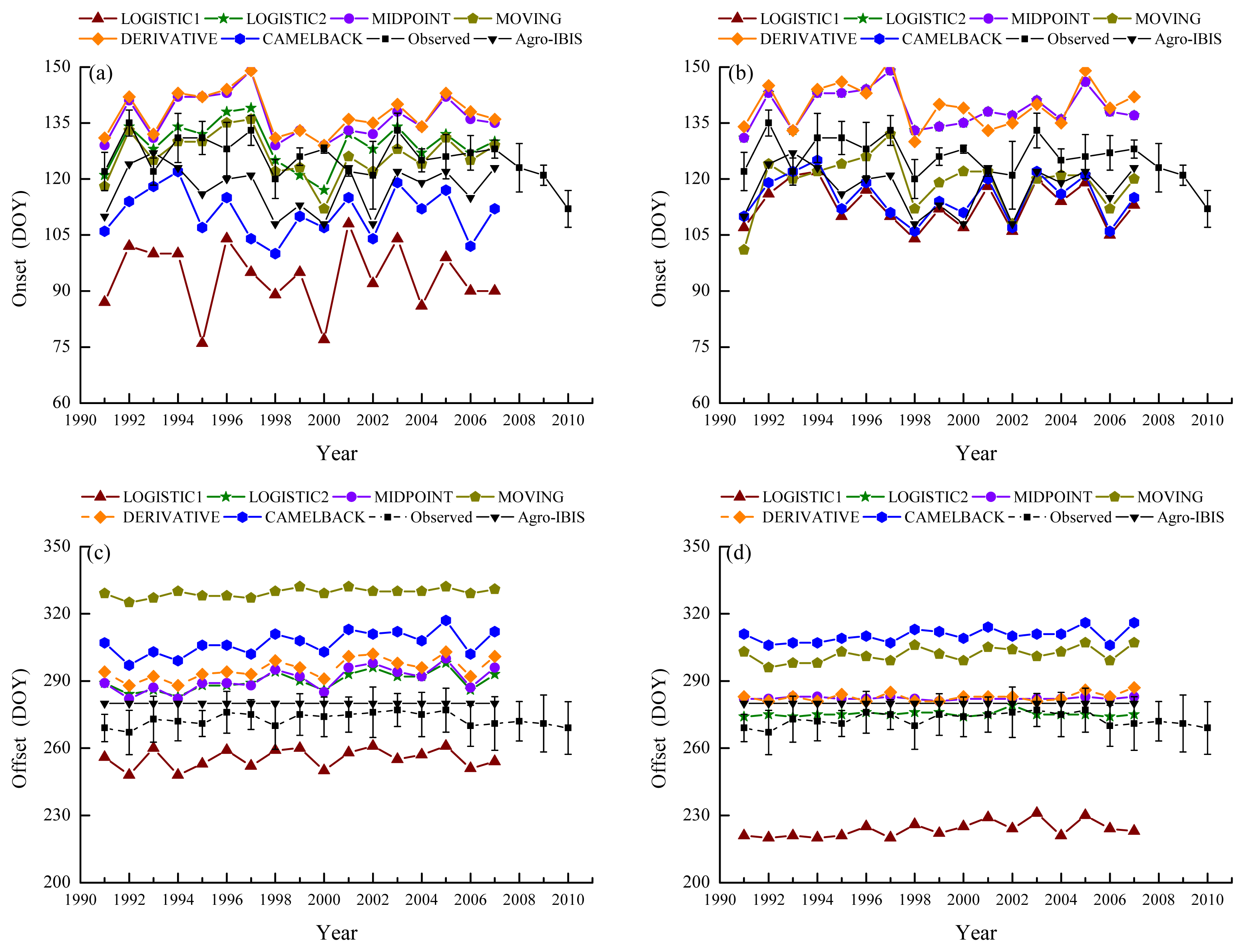
With different remotely sensed phenological metrics used as reference, the parameters of phenological models showed different capabilities of being optimized. For the “Sequential” model, the RMSD between modeled and remotely sensed onset was minimized to a range of 4.0–10.2 days. Specific RMSD depended on the combination of method and VI used to retrieve the onset. The RMSD from the “Delpierre” model ranged from 3.4–11.8 days. The modeled phenology generally showed a similar pattern of bias as the remotely sensed phenology used for parameterization in terms of whether it is earlier or later than the ground observation (Figure 4). When the onsets derived from NDVI were used as reference to parameterize the “Sequential” model, LOGISTIC1, LOGISTIC2, MOVING and DERIVATIVE showed a smaller RMSD (Table 5) than that between the remotely sensed onset and BBRK30 (Table 3), suggesting that the modeled onsets were closer to the ground observation. The correlation was increased for all the methods except CAMELBACK. When the onsets derived from EVI were used for parameterization, LOGISTIC1, LOGISTIC2, MIDPOINT and DERIVATIVE showed a slightly reduced RMSD; and LOGISTIC1, LOGISTIC1 and CAMELBACK showed a decrease in the correlation coefficient.
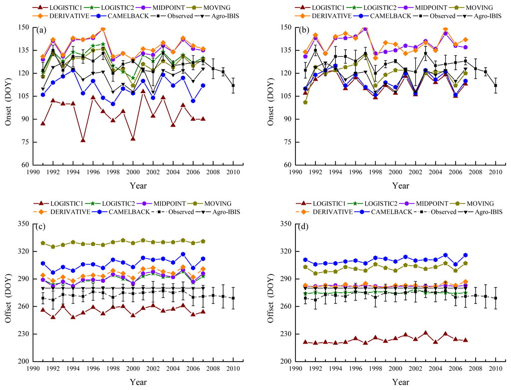
Figure 4.
Ground observed and simulated phenology. Error bars indicate the standard deviation of observation. “Agro-IBIS” is the leaf onset or offset simulated using the original Agro-IBIS algorithm and parameters. Onset was simulated using the “Sequential” model and the parameters were optimized with onset derived from NDVI (a); and EVI (b); offset was simulated using the “Delpierre” model and parameters were optimized with offset derived from NDVI (c); and EVI (d).

Table 5.
Performance of modeled onset.
The modeled leaf offsets showed smaller RMSD and higher correlation with the ground observation when the offsets derived from NDVI were used as reference to parameterize the “Delpierre” model, regardless of methods (Tables 4 and 6). In contrast, when the offsets derived from EVI were used as reference, increased RMSD was only found for LOGISTIC1. MIDPOINT and MOVING showed lower correlation coefficient, while the other methods showed higher correlation coefficient.

Table 6.
Performance of modeled offset.
Moreover, the leaf onset simulated using the Agro-IBIS algorithm was generally earlier than the ground observation (Figure 4) with an RMSD of 10.9 days. The correlation coefficient was 0.43, suggesting the inter-annual variability is not represented well. The leaf offset simulated using the Agro-IBIS algorithm was constant at DOY280 during the simulation period, which implies that the offset is only controlled by photoperiod, even though low temperature is also considered in the algorithm.
3.4. Impact of Bias in Phenology on Simulated Productivities
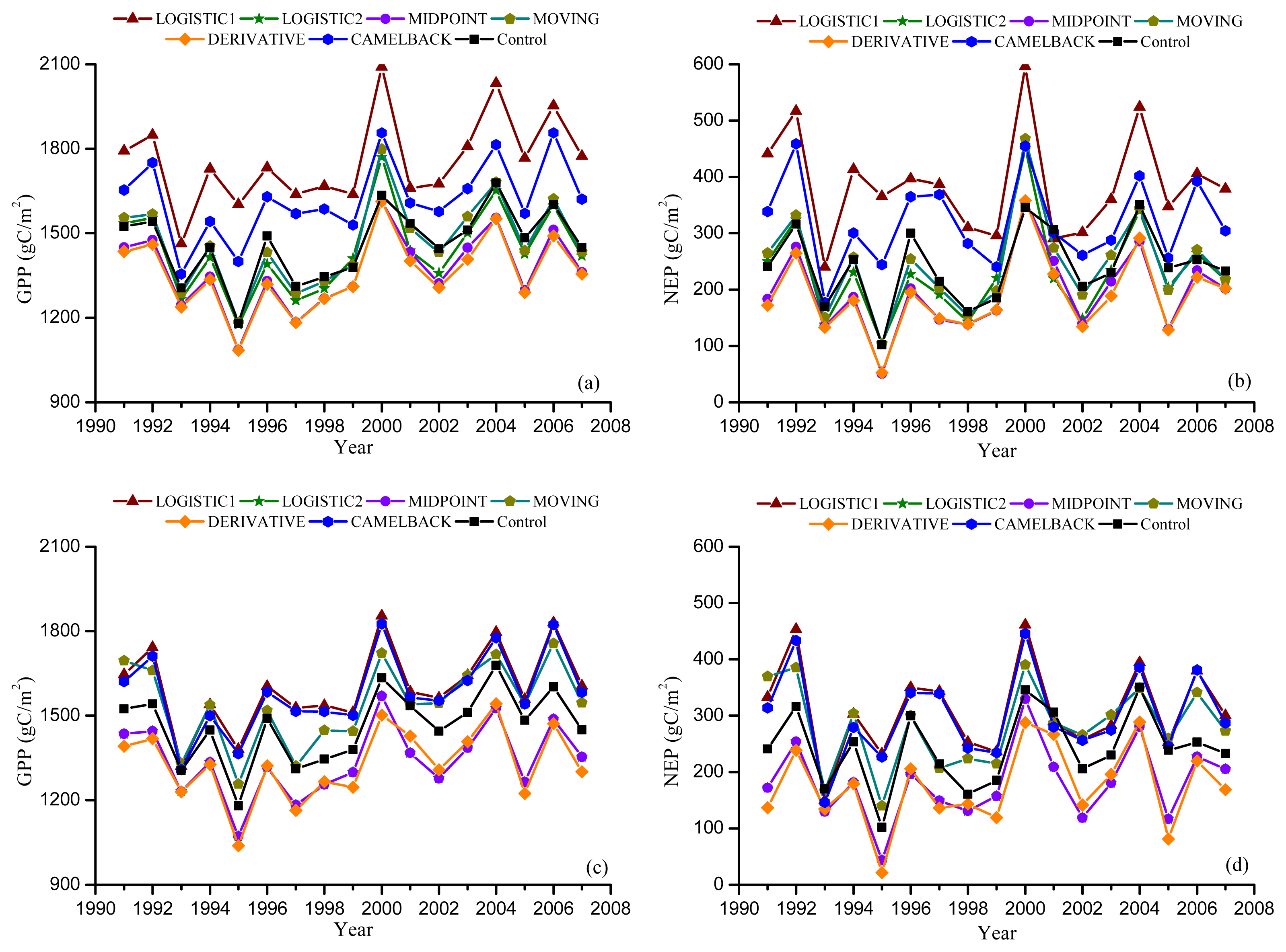
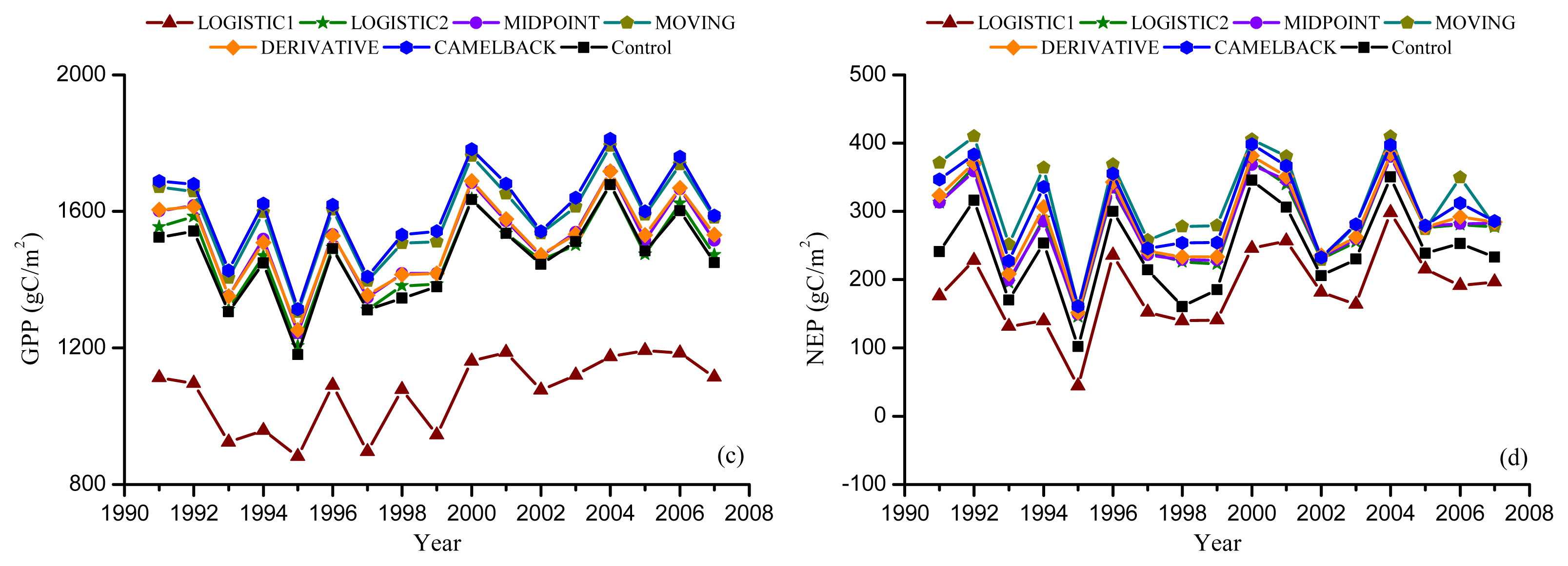
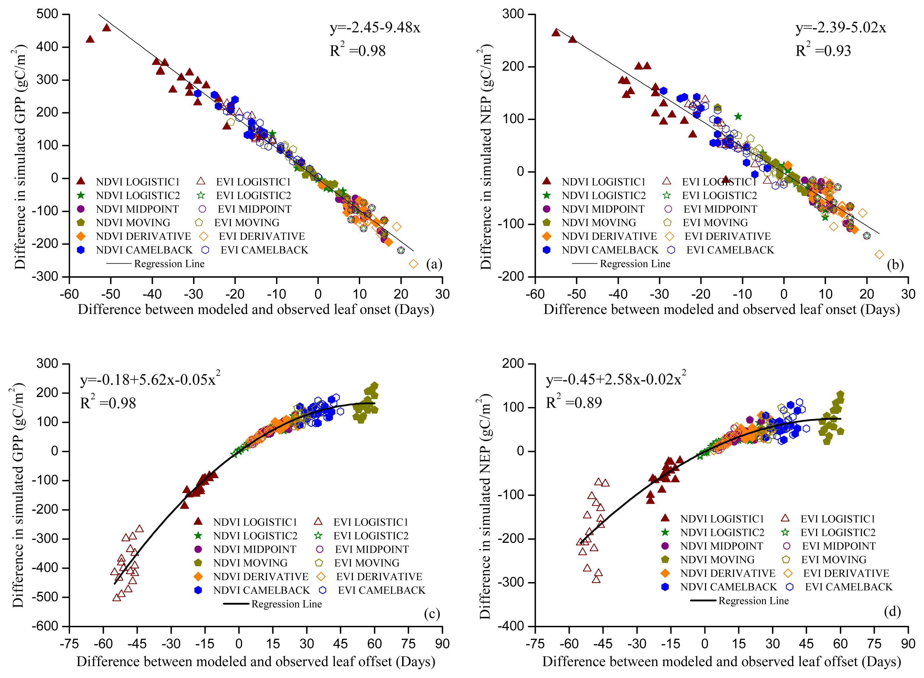
Figures 5 and 6 show the GPP and NEP simulated in the Dynamic Onset and Dynamic Offset runs, respectively. The GPP and NEP from experimental simulations have similar inter-annual variability as the control; however, their magnitude was overall increased or decreased compared with the control. This corresponds to the overall advanced or delayed phenology in the experimental simulations because the environmental conditions are the same. In general, higher GPP and NEP were found for earlier onset and later offset, mainly due to the extra days of photosynthesis. Our regression analysis showed a strong negative linear correlation between the bias in the onset (i.e., difference between modeled onset and observed onset) and the error in simulated productivities (i.e., difference in simulated GPP and NEP between the Dynamic Onset experiment and the control) (Figure 7a,b). It should be noted that, because our control simulation does not perfectly reproduce the observation (Figure 2), the difference between the experimental and control run might not perfectly represent the overall error (i.e., the difference between simulation and reality). Instead, the difference represents a component of the overall error due to inaccurate phenology, which we refer to as error in this paper for simplicity. The slopes for GPP (R2 = 0.98, p < 0.01) and NEP (R2 = 0.93, p < 0.01) were −9.48 and −5.02, respectively, indicating that a one-day bias in the leaf onset would result in an error of 9.48 g C m−2 yr−1 in GPP and 5.02 g C m−2 yr−1 in NEP. The difference in simulated GPP and NEP between the Dynamic Offset and the control can be represented as a quadratic function of the difference between modeled and observed leaf offset (Figure 7c,d). As the coefficients of the quadratic term were small (−0.05 for GPP and −0.02 for NEP), the relationship is approximately linear when the bias in offset is small (e.g., when the bias is less than 10 days). The quadratic relationship also implies that the magnitude of errors in productivities resulting from a negative bias (i.e., earlier offset) is larger than that resulting from a positive bias (i.e., later offset). Moreover, the correlation between the errors in simulated GPP and the bias in phenology is slightly stronger than that between the errors in NEP and the bias in phenology. Since NEP is the difference between GPP and Re, this implies that the Re is not as strongly controlled by the phenology as the photosynthesis.
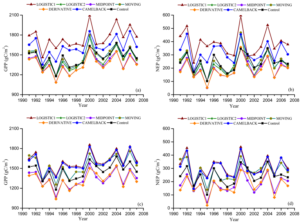
Figure 5.
Simulated annual Gross Primary Productivity (GPP) and Net Ecosystem Production (NEP) from Dynamic Onset experiment. Leaf onset dates were simulated using the “Sequential” model with the parameters optimized against remotely sensed onset using NDVI (a,b), and EVI (c,d).
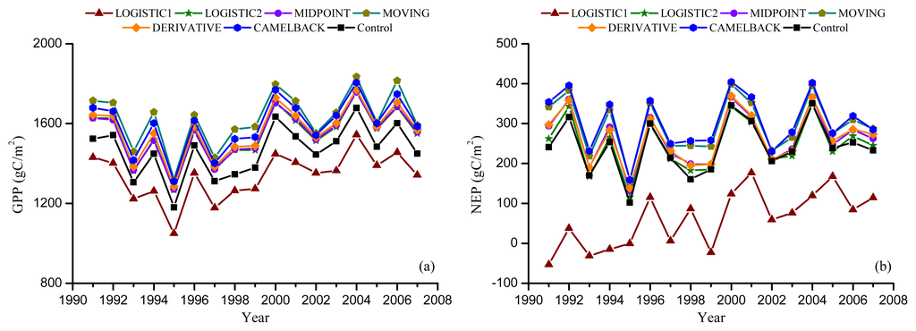
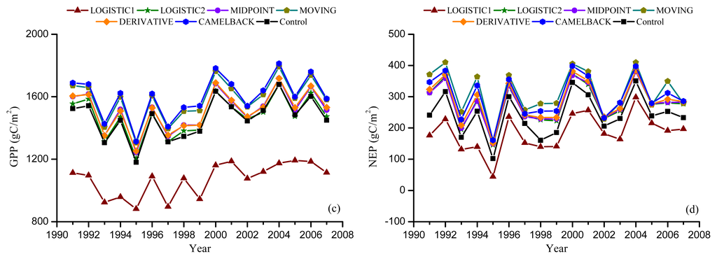
Figure 6.
Simulated annual GPP and NEP from Dynamic Offset experiment. Leaf offset dates were simulated using the “Delpierre” model with the parameters optimized against remotely sensed offset using NDVI (a,b), and EVI (c,d).
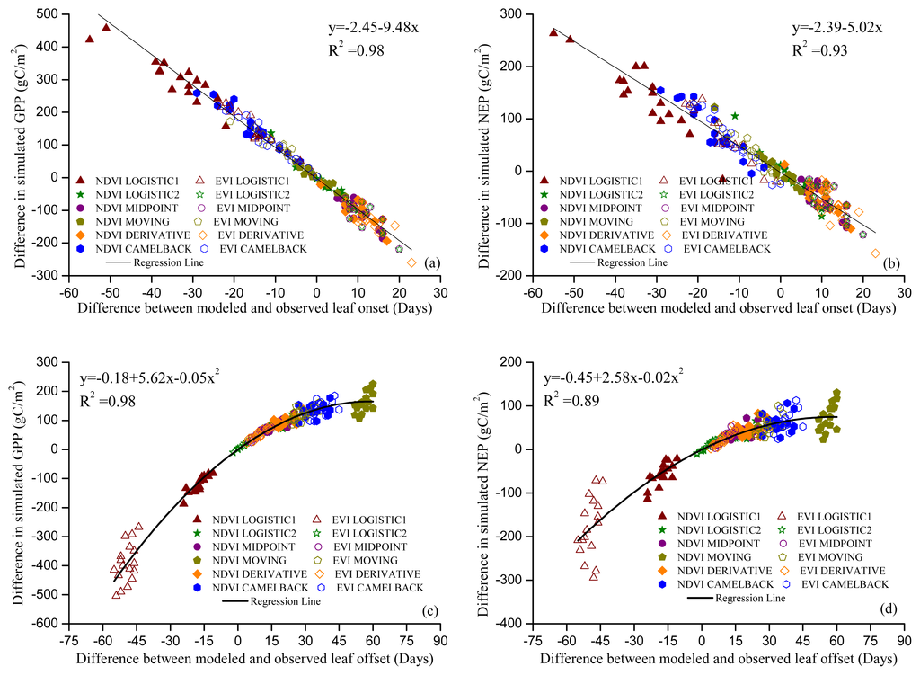
Figure 7.
Relationship between errors in phenology and errors in simulated productivities. Leaf onset vs. GPP (a); leaf onset vs. NEP (b); leaf offset vs. GPP (c) and leaf offset vs. NEP (d). Regressions were conducted using all data in the same category of simulations. P-Value for all regressions is less than 0.01. Symbols indicate the phenology method used. For example, “NDVI LOGISTIC1” in (a) indicates that the leaf onset dates were modeled using the “Sequential” model and the parameters were optimized with onset dates derived from NDVI using method “LOGISTIC1”.
4. Discussion
4.1. Ground Phenology Reference and Agro-IBIS
Our choice of ground phenology reference was based on the model performance in simulating the evolution of LAI. This method allowed us to choose the ground phenology reference quantitatively. Due to data limitation (data missing for some required variables), the model was driven with gridded climate data rather than site-specific measurements. We therefore expect some uncertainties associated with the comparison of LAI at different spatial scales (AmeriFlux site vs. simulation in a 5-min grid cell). In addition, the differences in MPE resulting from different combinations of BBRK and LCOLOR are relatively small (Table 2). This is due to the small difference between phenological levels, which were derived from interpolation. On average, it takes 4.7 days for the buds to break from 10%–90%. Therefore, in some years, the adjacent two phenological levels (e.g., BBRK20 and BBRK30) could be the same. As it takes longer for the leaves to change color (e.g., 9.5 days on average from 10%–50% coloring), the difference resulting from different LCOLOR levels is larger (Table 2). Although uncertainties remain in the chosen ground phenology reference, they were confined to a small range based on our choice of metrics. The uncertainties in the offset are larger than those in the onset due to the larger variability in the offset across species and individual trees.
Agro-IBIS captured the magnitude of productivity variables when compared with observations, although uncertainties exist because of model limitations. For example, the slower increase in LAI in spring compared with the observations (Figure 1) results from a small underestimation in net primary productivity (NPP), a component of simulated LAI. The faster decrease in simulated LAI in autumn might be because of the relatively simple scheme used in Agro-IBIS. Once the offset is triggered, the LAI decreases linearly to a minimum over a 30-day period. However, as the canopy photosynthesis is scaled using LAI in the model, the faster decrease in LAI can partly correct the errors caused by not taking into account the effect of leaf age and coloring.
The discrepancies between the simulated carbon cycle components and the flux measurements can be explained by the following possible reasons: (1) the grid cell was simulated as temperate deciduous forest so that only one PFT existed [34]; (2) the footprints of other PFTs such as evergreen trees and understory shrubs were not simulated although they are likely small; (3) the meteorological data used to drive the model represents the average condition of a grid cell, which could be slightly different from the real condition at the site; and (4) there might also be uncertainties in the flux measurements and the post-processing such as gap-filling [48].
4.2. Remotely Sensed Phenology
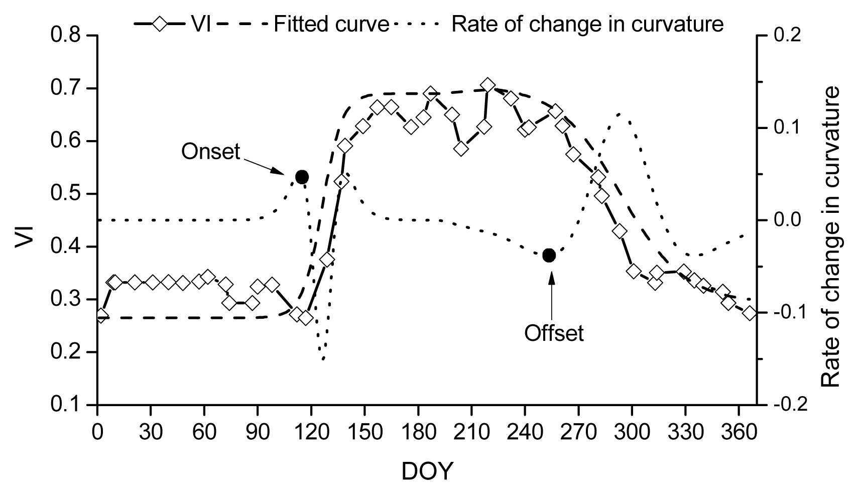
With the remote sensing product chosen in this study, including the products shown in the supplementary material, most of the six remote sensing methods in this study show relatively poor performance compared with the ground-observed phenology, regardless of which VI is used. The discrepancy can be explained by several possible reasons, within which the difference in definition perhaps having the largest contribution. For example, the onset retrieved using DERIVATIVE is later than BBRK30 (Figure 3a) because the maximum of the first derivative of VI time series represents the time when VI increases the fastest, which usually responds to the period of fast leaf expansion after all buds have broken. LOGISTIC2 and MIDPOINT arbitrarily define the onset as the time when 50% of the amplitude between the minimum and maximum of either fitted or normalized VI time series is reached, which is expected to be later than the time when buds break. LOGISTIC1 and CAMELBACK are both based on the second derivative of VI time series. The local maximum of the second derivative tends to capture the subtle change in the VI, which is too sensitive to the growth of understory that occurs earlier than the development of canopy [22,49]. The onset retrieved using LOGISTIC1 can also be affected by the curve fitting, because the maximum rate of change in the curvature is determined by the shape of the fitted curve (i.e., the parameters of logistic function), and the shape is controlled by how the VI changes when it starts increasing as well as when it reaches the peak.
For the offset, MOVING and CAMELBACK use a process symmetrical to the onset. Because the onset derived using these methods well represents the period when LAI starts to increase from the minimum value, the offset tends to represent the period when LAI drops to the minimum value, which is much later than when LCOLOR20 is reached. LOGISTIC2, MIDPOINT and DERIVATIVE also produce dates later than LCOLOR20 as they tend to capture the period when VI drops the fastest, which usually corresponds to the fast change in leaf color and decrease in LAI rather than the beginning of offset. Although LOGISTIC1 is trying to capture the period when VI starts to decrease, there is still a difference between the offset derived using LOGISTIC1 and that based on ground observation, because the VI does not change synchronously with LAI. Moreover, similar to the onset, the offset derived using LOGISTIC1 can be affected by the shape of the fitted curve, which is controlled by the change in VI around the period when VI drops to the minimum. Regardless of remote sensing method, offset is later when using NDVI than with EVI. This is likely because NDVI tends to saturate when the LAI is high (3 or more for a pure forest pixel) [50,51] so that it is not as sensitive as EVI to the drop in LAI. Generally, EVI is more responsive to the canopy structural variation, such as LAI, and NDVI is more sensitive to chlorophyll [52].
There is a difference between the phenological dates retrieved using LOGISTIC1 with EVI, and those from MCD12Q2, which was produced using LOGISTIC1 as well with NBAR EVI. This highlights the fact that the phenology retrieved can also be affected by factors other than the method, such as the choice of data source (see Supplementary Material) [28] and data processing. On the other hand, the similar patterns shown by the two results suggest that the general features of a certain method are relatively independent of data source. Another issue related to the satellite methods is the parameterization. The width of the moving window used in MOVING, DERIVATIVE and CAMELBACK as well as the 50% amplitude used in LOGISTIC2 and MIDPOINT can be considered as parameters. Because those parameters were chosen based on the input data used when developing the method, when the data source changes, they may no longer be optimal and can contribute to the discrepancies between the remotely sensed phenology and the ground observation. Our preliminary investigation suggests that, by adjusting parameters, it is possible to reduce the discrepancy between remotely sensed phenology and the ground phenology reference at a specific site (see Figure S3 in Supplementary Material). However, these parameters must be evaluated at other locations. Currently, long-term ground observations of phenology are limited, and the phenology is usually recorded in different ways at different locations (e.g., Harvard Forest vs. Hubbard Brook Experimental Forest), which causes evaluation to be confounded [53]. Recently, digital cameras have been widely installed to observe vegetation phenology. Since the phenological information gathered from digital camera can be standardized, it can potentially be used to validate the phenology retrieved from satellite imagery at multiple locations, and help resolve the issue of scale difference between ground observations and satellite imagery (i.e., individual trees vs. pixels) [54].
4.3. Modeled Phenology
Differences in RMSD and correlation coefficient between the modeled and observed phenology have been found in comparison with those between the corresponding remotely sensed phenology and ground observation. However, there is no evident pattern of whether the RMSD and correlation coefficient would increase or decrease, which suggests that the discrepancy between modeled and remotely sensed phenology may either add to or offset the discrepancy between remotely sensed phenology and ground observations. Overall, the magnitude of differences in the RMSD is small (usually less than 1 day for the onset, and less than 5 days for the offset). Thus, the RMSD between modeled and observed phenology is still on the same order as the RMSD between the phenology used for parameterization and observed on the ground. In other words, the bias in remotely sensed phenology is generally maintained by the modeled phenology. The magnitude of changes in correlation varies in a relatively wide range (Table 3 vs. Table 5 and Table 4 vs. Table 6), because the correlation is not considered in the cost function of the genetic algorithm. In most cases, correlation became lower suggesting the capability of capturing the inter-annual variability is weakened after the modeling process. Even though correlation became higher in some cases, it does not necessarily indicate that the capability of capturing the inter-annual variability has been improved. If the modeling period were extended, the correlation might further change. This highlights the fact that there is still a need to evaluate whether the phenological models and the optimized parameters can properly capture the changes in phenology in response to the changing climate, even if the RMSD is minimized. One possible solution is to maximize the correlation between modeled phenology and the reference and minimize the RMSD during the optimization process, which requires developing a cost function that incorporates both metrics.
4.4. Impact of Phenology on Simulated Productivities
Our analysis indicates that errors in simulated GPP and NEP result from the bias in simulated phenology (Figures 5 and 6). Although the sign of NEP did not change due to the bias in phenology, as the study site is a relatively large carbon sink, this might not be the case at other locations that are closer to carbon neutral. The relationship between the errors in simulated GPP and NEP and the bias in phenology also has implications on the impact of phenological shifts on carbon assimilation. The linear relationship between errors in GPP and NEP and the bias in leaf onset means that a one-day advance in leaf onset would result in an increase of 9.48 g C m−2 yr−1 in GPP and 5.02 g C m−2 yr−1 in NEP (Figure 7a,b). The quadratic relationship between errors in GPP and NEP and the bias in leaf offset (Figure 7a,b) suggests that delayed leaf offset leads to higher GPP and NEP. However, the marginal increase in GPP and NEP declines with the days of delay. This might be because the environmental condition becomes less and less favorable for carbon uptake late in a year.
Because growing season length (GSL) is determined by leaf onset and offset, productivity is usually correlated with GSL. Previous studies have shown significant control of GSL on the productivities. For example, a modeling study found that an extension of one day in GSL would result in an increase of 9.8 ± 2.6 g C m−2 yr−1 in GPP for temperate deciduous broadleaf forest [55]; carbon flux measurements showed an increase of 5.57 m−2 yr−1 in NEP with a one-day extension of carbon uptake period (i.e., number of days when it is a net carbon sink), which is an alternative definition of GSL [56]. These relationships are similar to the impact of leaf onset on the productivities estimated from our simulations. This might be explained by the fact that the variation in GSL in those studies was dominated by the variation in leaf onset [55]. On the other hand, although our analysis indicates that the productivities are less sensitive to leaf offset than to leaf onset in Agro-IBIS, further analysis with measurements is still needed to evaluate to what extent these sensitivities represent reality. For example, a study using different phenological indicators suggested that the productivities are more sensitive to autumn senescence [57]. Despite the discrepancy, our analysis suggests that it might be better to examine the individual impact of leaf onset and offset instead of the overall impact of GSL.
4.5. Uncertainties in the Evaluation
There are several factors that have influenced our evaluation and contributed to the associated uncertainties. First, our evaluation is limited to Harvard Forest due to data availability; therefore, the results may not be representative for other locations with different species composition. Second, the uncertainties in ground observations, including phenology (e.g., large variation in observed leaf offset, Figure 3), LAI and carbon flux could propagate into our evaluation. Third, as simulated LAI was compared with site-level observation, the limitation of the Agro-IBIS model (e.g., linear decrease of LAI in a fixed period in autumn) and different spatial scales (grid cell vs. site) might introduce uncertainties in the selection of ground phenology reference. Finally, different data processing strategies (e.g., smoothing and interpolation of vegetation indices) might cause differences in the phenology derived using the same methods. In order to reduce such uncertainties, comprehensive evaluation at different locations should be conducted with ground phenological observations that can be standardized and that have a spatial scale more consistent with the satellite (e.g., images from “PhenoCam” [54]).
5. Conclusions
We used long-term ground phenological observations along with leaf area index and carbon flux measurements made at Harvard Forest to evaluate six vegetation-index-based methods for retrieving phenology. Our analysis shows that, compared with the ground phenology reference chosen according to the definition in the Agro-IBIS dynamic ecosystem model, phenology derived using the evaluated methods generally had relatively large discrepancies, which could be attributed to the different definitions of phenology, the parameters used for a certain method, and the input data. However, two methods for leaf onset (i.e., LOGISTIC2 [22] and MOVING [23]) and one method for leaf offset (i.e., LOGISTIC2 [22]) showed a bias of less than a week, and could be further improved, suggesting that phenological metrics derived using these methods could potentially be used in dynamic ecosystem models similar to Agro-IBIS. Our analysis shows that, when remotely sensed phenological metrics are used to parameterize phenological models, the bias is generally maintained in the modeled phenology, and will propagate to cause errors in productivities simulated in dynamic ecosystem models. The different sensitivities of Agro-IBIS to leaf onset and offset suggest that the impact of spring and autumn phenology on carbon assimilation should be examined separately. Our evaluation was conducted at one site due to data availability, and subject to uncertainties associated with ground observations, model simulations, and data processing. However, the evaluation procedure proposed in this study, including quantitative selection of ground reference, comparison between multiple data sources and examination of bias propagation, can provide guidance for further evaluation at more locations.
Supplementary Information
remotesensing-06-04660-s001.pdfAcknowledgments
We thank three anonymous reviewers for their constructive comments and suggestions, which helped to improve our manuscript.
Conflicts of Interest
The authors declare no conflict of interest.
- Author ContributionsHong Xu and Tracy E. Twine designed the research. Hong Xu and Xi Yang performed data analysis and model simulations. All authors contributed with ideas, writing and discussions.
References
- Menzel, A.; Fabian, P. Growing season extended in Europe. Nature 1999, 397, 659. [Google Scholar]
- Myneni, R.B.; Keeling, C.D.; Tucker, C.J.; Asrar, G.; Nemani, R.R. Increased plant growth in the northern hight latitudes from 1981 to 1991. Nature 1997, 386, 698–702. [Google Scholar]
- Schwartz, M.D.; Reiter, B.E. Changes in north American spring. Int. J. Climatol 2000, 20, 929–932. [Google Scholar]
- Zhou, L.; Tucker, C.J.; Kaufmann, R.K.; Slayback, D.; Shabanov, N.V.; Myneni, R.B. Variation in northern vegetation activity inferred from satellite data of vegetation index during 1981 to 1999. J. Geophys. Res 2001, 106, 20069–20083. [Google Scholar]
- Zhu, W.; Tian, H.; Xu, X.; Pan, Y.; Chen, G.; Lin, W. Extension of the growing season due to delayed autumn over mid and high latitudes in north America during 1982–2006. Glob. Ecol. Biogeogr 2012, 21, 260–271. [Google Scholar]
- Menzel, A.; Sparks, T.H.; Estrella, N.; Koch, E.; Aasa, A.; Ahas, R.; Alm-Kubler, K.; Bissolli, P.; Braslavska, O.G.; Briede, A.; et al. European phenological response to climate change matches the warming pattern. Glob. Chang. Biol 2006, 12, 1969–1976. [Google Scholar]
- Peñuelas, J.; Filella, I. Phenology-responses to a warming world. Science 2001, 294, 793–795. [Google Scholar]
- Peñuelas, J.; Rutishauser, T.; Filella, I. Phenology feedbacks on climate change. Science 2009, 324, 887–888. [Google Scholar]
- Richardson, A.D.; Keenan, T.F.; Migliavacca, M.; Ryu, Y.; Sonnentag, O.; Toomey, M. Climate change, phenology, and phenological control of vegetation feedbacks to the climate system. Agric. For. Meteorol 2013, 169, 156–173. [Google Scholar]
- Richardson, A.D.; Anderson, R.S.; Arain, M.A.; Barr, A.G.; Bohrer, G.; Chen, G.; Chen, J.M.; Ciais, P.; Davis, K.J.; Desai, A.R.; et al. Terrestrial biosphere models need better representation of vegetation phenology: Results from the north American carbon program site synthesis. Glob. Chang. Biol 2012, 18, 566–584. [Google Scholar]
- Levis, S.; Bonan, G.B. Simulating springtime temperature patterns in the community atmosphere model coupled to the community land model using prognostic leaf area. J. Clim 2004, 17, 4531–4540. [Google Scholar]
- Migliavacca, M.; Sonnentag, O.; Keenan, T.F.; Cescatti, A.; O’Keefe, J.; Richardson, A.D. On the uncertainty of phenological responses to climate change, and implications for a terrestrial biosphere model. Biogeosciences 2012, 9, 2063–2083. [Google Scholar]
- Yang, X.; Mustard, J.F.; Tang, J.; Xu, H. Regional-scale phenology modeling based on meteorological records and remote sensing observations. J. Geophys. Res 2012, 117, G03029. [Google Scholar]
- Fisher, J.I.; Richardson, A.D.; Mustard, J.F. Phenology model from surface meteorology does not capture satellite-based greenup estimations. Glob. Chang. Biol 2007, 13, 707–721. [Google Scholar]
- De Beurs, K.M.; Henebry, G.M. Land surface phenology and temperature variation in the international geosphere-biosphere program high-latitude transects. Glob. Chang. Biol 2005, 11, 779–790. [Google Scholar]
- Liang, L.; Schwartz, M.D. Landscape phenology: An integrative approach to seasonal vegetation dynamics. Landsc. Ecol 2009, 24, 465–472. [Google Scholar]
- Zhang, X.; Tarpley, D.; Sullivan, J.T. Diverse responses of vegetation phenology to a warming climate. Geophys. Res. Lett 2007, 34, L19405. [Google Scholar]
- Botta, A.; Viovy, N.; Ciais, P.; Friedlingstein, P.; Monfray, P. A global prognostic scheme of leaf onset using satellite data. Glob. Chang. Biol 2000, 6, 7090–7725. [Google Scholar]
- White, M.A.; Thornton, P.E.; Running, S.W. A continental phenology model for monitoring vegetation responses to interannual climatic variability. Glob. Biogeochem. Cycles 1997, 11, 217–234. [Google Scholar]
- Balzter, H.; Gerard, F.; George, C.; Weedon, G.; Grey, W.; Combal, B.; Bartholomé, E.; Bartalev, S.; Los, S. Coupling of vegetation growing season anomalies and fire activity with hemispheric and regional-scale climate patterns in central and east Siberia. J. Clim 2007, 20, 3713–3729. [Google Scholar]
- De Beurs, K.M.; Henebry, G.M. Northern annular mode effects on the land surface phenologies of northern Eurasia. J. Clim 2008, 21, 4257–4279. [Google Scholar]
- Fisher, J.I.; Mustard, J.F.; Vadeboncoeur, M.A. Green leaf phenology at landsat resolution: Scaling from the field to the satellite. Remote Sens. Environ 2006, 100, 265–279. [Google Scholar]
- Reed, B.C.; Brown, J.F.; Vanderzee, D.; Loveland, T.R.; Merchant, J.W.; Ohlen, D.O. Measuring phenological variability from satellite imagery. J. Veg. Sci 1994, 15, 703–714. [Google Scholar]
- Tateishi, R.; Ebata, M. Analysis of phenological change patterns using 1982–2000 advanced very high resolution radiometer (AVHRR) data. Int. J. Remote Sens 2004, 25, 2287–2300. [Google Scholar]
- Zhang, X.; Friedl, M.A.; Schaaf, C.B.; Strahler, A.H.; Hodges, J.C.F.; Gao, F.; Reed, B.C.; Huete, A. Monitoring vegetation phenology using MODIS. Remote Sens. Environ 2003, 84, 471–475. [Google Scholar]
- Schwartz, M.D.; Reed, B.C.; White, M.A. Assessing satellite-derived start-of-season measures in the conterminous USA. Int. J. Climatol 2002, 22, 1793–1805. [Google Scholar]
- White, M.A.; de Beurs, K.M.; Didan, K.; Inouye, D.W.; Richardson, A.D.; Jensen, O.P.; O’Keefe, J.; Zhang, G.; Nemani, R.R.; van LEEUWEN, W.J.D.; et al. Intercomparison, interpretation, and assessment of spring phenology in north America estimated from remote sensing for 1982–2006. Glob. Chang. Biol 2009, 15, 2335–2359. [Google Scholar]
- Ahl, D.E.; Gower, S.T.; Burrows, S.N.; Shabanov, N.V.; Myneni, R.B.; Knyazikhin, Y.; Douglas, E.A. Monitoring spring canopy phenology of a deciduous broadleaf forest using MODIS. Remote Sens. Environ 2006, 104, 88–95. [Google Scholar]
- Foley, J.A.; Prentice, I.C.; Ramankutty, N.; Levis, S.; Pollard, D.; Sitch, S.; Haxeltine, A. An integrated biosphere model of land surface processes, terrestrial carbon balance, and vegetation dynamics. Glob. Biogeochem. Cycle 1996, 10, 603–628. [Google Scholar]
- Kucharik, C.J. Evaluation of a process-based agro-ecosystem model (Agro-IBIS) across the U.S. Corn belt: Simulations of the interannual variability in maize yield. Earth Interact 2003, 7, 1–33. [Google Scholar]
- Kucharik, C.J.; Foley, J.A.; Christine, D.; Fisher, V.A.; Coe, M.T.; Lenters, J.D.; Young-Molling, C.; Ramankutty, N.; Norman, J.M.; Gower, S.T. Testing the performance of a dynamic global ecosystem model: Water balance, carbon balance, and vegetation structure. Glob. Biogeochem. Cycle 2000, 14, 795–825. [Google Scholar]
- O’Keefe, J. Harvard Forest Data Archive: Hf003. Available online: http://harvardforest.fas.harvard.edu:8080/exist/xquery/data.xq?id=hf003 (accessed on 26 March 2014).
- Munger, J.W. Ameriflux: Harvard Forest. Available online: http://ameriflux.ornl.gov/fullsiteinfo.php?sid=50 (accessed on 26 March 2014).
- Kucharik, C.J.; Barford, C.C.; El Maayar, M.; Wofsy, S.C.; Monson, R.K.; Baldocchi, D.D. A multiyear evaluation of a dynamic global vegetation model at three ameriflux forest sites: Vegetation structure, phenology, soil temperature, and CO2 and H2O vapor exchange. Ecol. Modell 2006, 196, 1–31. [Google Scholar]
- Twine, T.E.; Kucharik, C.J. Evaluating a terrestrial ecosystem model with satellite information of greenness. J. Geophys. Res.-Biogeosci 2008, 113, G03027. [Google Scholar]
- Twine, T.E.; Kucharik, C.J. Climate impacts on net primary productivity trends in natural and managed ecosystems of the central and eastern United States. Agric. For. Meteorol 2009, 149, 2143–2161. [Google Scholar]
- Anderson-Teixeira, K.J.; Snyder, P.K.; Twine, T.E.; Cuadra, S.V.; Costa, M.H.; DeLucia, E.H. Climate-regulation services of natural and agricultural ecoregions of the Americas. Nat. Clim. Chang 2012, 2, 177–181. [Google Scholar]
- Motew, M.M.; Kucharik, C.J. Climate-induced changes in biome distribution, NPP, and hydrology in the upper midwest U.S.: A case study for potential vegetation. J. Geophys. Res.: Biogeosci 2013, 118, 248–264. [Google Scholar]
- Urbanski, S.; Barford, C.; Wofsy, S.; Kucharik, C.; Pyle, E.; Budney, J.; McKain, K.; Fitzjarrald, D.; Czikowsky, M.; Munger, J.W. Factors controlling CO2 exchange on timescales from hourly to decadal at harvard forest. J. Geophys. Res 2007, 112, G02020. [Google Scholar]
- The USGS Land Processes Distributed Active Archive Center. Available online: https://lpdaac.usgs.gov/ (accessed on 26 March 2014).
- Chen, J.; Jönsson, P.; Tamura, M.; Gu, Z.; Matsushita, B.; Eklundh, L. A simple method for reconstructing a high-quality NDVI time-series data set based on the Savitzky–Golay filter. Remote Sens. Environ 2004, 91, 332–344. [Google Scholar]
- Sarvas, R. Investigations on the annual cycle of development of forest trees: II. Autumn dormancy and winter dormancy. Commun. Instit. Forestalis Fenniae 1974, 84, 1–101. [Google Scholar]
- Delpierre, N.; Dufrene, E.; Soudani, K.; Ulrich, E.; Cecchini, S.; Boe, J.; Francois, C. Modelling interannual and spatial variability of leaf senescence for three deciduous tree species in France. Agric. For. Meteorol 2009, 149, 848–938. [Google Scholar]
- Hunter, A.F.; Lechowicz, M.J. Predicting the timing of budburst in temperate trees. J. Appl. Ecol 1992, 29, 597–604. [Google Scholar]
- Kramer, K. Selecting a model to predict the onset of growth of Fagus sylvatica. J. Appl. Ecol 1994, 31, 172–181. [Google Scholar]
- Campbell, G.S.; Norman, J.M. An Introduction to Environmental Biophysics; Springer: New York, NY, USA, 1998. [Google Scholar]
- Rob Dimeo’s IDL Programs. Available online: http://www.ncnr.nist.gov/staff/dimeo/idl_programs.html (accessed on 26 March 2014).
- Moffat, A.M.; Papale, D.; Reichstein, M.; Hollinger, D.Y.; Richardson, A.D.; Barr, A.G.; Beckstein, C.; Braswell, B.H.; Churkina, G.; Desai, A.R.; et al. Comprehensive comparison of gap-filling techniques for eddy covariance net carbon fluxes. Agric. For. Meteorol 2007, 147, 209–232. [Google Scholar]
- Richardson, A.D.; O’Keefe, J. Phenological Differences between Understory and Overstory: A Case Study Using the Long-Term Harvard Forest Records. In Phenology of Ecosystem Processes: Applications in Global Change Research; Noormets, A., Ed.; Springer: New York, NY, USA, 2009; pp. 87–117. [Google Scholar]
- Birky, A.K. NDVI a simple model of deciduous forest seasonal dynamics. Ecol. Modell 2001, 143, 43–58. [Google Scholar]
- Lüdeke, M.; Janecek, A.; Kohlmaier, G.H. Modelling the seasonal CO2 uptake by land vegetation using the global vegetation index. Tellus 1991, 43B, 188–196. [Google Scholar]
- Huete, A.; Didan, K.; Miura, T.; Rodriguez, E.P.; Gao, X.; Ferreira, L.G. Overview of the radiometric and biophysical performance of the MODIS vegetation indices. Remote Sens. Environ 2002, 83, 195–213. [Google Scholar]
- Richardson, A.D.; Bailey, A.S.; Denny, E.G.; Martin, C.W.; O’Keefe, J. Phenology of a northern hardwood forest canopy. Glob. Chang. Biol 2006, 12, 1174–1188. [Google Scholar]
- Sonnentag, O.; Hufkens, K.; Teshera-Sterne, C.; Young, A.M.; Friedl, M.; Braswell, B.H.; Milliman, T.; O’Keefe, J.; Richardson, A.D. Digital repeat photography for phenological research in forest ecosystems. Agric. For. Meteorol 2012, 152, 159–177. [Google Scholar]
- Piao, S.; Friedlingstein, P.; Ciais, P.; Viovy, N.; Demarty, J. Growing season extension and its impact on terrestrial carbon cycle in the northern hemisphere over the past 2 decades. Glob. Biogeochem. Cycle 2007, 21, GB3018. [Google Scholar]
- Baldocchi, D. Turner review No. 15. ‘Breathing’ of the terrestrial biosphere: Lessons learned from a global network of carbon dioxide flux measurement systems. Austr. J. Bot 2008, 56, 1–26. [Google Scholar]
- Richardson, A.D.; Black, T.A.; Ciais, P.; Delbart, N.; Friedl, M.A.; Gobron, N.; Hollinger, D.Y.; Kutsch, W.L.; Longdoz, B.; Luyssaert, S.; et al. Influence of spring and autumn phenological transitions on forest ecosystem productivity. Philos. Transc. R. Soc. B 2010, 365, 3227–3246. [Google Scholar]
© 2014 by the authors; licensee MDPI, Basel, Switzerland This article is an open access article distributed under the terms and conditions of the Creative Commons Attribution license (http://creativecommons.org/licenses/by/3.0/).

