1. Introduction
Light detection and ranging (LiDAR) is a laser-based, active remote sensing system, which collects ranging data utilizing the speed of light and information about the flight time of a laser pulse [
1]. In this context, flight time refers to the time it takes for a given laser pulse to travel from a system, backscatter from an object, and return back to the system. A wide variety of LiDAR systems currently exist, and data have been successfully collected utilizing systems mounted to space-borne, aerial, and terrestrial (tripod or vehicle-based) platforms.
Over the past several decades the use of LiDAR remote sensing data in forestry has seen steady growth. The increased use of LiDAR systems to acquire data over forested areas can be attributed to their ability to cover extents of local or regional scales and accurately quantify the three-dimensional structure of the forest. Previous studies have demonstrated the usefulness of LiDAR for: (1) Forest measurements [
2,
3,
4,
5,
6,
7,
8,
9,
10,
11]; (2) habitat analysis [
12,
13,
14]; (3) estimation of forest biophysical parameters [
15,
16,
17,
18,
19,
20,
21,
22,
23,
24,
25,
26,
27]; (4) change detection [
23,
28,
29]; and (5) estimation of wild land fire parameters [
30,
31,
32].
It should be noted that the ability to acquire three-dimensional data is not unique to LiDAR remote sensing systems. This type of data can also be obtained by radar systems (another active remote sensing system) or through the use of photogrammetric techniques in conjunction with stereoscopic image pairs collected by airborne or satellite systems. A variety of studies have provided comparisons of LiDAR and radar forest measurements to ground measurements. For example, Sexton
et al. [
33] used linear regression to examine LiDAR canopy height measurements and radar canopy height measurements and concluded that LiDAR provided more precise results (R
2 = 0.83). Hyde
et al. [
34] used LiDAR, synthetic aperture radar (SAR), and interferometric synthetic aperture radar (InSAR) to individually and synergistically predict AGBM for a southwestern ponderosa pine forest, and found, through individual comparison, that LiDAR predicted AGBM best, accounting for almost 84% of the variability.
Airborne laser scanners (ALS) can be broadly grouped into two categories: discrete return and full waveform digitizers. These categories can be further specified by the type of system (profiling or scanning), laser footprint size, and the number of recorded returns for each laser pulse. Previous ALS studies have demonstrated that both large-footprint waveform and small-footprint discrete return ALS data, can be used to derive measurements (e.g., tree height, crown dimensions, tree location) at the stand level [
5,
25,
30,
35] and plot level [
8,
19,
36,
37]. Additionally, small-footprint LiDAR is also capable of deriving measurements at the individual tree level [
10,
11,
21,
22,
28,
38,
39,
40,
41,
42,
43,
44]. These direct ALS measurements can then be used in conjunction with known allometric relationships or statistical analysis procedures to estimate parameters such as diameter at breast height (DBH), AGBM, or gross volume (gV).
LiDAR research for forestry applications has largely focused on the development of methodologies to employ LiDAR data as a surrogate for various ground measurements. ALS data can be collected over larger areas with a reduced amount of effort compared to traditional field measurements. However, the high level of complexity present within many forests (e.g., large number of species and variable canopy densities) can complicate the retrieval of such measurements. In Norway, researchers have developed and implemented methods to produce measurements of interest for stand-based forest inventories, and were able to account for 84% to 89% of the variance when predicting stand volume [
45]. A summary of stand-based variables of interest, study characteristics, and results from investigations by Scandinavian researchers are listed in [
45].
Since ALS systems collect data looking down on the forest, forest measurements other than tree height or crown dimensions (e.g., diameter at breast height, biomass) are typically indirectly estimated. Popescu [
21], used regression analysis to estimate the DBH of individual trees, using the LiDAR-derived height and crown diameter measurements provided by TreeVaW (an individual tree detection software package) as independent variables in a regression analysis. Individual tree detection algorithms implemented in TreeVaW are described in Popescu and Wynne [
46]. In traditional forestry, biomass estimation requires destructive sampling, or the use of species-specific [
47], regional, or national [
48] allometric equations. Allometric equations can also be applied to LiDAR data, if the required information is available. Popescu [
21] outlined a method for obtaining individual tree AGBM estimates using allometric equations and estimates of individual tree DBH from ALS data. Examples of other studies that have also predicted AGBM using LiDAR data include [
17,
20,
34,
49].
The United States Forest Service (USFS) Forest Inventory and Analysis (FIA) program provides forest inventory measurements used to assess the status of the nation’s forests. Forest resource managers and researchers commonly use these measurements to estimate forest biophysical parameters such as, gV, AGBM, or Carbon stocks (C) at local, regional, and national scales. This direct link between data provider and end user makes the FIA Program the primary information provider for many of the gV estimates, AGBM budgets, and C budgets created in the United States.
The collection of forest inventory data at a national level is a challenging and complex undertaking. Models relating ALS data to FIA parameters hold great potential to contribute to this task, by: (1) supplementing ground-based FIA measurements or biophysical parameter estimates with estimates produced from ALS data, especially in recently disturbed areas; (2) providing an increased amount of data for areas of interest that contain only a small number of FIA sample locations; or (3) aiding data collection in remote areas where challenging environmental or terrain conditions make ground-based measurements exceedingly dangerous, time consuming, and costly.
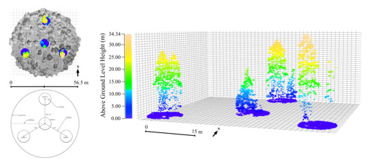
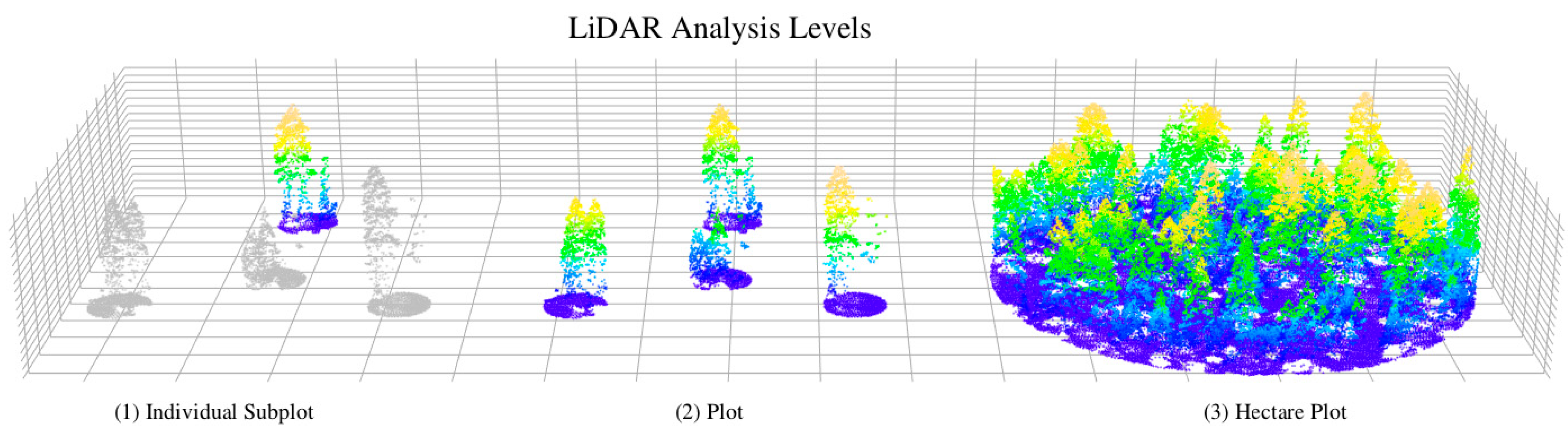
The overall objective of this study is to model forest AGBM and gV utilizing LiDAR metrics from individual subplots, four clustered subplots (hereafter referred to as a plot), and hectare plots using AGBM and gV estimates for individual subplots and plots calculated from ground-based FIA measurement data and regional allometric equations and subsequently compared to LiDAR-derived height percentile, height bin, and density bin metrics calculated for individual subplots, plots, and hectare plots. Plot AGBM and gV estimates were compared to plot and hectare plot LiDAR metrics as exhaustive tree tallies were not collected for the hectare plots. Since the data collected by ALS systems are capable of describing the three dimensional structure of the forest, they can be used to estimate forest biophysical parameters of interest such as AGBM and gV. Specific study objectives include: (1) development of a methodology to derive area-based airborne LiDAR metrics related to forest biophysical parameters for FIA subplots, plots, and hectare plots; (2) identification of relationships between the LiDAR metric sets and FIA subplot and plot estimates of forest AGBM and gV calculated using regional allometric equations; (3) investigation of the effectiveness of individual and multiple point cloud metrics to predict AGBM and gV within the context of the FIA plot design; and (4) identification of the most appropriate LiDAR metrics and analysis level for estimating AGBM and gV in the conditions present in the western forests in the US. While the remote sensing literature abounds with forestry LiDAR studies, our study brings novel elements that include: (1) development of an ALS-based methodology for estimating AGBM and gV utilizing the national forest inventory in the US, the USFS FIA plot design and ground measurements; (2) investigation of the effectiveness of previously developed point cloud metrics within the context of the FIA plot design; and (3) comparison of AGBM and gV estimates over three analysis scales: individual subplots (r = 7.32 m), plots (n = 4 subplots, each with r = 7.32 m), and hectare plots (r = 56.42 m).
3. Results
Individual SLR models were created for the AGBM and gV estimates using each of the point cloud-based metrics calculated for the individual subplots, plots, and the hectare plots. Diagnostic plots from the initial SLR models confirmed the existence of heteroscedasticity, and further examination found the histograms of the AGBM and gV data were positively skewed. Both issues violate the assumptions of linear regression, and indicate that the original models were not appropriate, and that a transformation was needed for the data to satisfy the normality and constant variance assumptions of linear regression. Such transformations are also commonly used to normalize positively skewed distributions and reduce heteroscedasticity [
55]. All SLR models were rerun using the natural log and square root transformed AGBM and gV data. Diagnostic plots indicated that the square root transformation (AGBM
sqrt and gV
sqrt) was most appropriate for these data.
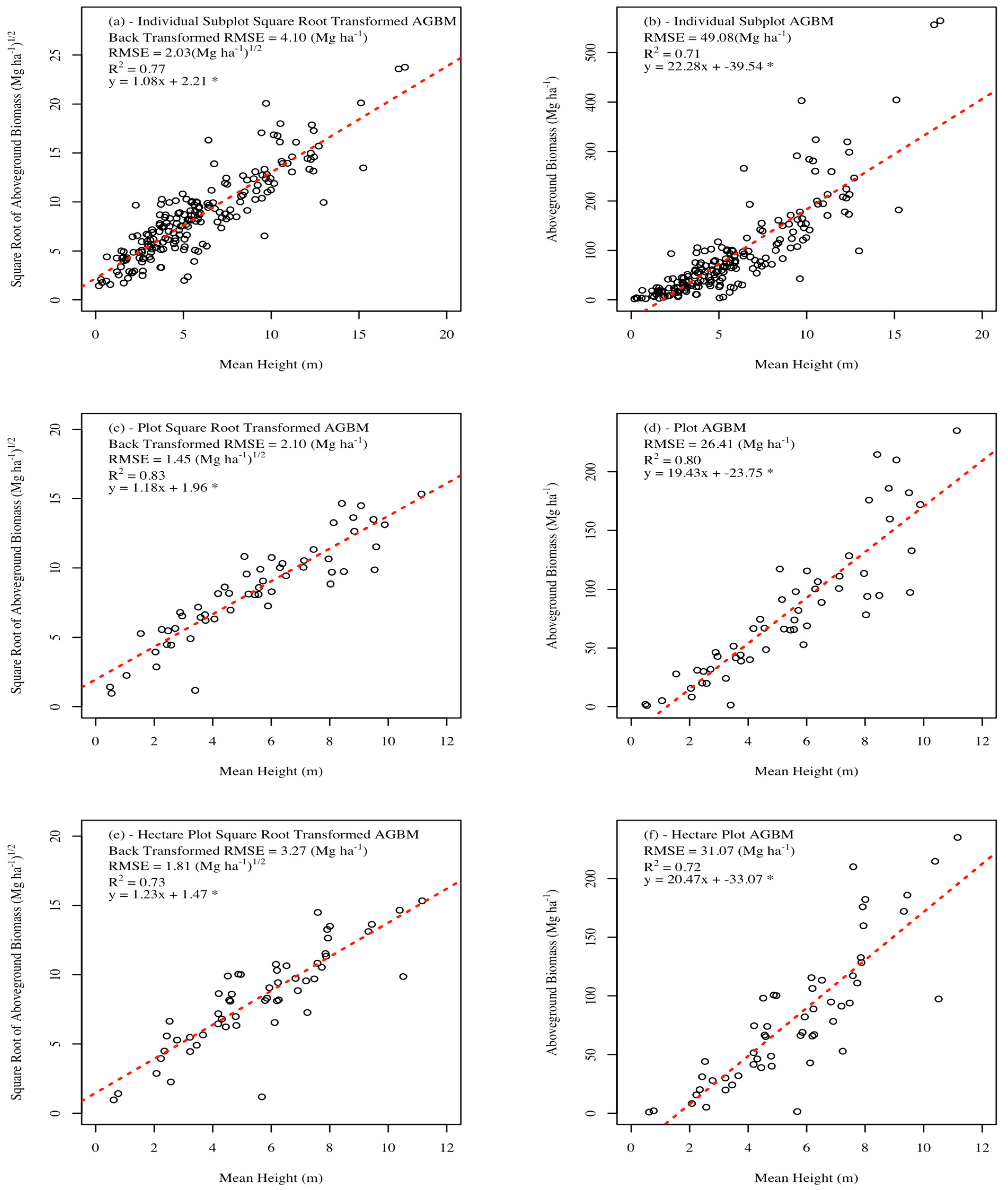
When utilizing the subplot square root transformed AGBM and gV data, the best independent variables from the independent subplot point cloud metric sets were: mean height (
Figure 7a and
Figure 8a), hb20-25, and d3, which accounted for 77%, 52%, and 67% of the variability in field estimated AGBM and 73%, 49%, and 62% of the variance in field estimated gV (
Table 7). All previously mentioned models were significant at the α = 0.05 level. The best independent variables for predicting AGBM from the plot point cloud metrics were also mean height (
Figure 7c), hb20-25, and d3, accounting for 83%, 56%, and 76% of the variability in field estimated AGBM. For gV, the best independent variables from the clustered subplot point cloud metrics were the p90 (
Figure 8c), mean height, hb20-25, and d3, accounting for 81%, 80%, 54%, and 74% of the variability in the field estimated gV. Mean height was also included in the best independent variable list since models produced using p90 and mean height were very similar (
Table 8). Models produced utilizing the plot point cloud metrics were all significant at the α = 0.05 level. The best independent variables for the hectare plot point cloud metric sets were mean height (
Figure 7e), hb15-20, and d3, accounting for 73%, 63%, and 73% of the variability in field estimated AGBM. The best independent variables for predicting gV from the hectare plot point cloud metric sets were p90 (
Figure 8e), hb15-20, and d3, accounting for 73%, 62%, and 71% of the variability in field estimated gV (
Table 9). Models for the hectare plot data were all significant at the α = 0.05 level.
Figure 7.
Scatter plot of simple linear regression results for the best simple linear regression aboveground biomass models (transformed and non-transformed) for individual subplots (a,b), plots (c,d), and hectare plots (e,f). * indicates p-values of less than 0.05.
Figure 7.
Scatter plot of simple linear regression results for the best simple linear regression aboveground biomass models (transformed and non-transformed) for individual subplots (a,b), plots (c,d), and hectare plots (e,f). * indicates p-values of less than 0.05.
Figure 8.
Scatter plot of simple linear regression results for the best simple linear regression gross volume models (transformed and non-transformed) for individual subplots (a,b), plots (c,d), and hectare plots (e,f). * indicates p-values of less than 0.05.
Figure 8.
Scatter plot of simple linear regression results for the best simple linear regression gross volume models (transformed and non-transformed) for individual subplots (a,b), plots (c,d), and hectare plots (e,f). * indicates p-values of less than 0.05.
Table 7.
Summary of the best subplot-level aboveground biomass and gross volume simple linear regression models for each point cloud metric set. * indicate p-values of less than 0.05.
Table 7.
Summary of the best subplot-level aboveground biomass and gross volume simple linear regression models for each point cloud metric set. * indicate p-values of less than 0.05.
| Subplot-Level |
|---|
| DV | IV | R2 | Adj-R2 | RMSE | β0 | β1 | PRESS |
|---|
| AGBMsqrt | mean | 0.77 | 0.77 | 2.03 | 2.21 * | 1.08 * | 819.56 |
| AGBMsqrt | hb20-25 | 0.52 | 0.52 | 2.94 | 6.11 * | 51.28 * | 1725.46 |
| AGBMsqrt | d3 | 0.67 | 0.67 | 2.45 | 1.70 * | 24.60 * | 1198.80 |
| gVsqrt | mean | 0.73 | 0.73 | 3.01 | 2.39 * | 1.44 * | 1812.01 |
| gVsqrt | hb20-25 | 0.49 | 0.49 | 4.16 | 7.61 * | 67.88 * | 3469.53 |
| gVsqrt | d3 | 0.62 | 0.62 | 3.57 | 1.77 * | 32.54 * | 2548.38 |
Table 8.
Summary of the best clustered subplot-level aboveground biomass and gross volume simple linear regression models for each point cloud metric set. * indicates p-values of less than 0.05.
Table 8.
Summary of the best clustered subplot-level aboveground biomass and gross volume simple linear regression models for each point cloud metric set. * indicates p-values of less than 0.05.
| Plot-Level |
|---|
| DV | IV | R2 | Adj-R2 | RMSE | β0 | β1 | PRESS |
|---|
| AGBMsqrt | mean | 0.83 | 0.83 | 1.45 | 1.96* | 1.18* | 119.73 |
| AGBMsqrt | hb20-25 | 0.56 | 0.56 | 2.31 | 5.57* | 63.59* | 305.42 |
| AGBMsqrt | d3 | 0.76 | 0.76 | 1.71 | 3.12* | 21.54* | 168.47 |
| gVsqrt | p90 | 0.81 | 0.81 | 2.05 | 0.49 | 0.65* | 237.39 |
| gVsqrt | mean | 0.80 | 0.79 | 2.12 | 2.26* | 1.15* | 258.30 |
| gVsqrt | hb20-25 | 0.54 | 0.54 | 3.18 | 7.01* | 83.90* | 578.31 |
| gVsqrt | d3 | 0.74 | 0.73 | 2.4 | 3.75* | 28.53* | 332.59 |
Table 9.
Summary of the best hectare plot-level aboveground biomass and gross volume simple linear regression models for each point cloud metric set. * indicates p-values of less than 0.05.
Table 9.
Summary of the best hectare plot-level aboveground biomass and gross volume simple linear regression models for each point cloud metric set. * indicates p-values of less than 0.05.
| Hectare Plot-Level |
|---|
| DV | IV | R2 | Adj-R2 | RMSE | β0 | β1 | PRESS |
|---|
| AGBMsqrt | mean | 0.73 | 0.73 | 1.81 | 1.47 * | 1.23 * | 186.49 |
| AGBMsqrt | hb15-20 | 0.63 | 0.63 | 2.12 | 3.16 * | 65.55 * | 254.03 |
| AGBMsqrt | d3 | 0.73 | 0.72 | 1.83 | 2.39 * | 23.65 * | 190.55 |
| gVsqrt | p90 | 0.73 | 0.72 | 2.45 | −0.47 | 0.68 * | 336.96 |
| gVsqrt | mean | 0.71 | 0.71 | 2.51 | 1.55 | 1.63 * | 364.11 |
| gVsqrt | hb15-20 | 0.62 | 0.61 | 2.92 | 3.81 * | 86.77 * | 482.64 |
| gVsqrt | d3 | 0.71 | 0.71 | 2.52 | 2.74 * | 31.51 * | 361.20 |
MR models for the subplot data were created utilizing independent variables selected with a mixed stepwise selection method (AIC criterion-based). The MR models showed only minor improvement in predictive ability when including more than one of the height percentile metrics. However, models based on multiple height bin metrics or multiple density metrics did improve the predictive ability of models (
Table 7 and
Table 10). The AGBM and gV MR models based on the height bin metric set included hb5-10, hb10-15, hb15-20, hb20-25, and hbgt25. All variables in both models were significant at the α = 0.05 level, and all VIFs were less than 10 indicating no multicollinearity issues. The height bin-based model was able to explain 78% of the variability in field estimated AGBM at the subplot-level. The height bin based gV MR model was able to explain 75% of the variability in gV. The MR model for predicting subplot AGBM from density metrics utilized d2, d3, d5, and d6, while the MR model for predicting subplot gV from density metrics utilized d2, d5, and d6. All model variables were significant at the α = 0.05 level, and VIFs were below 10. The MR models were able to explain 78% and 74% of the variance in field estimated AGBM and gV, respectively.
For MR models based on plot metric sets (
Table 11), the addition of multiple independent variables improved models for every metric set. Models utilizing percentile metrics as independent variables were able to account for the greatest variability in the field estimated AGBM and gV, 87% and 88%, respectively. The most notable improvement was seen in models utilizing height bin metrics, where the use of multiple height bin metrics allowed height bin-based models of AGBM and gV to account for 86% and 85% of the variability in the field estimated AGBM and gV, as compared to SLR models (utilizing hb20-25) which accounted for 56% and 54% of the variability in field estimated AGBM and gV. AGBM and gV models employing density metrics both utilized two density bins (d2 and d6), and were able to account for 86% and 84% of the variability in the field estimated AGBM and gV. All models reported in
Table 11 were significant at the α = 0.05 level, and showed no multicollinearity issues (all VIFs were lower than 10).
For MR models based on hectare plot metric sets, the addition of multiple independent variables only improved models based on height bin metrics or density metrics. The percentile-based MR models (for ABGM and gV) identified several independent variables (mean height and p90 for AGBM and mean height p90, and p25 for gV), but not all of the selected variables were significant at the α = 0.05 level, and had VIFs larger than 10 (indicating multicollinearity). The resulting model had a lower R2 value and higher RMSE than the SLR models developed for AGBM and gV SLR. The initial height bin-based MR model for AGBM (utilizing the square root transformation) utilized hb5-10, hb10-15, and hb15-20 as independent variables. This model showed no multicollinearity issues (VIFs below 10). All independent variables utilized were significant at the α = 0.05 level. The height bin-based model for gV (utilizing the square root transformation) employed hb10-15 and hb20-25, and showed no indication of multicollinearity (VIFs below 10). All independent variables were significant at the α = 0.05 level. The height bin-based MR models for AGBM and gV accounted for 74% and 73% of the variability in field estimated AGBM and gV, respectively. Analysis of the VIFs for the initial density-based MR models for the square root transformed AGBM and square root transformed gV did not indicate multicollinearity issues. All selected independent variables (d2 and d4 for AGBM and d2 and d5 for gV) were significant at the α = 0.05 level. Density-based MR models for AGBM and gV accounted for 75% and 73% of the variability in the field estimated AGBM and gV, respectively.
Modeling results presented above show that model R
2 values improved from models based on individual subplots to models based on plots. When the scale of the analysis level is increased to the hectare plot-level, a decrease in model R
2 values was observed. This pattern was visible in both SLR models and MR models (
Table 7,
Table 8 and
Table 9 and
Table 10,
Table 11 and
Table 12, respectively). Overall, the best R
2 values were obtained when using plot-level analysis.
Table 10.
Subplot-level multiple regression analysis results. * indicates p-values of less than 0.05.
Table 10.
Subplot-level multiple regression analysis results. * indicates p-values of less than 0.05.
| Subplot MR Models |
|---|
| DV | IV | R2 | Adj-R2 | RMSE | β0 | β1 | β2 | β3 | β4 | β5 | PRESS |
|---|
| AGBMsqrt | p90, mean | 0.78 | 0.78 | 1.99 | 1.58 * | 0.13 * | 0.85 * | NA | NA | NA | 802.77 |
| AGBMsqrt | hb5-10, hb10-15, hb15-20, hb20-25, hbgt25 | 0.78 | 0.77 | 2.02 | 2.85 * | 8.72 * | 11.47 * | 18.45 * | 17.81 * | 39.00 * | 832.19 |
| AGBMsqrt | d2,, d3, d5, d6 | 0.78 | 0.77 | 2.02 | 2.85 * | 11.58 * | 6.61 * | 20.64 * | −30.14 * | NA | 821.39 |
| gVsqrt | p95, max, mean | 0.75 | 0.75 | 2.93 | 2.83 * | 0.32 * | −0.21 * | 1.22 * | NA | NA | 1771.70 |
| gVsqrt | hb5-10, hb10-15, hb15-20, hb20-25, hbgt25 | 0.75 | 0.74 | 2.97 | 3.38 * | 9.77 * | 15.90 * | 26.42 * | 19.56 * | 54.08 * | 1789.31 |
| gVsqrt | d2, d5, d6 | 0.74 | 0.74 | 2.97 | 3.45 * | 21.18 * | 32.91 * | −46.42 * | NA | NA | 1775.36 |
Table 11.
Plot-level multiple regression analysis results. * indicates p-values of less than 0.05.
Table 11.
Plot-level multiple regression analysis results. * indicates p-values of less than 0.05.
| Plot MR Models |
|---|
| DV | IV | R2 | Adj-R2 | RMSE | β0 | β1 | β2 | β3 | β4 | PRESS |
|---|
| AGBMsqrt | p75, p95 | 0.87 | 0.87 | 1.26 | 1.03 | 0.32* | 0.23* | NA | NA | 97.33 |
| AGBMsqrt | hb5-10, hb15-20, hbgt25 | 0.86 | 0.85 | 1.32 | 2.09* | 19.91* | 33.74* | 58.81* | NA | 102.27 |
| AGBMsqrt | d2, d6 | 0.86 | 0.86 | 1.30 | 1.98* | 15.57* | 36.97* | NA | NA | 96.65 |
| gVsqrt | p25, p75, p95 | 0.88 | 0.88 | 1.63 | 0.93 | −3.25* | 0.46* | 0.06* | NA | 165.70 |
| gVsqrt | hb0-5, hb5-10, hb15-20, hbgt25 | 0.85 | 0.84 | 1.87 | 5.10* | −3.43* | 20.28* | 39.32* | 76.50* | 208.26 |
| gVsqrt | d2, d6 | 0.84 | 0.83 | 1.91 | 2.31* | 20.35* | 50.08* | NA | NA | 211.99 |
Table 12.
Hectare plot-level multiple regression analysis results. * indicates p-values of less than 0.05.
Table 12.
Hectare plot-level multiple regression analysis results. * indicates p-values of less than 0.05.
| | Hectare Plot MR Models |
|---|
| DV | IV | R2 | Adj-R2 | RMSE | β0 | β1 | β2 | β3 | PRESS |
|---|
| AGBMsqrt | hb5-10, hb15-20, hbgt25 | 0.74 | 0.73 | 1.82 | 1.83 * | 14.04 * | 48.68 * | 42.35 * | 189.49 |
| AGBMsqrt | d2, d4 | 0.75 | 0.74 | 1.77 | 1.67 * | 11.92 * | 15.67 * | NA | 178.87 |
| gVsqrt | hb10-15, hb20-25 | 0.71 | 0.71 | 2.53 | 2.55 * | 43.08 * | 83.40 * | NA | 365.18 |
| gVsqrt | d2, d5 | 0.73 | 0.72 | 2.45 | 1.38 | 21.16 * | 22.93 * | NA | 343.98 |
4. Discussion
Previous studies have found that ALS-derived variables describing the height of trees can produce accurate AGBM, gV, and other forest biophysical parameter predictions [
15,
16,
17,
18,
19,
20,
21,
22,
23,
24,
25,
26,
27]. To our knowledge, few studies have compared the ability of height percentile, height bin, and density LiDAR metrics to estimate AGBM and gV for the same dataset. In one such study, Næsset and Gobakken [
57] compare similar LiDAR metrics, but focused on forest growth using mean tree height, basal area, and volume under different forest conditions than those present in the Malheur National Forest. Our study is also unique in its analysis utilizing point cloud metrics from individual subplots, plots comprising a cluster of 4 subplots, and hectare plots to determine which dataset would best estimate AGBM and gV. Hectare plots were also utilized due to concern regarding geolocation and edge effect errors commonly associated with small area plots [
51,
52].
Table 5 provides descriptive statistics for the subplot center coordinates used to extract plot-level LiDAR data. Plot center GPS data utilized for this study exhibit superior geolocation precision when compared to the recreational-grade GPS receivers usually employed by FIA field crews.
After our analyses, it can be inferred that geolocation and edge effect errors did not have noticeable effect on the ability of subplot point cloud metrics to estimate AGBM and gV within our study area. However, future research efforts will attempt to quantify how geolocation and edge effect errors affected our AGBM and gV estimates. The best predictors of AGBM and gV at the individual subplot-level were mean height, hb20-25, and d3. Individual subplot SLR models based on hb20-25 exhibited a moderate relationship to AGBM and gV, while models based on d3 and mean height exhibited a stronger relationship. A visual examination of a subset of subplot point clouds identified that subplot-level mean height is commonly located near a high density cluster of LiDAR returns in the vertical distribution (as expected), while d3 typically covers a majority of the points within the upper forest canopy (
Figure 9). This suggests that mean height is an accurate predictor of AGBM and gV because it accurately describes tree height for the majority of trees on a plot. The d3 metric typically provides information on the taller trees within a plot, although in the presence of mostly short trees it may fail to capture such information (
Figure 9c,f). One possible reason for poor performance of SLR models based on subplot hb20-25 is the limited number of returns occurring within the 20–25 m. Thus, when larger trees are present within a plot this metric provides information useful for describing subplot-level AGBM or gV (since these trees will typically contain a large portion of the AGBM or gV within a subplot). However, when subplots contain trees less than 20 m tall, this metric essentially reports that no vegetation layers are present within a plot (
Figure 9b). This suggests that multiple height bin metrics might be required to correctly model AGBM and gV for forests with conditions similar to those exhibited in the Malheur National Forest. Our subplot MR models utilizing height bin-based independent variables (
Table 9) provide evidence for this finding, with the final model utilizing multiple height bin metrics, exhibiting no multicollinearity issues, and accounting for a similar amount of variance in field estimated AGBM and gV as the best subplot SLR models.
Overall, the plot SLR and MR models were able to account for the largest amounts of variability in the field estimate AGBM and gV (
Table 8). LiDAR-derived independent variables for the clustered subplot SLR models were mostly the same as those identified for the individual subplot models (mean, hb20-25, and d3). However, the best SLR model for gV utilized the percentile metric p90. This also occurred in the hectare plot SLR gV model. The SLR model utilizing the mean height value is very similar to the model based on p90, which is also similar to the SLR modeling results based on the hectare plot point cloud metrics.
Hectare plot-level SLR models utilizing height percentile metrics performed similarly to subplot-level SLR models, while density and height bin metric-based models were improved (
Table 9). The best SLR models in each point cloud metric set were mean, hb20-25, and d3 for AGBM and p90, hb15-20, and d3 for gV.
Table 9 also reports results for the gV model based on the mean, as this model was similar to the model based on p90. Models based on the previously mentioned independent variables accounted for 73%, 63%, and 73% of the variability in the field estimated AGBM and 75%, 62%, and 71% of the variability in field estimated gV. We believe this improvement is the result of scaling the subplot estimates of AGBM and gV to the hectare plot-level, since the average of conditions observed for four relatively small subplots would more closely resemble the conditions found within the larger hectare plot.
Figure 9.
Cross-sectional plots of two subplot point clouds displaying the location of the best aboveground biomass and gross volume predictor variables. The left subfigures identify the mean height for each example subplot. The middle subfigures identify the location of height bin 20-25 for each example subplot. The right subfigures identify the location of density 3 for each example subplot.
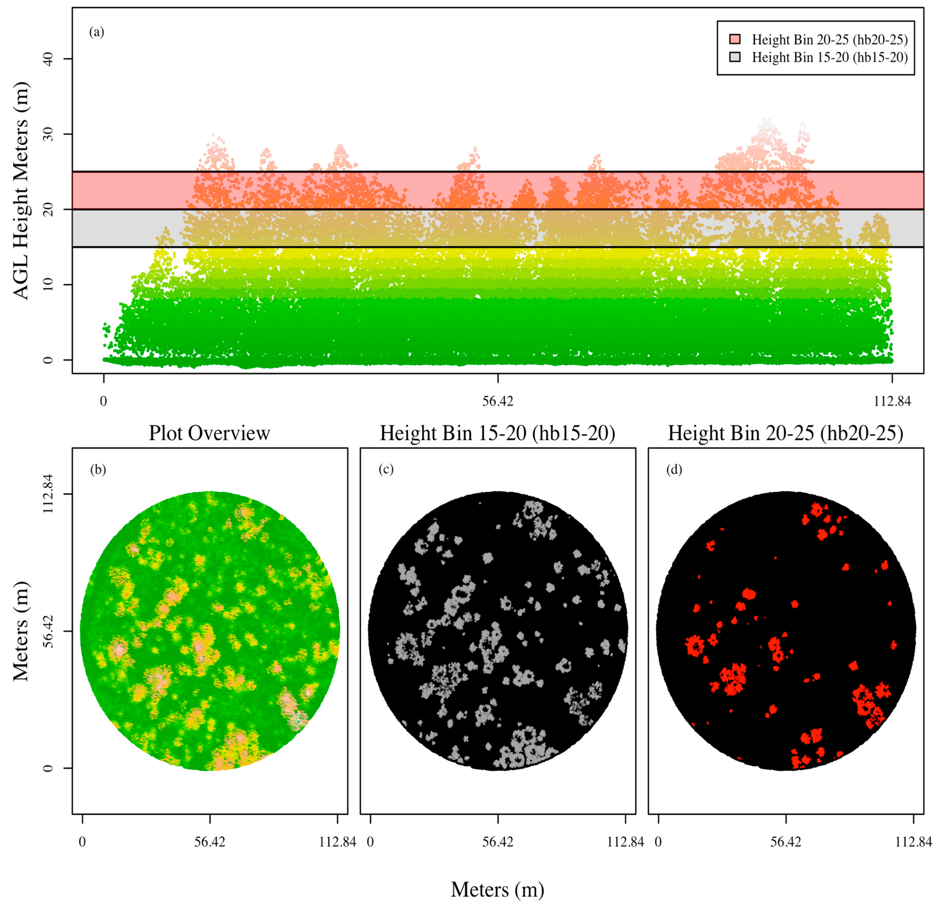
In some cases, the best plot and hectare plot-level SLR models for a given metric set utilized a different independent variable than the corresponding individual subplot-level SLR models. For example, the hectare plot-level height bin-based models for AGBM and gV models utilized hb15-20, while the subplot-level SLR utilized hb20-25. A visual examination of the two height bins in one of the hectare plots suggests that hb15-20 provides more information about the forest conditions on the hectare plot than hb20-25 (
Figure 10). This conclusion is also supported by the descriptive statistics for tree species height (
Table 3), which shows eight of the eleven tree species (including those composing the majority of trees within our plots) have mean heights within the hb15-20 range of 15 to 20 m.
Figure 10.
A visual comparison of height bin 15-20 and height bin 20-25 metrics for a hectare plot. Height bin15-20 provides more information about the conditions present on the hectare plot than height bin 20-25. (a) Cross sectional plot of one hectare plot and the location of height bin 15-20 and height bin 20-25; (b) Top-down representation of all points within the hectare plot; (c) Top-down representation of the points falling within height bin 15-20; and (d) Top-down representation of the points falling within height bin 20-25.
At the individual subplot-level, stepwise MR analysis identified that models based on height bin metrics and density metrics could benefit from multiple predictor variables, while improvements to models based on height percentile metrics were nearly negligible. In height bin and density-based models, the inclusion of multiple predictors increased the predictive ability of the models to a level similar to the mean height-based SLR model, with R2 values ranging from 0.74 to 0.78. AGBM and gV models utilizing height bin metrics always required more predictor variables than models utilizing density metrics, in part due to the compartmentalized nature of height bin metrics. Density metrics exhibit strong spatial correlation, and as such the inclusion of a large number of density bins leads to multicollinearity issues.
At the plot analysis level, stepwise MR analysis identified that models for each metric set could benefit from multiple predictor variables. While multiple independent variables were utilized in models for each metric set, a decrease in the number of variables in the height bin and density based models is observed. At the hectare plot-level, stepwise MR analysis identified that models utilizing height bin or density metrics would benefit from multiple predictor variables, while no additional predictor variables were identified for models based on height percentiles. However, it should be noted that density metric based models received only a minor improvement when a second predictor variable was added.
Results for the MR analyses show that point cloud metrics derived from the clustered subplots were able to account for the most variability in field estimated AGBM and gV, followed by models based on individual subplot metrics, and models based on hectare plot metrics. We hypothesize that the extent of hectare plot point cloud metrics was too large to adequately describe the average conditions present in the four subplots contained within each hectare plot. Future studies will investigate if a more appropriate plot size for LiDAR data covering the four subplots exists.
While subplot-level and hectare plot-level analyses produced adequate SLR and MR models, the best SLR and MR models were produced with the plot-level analysis. We believe there are several reasons why the plot level analysis produced the best results. When moving from subplot- to plot-level, the sample size is increased three-fold. If AGBM or gV is spatially distributed as a uniform random process, where tree locations approximating a Poisson simple point pattern and tree sizes approximating a distribution skewed to the right (considered to be the usual case) we expect estimation accuracy to increase rapidly with initial increases in sample size. However, when the spatial extent of the analysis is increased from the plot-level to the hectare plot-level we are forced to assume that the population is distributed identically within the hectare as within the subplots. This assumption might not be valid for all hectare plots utilizing the current field data, which was collected for each of the subplots. Thus, reductions in model R2 values are a result of the discrepancies in the population distribution between hectare plots and plots. Such discrepancies would not be an issue if exhaustive tree tallies were available for the hectare plots. Overall, this finding provides evidence that the current FIA plot design can be used with dense airborne LiDAR data to produce area-based estimates of AGBM and gV.
5. Conclusions
This study represents an initial attempt to model biophysical parameters of interest to the FIA program utilizing the standard FIA plot design, data from FIA ground crews, and ALS data. As previously mentioned, other studies have successfully modeled similar forest parameters with ALS data [
15,
16,
17,
18,
19,
20,
21,
22,
23,
24,
25,
26,
27,
34,
46,
49,
55]. However, to our knowledge none have done so for multiple analysis level (
i.e., subplot, plot, and hectare plot) comparing the performance of percentile, height bin, and density metrics, and specifically focused on modeling AGBM and gV for FIA purposes. Models based on subplot point cloud metrics, for AGBM and gV provided results similar to those presented in the literature and cited throughout this study.
Overall results from this study show that ALS can be used to create models that describe the AGBM and gV of Pacific Northwest FIA subplots with results comparable in accuracy to those of other published studies. Point cloud metrics based on PNW FIA hectare plots or individual subplots were not able to describe AGBM and gV as well as those based on plot point cloud metrics. The ability of ALS to collect data over large areas coupled with these results demonstrates the potential of ALS systems to augment current FIA data collection procedures by providing a temporary intermediate estimation of AGBM and gV for plots with outdated field measurements. We hypothesize that these intermediate estimates could prove beneficial for increasing the accuracy of forest C budgets by reducing variance caused by temporal measurement discrepancies in the currently available FIA measurements. However, more work must be done to quantify the amount of variance that would be reduced due to temporal measurement discrepancies, as well as the contribution of ALS-based estimates to this variance.
Future research identified by this study, includes: (1) utilization of regional species-specific growth and yield models to mitigate error caused by out-of-date tree measurements, while increasing the number of samples available for use in modeling efforts; and (2) investigations of how GPS accuracy and ALS data can be utilized to identify plots to be withheld from future modeling exercises.


