Moving Target Detection Based on the Spreading Characteristics of SAR Interferograms in the Magnitude-Phase Plane

Abstract

We propose a constant false alarm rate (CFAR) algorithm for moving target detection in synthetic aperture radar (SAR) images based on the spreading characteristics of interferograms on the magnitude-phase (M-P) plane. This method is based on the observation that, in practice, both moving and stationary targets along with clutter are located at different regions in the M-P plane, and hence reasonable partitions of the M-P plane can help in detecting moving targets. To ensure efficient CFAR detection and to resolve the effect of factors that influence detection results, the proposed algorithm is divided into three distinct stages: coarse detection, fine detection, and post-processing. First, to accurately describe the statistical behavior of clutter, a global censoring strategy, called coarse detection, is introduced to adaptively eliminate the influences of the moving and stationary target points from the given data. Then, to acquire fine detection results, a novel CFAR detector is developed on the basis of the fits of a known theoretical M-P joint probability density function (PDF) against the two-dimensional (2-D) histogram of the censored clutter. The joint PDF’s projected contour line that satisfies the desirable probability of false alarm (PFA) corresponds to the required threshold of detection in the M-P plane. Finally, two filters, the magnitude and phase filters, are applied to reduce the false alarms generated from the previous procedures. The effectiveness of the proposed algorithm is validated through experimental results obtained from a two-channel SAR complex image.

1. Introduction

Synthetic aperture radar (SAR) systems have become a popular tool for Earth observation over the last couple of decades because of their usability regardless of weather conditions [1]. At present, with the increase in the number of air- and space-borne dual- or multi-channel interferometric SAR sensors, ground moving target indication (GMTI) as an important aspect of SAR civilian and military applications is gaining widespread attention [2,3,4,5,6,7,8]. As the first step for GMTI, moving target detection plays a central role because accurate detection is crucial for post-processing that includes measurement of the target’s velocity [6,7], estimation of location, and focused imaging [3,8].

So far, many investigations have been conducted on moving target detection using dual- or multi-channel SAR images. Certain known schemes, such as space-time adaptive processing (STAP) [8,9,10,11,12], displacement phase center antenna (DPCA) [13,14], and along-track interferometry (ATI) [15,16], have demonstrated their usefulness in moving target detection. In addition, certain experiments and applications [17,18] have demonstrated that ATI has good potential for detecting ground-moving targets.

The key to using ATI for GMTI is to reasonably exploit the SAR interferogram, which is formed by multiplying the first image by the complex conjugate of the second one, i.e., the fore-channel signals by the aft-channel signals. The magnitude and phase (representing the phase difference between two-channel signals) in the SAR interferogram are useful for discriminating movers from the surrounding background clutter. Earlier ATI techniques [14,15,17] only utilized the phase difference between two channel images to extract moving targets because the stationary clutter can be cancelled in the interferometric phase domain, and the interferometric phase of a moving target is not equal to zero. However, this approach is not sufficient to achieve high detection performance because of the influences of phase excursion and random noise [17,18]. In practice, since a moving target can have a relatively higher radar cross section (RCS) than stationary clutter, which exhibits more dominant scattering intensity in the SAR images, the contribution of magnitude for detection of moving target cannot be ignored, especially in case of high resolutions [19]. Similarly, the adoption of only magnitude leads to limited detection because of the drawback that stationary targets, regarded as disturbances of the interested moving targets, also have high interferometric magnitude [19].

Considering the problems mentioned above, recent studies on moving target detection have combined magnitude and phase information, which is probably a trend of ATI technique development in the foreseeable future [19,20]. Unfortunately, since magnitude and phase are represented as two-dimensional (2-D) random signals and are not statistically independent [19], the combined statistical behavior of the interferometric magnitude and phase must be considered when one aims to devise a detection algorithm. In other words, the detection approaches should involve, directly or indirectly, the joint probability density function (PDF) of the interferometric magnitude and phase, following which, a suitable process, such as the constant false alarm rate (CFAR), can be applied to determine the detection threshold.

Studies, such as [20], have preliminarily demonstrated that analyzing the joint spreading characteristics in the magnitude-phase (M-P) plane is important for devising high-performance moving-target-detection algorithms. The characteristics of the statistical behavior of the magnitude and phase show that moving targets usually reside outside the 2-D joint histogram of the main clutter, and that the outer-most contour line in the M-P plane obtained from the projection of the joint histogram corresponds to the detection threshold. However, methods for developing an adaptive and reliable detection algorithm based on the spreading characteristics remain unclear.

In this study, we aim to develop an adaptive CFAR algorithm for moving-target detection based on the spreading characteristics of SAR interferograms in the M-P plane. The joint spreading characteristics in the M-P plane for targets and clutter are analyzed on the basis of the assumption that the detection threshold can be accurately identified if the statistical properties of clutter can be mathematically described by an appropriate theoretical M-P joint PDF. This theoretical distribution helps in developing a CFAR detector for flexible and adaptive detection of moving targets.

The technique outlined in this paper is unique and makes three contributions. Firstly, a global censoring strategy is introduced to eliminate the influences of the moving and stationary target points in the given data. Secondly, a novel CFAR detector is analytically derived and developed on the basis of the fits of a known theoretical M-P joint PDF against the 2-D histogram of the censored clutter. Finally, two filters, the magnitude and phase filters, are proposed to further reduce the false alarms.

This paper is organized as follows. In Section 2, a comprehensive analysis of the spreading characteristics of the target and clutter in the M-P plane is presented. Based on this analysis, the procedure for devising the detection algorithm is described in Section 3. Section 4 provides further algorithm details. We provide the experimental results of the proposed algorithm using typical measured SAR data in Section 5. The final section concludes this paper.

2. Spreading Characteristics of Target and Clutter in the Magnitude-Phase Plane

In this section, we analyzed the intrinsic spreading characteristics of different objects, such as moving targets, stationary targets, and background clutter, in the M-P plane. This analysis is important for guidance and as a foundation for constructing the detection algorithm presented in the following section. A simulated scene, including two moving point-targets with different radial velocities and one stationary point-target, from a dual-channel interferometric SAR system (the system parameters are the same as the one given in [19]) is employed, as shown in Figure 1, for considering a typical and ideal situation and thereby, draw some general conclusions. Figure 1a shows a simulated fore-channel magnitude SAR image where two moving targets with radial speeds of −4.0 m/s and 3.0 m/s are numbered 1 and 2, respectively (the minus denotes that the moving direction is inverse along the range axis). The values of the signal-to-clutter ratio (SCR) corresponding to these two moving targets are 5.25 dB and 4.32 dB, respectively. The value of the SCR relating to the stationary target 3 is 5.10 dB.

Figure 1. A typical SAR scene: (a) Simulated fore-channel SAR magnitude image; (b) The corresponding 2-D histogram.

Figure 1. A typical SAR scene: (a) Simulated fore-channel SAR magnitude image; (b) The corresponding 2-D histogram.

Figure 1b shows the 2-D histogram of the SAR interferogram of the simulated scene. The interferogram in the magnitude-versus-phase format resulting from the projection of this histogram in the M-P plane is shown in Figure 2a. The points coming from the moving targets, stationary target and clutter in the M-P plane are also labeled with different markers in this figure. From Figure 2a, we can draw the following general conclusions:

(1)

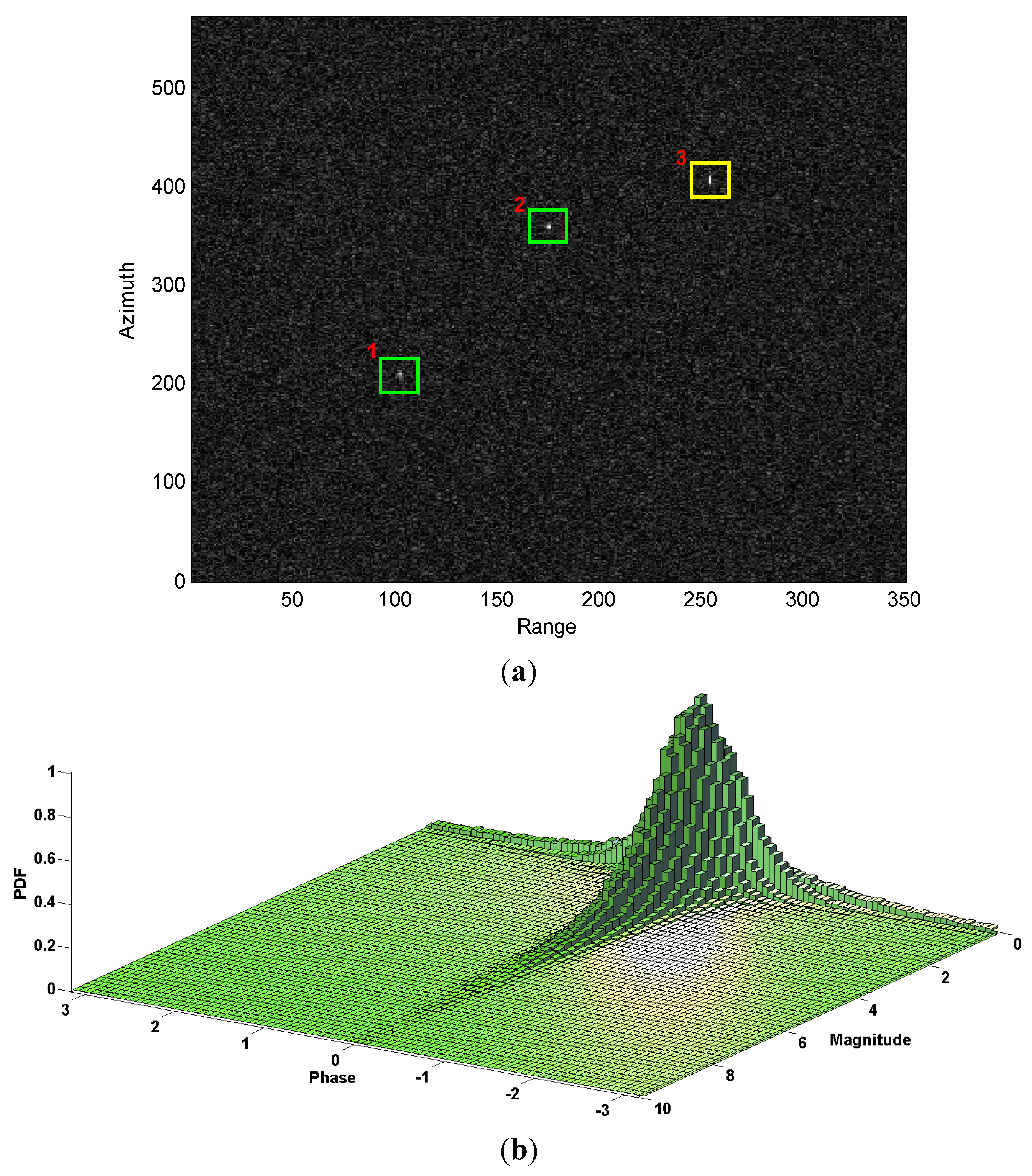
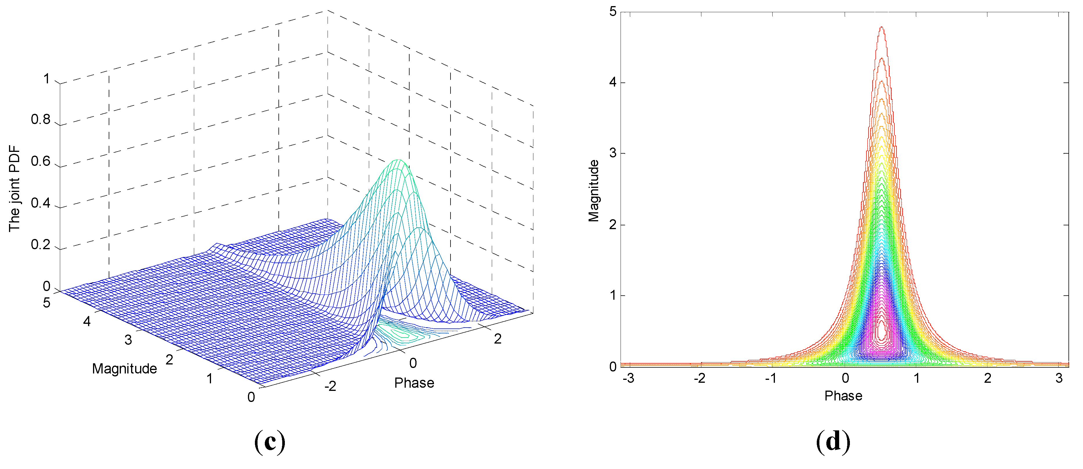
The clutter signals in the M-P plane of the interferogram are symmetric about a certain phase value θ, denoted as the central interferometric phase. This property is easy to understand because the phase differences of the clutter signals with the same interferometric magnitude deviate from a certain value in identical-probability, as also discussed in [21], when the number of clutter samples is sufficient. The θ is zero in most cases; however, it is not zero in certain situations, such as those with existing multi-scattering effects.

(2)

Both moving and stationary targets have a larger average power than the surrounding background, which results in a more dominant interferometric magnitude irrespective of whether the target is moving or stationary. The SCR depends on the distance between them and the stationary clutter in the M-P plane; a lower SCR will result if the stationary or moving targets are closer to the main clutter region in space.

(3)

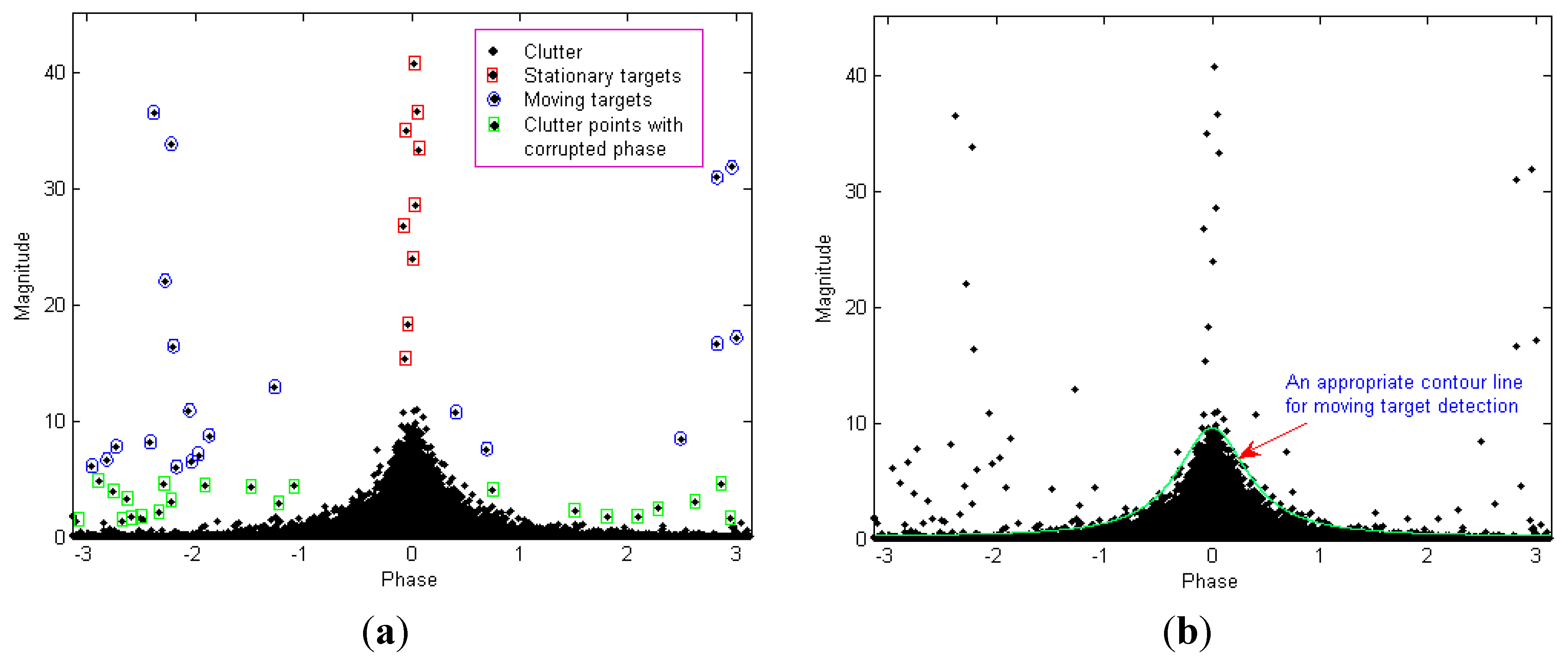
The interferometric phase of the stationary target is zero in ideal situations. In practice, the stationary target points concentrate on a very small phase interval at the position of the central interferometric phase due to certain disturbances of small phase noises. Contrarily, the moving target points tend to have larger interferometric phases that are deviated from the central phase owing to the presence of the target’s radial velocity. Additionally, the influences of phase excursion and random noise cause a few clutter points, which corrupts the interferometric phase to exhibit similar phase characteristics as the moving target points, although the magnitude of these clutter points is low.

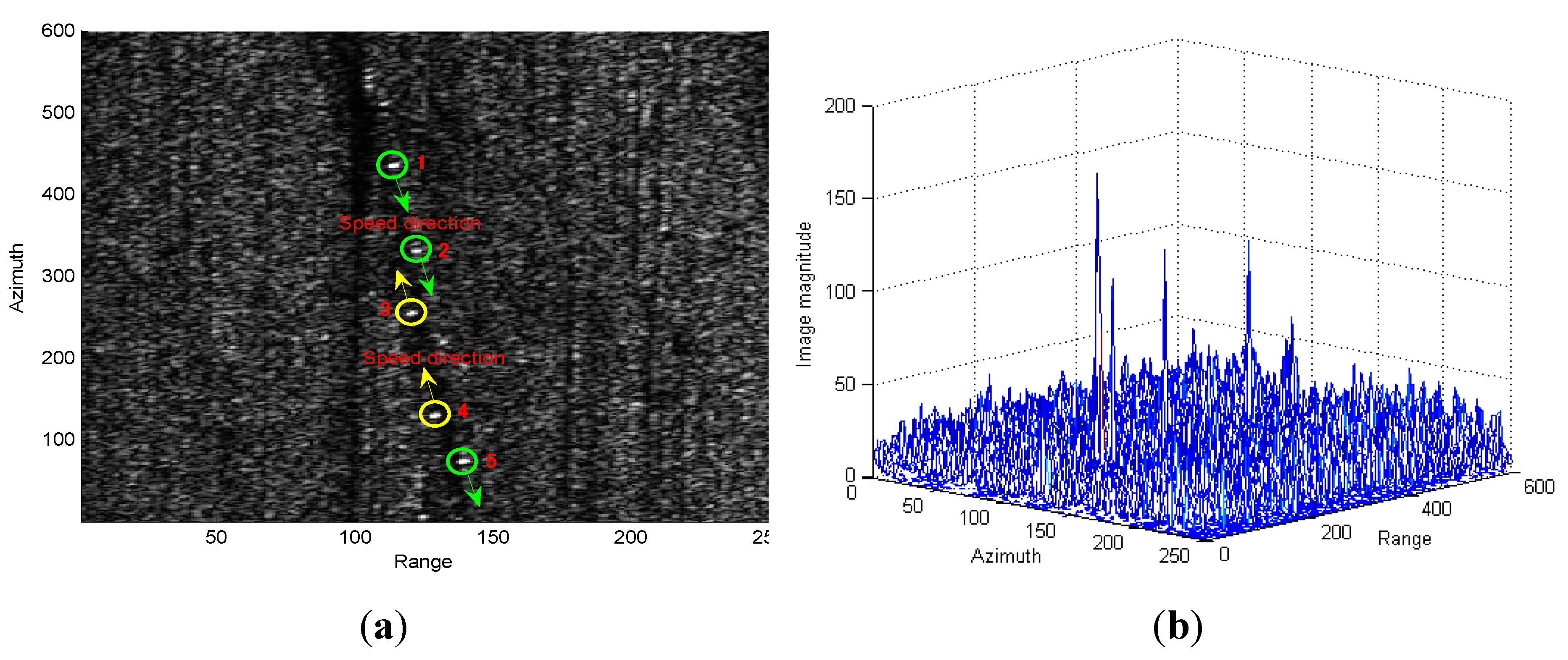
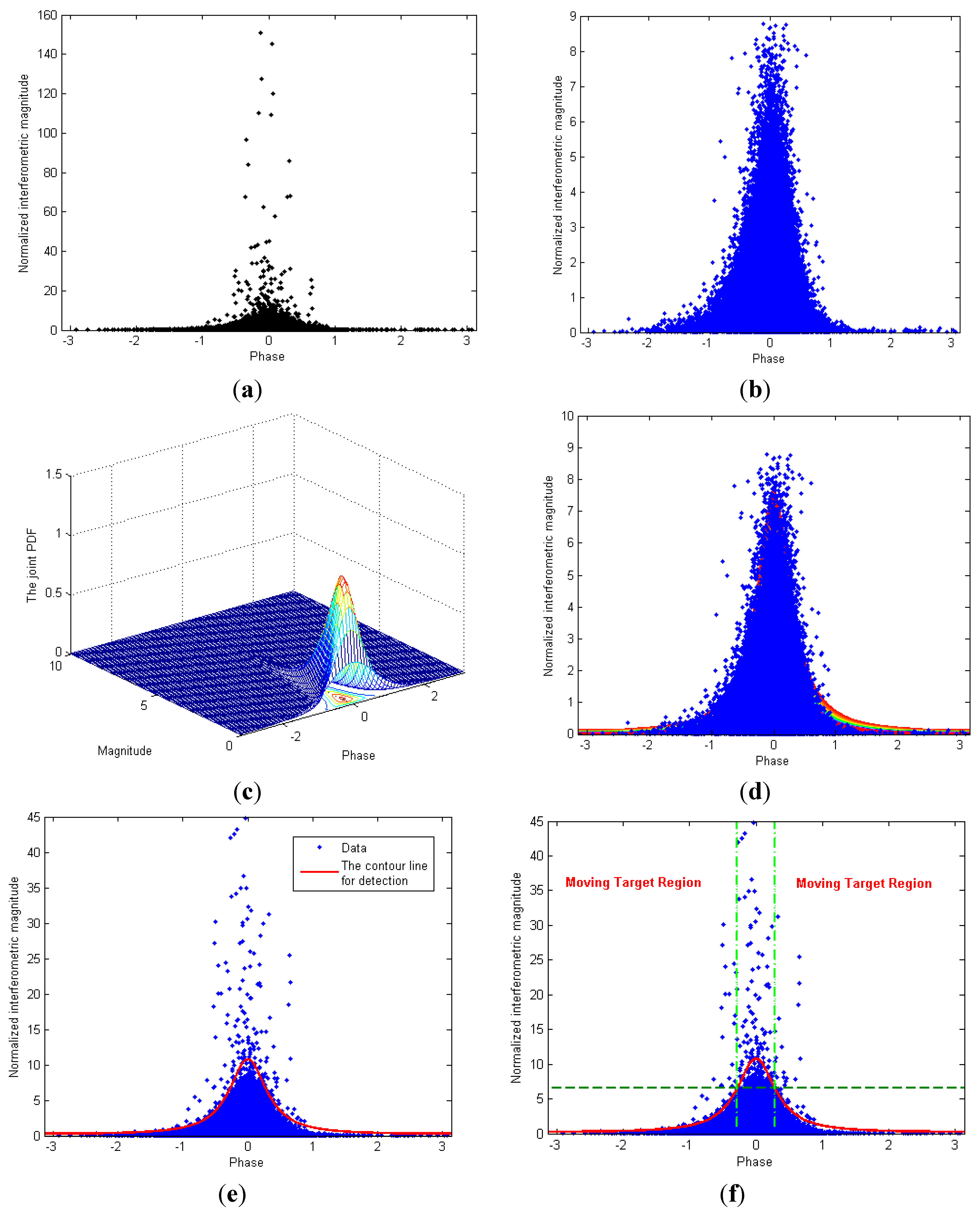
(4)

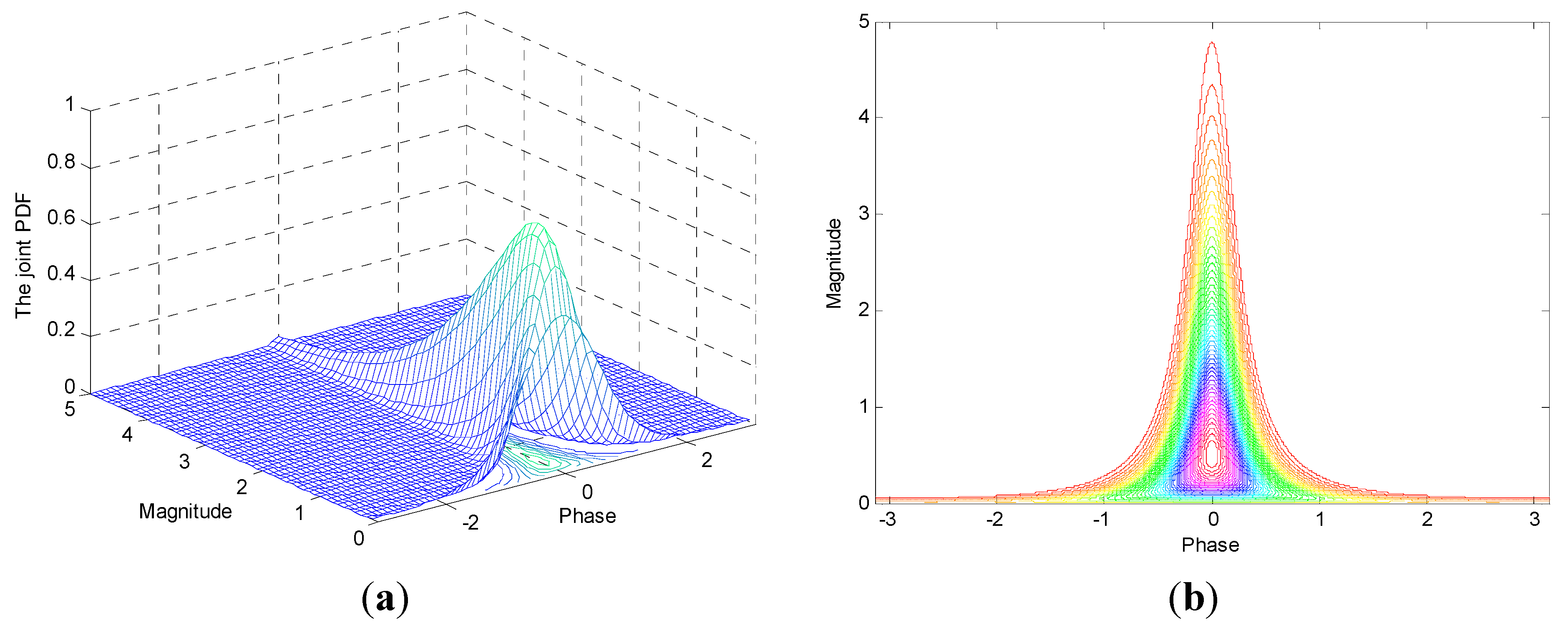
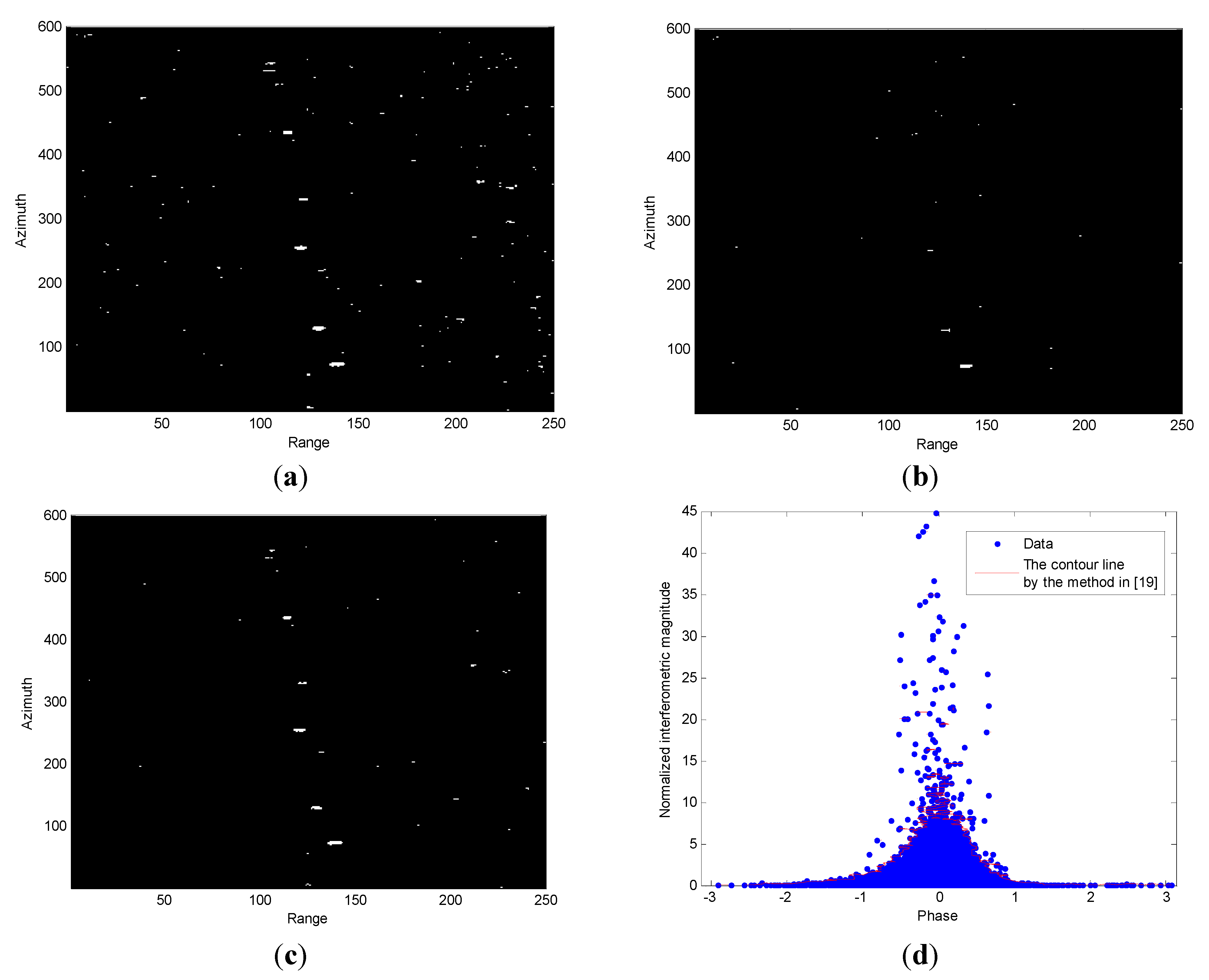
As shown in Figure 1b and Figure 2a, an appropriate contour line can cover the main clutter region, if we scan all contour lines with the projection of the 2-D histogram into the M-P plane. The appropriate contour line has the same height value in the 2-D histogram, which also represents the projection contour of the 2-D histogram’s different sections parallel to the M-P plane. This outer-most contour line is just the curve of the detection threshold, as shown in Figure 2b. From the viewpoint of statistical processing, the chief contributors to the clutter false alarms are the edge clutter points outside the line and the clutter points with corrupted interferometric phase.

Figure 2. The magnitude-phase (M-P) plane: (a) Magnitude vs. phase of SAR ATI signals: the moving target points whose phases are less than 0 belong to the target labeled 1 in Figure 1a; the moving target points whose phases exceed 0 belong to the target labeled 2 in Figure 1a; the stationary target points belong to the target labeled 3 in Figure 1a; (b) Sketch of the proper contour line to be used as the detection threshold.

Figure 2. The magnitude-phase (M-P) plane: (a) Magnitude vs. phase of SAR ATI signals: the moving target points whose phases are less than 0 belong to the target labeled 1 in Figure 1a; the moving target points whose phases exceed 0 belong to the target labeled 2 in Figure 1a; the stationary target points belong to the target labeled 3 in Figure 1a; (b) Sketch of the proper contour line to be used as the detection threshold.

3. Design of the Proposed Detection Algorithm

Inspired by the analysis of spreading characteristics in the M-P plane as mentioned above, several ideas can be used as the foundation for designing an actual moving target detection algorithm:

(1)

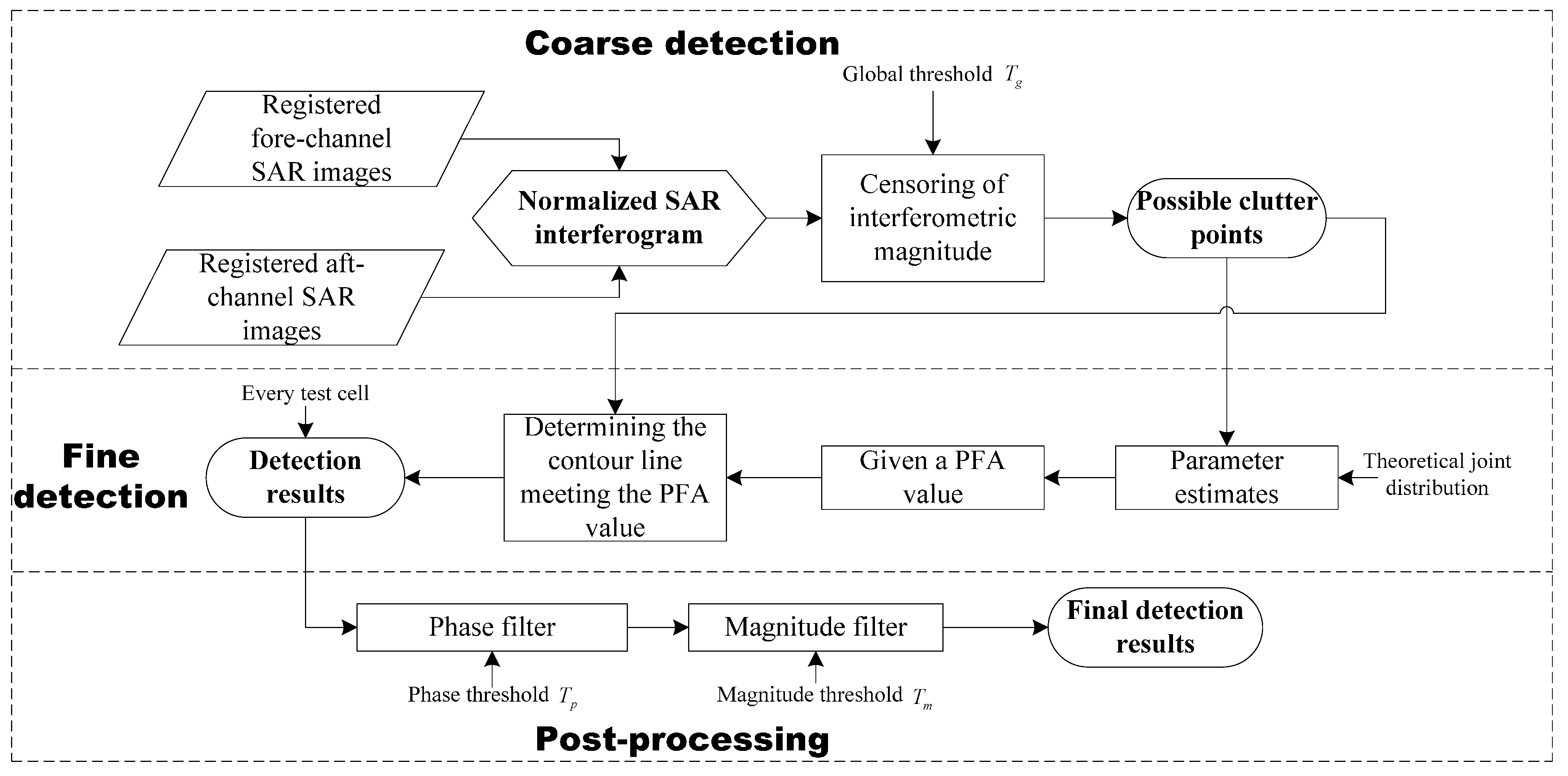
The central task for moving-target detection in the M-P plane is to determine the contour line containing the major power of the clutter. This contour line can be acquired either by analytical or empirical methods, as shown in [20]. The analytical method is more flexible and reliable than the empirical one because it does not require a complex and less-credible histogram-binning operation. Clearly, an effective and alternative approach to obtain the analytical expression of the detection contour line is to primarily derive the theoretical joint distribution of the interferometric magnitude and phase to match the 2-D histogram, and then apply a simple CFAR under a predefined PFA value.

(2)

To accurately describe the statistical behavior of clutter, it is necessary to eliminate the influences of the moving and stationary target points in the given data as much as possible before using the joint PDF to fit the 2-D histogram. This allows the proposed algorithm to have a real CFAR and can help us avoid the targets included in the detection curve (i.e., the over-fitting problem).

(3)

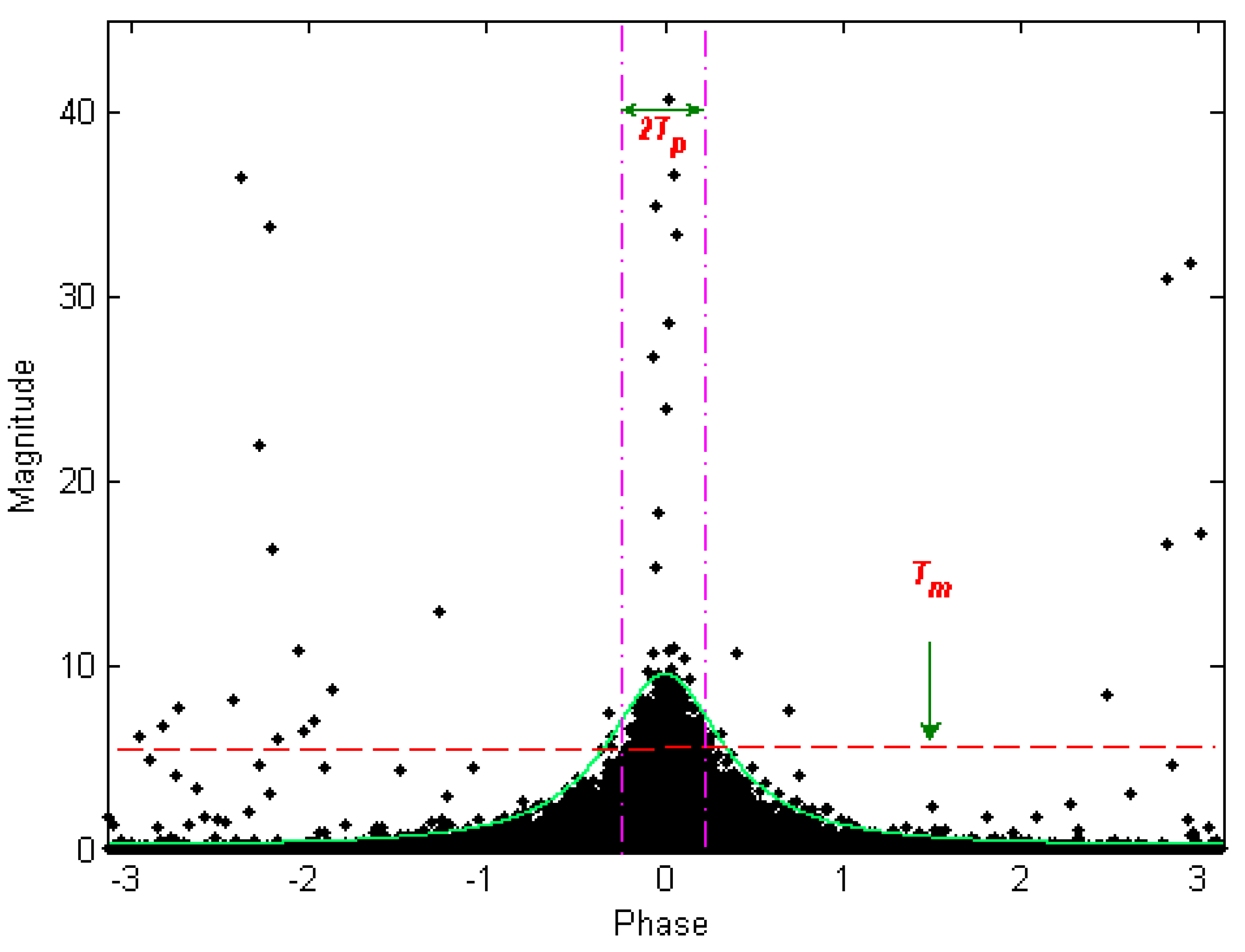
Even if a proper detection contour line can be given, various false alarms coming from two parts (one is clutter false alarms dominated by the corrupted-phase clutter points, and the other is generated by the stationary target points) should be emphasized. Accordingly, developing an effective method for removing false alarms is also worthy of consideration after CFAR processing.

The proposed detection algorithm was designed on the basis of the suggestions mentioned above. As seen in Figure 3, the whole flow of the proposed detection algorithm can be divided into three distinct stages: coarse detection, fine detection, and post-processing.

Figure 3. Flowchart of the proposed detection algorithm.

Figure 3. Flowchart of the proposed detection algorithm.

First, a coarse detection for the input normalized SAR interferogram is performed to remove the target’s influence on the statistical properties of clutter to gain high precision of parameter estimates in the theoretical joint distribution to match the observed 2-D histogram. Nevertheless, it should be noted that accurate separation of clutter and targets is almost impossible. Recently, Gao et al. [22] proposed a censoring strategy to overcome this type of coarse detection problem using a global threshold in accordance with a defined censoring depth. This method eliminates the disturbance of targets as much as possible. Some theoretical and experimental analyses [22] also demonstrate that this operation works well for proper selection of the global threshold in a wide range, permitting approximate selection of the global threshold. In this study, we adopt a similar process based on the fact that both moving and stationary targets have higher interferometric magnitude than clutter. In other words, if the magnitude of a pixel outperforms the global threshold T_g, it is labeled as a target point; otherwise, it is declared as a clutter point. Consequently, the possible clutter points can be censored out pixel by pixel from the normalized SAR interferogram.

Second, a fine detection is performed after the coarse detection. This detection begins from the parameter estimates of the theoretical joint PDF of magnitude and phase by making use of the possible clutter points. Then, immediately taking every possible clutter point into the analytical expression of the joint PDF, the value of the corresponding height, indicating a contour line to which the point belongs, is calculated. Under the condition of a predefined PFA, the expected detecting contour line can be acquired by a simple count, i.e., if the proportion of the number of clutter points, whose joint PDF value is less than a certain value, to the number of all the clutter points is identical to the given PFA, the contour line matching this value is the expected detection contour line. The fine detection results can be obtained by comparing the joint PDF value of all pixels in the entire interferogram with the expected detection contour line.

Figure 4. Illustration of the magnitude and phase filtering.

Figure 4. Illustration of the magnitude and phase filtering.

Finally, we complete the detection using post-processing, which mainly focuses on the reduction of false alarms. The disturbances coming from stationary targets are removed from the fine detection results by utilizing a phase filter with the threshold T_p under the assumption that the stationary target points generally have small interferometric phase value. The corrupted phase-clutter points caused by phase excursion and random noise are sequentially removed from the remaining detection results using a magnitude filter with a threshold T_m based on the assumption that most of these points have relatively low interferometric magnitude. An illustration of the magnitude and phase filters is shown in Figure 4.

4. Algorithm Details

4.1. Theoretical Joint Distribution

Given the fore-channel SAR complex signal z₁ and the aft-channel SAR complex signal z₂, the n-look sample covariance matrix is defined as the average of several independent samples [19,21], i.e.,

$$\widehat{R}=\frac{1}{n}{\displaystyle \sum }_{k=1}^{n}Z\left(k\right)Z{\left(k\right)}^H=\frac{1}{n}{\displaystyle \sum }_{k=1}^n\left[\begin{array}{cc}{\left|z_1\left(k\right)\right|}^2& z_1\left(k\right)z_2{\left(k\right)}^{*}\\ z_1{\left(k\right)}^{*}{z}_2\left(k\right)& {\left|z_2\left(k\right)\right|}^2\end{array}\right]$$

(1)

where n represents the number of looks, $Z\left(k\right)={\left[z_1\left(k\right),z_2\left(k\right)\right]}^T$ is the k^th single-look image, the superscript * represents the complex conjugate, and H refers to the complex conjugate transpose. The symbol $| |$ represents the modulus of the complex signal.

The off-diagonal elements $\frac{1}{n}{\displaystyle \sum }_{k=1}^n{z}_1\left(k\right)z_2{\left(k\right)}^{*}$ indicate the complex n-look interferogram. The normalized complex multi-look interferogram [19,21] is given by

$$I=\xi e^{j\psi }=\frac{\left(\frac{1}{n}\right){{\displaystyle \sum }}_{k=1}^n{z}_1\left(k\right)z_2{\left(k\right)}^{*}}{\sqrt{E\left({\left|z_1\right|}^2\right)E\left({\left|z_2\right|}^2\right)}}$$

(2)

where ψ indicates the multi-look interferometric phase and $\psi =arg\left\{\left(\frac{1}{n}\right){\displaystyle \sum }_{k=1}^n{z}_1\left(k\right)z_2{\left(k\right)}^{*}\right\}$, and E() denotes the expected value. The normalized multi-look interferometric magnitude is expressed as $\raisebox{1ex}{${\xi =\left(\frac{1}{n}\right)}^{\left|{{\displaystyle \sum }}_{k=1}^n{z}_1\left(k\right)z_2{\left(k\right)}^{*}\right|}$}\!\left/ \!\raisebox{-1ex}{$\sqrt{E\left({\left|z_1\right|}^2\right)E\left({\left|z_2\right|}^2\right)}$}\right.$.

In terms of the central limit theorem, the in-phase and quadrature components of each sample in z₁ or z₂ are independent and zero-mean complex Gaussian distributed when no scatterer is dominant in a resolution cell. According to [23], the random matrix $\mathit{B}=n\widehat{\mathit{R}}$ obeys the complex Wishart distribution

$$p_B\left(\mathit{B}\right)=\frac{\text{det}{\left(\mathit{B}\right)}^{n-2}\text{exp}\left[-tr\left({\mathit{C}}^{-1}\mathit{B}\right)\right]}{K\left(n,2\right)\text{det}{\left(\mathit{C}\right)}^n}$$

(3)

where $K\left(n,2\right)=\pi \Gamma \left(n\right)\Gamma \left(n-1\right)$, Γ() is the gamma function, and det() denotes the determinant operator.

Then, the underlying covariance matrix С [21] is

$$\mathit{C}=E\left[\mathit{Z}{\mathit{Z}}^H\right]=\left[\begin{array}{cc}{C}_{11}& \sqrt{C_{11}{C}_{22}}\rho e^{j\theta }\\ \sqrt{C_{11}{C}_{22}}\rho e^{-j\theta }& C_{22}\end{array}\right]$$

(4)

where ρe^jθ is the complex coefficient and ρ represents the magnitude of the complex correlation coefficients, $C_{11}=E\left({\left|z_1\right|}^2\right)$ and $C_{22}=E\left({\left|z_2\right|}^2\right)$.

We often assume θ to be zero on a ground scene [20]. However, it cannot be ignored in the presence of multi scattering effects in certain heterogeneous areas such as urban areas. In practical applications, the estimated $\widehat{\theta }$ of the parameter θ can be obtained from Equation (4).

According to Equation (3), Lee et al. [21] derived the mathematical expression of the joint distribution of the normalized interferometric magnitude ξ and the multi-look phase ψ

$$p_{\xi ,\psi }\left(\xi ,\psi \right)=\frac{2n^{n+1}{\xi }^n}{\mathrm{\pi }\mathrm{\Gamma }\left(n\right)\left(1-{\mathrm{\rho }}^2\right)}exp\left(\frac{2n\mathrm{\rho }\xi \cos \left(\psi -\theta \right)}{1-{\mathrm{\rho }}^2}\right)K_{n-1}\left(\frac{2n\xi }{1-{\mathrm{\rho }}^2}\right), \xi ,n>0, \rho \in (0,1], \psi \in (-\pi ,\pi ]$$

(5)

where K_{n – 1}() is the second type modified Bessel function with order n – 1.

The PDF defined by Equation (5) has the following characteristics [20,21]. First, it becomes narrow along the interferometric phase axis as n and ρ increases. Second, the density is symmetrical about θ. Resorting to the asymptotic formulas [24,25] of the modified Bessel functions, the resulting PDF of ξ can be easily derived as

$$p_{\xi }\left(\xi \right)=\frac{{\mathrm{\beta }}^n}{\mathrm{\Gamma }(n)}{\xi }^{n-1}\text{exp}\left(-\mathrm{\beta }\xi \right), \xi ,n,\mathrm{\beta }>0$$

(6)

with the parameter $\mathrm{\beta }=\frac{2n}{1+\mathrm{\rho }}$. The estimates $\widehat{\mathrm{\beta }}$ and $\widehat{n}$ correspond to the parameters β and n, respectively, and can be easily obtained with the help of numerical calculations based on the method-of-log-cumulants (MoLC) [26,27]:

$$\{\begin{array}{c}\Psi \left(\widehat{n}\right)-\ln \left(\widehat{\beta }\right)=\frac{1}{N}{\displaystyle \sum }_{i=1}^N\left[\ln (x_i)\right]=\widehat{\widetilde{c_1}}\\ \Psi \left(1,\widehat{n}\right)=\frac{1}{N}{\displaystyle \sum }_{i=1}^N\left[{(\ln (x_i)-\widehat{\widetilde{c_1}})}^2\right]\end{array}$$

(7)

where ψ() represents the digamma function (i.e., the logarithmic derivative of the Gamma function), ψ(r, ) is the r^th-order polygamma function (i.e., the r^th-order derivative of the digamma function), and $\left\{x_i\right\}, i\in \left[1, N\right]$ is a given sample set. $\widehat{\widetilde{c_1}}$ is the estimate of the first-order log-cumulant [26,27].

Figure 5 shows the plots of the joint PDF shown in Equation (5) with various parameters. It is evident that this density is symmetric about the central phase θ, and different values of θ result in a shift of the joint PDF or the contour line along the phase axis. Lee et al. [21] confirmed the effectiveness of the density, expressed by Equation (5), in fitting actual 2-D magnitude-phase histograms of clutter. In this study, we used this PDF to model the joint statistical characteristics of the interferometric magnitude and phase for the measured clutter data.

Figure 5. Joint distribution of the interferometric magnitude and phase: (a) The 2-D joint PDF with the parameters θ = 0, ρ = 0.9596 and n = 1; (b) The contour line of (a) in the M-P plane; (c) The 2-D joint PDF with the parameters θ = π/6, ρ = 0.9596, and n = 1; (d) The contour line of (c) in the M-P plane.

Figure 5. Joint distribution of the interferometric magnitude and phase: (a) The 2-D joint PDF with the parameters θ = 0, ρ = 0.9596 and n = 1; (b) The contour line of (a) in the M-P plane; (c) The 2-D joint PDF with the parameters θ = π/6, ρ = 0.9596, and n = 1; (d) The contour line of (c) in the M-P plane.

4.2. Global Threshold

As discussed previously, the pixels of moving targets and stationary targets generally have relatively larger interferometric magnitude values than clutter pixels. This permits the adaptive fixing of T_g by searching the magnitudes of all pixels in the interferogram. If the normalized interferometric magnitude ξ is regarded as a random variable under the condition that the confidence level of being a target pixel is 1 − ϕ, T_g can be determined from

$$P\left\{\xi >T_g\right\}=1-\varphi$$

(8)

where P is the probability, and ϕ ∈ [0,1], called the censoring depth [22], is an empirical value indicating the proportion of clutter pixels against the entire interferogram.

In most cases, ϕ is approximately 1 to ensure the presence of sufficient clutter pixels for parameter estimation. The probability P satisfying Equation (8) can be approximately obtained by the simple frequency statistics of the magnitude histogram.

4.3. CFAR Detector

After obtaining the possible clutter pixels in the interferogram, a CFAR detector for the following fine detection is required. Let ${\rm I}=\left\{I_i|I_i=\left({\xi }_i,{\psi }_i\right), 1\le i\le M\times N\right\}$ denote the column vector of the input $M\times N$ interferogram and $I_i=\left({\xi }_i,{\psi }_i\right)$ represent the interferogram value of the i-th pixel. According to the censoring, the remaining column vector of the interferogram for possible clutter points with the length R is assumed to be ${{\rm I}}_C=\left\{I_j|I_j=\left({\xi }_j,{\psi }_j\right), 1\le j\le R\right\}$. Moreover, plugging all possible clutter points into (5), the vector ${{\rm P}}_C=\left\{p_j|p_j=\left({\xi }_j,{\psi }_j\right), \left({\xi }_j,{\psi }_j\right)\in {{\rm I}}_C\right\}$ corresponding to the height value of each point against magnitude and phase can be obtained. The ${{\rm P}}_C$ elements are then sorted in the ascending order resulting in a sorted vector ${{{\rm P}}_C}^{\prime }=\left\{p_j|p_j\in {{\rm P}}_C, p_{j+1}\ge p_j\right\}$. Given a desirable PFA value, denoted by the symbol P_fa, the CFAR detection threshold T_CFAR can be analytically expressed by the following equation

$$T_{CFAR}={{{\rm P}}_C}^{\prime }\left(k\right), k=ceil(\left|{{{\rm P}}_C}^{\prime }\right|\bullet P_{fa})$$

(9)

where ${{{\rm P}}_C}^{\prime }\left(k\right)$ is the k-th element in the vector ${{{\rm P}}_C}^{\prime }$, ceil(x) is a ceiling operator for seeking the nearest integer greater than or equal to x, and $| |$ indicates the cardinality of the set (i.e., the number of elements in the set). The definition of Equation (9) is based on the following facts:

(1)

The movers are rare events in a dominant background of stationary clutter. They are outside the main clutter region and hence have low height values (i.e., the 2-D joint PDF value shown in Equation (5)). This implies that a clutter point with a lower height value is considered a more probable mover and produces a false alarm.

(2)

From the viewpoint of statistical processing, PFA can be defined as the ratio of the number of false alarms against the number of clutter points [1]. In other words, given a desirable PFA value Pfa, there must be k false alarms (see Equation (9)). Because ${{{\rm P}}_C}^{\prime }$ is a vector of height value and is arranged in the ascending order, the k^th element in the vector ${{{\rm P}}_C}^{\prime }$ is just the detection threshold matching P_fa.

We further define the function as

$$f\left(\xi ,\psi \right)=\frac{2n^{n+1}{\xi }^n}{\mathrm{\pi }\mathrm{\Gamma }\left(n\right)\left(1-{\mathrm{\rho }}^2\right)}\exp \left(\frac{2n\mathrm{\rho }\xi \cos \left(\psi -\theta \right)}{1-{\mathrm{\rho }}^2}\right)K_{n-1}\left(\frac{2n\xi }{1-{\mathrm{\rho }}^2}\right)-T_{CFAR}$$

(10)

The contour line with the identical T_CFAR value in the M-P plane is just the detection threshold curve. Therefore, each point (ξ,ψ) in the detection threshold curve satisfies the equation f(ξ,ψ) = 0. If a point falls outside the detection threshold curve, the corresponding function value of f(ξ,ψ) is less than zero.

Accordingly, for each test cell (ξ_i, ψ_i), 1 ≤ i ≤ M × N in the interferogram, the ground moving target is detected in this stage according to the following decision rule:

$$f({\xi }_i,{\psi }_i)\begin{array}{c}\begin{array}{c}{H}_0\\ >\end{array}\\ \begin{array}{c}<\\ H_1\end{array}\end{array}0$$

(11)

where H₁ is the hypothesis that the test cell is a target pixel, and H₀ is the hypothesis that the test cell is a stationary clutter pixel.

4.4. Removing False Alarms with Magnitude and Phase Filters

We used the phase filter to delete false alarms coming from stationary targets in the fine detection results. Under the assumption that the interferometric phases of stationary targets have low values, these values should fall within a small interval around the central phase θ. Therefore, a feasible and commonly-used phase threshold T_p for removing these false alarms of stationary targets is adopting the standard deviation σ_p of all the censored clutter-point phases, i.e.,

T_p =σ_p

(12)

When we take the interferometric phase of an element in the fine detection results as ψ_i, this element is considered a false alarm if the absolute value of ψ_i – θ is smaller than T_p.

After the phase filtering, the magnitude filter can be used to further reduce the false alarms coming from the corrupted-phase clutter points based on the assumption that most of these points have relatively low interferometric magnitude. To accomplish this task, we empirically defined a magnitude threshold T_m as

T_p = μ_m + λ∙σ_m

(13)

where μ_m and σ_m are the magnitude mean and standard deviation, respectively, of all the censored clutter points. λ is an adjusted experience parameter and is assigned an integer value greater than 1. If an output point from the previous processes has a lower magnitude than T_m, it is declared a false alarm.

5. Experimental Results of Measured Data

In this section, we validate the capability of the proposed CFAR detection of moving targets based on measured SAR data. The test dual-channel SAR data used in this investigation was acquired by a Chinese airborne SAR system operated in the X band and HH polarization, with a spatial resolution of 10 m × 2 m (azimuth × range) and size of 600 × 250 pixels. The location of the test site is near a highway in Beijing, dominated by shrubby vegetation. The fore-channel SAR magnitude image of the test site and a visible display of this image, are shown in Figure 6a,b. As shown in Figure 6a, five slowly moving cars, numbered 1–5, with opposite speed directions are travelling on this road.

Figure 6. Measured dual-channel SAR scene: (a) The fore-channel SAR image; (b) The visible display of (a).

Figure 6. Measured dual-channel SAR scene: (a) The fore-channel SAR image; (b) The visible display of (a).

The detection begins with generating the normalized interferogram using the complex signals of the two channels. All points in the interferogram are plotted in the phase-magnitude format as shown in Figure 7a, where each black solid dot in the M-P plane represents a complex-value element in the interferogram matrix. Next, we execute the proposed algorithm on this measured data step-by-step. The censoring of the interferometric magnitude is done in the first step. The global threshold T_g for the proposed algorithm was obtained with a confidence level of 1 – ϕ = 0.1%. The censoring results, indicating the possible clutter points, are shown in Figure 7b. Comparing Figure 7a,b, it is evident that most of the elements with high magnitude are eliminated from the primary data, which exhibits more focused spreading characteristics in the M-P plane and hence tends to follow a certain statistical distribution.

Figure 7. Detection in the M-P plane of the measured SAR data: (a) Magnitude vs. phase of the measured SAR complex signals; (b) The remaining censored clutter points in the M-P plane; (c) The theoretical PDF calculated to fit the 2-D histogram of the censored clutter; (d) The overlap display between the censored clutter and the M-P plane projection of (c,e). The obtained contour line for detection (Note: the vertical axis is plotted in a smaller range in contrast with (a) for better visualization); (f) The locked regions of moving targets by T_p, T_m as well as T_CFAR (Note: the vertical axis is plotted in a smaller range in contrast with (a) for better visualization).

Figure 7. Detection in the M-P plane of the measured SAR data: (a) Magnitude vs. phase of the measured SAR complex signals; (b) The remaining censored clutter points in the M-P plane; (c) The theoretical PDF calculated to fit the 2-D histogram of the censored clutter; (d) The overlap display between the censored clutter and the M-P plane projection of (c,e). The obtained contour line for detection (Note: the vertical axis is plotted in a smaller range in contrast with (a) for better visualization); (f) The locked regions of moving targets by T_p, T_m as well as T_CFAR (Note: the vertical axis is plotted in a smaller range in contrast with (a) for better visualization).

Based on the possible clutter pixels censored out, Figure 7c shows the estimated joint density expressed by Equation (5). The three contained parameters are estimated to be $\widehat{\theta }=-7.55\times {10}^{-16}$, $\widehat{n}=1.5774$ and $\widehat{\rho }=0.9387$. Furthermore, the overlap display between the censored clutter and the projection of the estimated joint PDF to the M-P plane is shown in Figure 7d. From Figure 7d, it is clear that the density shown in Equation (5) agrees well with the measured clutter from a visible viewpoint, which demonstrates the efficacy of this statistical model and the parameter estimates of the proposed method. By taking the theoretical false alarm probability as P_fa = 6 × 10⁻⁴, the corresponding detection contour line with identical threshold T_CFAR = 1.4907 × 10⁻⁶ is obtained, as shown in Figure 7e. This curve encircles most of the power of clutter. In the post-processing stage, consisting of a phase filter with a magnitude of one, the moving target regions are obtained in the M-P plane, as shown in Figure 7f. The two filtering thresholds are T_m = 6.5016 and T_p = 0.2816, and the adjusted parameter λ is empirically set as the integer 6. We must stress that λ cannot be adaptively selected at present. In practice, a small λ value will lead to some false alarms from clutter with low scattering magnitude that cannot be removed. In contrast, a large λ value will exclude most of the false alarms, but it can also cause partial loss of information of a moving target. However, if the moving targets have sufficient contrast with respect to the clutter, a large λ value can be selected because this will permit the detection of moving targets and help remove the clutter false alarms significantly. λ is set at 6 in this study because all the five moving targets in Figure 6a are sufficiently bright with respect to the background clutter.

Based on the partition of the M-P plane, as shown in Figure 7f, the detection results in different stages are shown in Figure 8. Figure 8a shows the binary images after the detection using the contour line shown in Figure 7e. The targets and false alarms are counted as follows: First, each 8-connected cluster of bright pixels in the binary images after the detection is labeled and counted as one region. This means that each bright pixel in one region must be located within 8-neighborhood of another specific bright pixel in this region. Second, if any point in a region is found to exist within a distance of 10 m from a ground truth position, the target is declared as found, and the region is regarded as the target region. All regions near a ground truth position of a target are counted as a target. All other detected regions that are not considered to be related to a target are regarded as false alarms. A connected cluster of false alarm pixels in an 8-neighborhood is counted as one false alarm. As a consequence, the fine detection using the contour line, as shown in Figure 8a, obtains the intact contour of the moving targets, while also producing 28 false alarms. A comparison of Figure 6a and Figure 8a shows that these false alarms come from the stationary clutter points with relatively strong backscattering and the clutter points with corrupted interferometric phase. Two filters were used to clear up these false alarms step-by-step in the post-processing. Figure 8b,c shows the binary images after applying the phase and magnitude filters, respectively. As shown in Figure 8b, the phase filter removes false alarms from the stationary clutter points with relatively strong backscattering. Twenty one false alarms remain after applying the phase filter (note that some false alarms cannot be visualized because they occupy very few pixels). In Figure 8c, more false alarms from the clutter points with the corrupted interferometric phase are excluded. In summary, Figure 8a–c clearly exhibit the manner in which the proposed algorithm detects moving targets and removes false alarms. Each step leads to reduced false alarms, although partial moving target points are also lost. Based on this flow, the final detection results corresponding to the original SAR image is shown in Figure 8d. It is easy to observe that all five moving targets are detected without any false alarm, which proves the effectiveness of the proposed CFAR detection method for detecting moving targets.

Figure 8. Detection results of the proposed method: (a) Binary output with the detection contour line; (b) Binary results after applying the phase filters; (c) Results after applying the magnitude filter; (d) Detection results corresponding to the original SAR image.

Figure 8. Detection results of the proposed method: (a) Binary output with the detection contour line; (b) Binary results after applying the phase filters; (c) Results after applying the magnitude filter; (d) Detection results corresponding to the original SAR image.

In [20], a CFAR method with a similar concept of M-P plane partition to detect moving targets was reported. This method is rather attractive because: on the one hand, certain experiments [20,28,29] have suggested the performance superiority of the method by comparing with conventional ATI techniques, e.g., [30], and classical DPCA approach [29]; on the other hand, the method in [20] was also considered as a candidate technique for RADARSAT-2 commercial SAR satellite to carry out the GMTI measurements [28,29]. Hence, to further assess the performance of the proposed method, we compared it with the method reported in [18]. Instead of deriving the theoretical joint PDF of clutter, the technique in [20] estimated the joint PDF through a 2-D histogram binning procedure. The main drawback of the method in [20] is that the detection results strongly depend on the bin size (or equivalently, the number of bins), and hence are not stable and credible. This is understandable because the estimated joint PDF always varies with the bin size. In theory, if there are sufficient clutter samples, a smaller bin size will lead to a better approximation of the estimated PDF against the true one. However, clutter samples are always limited in practice. A large bin number corresponds to a small bin size and a fine PDF approximation, which results in many bin cells with very few clutter points. This implies that many bin cells containing clutter points have low height values in the 2-D histogram and can be easily misclassified and produce false alarms. In contrast, a small bin number corresponds to a large bin size and a coarse PDF approximation, and target points can be easily incorporated into the surrounding clutter points in the 2-D histogram as a bin cell, which results in target points with large height values that are judged as clutter (i.e., the targets are missed). Therefore, an appropriate bin size is important for the performance of the detection in the method in [20]. However, it is rather challenging because it is not possible to know the proper bin size for detection prior to the task. It is also unrealistic to exhaustively seek all bin sizes to obtain an optimal size.

Figure 9. Detection results of the method in [20]: (a) Binary output with the bin numbers at 2000 × 100 (range × azimuth); (b) Binary output with the bin numbers at 100 × 50 (range × azimuth); (c) Binary output with the bin numbers at 1000 × 50 (range × azimuth); (d) The obtained contour line for detection in (c).

Figure 9. Detection results of the method in [20]: (a) Binary output with the bin numbers at 2000 × 100 (range × azimuth); (b) Binary output with the bin numbers at 100 × 50 (range × azimuth); (c) Binary output with the bin numbers at 1000 × 50 (range × azimuth); (d) The obtained contour line for detection in (c).

The detection results shown in Figure 9 verify the former analysis. Given the same theoretical false alarm probability as Figure 8 and Figure 9a,b show the detection results of the method in [20] under bin numbers 2000 × 100 (range × azimuth) and 100 × 50 (range × azimuth), respectively. The former generates 161 false alarms and the latter generates 31 false alarms, but target number 3 is almost missed. The experimental results shown in Figure 9a,b agree well with the previous analysis; that is, the method in [20] is not stable and credible and that the detection performance strongly relies on the manual selection of bin size. A good detection result is obtained when the bin numbers are set at 1000 × 50 (range × azimuth), as shown in Figure 9c. The corresponding contour line of detection for the method in [20] is given in Figure 9d. The detection results of Figures 8a and Figure 9c are similar because all targets are clearly detected; however, the method in [20] produces a slightly large number of false alarms (51 false alarms). The magnitude and phase filters in the proposed algorithm can further exclude the false alarms. In summary, based on the results shown in Figure 8 and Figure 9, the method proposed in this study is superior to the method proposed in [20].

6. Conclusions

We developed a CFAR detection algorithm for detecting moving targets in SAR images based on the spreading characteristics of interferograms in the M-P plane. The method is based on the idea that reasonable partitions in the M-P plane can show moving target regions in terms of the spreading characteristics. The presented algorithm is divided into three distinct stages: coarse detection, fine detection, and post-processing. In the coarse detection stage, a global censoring threshold is introduced to adaptively eliminate the influences of the moving target and stationary target points on the statistical behavior of the clutter. Next, a novel CFAR detector that uses a known theoretical M-P joint PDF to match the 2-D histogram of the censored clutter is proposed. The central task of this detector is to obtain a contour line satisfying the desirable PFA in the M-P plane. Subsequently, two filters are applied to reduce false alarms. We have also demonstrated that the proposed CFAR algorithm is effective by performing our experiments on a typically measured two-channel SAR complex image.

The appropriate method for selecting the adjusted parameter λ in an adaptive way still needs to be determined; it is empirically set at present. It might be obtained by analysis of more real data. Further tests and assessments of the proposed algorithm are required. This should be done in future studies, given the abundance of collected data.

References

1. Oliver, C.J.; Quegan, S. Understanding Synthetic Aperture Radar Images; Artech House: Norwood, MA, USA, 1998. [Google Scholar]
2. Steyskal, H.; Schindler, J.K.; Franchi, P.; Mailloux, R.J. Pattern synthesis for TechSat21-A distributed space-based radar system. IEEE Antennas Propag. Mag. 2003, 45, 19–25. [Google Scholar] [CrossRef]
3. Raney, R.K. Synthetic aperture imaging radar and moving targets. IEEE Trans. Geosci. Remote Sens. 1971, 3, 499–505. [Google Scholar]
4. Schulz, K.; Soergel, U.; Thoennessen, U. Segmentation of moving objects in SAR-MTI data. Proc. SPIE. 2001, 4382, 174–181. [Google Scholar]
5. Moreira, A. Real-time synthetic aperture radar (SAR) processing with a new sub-aperture approach. IEEE Trans. Geosci. Remote Sens. 1992, 30, 714–722. [Google Scholar] [CrossRef]
6. Liu, C.; Gierull, C.H. A new application for PolSAR imagery in the field of moving target indication/ship detection. IEEE Trans. Geosci. Remote Sens. 2007, 45, 3426–3436. [Google Scholar] [CrossRef]
7. Wang, G.; Xia, X.; Chen, V.C. Dual-speed SAR imaging of moving targets. IEEE Trans. Aerosp. Electron. Syst. 2006, 42, 368–379. [Google Scholar] [CrossRef]
8. Kirscht, M. Detection and imaging of arbitrarily moving targets with single-channel SAR. IEE Proc. Radar Sonar Navig. 2003, 150, 7–11. [Google Scholar] [CrossRef]
9. Guerci, J.R.; Goldstein, J.S.; Reed, I.S. Optimal and adaptive reduced-rank STAP. IEEE Trans. Aerosp. Electron. Syst. 2000, 36, 647–663. [Google Scholar] [CrossRef]
10. Koch, W.; Klemm, R. Ground target tracking with STAP radar. IEE Proc. Radar. Sonar Navig. 2001, 148, 173–185. [Google Scholar] [CrossRef]
11. Wang, Y.; Chen, J.; Bao, Z. Robust space-time adaptive processing for airborne radar in nonhomogeneous clutter environments. IEEE Trans. Aerosp. Electron. Syst. 2003, 39, 70–81. [Google Scholar] [CrossRef]
12. Barbarossa, S.; Farina, A. Space-time-frequency processing of synthetic aperture radar signals. IEEE Trans. Aerosp. Electron. Syst. 1994, 30, 341–358. [Google Scholar] [CrossRef]
13. Maori, D.C.; Klare, J.; Brenner, A.R.; Ender, J.H.G. Wide-area traffic monitoring with the SAR/GMTI system PAMIR. IEEE Trans. Geosci. Remote Sens. 2008, 46, 3019–3030. [Google Scholar] [CrossRef]
14. Entzminger, J.N. JointSTARS and GMTI: Past, present and future. IEEE Trans. Aerosp. Electron. Syst. 1999, 35, 748–761. [Google Scholar] [CrossRef]
15. Moccia, A.; Rufino, G. Spaceborne along-track SAR interferometry: Performance analysis and mission scenarios. IEEE Trans. Aerosp. Electron. Syst. 2001, 37, 199–213. [Google Scholar] [CrossRef]
16. Chapin, E.; Chen, C.W. Along-track interferometry for ground moving target indication. IEEE Aerospace Electron. Syst. Mag. 2008, 23, 19–24. [Google Scholar] [CrossRef]
17. Livingstone, C.; Thompson, A. The moving object detection experiment on RADARSAT-2. Can. J. Remote Sens. 2004, 30, 355–368. [Google Scholar] [CrossRef]
18. Fienup, J.R. Detecting moving targets in SAR imagery by focusing. IEEE Trans. Aerosp. Electron. Syst. 2001, 37, 794–809. [Google Scholar] [CrossRef]
19. Shi, G.; Zhao, L.; Wang, N.; Gao, G.; Chen, Q.; Liu, A.; Kuang, G. A novel dual-SAR detector based on the joint metric of interferogram’s magnitude and phase for slow ground moving targets. Proc. SPIE 2009, 7471, 538–543. [Google Scholar]
20. Chiu, S. A constant false alarm rate (CFAR) detector for RADARSAT-2 along-track interferometry. Can. J. Remote Sens. 2005, 31, 73–84. [Google Scholar] [CrossRef]
21. Lee, J.S.; Hoppel, K.W.; Mango, S.A.; Miller, A.R. Intensity and phase statistics of multilook polarimetric and interferometric SAR imagery. IEEE Trans. Geosci. Remote Sens. 1994, 32, 1017–1028. [Google Scholar] [CrossRef]
22. Gao, G.; Liu, L.; Zhao, L.; Shi, G.; Kuang, G. An adaptive and fast CFAR algorithm based on automatic censoring for target detection in high-resolution SAR images. IEEE Trans. Geosci. Remote Sens. 2009, 47, 1685–1697. [Google Scholar] [CrossRef]
23. Goodman, N.R. Statistical analysis based on a certain multivariate complex Gaussian distribution (an introduction). Ann. Math. Stat. 1963, 34, 152–180. [Google Scholar] [CrossRef]
24. Gradshteyn, S.I.; Ryzhik, I.M. Table of Integrals, Series, and Products, 7th ed.; Academic Press: San Diego, CA, USA, 2007. [Google Scholar]
25. Previato, E. Dictionary of Applied Math for Engineers and Scientists; CRC Press: London, UK, 2003. [Google Scholar]
26. Abdelfattah, R.; Nicolas, J.M. Interferometric SAR coherence magnitude estimation using second kind statistics. IEEE Trans. Geosci. Remote Sens. 2006, 44, 1942–1953. [Google Scholar] [CrossRef]
27. Nicolas, J.M. Introduction to second kind statistic: Application of log-moments and log-cumulants to SAR image law analysis. Trait. Signal. 2002, 19, 139–167. [Google Scholar]
28. Livingstone, C.; Sikaneta, I.; Gierull, C.H.; Chiu, S.; Beaudoin, A.; Campbell, J.; Beaudoin, J.; Gong, S.; Knight, T.A. An airborne synthetic aperture radar (SAR) experiment to support RADARSAT-2 ground moving target indication (GMTI). Can. J. Remote Sens. 2002, 28, 794–813. [Google Scholar] [CrossRef]
29. Chiu, S.; Livingstone, C. A comparison of displaced phase centre antenna and along-track interferometry techniques for RADARSAT-2 ground moving target indication. Can. J. Remote Sens. 2005, 31, 37–51. [Google Scholar] [CrossRef]
30. Gierull, C.H. Statistical analysis of multilook SAR interferograms for CFAR detection of ground moving targets. IEEE Trans. Geosci. Remote Sens. 2004, 42, 691–701. [Google Scholar] [CrossRef]