Article

Shiftable Leading Point Method for High Accuracy Registration of Airborne and Terrestrial LiDAR Data

1
Jiangsu Provincial Key Laboratory of Geographic Information Science and Technology, Nanjing University, Nanjing 210093, China
2
Collaborative Innovation Center for the South Sea Studies, Nanjing University, Nanjing 210093, China
3
Collaborative Innovation Center of Novel Software Technology and Industrialization, Nanjing University, Nanjing 210093, China
4
Department of Geographic Information Science, Nanjing University, Nanjing 210093, China
5
Jiangsu Center for Collaborative Innovation in Geographical Information Resource Development and Application, Nanjing 210023, China
*
Authors to whom correspondence should be addressed.
Remote Sens. 2015, 7(2), 1915-1936; https://doi.org/10.3390/rs70201915
Submission received: 10 November 2014 / Accepted: 29 January 2015 / Published: 9 February 2015
(This article belongs to the Special Issue Lidar/Laser Scanning in Urban Environments)

Abstract

:
A new automated approach to the high-accuracy registration of airborne and terrestrial LiDAR data is proposed, which has three primary steps. Firstly, airborne and terrestrial LiDAR data are used to extract building corners, known as airborne corners and terrestrial corners, respectively. Secondly, an initial matching relationship between the terrestrial corners and airborne corners is automatically derived using a matching technique based on maximum matching corner pairs with minimum errors (MTMM). Finally, a set of leading points are generated from matched airborne corners, and a shiftable leading point method is proposed. The key feature of this approach is the implementation of the concept of shiftable leading points in the final step. Since the geometric accuracy of terrestrial LiDAR data is much better than that of airborne LiDAR data, leading points corresponding to anomalous airborne corners could be modified for the improvement of the geometric accuracy of registration. The experiment demonstrates that the proposed approach can advance the geometric accuracy of two-platform LiDAR data registration effectively.

Graphical Abstract

1. Introduction

Light detection and ranging (LiDAR), as a measuring means of acquiring three-dimensional data, is able to provide detailed and accurate irregular point clouds of object surfaces [1]. A variety of LiDAR techniques have emerged, and LiDAR data are often acquired from various platforms, for example airborne [2,3], mobile [4,5] and terrestrial platforms [6,7]. Acquiring data from a side view, terrestrial LiDAR can obtain detailed facade information of objects at relatively high resolution. However, its scanning range is limited, and the top information of objects is usually missing [8]. Conversely, airborne LiDAR obtains data from a top view, where there is abundant top information; however, the facade and side information is limited, and the spatial resolution is relatively low. Considering the advantages and disadvantages of the data collected from these two platforms, their integration has become inevitable [9]. In recent years, a growing amount of research has focused on the integration of these two datasets for various applications, e.g., topographic mapping [10], geological exploration [11], forest research [12], hydrologic survey [13], 3D reconstruction [14] and virtual reality [15].
In order to combine airborne and terrestrial LiDAR data for certain applications, the registration of these two datasets is required. However, huge differences exist between them. In particular, compared with airborne LiDAR data, terrestrial LiDAR data have the following characteristics. (1) Higher geometric positioning accuracy: in general, the horizontal and vertical positional accuracy of airborne LiDAR data collected by common commercial systems is around the decimeter level; however, terrestrial LiDAR can achieve geometric positioning accuracy up to the millimeter level. (2) Higher spatial resolution: hundreds (or even thousands) of meters away from objects, the resolution of airborne LiDAR data is at the meter or decimeter level; terrestrial LiDAR data can achieve much higher spatial resolutions within tens of meters away from objects. (3) Different point of view: because airborne LiDAR obtains data from a top view, it includes more top information and less side information; conversely, terrestrial LiDAR obtains data from a horizontal or a bottom view, resulting in detailed side information and relatively little top information. Thus, it is difficult to achieve automatic registration of high geometric accuracy between these datasets, owing to the various differences between them.
In this study, a new approach is proposed for the automatic registration of two-platform LiDAR data in environments characterized by dense buildings, where building features, especially building corners, are used. The proposed approach primarily consists of the following steps. (1) Extraction of building corners from airborne LiDAR data (referred to as airborne corners) and terrestrial LiDAR data (known as terrestrial corners): building contours are derived from airborne LiDAR data and terrestrial LiDAR data, respectively; building corners are extracted through the intersection of the obtained contours. (2) Initial matching of the airborne and terrestrial corners: a matching technique based on maximum matching corner pairs with minimum errors, referred to as MTMM, and in which conjugate airborne and terrestrial corners are found, is introduced in this study. (3) The shiftable leading point method for the improvement of the geometric accuracy of registration: terrestrial corners are used as referenced data, and leading points are generated from airborne corners; a shiftable leading point method is proposed to shift the leading points from their original positions to their corresponding terrestrial corners. Note that an airborne point cloud is taken as a rigid body, and single airborne corners are not moved from the airborne point cloud. Then, the shifted leading points are registered with the terrestrial corners, leading to the final registration of LiDAR data from two platforms.
The key objective of this approach lies in the shiftable leading point method for the improvement of the geometric accuracy of registration. Due to following reasons, the extracted airborne corners may be of relatively low geometric accuracy and include numerous anomalous corners: (1) the accuracy of airborne footprints may vary due to the range error, GPS locating error, INS attitude error, etc.; (2) due to the large average point spacing, actual building contours may be located between two neighboring scan lines, on the base of which the extracted building contours will deviate; (3) constrained by algorithms for extracting building contours and corners, errors may exist more or less. Compared with airborne corners, the terrestrial corners are of relatively high accuracy with extremely few anomalous corners. Based on the above consideration, it is a problem to combine the large amount of airborne corners of low geometric accuracy with anomalous corners and the few terrestrial corners of high geometric accuracy for a high accuracy registration. During a registration procedure, the registration accuracy is influenced by the amount, distribution and geometric accuracy of conjugate features. When faced with few conjugate features, it is not feasible to filter the features for the inliers, e.g., the RANSAC (random sample consensus) algorithm [16], which may do great harm to the distribution of the original features. RANSAC is an iterative method to estimate the parameters of a mathematical model from a set of observed data that contains outliers. The basic assumption of RANSAC is that the sample contains correct data (inliers, i.e., data whose distribution can be explained by some set of model parameters) and abnormal data (outliers, i.e., data that do not fit the model). To address above problems, in this paper, a shiftable leading point method is proposed. High accuracy terrestrial corners are used as referenced data, and leading points are generated from airborne corners. The basic idea of this method is to eliminate the inner relative error of anomalous leading points according to the terrestrial corners through an iterative shifting procedure. In this way, the general distribution of conjugate features is retained with relatively high accuracy.

2. Related Work

2.1. Review on Registration of LiDAR Data from the Same Platform

In recent years, registration of LiDAR point clouds has drawn increasing attention. Related studies can mainly be grouped into two aspects: (1) registration of multi-scan terrestrial LiDAR data; and (2) strip registration of airborne LiDAR data.

2.1.1. Registration of Multi-Scan Terrestrial LiDAR Data

In the registration of multi-scan terrestrial LiDAR data, two main approaches can be found based on the utilized features, i.e., range-based registration and image-based registration. In the former approaches, geometric features, like points, lines and planes, are used. For the purpose of forestry applications, Hilker et al. [17] set up bright reference targets as tie-points. Liang et al. [18] also utilized artificial masks for point cloud registration. Wang [19] proposed a block-to-point fine registration approach, where the point clouds are divided into small blocks, and each block is estimated as a representative point. Besides points, lines are also used for point cloud registration. Jaw and Chuang [20] provided a workflow for multi-scan terrestrial LiDAR data registration using line features. More recently, after a global registration of point clouds, Bucksch and Khoshelham [21] extracted skeletons from tree branches and exploited the matching of these skeletons. Plane features for registration can be found in [22], where single plane correspondences are used to solve the transformation parameters with some additional assumptions. Stamos and Leordeanu [23] suggested a registration technique with planes and lines extracted from range scans. Zhang et al. [24] fit planes from segmented point clouds and utilized the characteristic of the Rodriguez matrix to establish a mathematical model of registration. In addition, Bae and Lichti [25] evaluated the change of the geometric curvature and the approximate normal vector of the local surface, which are then used for the registration of two partially overlapping point clouds. Geometric curvature and the normal vector of points can also be found in some approaches [26,27,28].
Spectrum information (e.g., intensity and RGB values), as a common by-product during the scanning process, provides additional information for point cloud registration [29]. Al-Manasir and Fraser [30] obtained digital images using a camera mounted on a terrestrial laser scanner and used scale-invariant feature transform (SIFT) to solve the transformation relationship with the co-planarity model. Instead of SIFT features, speeded-up robust features (SURF) were extracted in [29], which were later used to solve the transformation parameters with a linear transformation technique. Not only camera images, but also reflectance images are good supplementary information for point cloud registration. Based on an algorithm for the least squares matching of overlapping 3D surfaces, Akca [31] provided an extension algorithm that can simultaneously match surface geometry and its attribute information. Reflectance images were also used to help the registration of terrestrial LiDAR data in many associated research works [32,33,34].

2.1.2. Registration of Airborne LiDAR Strips

In the strip registration process of airborne LiDAR data, geometric features are often used. Schenk et al. [35] described two mathematical models to find the optimal transformation parameters, in which the first model minimizes the remaining difference along the Z-axis and the second model minimizes the distance between points to patches. Maas [36] presented a formulation of least squares matching based on a triangulated irregular network (TIN), which can effectively avoid the degrading effects caused by interpolation. Based on surfaces from photogrammetric procedures, Bretar et al. [37] proposed a methodology for the adjustment problem of the airborne laser scanner strip, in which aerial images over the same area are needed. Lee et al. [38] employed lines to measure and adjust the discrepancies between overlapping LiDAR data strips, in which TINs are created for the segmentation of points and line equations are determined from the intersection of neighboring planar patches. Habib et al. [39] presented three alternative methodologies for the internal quality control of parallel LiDAR strips using pseudo-conjugate points, conjugate areal and linear features and point-to-patch correspondence, respectively.
Considering the characteristic disparity of the point cloud from a terrestrial platform or airborne platform, the registration task usually works in two steps: rough registration and fine registration. In the process of fine registration, the iterative closest point (ICP) algorithm presented in [40] is used most widely, in which an iterative estimation of transformation parameters between two overlapping point clouds is conducted to converge to a local minimum. Variants of ICP were then proposed [41,42,43,44]. In spite of the improvement, in general, ICP demands good initial alignments of point clouds for the convergence of the local minimum.

2.2. Review of the Registration of Airborne and Terrestrial LiDAR Data

Research on the registration of point cloud data concentrates primarily on the registration of data from the same platform, particularly for the registration of multi-scan terrestrial LiDAR. Consequently, detailed information regarding the registration of point cloud data from different platforms is lacking. Among the existing studies, many researchers have conducted the registration of airborne and terrestrial LiDAR data with the aid of auxiliary data, such as GPS and remotely-sensed images, by directly utilizing the geographic coordinates of terrestrial LiDAR data as control points [11,45].
The use of feature primitives, such as points, lines and planes, is another important method for the registration of two-platform LiDAR data; however, few previous studies have investigated this or related subjects. Line primitives were used in [46] to register airborne and terrestrial LiDAR data. One three-dimensional sphere with a specific radius was constructed for each LiDAR point; then, LiDAR points along building contours were determined based on the points inside the sphere. The angles of the contours were analyzed, after which, rotation and translation matrices were calculated through a random test-selection strategy. The use of line primitives provides a feasible way for the registration of point cloud data; however, in many complex situations, the registration result may not be sufficiently stable, limited by the completeness and accuracy of the extracted line features. Jaw and Chuang [15] constructed a multi-feature conversion model for the integrated utilization of point, line and plane features to lead to automatic registration. Bang et al. [1] calibrated the airborne LiDAR system using terrestrial LiDAR data as the reference data. In this process, point and plane features were utilized to conduct an initial registration; subsequently, precise registration was conducted using the ICP algorithm. The combination of these two methods allowed the integrated utilization of multiple features for the registration of airborne and terrestrial point clouds. However, there has been little study of the extraction of feature primitives, a process that is directly related to the final result of registration. In fact, the quality and geometric accuracy of extracted features also varies greatly, owing to the disparity between airborne and terrestrial point cloud data. Therefore, the effective extraction of accurate features and the appropriate use of these features in high-quality registration have yet to be achieved.

3. Method

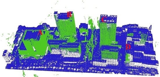
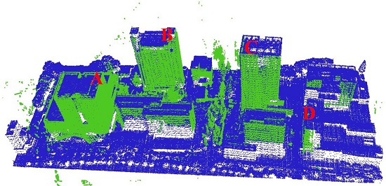
3.1. Extraction of Building Corners from Airborne and Terrestrial LiDAR Data

Airborne LiDAR data provide abundant top information of building roofs, from which reliable building contours can be derived for the extraction of airborne corners (Figure 1a). Here, building contours are extracted using a reverse iterative mathematical morphological method (RIMM) proposed in [47]. The hierarchical least squares fitting method proposed in [48] is used for the regularization of the extracted building contours. Thus, the 2D building contours have been extracted from the airborne LiDAR data.
The shiftable leading point method is based on the premise that the geometric accuracy of terrestrial corners extracted from terrestrial LiDAR data is much better than that of airborne corners. Therefore, the method of the extraction of these terrestrial corners is important to ensure their quality and geometric accuracy. The method proposed in [49] is used to extract building corners (Figure 1b) from terrestrial LiDAR data. The terrestrial LiDAR technique obtains abundant facade information from a horizontal view. When these LiDAR points are projected onto the XY plane, the density of point clouds along the walls far exceeds that of the other parts. On this basis, the density of projected points (DoPP) [50] method is adopted to extract 2D building contours from terrestrial LiDAR data. In this method, a reasonable threshold of density for the extraction of building contours is the key to extract buildings. A quantitative estimation method proposed by [49] is used to determine the threshold. The details of the whole technique in this section can be found in [49].
Through the above operations, the 2D building contours were obtained from airborne and terrestrial LiDAR data. However, building corners with elevation are determined by the intersection of 3D contours. Firstly, 3D building contours are obtained by fitting the adjacent highest points along the corresponding 2D contours. Then, a boundary self-extending algorithm proposed by [49] is used to recover the extracted building contours (both airborne and terrestrial), after which, the contours intersect to form building corners. The average elevation of two intersected 3D contours is set as the elevation of this corner. Finally, the intersection point of two 3D contours is calculated, and the 3D building corners (Figure 1) are obtained. In this study, the elevation of ground points is taken as the reference elevation.
Figure 1. Building corner extraction from airborne and terrestrial LiDAR data. (a) Extracted building corners (red points) and contours (black lines) from airborne LiDAR data; (b) extracted building corners (green points) and contours (black lines) from terrestrial LiDAR data.
Remotesensing 07 01915 g001

3.2. Initial Matching of Terrestrial and Airborne Corners

After the extraction of airborne and terrestrial corners, the initial matching of terrestrial and airborne corners is conducted for conjugate corners. Here, a six-parameter model is used for the registration of airborne and terrestrial corners. In a 3D coordinate transformation, if a coordinate o-xyz is transformed into coordinate O-XYZ then the transformation model is:
[ X Y Z ] = R ( α , β , γ ) ( x y z ) + ( x 0 y 0 z 0 ) , R ( α , β , γ ) = R α R β R γ
R α = [ 1 0 0 0 cos  α sin  α 0 sin  α cos  α ]           R β = [ cos  β 0 sin  β 0 1 0 sin  β 0 cos  α ]            R γ = [ cos  γ sin  γ 0 sin  γ 1 0 0 0 1 ]
R ( α , β , γ ) = [ cos  β   cos  α cos  β   sin  γ sin  β cos  α   sin  γ sin  α   sin  β   cos  γ cos  α   cos  γ sin  α   sin  β   sin  γ sin  α   cos  β sin  α   sin  γ cos  α   sin  β   cos  γ sin  α   cos  γ cos  α   sin  β   sin  γ cos  α   cos  β ]
α, β, γ are the rotation values around axis Z, axis Y and axis X, respectively. x0, y0, z0 are the transition elements along axis X, axis Y and axis Z.
Here, a set of transformation matrices can be produced by just using three points from two datasets of corners, respectively. To obtain the most reliable transformation matrix, a matching technique based on the maximum matching corner pairs with minimum errors, called MTMM, is introduced. The basic idea of this method is that when a fault transformation matrix is provided, few corners can be successfully matched. Therefore, the transformation matrix leading to the maximum matching corner pairs can be regarded as reliable. However, owing to the positioning errors of airborne corners, three randomly selected point pairs from successfully matched pairs may result in different transformation matrices, i.e., there are numerous transformation matrices that can obtain the maximum matching pairs. Here, among the successfully matched corner pairs, the transformation matrix is selected to achieve the minimum error for the matches.
The airborne and terrestrial corners of all buildings in the entire scene are defined as points set A = {Ai, i = 0, 1, 2, …, u} and B = {Bi, i = 0, 1, 2, …, v}, respectively. Then, the initial matching of corners is conducted as follows.
(1)
Select three points from point set A and B, respectively; then, compute translation matrix T and rotation matrix R with the six-parameter model.
(2)
All points in B are converted using translation matrix T and rotation matrix R, to obtain C = {Ci, i = 0, 1, 2, …, v}. Seek the closest point Ccloset in C for each point Ai in A. If the distance from Ai to Ccloset is smaller than the determined distance threshold, the two points are considered to be matched points. If point Ccloset is the closest point for both point A1 and point A2 in A, compare distance A1Ccloest and distance A2Ccloest; the set of points that are closest together are considered to be successfully matched. Record the successfully matched point pairs in this transformation relationship as MA = {MAi, i = 1, 2, …, n} and MB = {MBi, i = 1, 2, …, n}.
(3)
Repeat a, b and select the transformation matrix Ri and Ti with the greatest number of matching pairs.
(4)
For each group of Ri and Ti , calculate the distance between the corresponding elements in MA and MB. The transformation relationship with the smallest distance is regarded as the best.
(5)
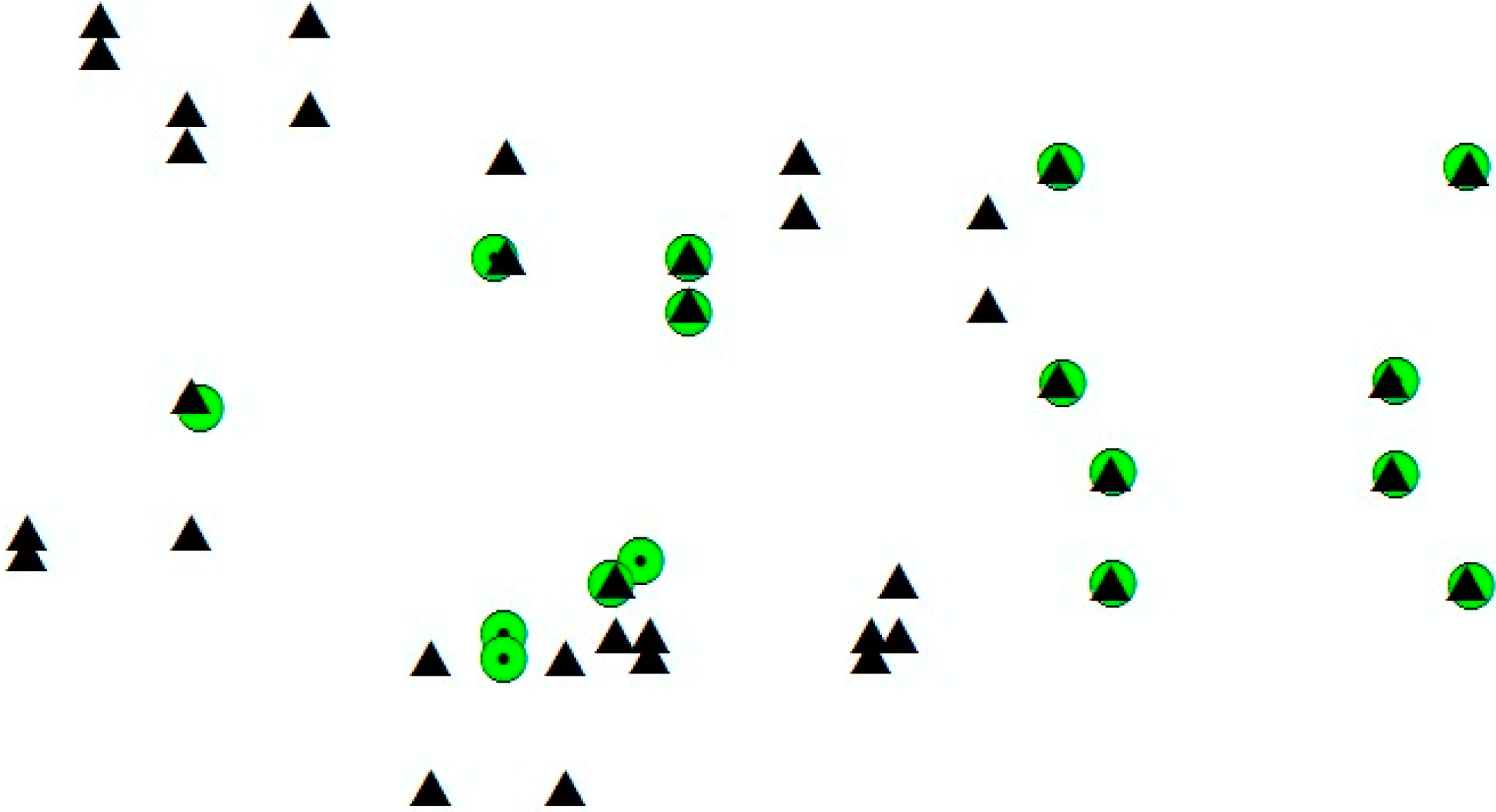
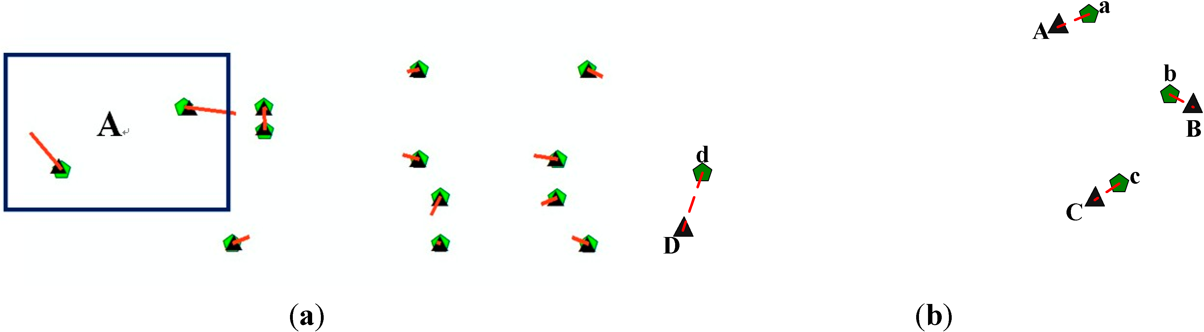
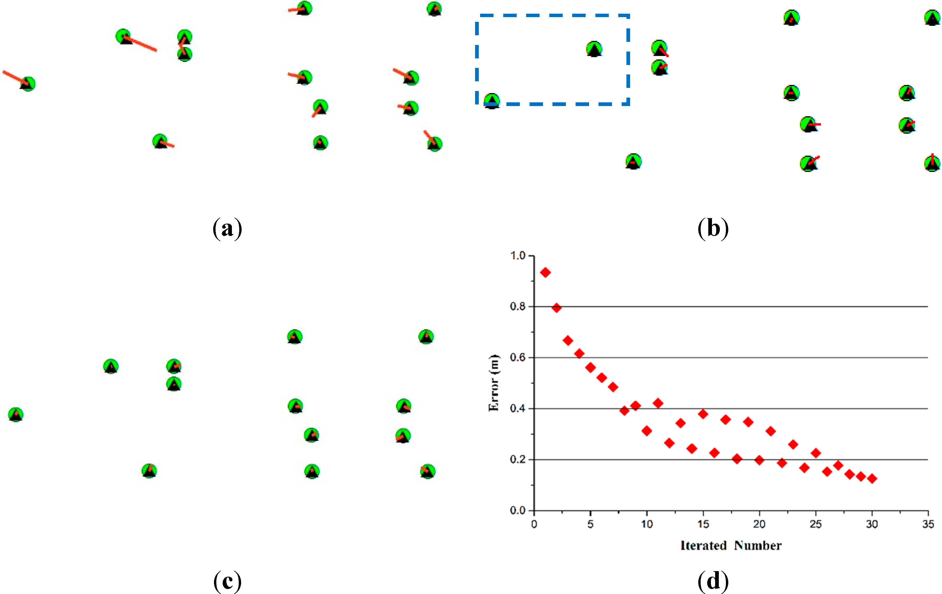
The initial matching of corners is obtained after all points in B have been converted by resorting to the best transformation matrix R1 and T1 (Figure 2; green circles are terrestrial corners, and black triangles are airborne corners).
Figure 2. Initial matching results of airborne corners (black triangles) and terrestrial corners (green circles).
Remotesensing 07 01915 g002

3.3. Shiftable Leading Point Method for Improvement of the Geometric Accuracy of Registration

As mentioned in the Introduction, the extracted airborne corners are usually of low geometric accuracy and include numerous anomalous corners, as shown in Figure 3a, in which two anomalous corners are seen in region A. When the least squares method is used for the determination of the transformation matrix, the relatively large errors of anomalous corners will be magnified to affect the whole dataset, resulting in a global deviation of the registered data. A usual way to deal with these situations with anomalous data is to utilize the RANSAC algorithm, which searches for inliers to determine the models. However, due to the limited scanning range of terrestrial LiDAR, few corners can be extracted, offering few conjugate features. For example, in our experiment, terrestrial LiDAR data are scanned from nine stations, which cover 250 m × 100 m. Only 16 building corners are extracted and 13 conjugate features are obtained. As the registration accuracy is influenced by the amount, distribution and geometric accuracy of conjugate features. When faced with few conjugate features, it is not fit to filter the features for the inliers, e.g., the RANSAC algorithm, which may do great harm to the distribution of original features. In Figure 3b, if the RANSAC algorithm is used, point d will be recognized as an outlier and not be used for the registration. When only points a, b and c are used for the registration, as they are locally and densely distributed, the transformation matrix may fit the local area around points a, b and c well; nevertheless, when the distance from this local area increases, the registration error will be enlarged. When the distance reaches a certain degree, the error caused with distance increasing will be larger than that of point d. Actually, the differences between the errors of corners are extremely small compared with the distances between corners. In this way, in spite of the relatively large deviation of point d, it can offer its contribution to the registration.
In this paper, a shiftable leading point method is proposed. As shown in Figure 4a–d is terrestrial corners; A, B, C and D are airborne corners, among which, D is an anomalous corner. After the least squares method for the registration matrix, the registration result is shown in Figure 4b. As we can see, an obvious deviation is seen between D and d, with small deviations between the other conjugate points. It is easy to know that due to the large deviation of the anomalous point, its deviation is also allocated to other points, resulting in an increase in global deviation. To address this problem, a usual way is to abandon this point pair; nevertheless, in some situations, this point can also contribute to the registration as before. In our method, leading points are generated from airborne corners as A’, B’, C’ and D’ in Figure 4c. As for the leading point with the largest error (D’ in Figure 4c), it is shifted to its corresponding terrestrial corner, as shown in Figure 4d. Note that during this procedure, only one leading point is shifted, and the airborne corners are unchanged. After that, A’, B’, C’ and D’ are used to register with a, b, c, and d, and the result is shown in Figure 4e. Then, the registration matrix from the leading points and terrestrial corners is used to transform airborne corners and airborne LiDAR points, as shown in Figure 4f. In Figure 4f, A, B and C match much better with a, b, and c than in Figure 4b. The global deviation caused by the anomalous corner is eliminated effectively. Apart from that, due to the existence of point pair D and D’, the overall distribution of point pairs is also retained. The registration error caused by the destroying of the distribution of conjugate features is not seen in this method.
Figure 3. Basis for the shiftable leading point method. (a) Example of extracted airborne corners (green pentagons refer to true airborne corners; black triangles refer to airborne corners; red straight lines refer to error vectors, which are amplified 10 times); (b) example of unevenly distributed corners (green pentagons refer to true airborne corners; black triangles refer to airborne corners).
Remotesensing 07 01915 g003
Additionally, a criterion is required to halt the iteration process in this method. The registration accuracy of leading points and terrestrial corners is obviously enhanced after the first shifting (Figure 4f). When leading points with relatively large deviation exist, the global accuracy between conjugate points is always enhanced after iteration, maintaining the continual reduction of errors (Figure 4g). However, the registration error begins to fluctuate after several iterations. This is intuitive: there are no leading points with obvious deviation, i.e., the position errors of conjugate points are approximately equal, such that the movement of any point could results in inappropriate movement from the correct position to a wrong position. In this situation, the positions of many accurate points may deviate, even if the resulting position error has been diminished to zero by iterations. Accordingly, the total minimum error between conjugate points cannot be applied as the criterion to halt iteration: the iteration processes stop when the overall error of conjugate points starts to fluctuate. Here, a comparison of the overall error of conjugate points is conducted between two consecutive iterations. If the current error is several times larger than the former one, the iteration stops. The threshold here is usually set between 1–1.5 because the fluctuation is usually not very prominent. After the iteration procedure, the final transformation matrix is used to register the airborne and terrestrial LiDAR points.
Figure 4. A shiftable leading point method (airborne corners: red circles; terrestrial corners: green circles; leading point: yellow triangles). (a) Original airborne and terrestrial corners; (b) airborne and terrestrial corners after registration; (c) generated leading points from airborne corners; (d) shift of a leading point; (e) registration of leading points and terrestrial corners; (f) transformation of airborne corners with the registration matrix in (e); (g) change of the geometric error of leading points and terrestrial corners with iterations.
Remotesensing 07 01915 g004
The airborne corners are set as P = {Pi, i = 0, 1, 2, …, n} and the terrestrial corners as U = {Ui, i = 0, 1, 2, …, n}. The shiftable leading point method operates as follows.
(1)
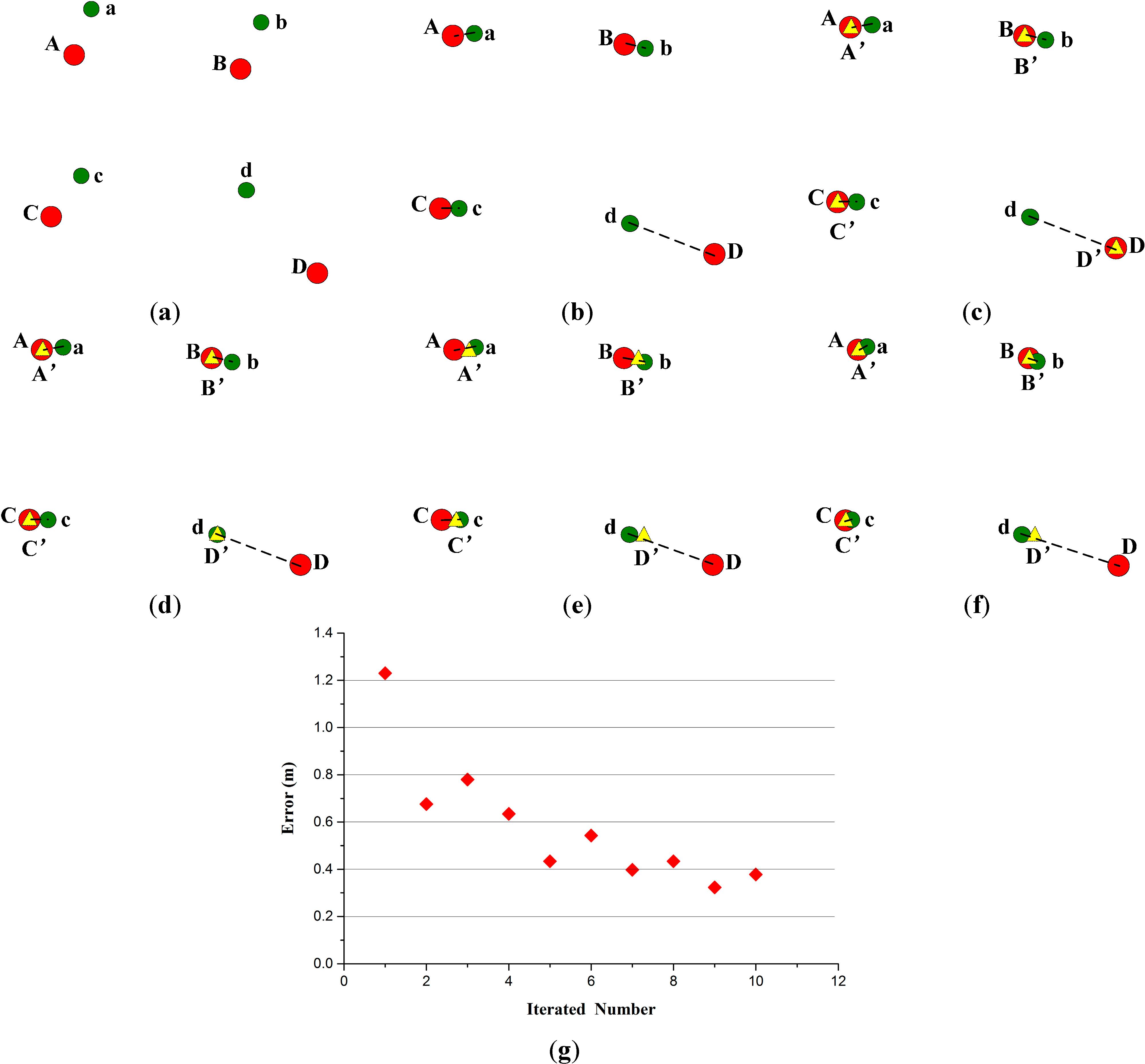
Register P and U using the least squares algorithm, and obtain a rotation matrix R and a translation matrix T, with which the airborne corners P are transformed as Q = {Qi, i = 0, 1, 2, …, n} (there is no leading point shift in the first iteration).
(2)
Calculate the three-dimensional spatial distance between conjugate points among point set P and its corresponding point set U, and obtain a one-dimensional distance matrix D = {D(Ui,Qi), i = 0, 1, 2, … n}. Calculate the overall position error of conjugate points E r r = i = 1 n D i ; the iteration is stopped if Errcurrent > thresh × Errpre , where Errcurrent is the current position error, thre is a threshold and Errpre is the former position error.
(3)
Seek the maximum distance in D and find its corresponding points Umax and Qmax in point sets U and Q, respectively. Shift leading point Qmax to the corresponding terrestrial corner Umax. Point set P is modified as P = {P1, P2, …, Pmax, …, Pn}.
(4)
Repeat procedures (1)–(3) until the iteration stops during Procedure (2). The final transformation matrix is used to register airborne and terrestrial LiDAR points, thus finishing the registration procedure.

4. Experiment and Analysis

4.1. Experimental Data

The campus of Nanjing University, China, which covers an area of about 400 m × 1600 m, is selected as the experimental area. The airborne and terrestrial LiDAR data for this area are presented in Figure 5. The average point spacing of airborne LiDAR data is 1.0 m, with a vertical error of 0.2 m and a horizontal error of 0.3 m; the dataset has around 460,000 points in total. Terrestrial LiDAR data are obtained using the Leica Scanstation 2 scanner, with a planar accuracy of 6 mm, a vertical accuracy of 4 mm and an average point spacing of 10 cm, at a range of 50 m. Terrestrial LiDAR points collected by nine survey stations are registered manually based on targets to form the dataset in Figure 5b, resulting in about 30 million points.
Figure 5. Experimental data. (a) Airborne LiDAR data; (b) terrestrial LiDAR data (collected by nine terrestrial survey stations manually registered based on targets).
Remotesensing 07 01915 g005

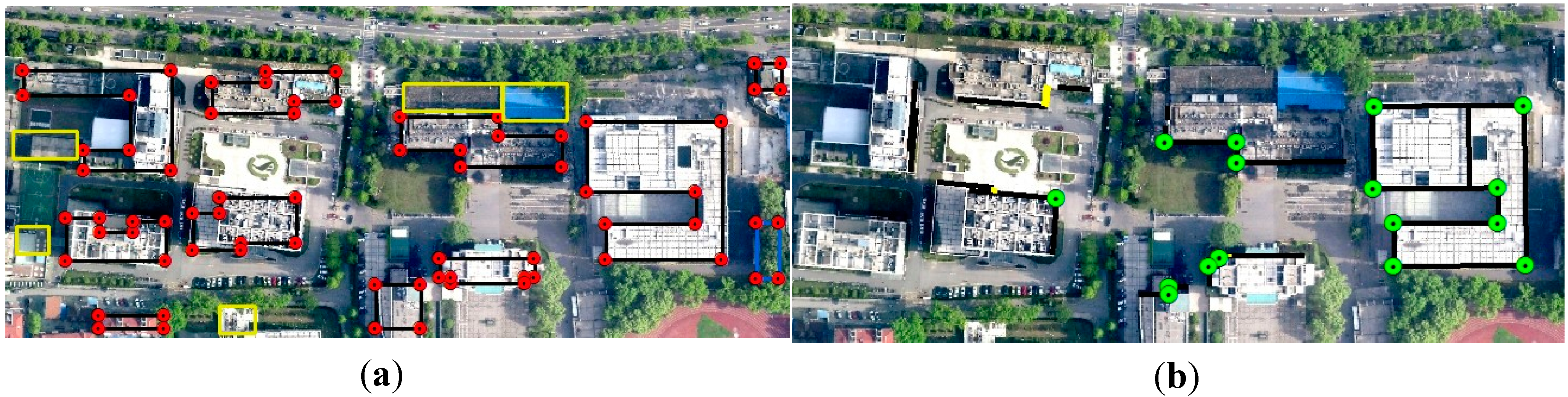
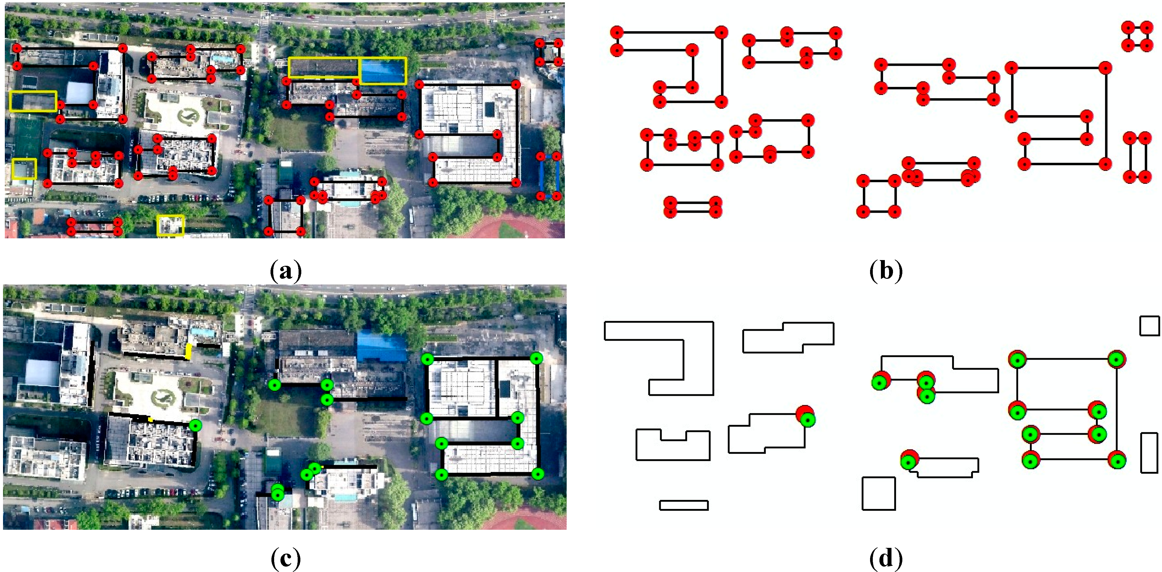
4.2. Evaluation of Building Contour and Corner Extraction

Building contours and corners are extracted from airborne LiDAR data using the RIMM and a regularization method. According to the RIMM [47], the relevant thresholds are set as follows: The maximum window size threshold (106 m) and minimum window size threshold (6 m) are assigned according to the maximum and minimum of the building sizes in this study, respectively. The height value of this lowest building is taken as the height difference threshold (15 m in this study). For the threshold of step length, it should be set as small as possible, because only a small threshold can eliminate the influences of high-relief terrain in iteration processes. In general, the step length value cannot be larger than the height difference threshold. On the other hand, too intensive iterations would reduce the efficiency of the processes. To keep the balance of the two aspects, the step length threshold is determined as 10 m in this study. The roughness value (1.6 in this study), which is the mean square deviation of the elevations of the points in a rectangle window (with a size of 6 m), is set empirically to separate the building points and tree points. Building contours and corners are obtained from LiDAR data, shown in Figure 6a. In this figure, the black segments are those contours correctly extracted, with the blue ones falsely extracted. The yellow ones are the missing extracted ones. Correctness and completeness are used as two indexes to evaluate the contours, and the formula is as follows:
C o m p l e t e n e s s = T P T P + F N C o r r e c t n e s s = T P T P + F P
In the formula, TP refers to the number of correctly extracted contours, FN is the number of missing contours and FP is the number of incorrect contours.
As shown in Table 1, the correctness and completeness of extracted airborne building contours are 95.2% and 79.8%, respectively. As we can see, the extracted building contours bear high correctness, which can benefit the registration using building contours due to the small noise. As for the extracted contours, 72 corners are finally obtained as shown in Figure 6b.
Table 1. Evaluation of the correctness and completeness of building contours.
Actual NumberCorrect NumberIncorrect NumberMissing NumberCorrectnessCompleteness
Airborne contours997942095.2%79.8%
Terrestrial contours363303100%91.7%
The DoPP method is used to extract building contours and corners from terrestrial LiDAR data [49]. Through the quantitative estimation, the density threshold is estimated to be 389, based on the following parameters: the farthest building from the scanner is 50 m away; the height of the building is 40 m; the height of the equipment is 1.5 m; the minimum horizontal distance is 25 m; and the ratio of window-to-wall is set as 0.5. Figure 6c presents the extracted terrestrial building contours and corners. In this figure, the black segments are those contours correctly extracted and the yellow ones are those missing extracted ones. As shown in Table 1, the correctness and completeness of terrestrial building contours are 100% and 91.7%, respectively, both of which are quite high. A total of 16 corners are finally extracted from terrestrial building contours.
MTMM is conducted for airborne and terrestrial corners after the extraction of two types of corners, in which the matching distance threshold is set as 5 m. Thirteen pairs of conjugate corners are obtained (Figure 6d). True building corners are digitized from an orthophoto for the geometric accuracy of conjugate corners, and their elevations are set by averaging the points near the building contours. As shown in Table 2, the average error, maximum error and RMSE of these airborne corners are 0.91 m, 2.15 m and 1.08 m. The average error, maximum error and RMSE of these terrestrial corners are 0.13 m, 0.19 m and 0.14 m, respectively; this represents much higher geometric accuracy than that of airborne corners.
Figure 6. Building corner extraction from airborne and terrestrial LiDAR data. (a) Evaluation of extracted building contours from airborne LiDAR data; (b) extracted airborne corners; (c) evaluation of extracted building contours from terrestrial LiDAR data; (d) initial registration results of airborne corners and terrestrial corners.
Remotesensing 07 01915 g006
Table 2. Evaluation of the geometric precision of conjugate building corners.
Average Error (m)Max Error (m)RMSE (m)
Airborne corners0.912.151.08
Terrestrial corners0.130.190.14

4.3. Change of Error between Leading and Terrestrial Point Pairs during Iterations

After the matching of airborne and terrestrial corners, leading points are generated from airborne corners, and the shifted leading point method is conducted. To test the effect of the proposed shiftable leading point method, comparative experiments are designed using three approaches: fixed corner (FC, without the shiftable leading point), RANSAC (RC, remove outlier conjugate points) and shiftable corner (SC, with the shiftable leading point).
The distance between conjugate points can be calculated in each iteration of the leading point shift process. Using FC, the geometric errors of leading points and terrestrial corners are shown in Figure 7a, where green circles represent the terrestrial corners after the first iteration, black triangles represent leading points (no leading point shift in this step) and red lines represent error vectors (amplified 10 times). It is clear that the lengths of error vectors vary considerably, and many are extremely long. Table 3 presents a quantitative assessment of the errors, with an average error of 0.93 m, a maximum error of 1.94 m and an RMSE of 1.06 m. The average error between leading points and terrestrial corners using FC still reaches up to 0.93 m, with some values even approaching 2 m; this could lead to unacceptably large errors in the final registration result.
Figure 7. Geometric error of leading points and referenced points. (a) Geometric error of leading points (black triangles) and referenced points (green circles) by using FC (fixed corner, without the shiftable leading point) (red lines represent error vectors, which are amplified 10 times); (b) geometric error of leading points (black triangles) and referenced points (green circles) by using RC (RANSAC; removed points in the box); (c) geometric error of leading points and referenced points by using SC (shifted corner, with the shiftable leading point), after the 10th iteration; (d) change of the geometric error of leading points and referenced points with iterations by using SC.
Remotesensing 07 01915 g007
Table 3. Evaluation of the geometric precision of leading points and referenced points.
Average Error (m)Max Error (m)RMSE (m)
FC0.931.941.06
RC0.611.300.41
SC0.310.510.34
Compared with FC, the outlier conjugate points (points in the blue box of Figure 7b) have been removed in RC. Using RC, the geometric errors of leading points and terrestrial corners are shown in Figure 7b, from which it can be seen that the error vectors are shorter than the error vectors in Figure 7a. However, the lengths of part error vectors are still long, which could lead to some errors in the final registration result. The average error, maximum error and RMSE are 0.61 m, 1.30 m and 0.41 m, respectively (Table 3).
Using SC, after ten iterations (nine point shifts), geometric position errors between the leading points and terrestrial corners are as shown in Figure 7c, from which it can be seen that the error vectors are shorter and approximately the same length. The average error, maximum error and RMSE are 0.31 m, 0.51 m and 0.34 m, respectively (Table 3). Compared with the results presented in Figure 7a,b, the geometric position errors of leading points and terrestrial corners are reduced obviously. This study calculates the geometric errors of conjugate points from Iterations 1–30 (Figure 7d). There is a clear decline in errors during Iterations 1–10, but the error starts to fluctuate and declines slowly from Iteration 10 onward. Therefore, it is correct and feasible that the criterion for halting iteration is determined as the point at which error fluctuation begins to occur.

4.4. Evaluation of Geometric Accuracy of LiDAR Data Registration
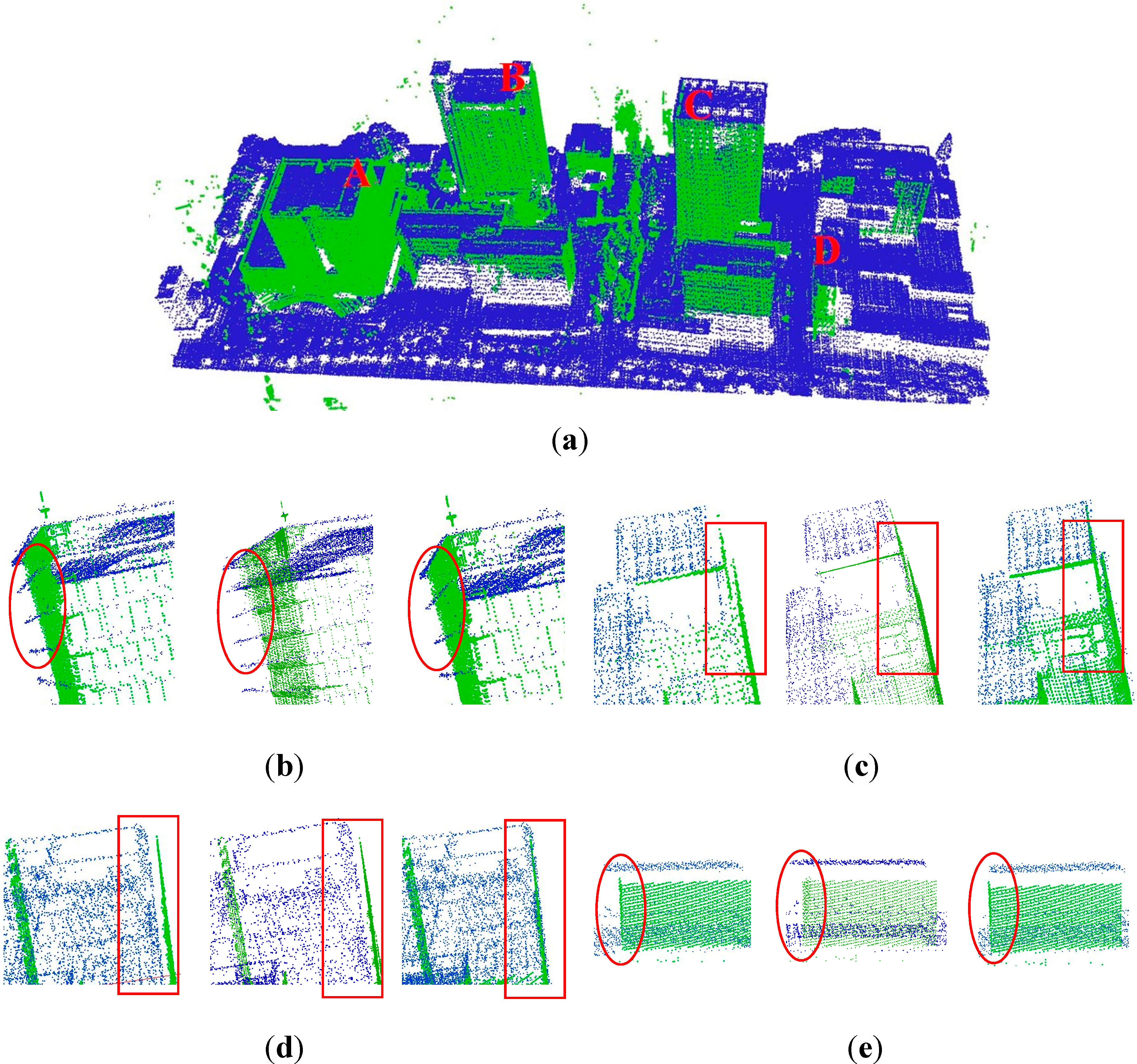
4.4.1. Visual Check

Figure 8a presents the result of the registration of airborne and terrestrial LiDAR data by using SC. Overall, it is clear that airborne and terrestrial LiDAR data match well. Figure 8b illustrates partial enlarged drawings of A by using FC, RC and SC. Similarly, Figure 8c–e are partial enlarged drawings of B, C and D, respectively, in the registration results of FC, RC and SC. Red circles and boxes in Figure 8b–e indicate obvious differences between the two registration results of LiDAR data, e.g., the apparent deviation of the wall in B and C, the rightward deviation in D. A comparison indicates that matching with the shiftable leading point method improves the quality of the registration of airborne and terrestrial LiDAR data and simultaneously results in higher geometric accuracy.
Figure 8. Comparison of the registration of airborne and terrestrial LiDAR data. (a) Registration results by using SC; (be) differences of Labels A, B, C and D, respectively.
Remotesensing 07 01915 g008

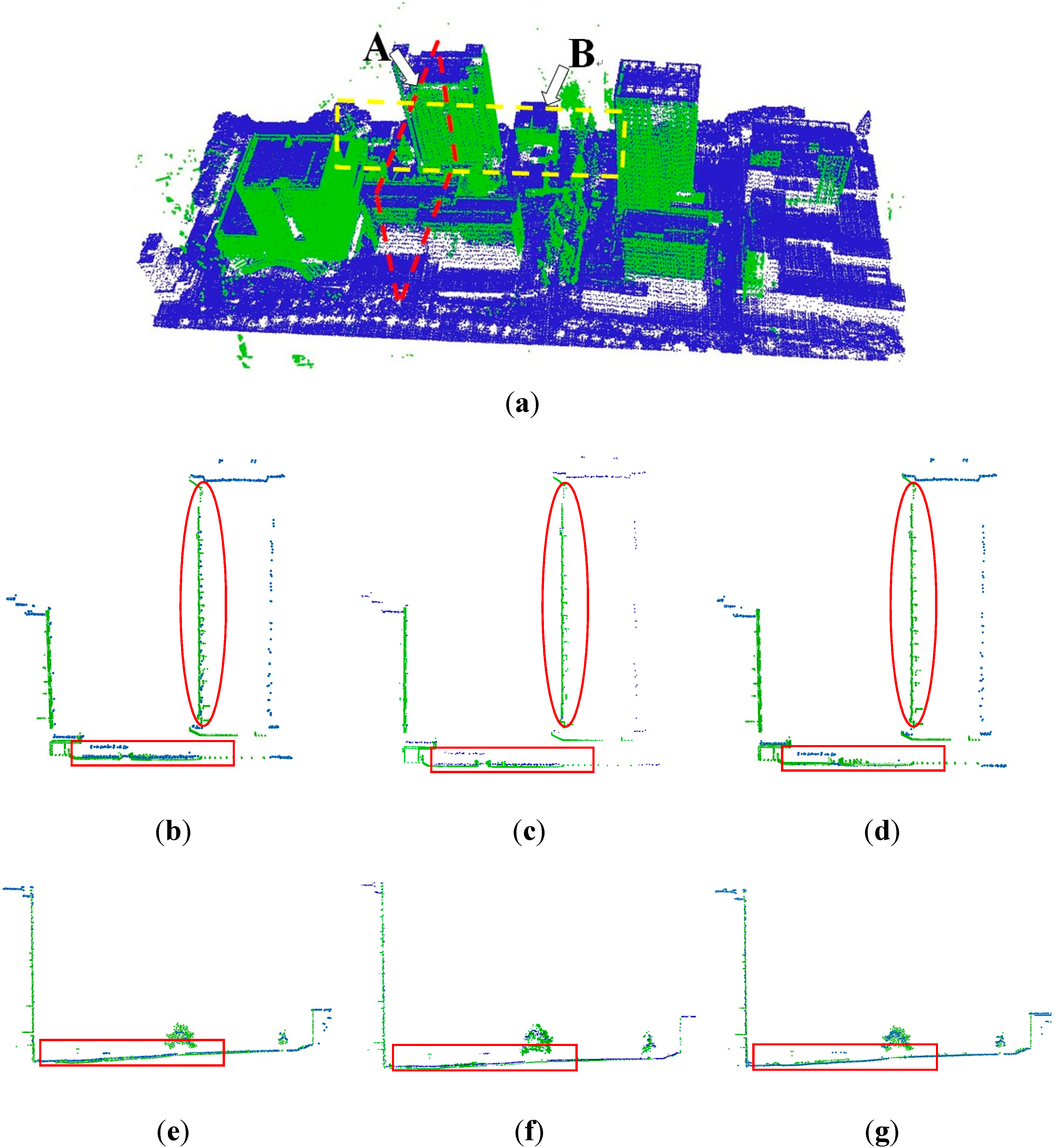
4.4.2. Evaluation with Common Sections

Figure 9 presents an evaluation of the registration result using FC, RC and SC with common sections. Figure 9a illustrates the positions of two sections. Section A is oriented south and north, with section B east and west. Figure 9b–d is the details of section A using FC, RC and SC respectively. Red circles in Figure 9b show the obvious deviation of the walls using FC, while in Figure 9d, no deviation is seen. This shows that the shiftable leading point method can improve the registration accuracy of airborne and terrestrial LiDAR data in the horizontal direction. Meanwhile, the red box near the ground area in Figure 9b shows more serious deviation than that in Figure 9d and similar situations are seen in Figure 9e–g. A conclusion can be drawn as the shiftable leading point method can also improve the registration of airborne and terrestrial LiDAR data in the vertical direction.
Figure 9. Evaluation with common sections. (a) Positions of the sections; (b) section A by using FC; (c) section A by using RC; (d) section A by using SC; (e) section B by using FC; (f) section B by using RC; (g) section B by using SC.
Remotesensing 07 01915 g009

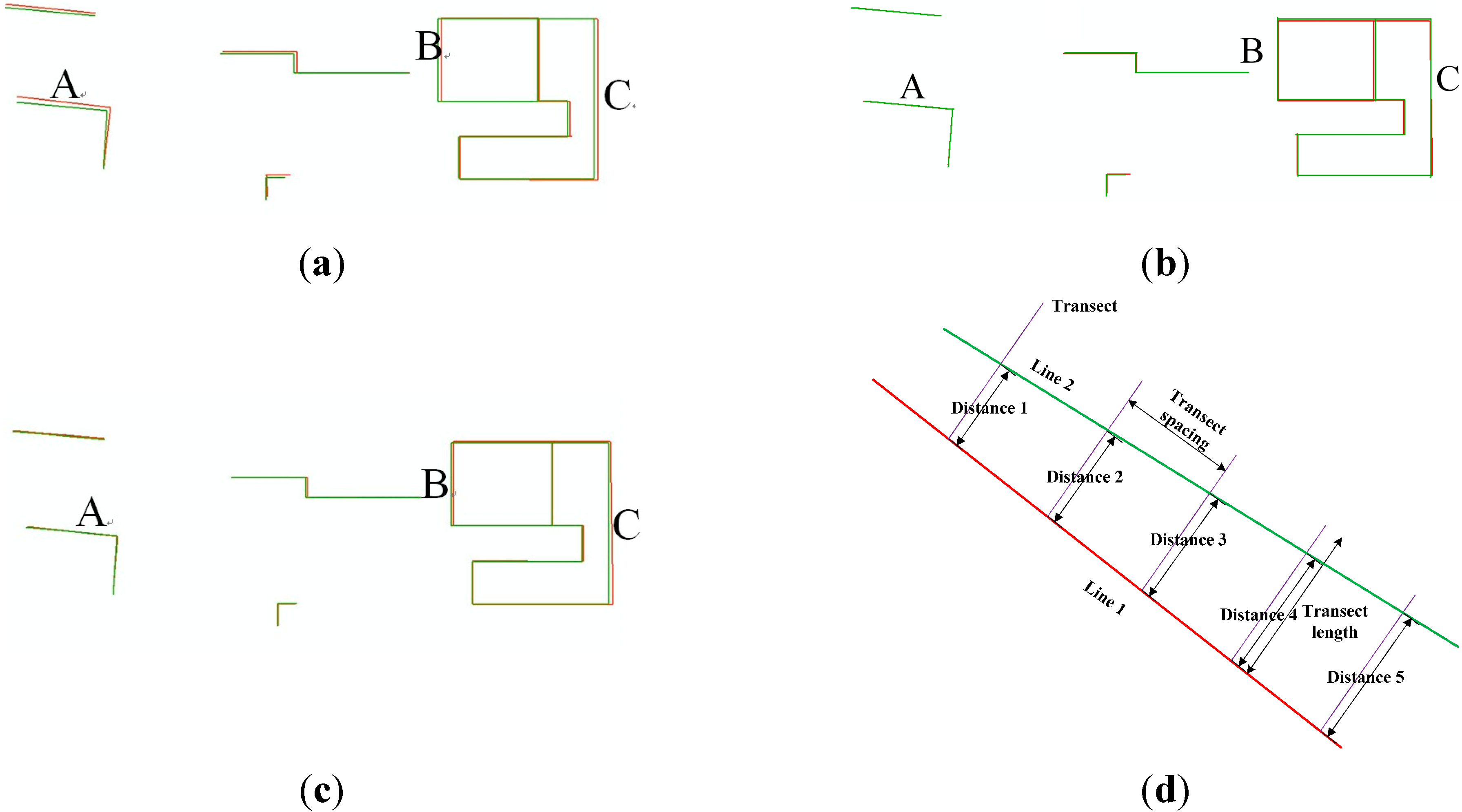
4.4.3. Quantitative Analysis using Common Building Contours

An evaluation is conducted using 2D building contour lines, which are extracted manually from registered airborne and terrestrial LiDAR. Figure 10a–c illustrates the registration results for the digitized conjugate contour lines, in which the green and red lines represent building contours derived from airborne and terrestrial LiDAR data, respectively. A comparison of these figures indicates that the overlaying situation of the common building contours varies depending on whether the proposed method is used. It is clear that the distances between conjugate contour lines in Figure 10a,b are larger than those of Figure 10c, particular in A, B and C.
The transect distance and angles between conjugate contour lines are calculated to conduct a quantitative assessment of these registration results. The method for calculating transect distance is illustrated in Figure 10d. One contour is taken as a baseline, and lines perpendicular to this baseline are constructed at a specified interval; the distance between the baseline and corresponding contour is the transect distance. The average transect distance between two conjugate contours is the distance between two contours. The average distance, maximum distance and RMSE calculated using FC are 0.81 m, 1.73 m and 0.95 m, respectively (Table 4); those calculated using RC are 0.49 m, 0.96 m and 0.38 m, respectively; those calculated using SC are 0.31 m, 0.89 m and 0.37 m, respectively. Meanwhile, the average angle error, maximum error and RMSE calculated using FC are 0.75°, 2.80° and 0.95°, respectively; those calculated using SC are 0.71°, 1.89° and 0.60°; those calculated using SC are 0.44°, 1.30° and 0.53°. Errors in both the transect distance and angle are effectively reduced.
Figure 10. Geometric precision evaluation by using common building boundaries. (a) The registered boundaries from airborne (red) and terrestrial (green) LiDAR data by using FC; (b) the registered boundaries from airborne and terrestrial LiDAR data by using RC; (c) the registered boundaries from airborne and terrestrial LiDAR data by using SC; (d) length of transect lines.
Remotesensing 07 01915 g010
Table 4. Evaluation of the geometric precision of LiDAR data registration using building boundaries.
Transect Distance (m)Angle (Degree)
ErrorAverageMaxRMSEAverageMaxRMSE
FC0.811.730.950.752.800.95
RC0.490.960.380.711.890.60
SC0.310.890.370.441.300.53

4.4.4. Quantitative Analysis using Common Ground Points

As the evaluation with 2D building contours is just done for the horizontal accuracy, a further evaluation for the vertical accuracy is done with common ground points. Twenty five sample points are randomly selected in their common ground region to compare the height difference between the interpolation results of airborne and terrestrial LiDAR data. As shown in Table 5, the average distance, max distance and RMSE of the sample points using FC are 0.51 m, 0.82 m and 0.56 m, respectively; those calculated using RC are 0.43 m, 0.62 m and 0.38 m; those calculated using SC are 0.26 m, 0.46 m and 0.30 m. The distances between the common ground points are reduced effectively. Thus, the proposed shiftable leading point method can effectively advance the registration accuracy of terrestrial and airborne LiDAR data.
Table 5. Evaluation of the geometric precision of LiDAR data registration using common ground points.
AverageMaxRMSE
FC0.510.820.56
RC0.430.620.38
SC0.260.460.30

5. Conclusions

A new approach based on a shiftable leading point method is proposed for improving the registration of airborne and terrestrial LiDAR data. The following conclusions are reached based on the experiment and analysis. The DoPP method with quantitative threshold estimation can effectively extract building corners with high geometric accuracy. The shiftable leading point method can effectively modify the leading points with relatively large errors, in which the iterative strategy ensures the correctness of point moving without disrupting the stability of points. Iteration that terminates according to the fluctuation of geometric error between leading points and terrestrial corners can ensure the global accuracy of conjugate points and control the computation amount to the greatest extent. The proposed shiftable leading point method, which effectively addresses the impact caused by the uneven distribution of terrestrial corners, can lead to high accuracy in the registration of airborne and terrestrial LiDAR data. However, if the terrestrial building corners are sufficient and distributed uniformly in the registration region, the proposed shiftable points method would have almost the same effect as the RANSAC-type methods (e.g., removing of poor matching corners).
In addition, this study has certain limitations. Firstly, this method has difficulty dealing with non-urban regions, which contain almost no geometric buildings. Besides, it is still difficult to achieve ideal results for the registration of those buildings with eaves. If the buildings have eaves, there is a deviation between the building contours extracted from the airborne and terrestrial LiDAR data. The deviation is determined by the size of the building eaves. As a result, few corresponding corners can be extracted, and the registration result is not ideal. Therefore, we will perform a further study on eaves by using the center point of the building convex hull or other auxiliary data.

Acknowledgments

This work is supported by the National Natural Science Foundation of China (Grant No. 41371017, 41001238) and the National Key Technology R&D Program of China (Grant No. 2012BAH28B02). Sincere thanks are given for the comments and contributions of the anonymous reviewers and members of the editorial team.

Author Contributions

Liang Cheng proposes the core idea of shiftable leading point method and designs the technical framework of the paper. Lihua Tong implements the registration method of shiftable leading point. Yang Wu implements the method of extraction of building corners from airborne and terrestrial LiDAR data. Yanming Chen is responsible for the implementation of the comparative experiments. Manchun Li is responsible for experimental analysis and discussion.

Conflicts of Interest

The authors declare no conflict of interest.

References

  1. Bang, K.I.; Habib, A.F.; Kusevic, K.; Mrstik, P. Integration of terrestrial and airborne LiDAR data for system calibration. In Proceedings of the International Archives of the Photogrammetry, Remote Sensing and Spatial Information Sciences, Beijing, China, 3–11 July 2008; pp. 391–398.
  2. Chen, Y.; Cheng, L.; Li, M.; Wang, J.; Tong, L.; Yang, K. Multiscale grid method for detection and reconstruction of building roofs from airborne LiDAR data. IEEE J. Sel. Top. Appl. Earth Obs. Remote Sens. 2014, 7, 4081–4094. [Google Scholar] [CrossRef]
  3. Cheng, L.; Wu, Y.; Wang, Y.; Zhong, L.; Chen, Y.; Li, M. Three-Dimensional reconstruction of large multilayer interchange bridge using airborne LiDAR data. IEEE J. Sel. Top. Appl. Earth Obs. Remote Sens. 2014, 8. [Google Scholar] [CrossRef]
  4. Cheng, L.; Tong, L.; Wang, Y.; Li, M. Extraction of urban power lines from vehicle-borne LiDAR data. Remote Sens. 2014, 6, 3302–3320. [Google Scholar] [CrossRef]
  5. Puttonen, E.; Lehtomäki, M.; Kaartinen, H.; Zhu, L.; Kukko, A.; Jaakkola, A. Improved sampling for terrestrial and mobile laser scanner point cloud data. Remote Sens. 2013, 5, 1754–1773. [Google Scholar] [CrossRef]
  6. Eysn, L.; Pfeifer, N.; Ressl, C.; Hollaus, M.; Grafl, A.; Morsdorf, F. A practical approach for extracting tree models in forest environments based on equirectangular projections of terrestrial laser scans. Remote Sens. 2013, 5, 5424–5448. [Google Scholar] [CrossRef]
  7. Kang, Z.; Zhang, L.; Tuo, L.; Wang, B.; Chen, J. Continuous extraction of subway tunnel cross sections based on terrestrial point clouds. Remote Sens. 2014, 6, 857–879. [Google Scholar] [CrossRef]
  8. Weinmann, M.; Weinmann, M.; Hinz, S.; Jutzi, B. Fast and automatic image-based registration of TLS data. ISPRS J. Photogramm. Remote Sens. 2011, 66, S62–S70. [Google Scholar] [CrossRef]
  9. Heritage, G.; Large, A. Laser Scanning for the Environmental Sciences; Wiley-Blackwell: Hoboken, NJ, USA, 2009. [Google Scholar]
  10. Ruiz, A.; Kornus, W.; Talaya, J.; Colomer, J.L. Terrain modeling in an extremely steep mountain: A combination of airborne and terrestrial LiDAR. In Proceedings of the 20th International Society for Photogrammetry and Remote Sensing (ISPRS) Congress on Geo-imagery Bridging Continents, Istanbul, Turkey, 12–23 July 2004; pp. 1–4.
  11. Heckmann, T.; Bimböse, M.; Krautblatter, M.; Haas, F.; Becht, M.; Morche, D. From geotechnical analysis to quantification and modelling using LiDAR data: A study on rockfall in the Reintal catchment, Bavarian Alps, Germany. Earth Surf. Process. Landforms 2012, 37, 119–133. [Google Scholar] [CrossRef]
  12. Jung, S.E.; Kwak, D.A.; Park, T.; Lee, W.K.; Yoo, S. Estimating crown variables of individual trees using airborne and terrestrial laser scanners. Remote Sens. 2011, 3, 2346–2363. [Google Scholar] [CrossRef]
  13. Hohenthal, J.; Alho, P.; Hyyppä, J.; Hyyppä, H. Laser scanning applications in fluvial studies. Prog. Phys. Geog. 2011, 35, 782–809. [Google Scholar] [CrossRef]
  14. Kedzierski, M.; Fryskowska, A. Terrestrial and aerial laser scanning data integration using wavelet analysis for the purpose of 3D building modeling. Sensors 2014, 14, 12070–12092. [Google Scholar] [CrossRef] [PubMed]
  15. Jaw, J.J.; Chuang, T.Y. Feature-based registration of terrestrial and aerial LiDAR point clouds towards complete 3D scene. In Proceedings of the 29th Asian Conference on Remote Sensing, Colombo, Sri Lanka, 10–14 November 2008; pp. 10–14.
  16. Fischler, M.A.; Bolles, R.C. Random sample consensus: A paradigm for model fitting with applications to image analysis and automated cartography. Commun. ACM 1981, 24, 381–395. [Google Scholar] [CrossRef]
  17. Hilker, T.; Coops, N.C.; Culvenor, D.S.; Newnham, G.; Wulder, M.A.; Bater, C.W.; Siggins, A. A simple technique for co-registration of terrestrial LiDAR observations for forestry applications. Remote Sens. Lett. 2012, 3, 239–247. [Google Scholar] [CrossRef]
  18. Liang, X.H.; Liang, J.; Xiao, Z.Z.; Liu, J.W.; Guo, C. Study on multi-views point clouds registration. Adv. Sci. Lett. 2011, 4, 8–10. [Google Scholar]
  19. Wang, J. Block-to-Point fine registration in terrestrial laser scanning. Remote Sens. 2013, 5, 6921–6937. [Google Scholar] [CrossRef]
  20. Jaw, J.J.; Chuang, T.Y. Registration of ground-based LiDAR point clouds by means of 3D line features. J. Chin. Inst. Eng. 2008, 31, 1031–1045. [Google Scholar] [CrossRef]
  21. Bucksch, A.; Khoshelham, K. Localized registration of point clouds of botanic Trees. IEEE Geosci. Remote Sens. Lett. 2013, 10, 631–635. [Google Scholar] [CrossRef]
  22. Von Hansen, W. Robust automatic marker-free registration of terrestrial scan data. Proc. Photogramm. Comput. Vis. 2006, 36, 105–110. [Google Scholar]
  23. Stamos, I.; Leordeanu, M. Automated feature-based range registration of urban scenes of large scale. In Proceedings of the 2003 IEEE Computer Society Conference on Computer Vision and Pattern Recognition, New York, NY, USA, 18–20 June 2003; pp. II-555–Ii-561.
  24. Zhang, D.; Huang, T.; Li, G.; Jiang, M. Robust algorithm for registration of building point clouds using planar patches. J. Surv. Eng. 2011, 138, 31–36. [Google Scholar] [CrossRef]
  25. Bae, K.H.; Lichti, D.D. A method for automated registration of unorganised point clouds. ISPRS J. Photogramm. Remote Sens. 2008, 63, 36–54. [Google Scholar] [CrossRef]
  26. Chen, H.; Bhanu, B. 3D free-form object recognition in range images using local surface patches. Pattern Recognit. Lett. 2007, 28, 1252–1262. [Google Scholar] [CrossRef]
  27. He, B.; Lin, Z.; Li, Y.F. An automatic registration algorithm for the scattered point clouds based on the curvature feature. Opt. Laser Technol. 2012, 46, 53–60. [Google Scholar] [CrossRef]
  28. Makadia, A.; Patterson, A.; Daniilidis, K. Fully automatic registration of 3D point clouds. In Proceedings of the 2006 IEEE Computer Society Conference on Computer Vision and Pattern Recognition, New York, NY, USA, 17–22 June 2006; pp. 1297–1304.
  29. Han, J.Y.; Perng, N.H.; Chen, H.J. LiDAR point cloud registration by image detection technique. IEEE Geosci. Remote Sens. Lett. 2013, 10, 746–750. [Google Scholar] [CrossRef]
  30. Al-Manasir, K.; Fraser, C.S. Registration of terrestrial laser scanner data using imagery. Photogramm. Rec. 2006, 21, 255–268. [Google Scholar] [CrossRef]
  31. Akca, D. Matching of 3D surfaces and their intensities. ISPRS J. Photogramm. Remote Sens. 2007, 62, 112–121. [Google Scholar] [CrossRef]
  32. Wang, Z.; Brenner, C. Point based registration of terrestrial laser data using intensity and geometry features. In Proceedings of the International Archives of Photogrammetry, Remote Sensing and Spatial Information Sciences, Beijing, China, 3–11 July 2008; pp. 583–589.
  33. Kang, Z.; Li, J.; Zhang, L.; Zhao, Q.; Zlatanova, S. Automatic registration of terrestrial laser scanning point clouds using panoramic reflectance images. Sensors 2009, 9, 2621–2646. [Google Scholar] [CrossRef] [PubMed]
  34. Eo, Y.D.; Pyeon, M.W.; Kim, S.W.; Kim, J.R.; Han, D.Y. Coregistration of terrestrial LiDAR points by adaptive scale-invariant feature transformation with constrained geometry. Autom. Constr. 2012, 25, 49–58. [Google Scholar] [CrossRef]
  35. Schenk, T.; Krupnik, A.; Postolov, Y. Comparative study of surface matching algorithms. Int. Arch. Photogramm. Remote Sens. 2000, 33, 518–524. [Google Scholar]
  36. Maas, H.G. Least-Squares matching with airborne laser scanning data in a TIN structure. Int. Arch. Photogramm. Remote Sens. 2000, 33, 548–555. [Google Scholar]
  37. Bretar, F.; Pierrot-Deseilligny, M.; Roux, M. Solving the strip adjustment problem of 3D airborne lidar data. In Proceedings of Geoscience and Remote Sensing Symposium, Anchorage, AK, USA, 20–24 September 2004; pp. 4734–4737.
  38. Lee, J.; Yu, K.; Kim, Y.; Habib, A.F. Adjustment of discrepancies between LiDAR data strips using linear features. IEEE Geosci. Remote Sens. Lett. 2007, 4, 475–479. [Google Scholar] [CrossRef]
  39. Habib, A.F.; Kersting, A.P.; Bang, K.I.; Zhai, R.; Al-Durgham, M. A strip adjustment procedure to mitigate the impact of inaccurate mounting parameters in parallel LiDAR strips. Photogramm. Rec. 2009, 24, 171–195. [Google Scholar] [CrossRef]
  40. Besl, P.J.; McKay, N.D. A method for registration of 3-D shapes. IEEE Trans. Pattern Anal. Mach. Intell. 1992, 14, 239–256. [Google Scholar] [CrossRef]
  41. Almhdie, A.; Léger, C.; Deriche, M.; Lédée, R. 3D registration using a new implementation of the ICP algorithm based on a comprehensive lookup matrix: Application to medical imaging. Pattern Recogn. Lett. 2007, 28, 1523–1533. [Google Scholar] [CrossRef]
  42. Greenspan, M.; Yurick, M. Approximate KD tree search for efficient ICP. In Proceedings of the Fourth IEEE International Conference on 3-D Digital Imaging and Modeling, Kingston, ON, Canada, 6–10 October 2003; pp. 442–448.
  43. Liu, Y. Improving ICP with easy implementation for free-form surface matching. Pattern Recogn. 2004, 37, 211–226. [Google Scholar] [CrossRef]
  44. Sharp, G.C.; Lee, S.W.; Wehe, D.K. ICP registration using invariant features. IEEE Trans. Pattern Anal. Mach. Intell. 2002, 24, 90–102. [Google Scholar] [CrossRef]
  45. Böhm, J.; Haala, N. Efficient integration of aerial and terrestrial laser data for virtual city modeling using LASERMAPs. In Proceedings of the ISPRS Workshop Laser scanning, Enschede, The Netherlands, 13–15 June 2007; pp. 192–197.
  46. Von Hansen, W.; Gross, H.; Thoennessen, U. Line-based registration of terrestrial and airborne LiDAR data. Int. Arch. Photogramm. Remote Sens. Spat. Inf. Sci. 2008, 37, 161–166. [Google Scholar]
  47. Cheng, L.; Zhao, W.; Han, P.; Zhang, W.; Shan, J.; Liu, Y.; Li, M. Building region derivation from LiDAR data using a reversed iterative mathematic morphological algorithm. Opt. Commun. 2013, 286, 244–250. [Google Scholar] [CrossRef]
  48. Sampath, A.; Shan, J. Building boundary tracing and regularization from airborne LiDAR point clouds. Photogramm. Eng. Remote Sens. 2007, 73, 805–182. [Google Scholar] [CrossRef]
  49. Cheng, L.; Tong, L.; Li, M.; Liu, Y. Semi-automatic registration of airborne and terrestrial laser scanning data using building corner matching with boundaries as reliablity check. Remote Sens. 2013, 5, 6260–6283. [Google Scholar] [CrossRef]
  50. Li, B.J.; Li, Q.Q.; Shi, W.Z.; Wu, F.F. Feature extraction and modeling of urban building from vehicle-borne laser scanning data. Int. Arch. Photogramm. Remote Sens. Spat. Inf. Sci. 2004, 35, 934–940. [Google Scholar]

