
Terrestrial Laser Scanning Reveals Seagrass Microhabitat Structure on a Tideflat


Abstract
: Local-scale environmental heterogeneity can provide microhabitats that influence the spatial distribution of competing species. Microhabitats may influence the distribution of seagrasses along elevation gradients, but difficulty measuring intertidal microtopography has hindered quantification. Using a terrestrial laser scanner (TLS), we mapped and monitored a 1.84 ha study site for three years to understand spatial and temporal patterns of sediment microtopography. We performed high-accuracy GPS surveys and vegetation surveys of a native and an invasive seagrass. TLS provided sub-decimeter scale precision in digital elevation models (DEMs) of the tideflat. The location and shape of microtopographic features were stable from year to year, but the magnitude of local relief varied. A simple index of topographic context predicted the shoot density of the native seagrass, Zostera marina and the invasive seagrass, Zostera japonica, but the shoot density of the invasive seagrass was better predicted by the shoot density of Z. marina than by topographic context. Microtopographic relief at this site appears to exert a strong influence on the meter-scale distribution of seagrass. We demonstrate the potential for TLS mapping of habitat-relevant microtopography in a soft sediment intertidal environment where TLS faces substantial challenges but promises unique insights.1. Introduction
Spatial environmental heterogeneity can lead to spatial patterns in species distributions, allow for coexistence of species competing for the same limiting resource [1], and influence biodiversity [2]. Fine-scale topographic heterogeneity can be particularly influential in intertidal communities. In the rocky intertidal, small crevices and tidepools can provide thermal refugia [3]. In soft sediments, microtopographic relief can trap water during low tides providing additional habitat for desiccation sensitive species [4–6], and affecting spatial patterns of herbivory [7]. Intertidal microtopographic relief has been suggested to influence the local distribution of an invasive seagrass Zostera japonica, and its native congener Zostera marina [5,6]. Recent work has shown that microtpopgraphic relief can influence competitive interactions between these species [8], but the relationship between microtopography and the distribution of these species has not been quantified or critically tested.
While microtopography is likely important to intertidal soft-sediment communities, it is particularly difficult to measure. Soft, unconsolidated sediment hinders direct measurement both by limiting travel, and by making it difficult to measure elevations without disturbing or compacting sediments. Intertidal topography has been traditionally mapped with survey techniques such as level and stadia, e.g., [9], which are effective for constructing shoreline profiles. These techniques are too time-intensive to be practical for high-resolution mapping and risk compacting and disturbing the sediment that is measured. Sediment Elevation Tables (SETs) [10], and water levels [11] have been very successful at high precision (sub-centimeter) measurements of topography over small extents. SETs consist of a permanent monument to which a removable rotating leveling arm is attached. Changes in sediment elevation can be measured relative to this leveled arm. These techniques have been particularly valuable for estimating sediment elevation change rates, however they are limited to spatial extents of only a few meters per installment.
Unfortunately, remote measurements are also problematic. Typical Aerial Laser Scanning (ALS) data, also known as aerial LiDAR, can cover great extents, easily covering a whole bay, and its spatial resolution continues to increase. However, it must be obtained during a low tide, e.g., [12] which precludes the use of much readily available ALS data. Even during a low tide exposure, standing water and saturated soils reduce the efficacy of the infrared lasers used in most ALS applications [13]. The shallow water depth at such locations inhibits sonar surveys, both by limiting the size of vessel that can carry out such surveys, and by reducing the swath width that can by mapped with a single pass.
Bathymetric ALS employs higher-energy green wavelengths that are less attenuated by water. These systems are capable of penetrating water depths of 25 m or more depending on water clarity [14], and have been successfully employed mapping Zostera noltii habitat [15], salt marsh habitat [16], and coral reef structure [14]. There are relatively few bathymetric ALS systems in operation, often operated by government agencies (e.g., EAARL, operated by NASA), which limits the availability of these data. Furthermore, despite their impressive capacity to map large extents of coastline, their ranging accuracy, 15–50 cm [17,18], may be too coarse to map fine-scale intertidal topography and its temporal dynamics.
Terrestrial Laser Scanning (TLS), also known as ground-based LiDAR, may overcome some of the aforementioned challenges to topographic measurement in estuarine wetlands. These tripod-mounted instruments are capable of mapping surfaces with near-centimeter precision [19,20]. Just as ALS, TLS measures the time of flight of emitted laser pulses to create three dimensional point clouds of a surface. With this technique, sediment disturbance can be limited to the scanner location while remotely measuring undisturbed areas. While TLS has mostly been applied to industrial and engineering studies [21], terrestrial ecological applications include tree allometry [22], measurement of leaf area index [23], and characterizing peatland morphology [24,25]. To date, there are few examples of TLS studies in intertidal areas, but it has been used to measure marsh morphology [26], and tidal stream channels [27]. One study has successfully mapped an intertidal flat from an adjacent dyke [28].
Here we present a novel use of TLS to map and monitor microhabits in an intertidal flat. We use TLS to examine the role that local microtopographic relief and local microtopographic change play in structuring vegetation distribution in an intertidal seagrass mosaic composed of the invasive Z. japonica and its native congener Z. marina. Specifically we address the following questions: (1) Is TLS capable of effectively measuring (a) spatial patterns of microtopographic relief at centimeter scales; and (b) temporal change in microtopographic relief from year to year at centimeter scales? (2) Does microtopographic relief predict the intertidal distributions of Z. marina and Z. japonica?
2. Methods
2.1. Overview
We mapped microtopography using a TLS at an intertidal study site for three years. From TLS data, we created Digital Elevation Models (DEMs), and mapped a simple topographic index, calculated from these DEMs. At the same study site, we sampled the shoot density of two different seagrass species, Z. marina and Z. japonica, at randomly chosen, georeferenced locations. Using non-parametric statistical methods, we examined how well the topographic index could predict seagrass shoot densities. To better characterize microtopographic variability in time, we examined the difference between DEMs in subsequent years.
2.2. Study Site
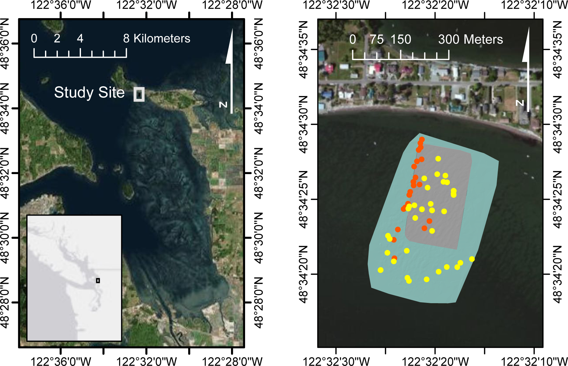
We conducted TLS monitoring in Padilla Bay, a large, shallow bay located north of the Puget Sound in Washington (Figure 1). Padilla Bay measures approximately 13 km north to south, and 5 km east to west and experiences a maximum tidal range of approximately 4 m. Before European settlement, Padilla Bay was a part of the Skagit River distributary system, but subsequent diking and draining of agricultural lands on the Skagit delta have severed this intermittent connection [29]. Turbidity is relatively low in Padilla Bay, with seasonal means varying from 1.8 nephelometric turbidity units (NTU) in the spring to 5.5 NTU in the summer [30]. Extensive intertidal flats in the bay are populated with Z. marina and Z. japonica [31], forming the largest seagrass meadow in the greater Puget Sound [32]. Sub-decimeter vertical scale microtopographic relief in the northern portion of the bay retains water during low tides, creating a mosaic of pools and mounds in the intertidal.
Our study site, in this northern portion of the bay, comprised a 1.84 hectare area of predominantly sandy intertidal sediment, situated between 0.78 and 0.22 m above Mean Lower Low water. Mean Lower Low Water (MLLW), is a tidal elevation datum based on a long-term average of the lowest daily tides at a location. During the year’s lowest low tides, the site would be exposed by the tides for as long as three h.
2.3. TLS Deployment
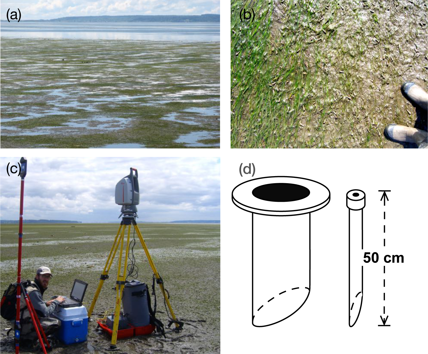
To understand spatial and temporal patterns in intertidal microtopography, we mapped and monitored the study site with a Leica Scanstation II TLS. The Scanstation II is a pulsed laser scanner with a 4 mm laser footprint at 50 m and a nominal range of 300 m at 90% albedo or 134 m at 18% albedo. It can capture up to 50,000 points per second and utilizes a green laser. The scanner is operated through a software interface on a laptop computer, and powered by either alternating or direct current. The TLS incorporates a digital camera that allows coloring the point cloud for visualization purposes, but we found that the image and color quality were inadequate for analysis. We scanned the site during particularly low tides during the spring and summer of 2009, 2010, and 2011, when the tides would uncover the site for 3 h or more.
In order to stabilize the TLS and target poles in the soft, unconsolidated, sediment, we devised inexpensive platforms. Three “tripod anchors” were constructed of 50 cm lengths of 4-inch nominal diameter (10.2 cm) Acrylonitrile Butadiene Styrene (ABS) plumbing pipe and closet flanges (Figure 2). These anchors were driven into the sediment in a configuration that provided three firm resting points for the TLS tripod feet. Target poles were similarly stabilized with anchors created from 50 cm lengths of 2.5 cm diameter Poly Vinyl Chloride (PVC) pipe, fitted with an end cap on one side (Figure 2). A 3 mm hole drilled in the end cap held the spike of the target pole when these anchors were driven into the sediment. Tripod and target anchors could not be left in place between surveys due to hydrodynamic energy at the site.
To minimize disturbance to the soft sediments that we mapped, we attempted to approach the survey location along the same path. Although we undoubtedly had localized impacts on the terrain they were generally small in scope and not visibly persistent between site visits.
The scanner was leveled with a survey tribrach atop a standard survey tripod placed on our tripod anchors. The scanner and laptop computer were powered by a portable gasoline generator or batteries. We utilized the scanner’s dual-axis compensator to ensure that point clouds remained leveled. We acquired four or more scans at each site visit, and combined these by referencing three reflective registration targets (Leica Geosystems HDS twin target poles) common to all acquired scans. Twin target poles were leveled atop the aforementioned target pole anchors, which allowed us to rotate the target poles without altering the location of the reflective target. In 2011, we scanned a larger area (Figure 1), by incorporating additional scans at this adjacent tideflat.
Global Positioning System (GPS) receivers mounted on the target poles allowed for georeferencing of the point clouds. All scans were georeferenced using a survey-grade Global Positioning System (Javad Maxor GGD-T) to facilitate the comparison of topography mapped on different dates. In 2009, we used static GPS observations with carrier-phase differential processing. With this technique, the GPS can provide sub-centimeter nominal accuracy in horizontal and vertical dimensions [33]. In 2010 and 2011, we operated a GPS base station on an adjacent upland location, less than 1 km from the study site, and acquired kinematic GPS locations with GPS rovers. With this technique, the GPS has a nominal accuracy of 11 mm in the horizontal plane and 16 mm vertically [33]. In our usage, the kinematic GPS collection performed better than static GPS, but did not achieve the optimal accuracy suggested by the manufacturer.
Raw TLS point clouds were preprocessed by and georeferenced using Cyclone software (version 7.3, Leica Geosystems, Aarau, Switzerland), and exported to ArcGIS (version 10.0, ESRI, Redlands, CA, USA) for further analysis. Preprocessing consisted of visual identification and removal of erroneous returns, as well as cropping point clouds to exclude points outside of the study area. Because seagrasses lay flat on the sediment when the tide is out, we did not need to filter out erect vegetation from point clouds in order to create a bare-earth model. Next, scans from different viewpoints were registered, and the registered point cloud georeferenced using GPS coordinates from the TLS registration targets. Finally these registered point clouds were exported as text files to be analyzed in ArcGIS. Point clouds were used to create terrain feature classes in ArcGIS, which were subsequently gridded to raster DEMs with a horizontal grain of 10 cm using natural neighbor interpolation. We chose the 10 cm grid resolution as a compromise between detail and file size.
2.4. TLS Validation
In order to validate the ability of TLS to map intertidal microtopographic relief, we compared elevations from georeferenced TLS scans to elevations measured with kinematic GPS receivers. We conducted a GPS survey on 27 July 2011, collecting coordinates at 58 locations in our study site to compare with TLS scans obtained on 19 and 20 April 2011. TLS scans from other years were not explicitly validated in this manner. To prevent the GPS monopod from sinking into the sandy sediments while collecting data, it was placed on thin plastic picnic plate at each survey location. We imported GPS coordinates into our GIS, and extracted elevation values from TLS-derived DEMs in order to compare TLS and GPS derived elevation estimates.
GPS elevations from the 2011 validation survey averaged 2.7 cm (±2.8) cm SD, n = 58) lower than TLS surveys that season, regardless of whether validation points were on pools or mounds (Welch 2 sample t-test, df = 44, p = 0.38). TLS point clouds provided usable terrain data to a range of approximately 50 m from the scanner. At ranges fewer than 10 m from scanner locations, detailed point clouds could easily resolve foot prints and our vegetation sampling quadrats constructed of 2.5 cm diameter PVC tubing.
Using the standard deviation of the error from the validation survey following Brasington et al. [34], Lane et al. [35] and Milan et al. [19], we estimated the Limit of Detection (LoD) for vertical change between our TLS scans. We assumed similar error among our scans, and so estimated a combined uncertainty for a two-scan comparison following [19] by:
2.5. Terrain Analysis
We characterized topographic patterns at the site through semivariogram analysis, Bathymetric Position Index (BPI) mapping, and comparison of DEMs among years. We limited these analyses to the area that was scanned in all three years (Figure 1) We visually examined empirical semivariograms of TLS-derived DEMs to assess the scale of topographic patterns at the site. We first detrended DEM data to account for the overall slope at the site, and then calculated anisotropic empirical semivariograms with a 1 m lag size using the Geostatistical Wizard in ArcGIS 10.1 [37]. We then calculated the slope and the BPI across the site. BPI is the difference of the elevation at a focal point and the mean elevation in a user-specified surrounding neighborhood [38]. Positive values of BPI, thus indicate high points or ridges, negative values depressions, and very small values either flat or uniformly sloping surfaces. By varying the size of the neighborhood, a researcher may inspect the influence of topographic position at multiple scales. Based on our semivariogram inspection (Figure 3), we calculated BPI with 5 and 10 m neighborhood radii.
2.6. Vegetation Distribution
In July 2011, we surveyed vegetation at the study site. Random survey locations were generated in a ArcGIS 10.0, and located in the field to the nearest 5 cm with kinematic GPS. At each survey site we counted all shoots of Z. marina and Z. japonica in a 0.25 m × 0.25 m quadrat and noted the presence of standing water.
These data were combined with TLS generated DEMs and BPI maps to assess the influence of microtopographic context on the presence and density of Z. marina and Z. japonica. We extracted elevations and BPI values at each vegetation sampling location to use as independent variables in our models. The count data were zero-inflated, so we modeled the number of vegetative and generative shoots using a non-parametric, distance based linear modeling technique, DistLM [39,40]. Because we used only a single response variable, and Euclidean distance measurement, the modeling and statistical test is equivalent to a linear model, but p-values are determined via permutations. When multiple predictors were tested, we present r2 values and F-tests for each predictor with all other terms (not including interactions) in the model. For each species we tested the predictive value of the shoot density of the other species, elevation, change in elevation between 2010 and 2011, and BPI from 2009 and 2011.
3. Results
3.1. Terrain Analysis
The monitoring site elevations ranged from 0.22 to 0.78 m above MLLW (Figure 4). The overall slope of the site varied from 0.30% to 0.28% during the course of the study and the overall aspect of the site was southwest, at 210 degrees. Semivariograms revealed directionality of topographic patterns at the site. Perpendicular to the overall slope, semivariance indicates strong spatial patterns at a scale of 6–10 m (Figure 3), but parallel to the slope, patterns were less apparent. Mounds and depressions were generally elongate with their major axis oriented down the slope.
At the site scale, elevation changes between 2009 and 2010 were minimal (Figure 4). The mean difference between 2009 and 2010 DEMs was a loss of just over 2 mm of elevation, this value is more than an order of magnitude smaller than our estimated LoD (8 cm), so we were unable to detect a change at this scale. At the scale of meters, however, elevation changes appeared to be related to microtopographic setting. Elevation change between 2009 and 2010 was inversely correlated with BPI (Pearson’s r =− 0.52), such that mounds were more likely to decrease in elevation and pools more likely to increase in elevation, leading to a less topographically variable site.
These changes were apparent when examining BPI in 2009 and 2010 (Figure 5). The topographic features were less distinct in 2010, although their shape and placement was very similar. BPI in 2010 was positively correlated with BPI in 2009 (Pearson’s r = 0.66), but the slope of the best fit line of 2010 BPI as a function of 2009 BPI was 0.48 ± 0.02, corroborating the decrease the magnitude of topographic relief between 2009 and 2010.
Elevation changes between 2010 and 2011 were again less than our LoD. Localized patterns in elevation change were far less apparent than during the 2009–2010 interval. Elevation change was again negatively correlated with BPI, but less so (Pearson’s r = −0.26). BPI was more correlated between 2010 and 2011 (Pearson’s r = 0.76) than between 2009 and 2010, and the slope of the best-fit line for 2011 BPI as a function of 2010 BPI was closer to one (0.76 ± 0.02).
3.2. Vegetation
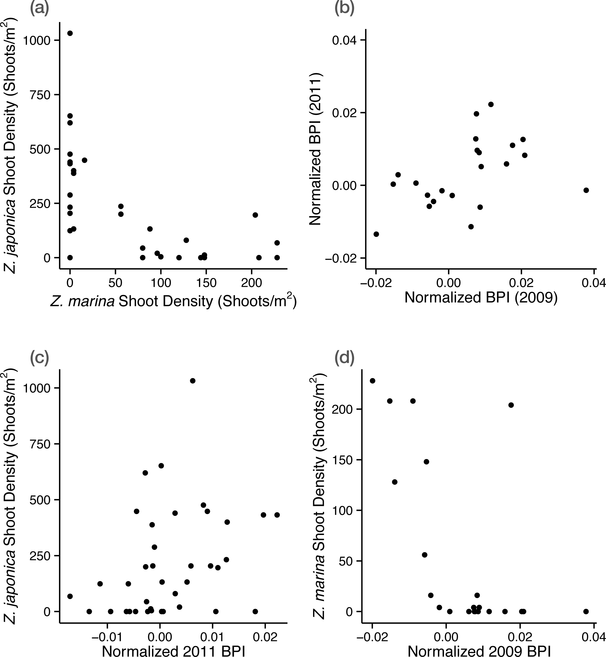
Z. marina and Z. japonica were strongly segregated at the study site, with the highest shoot densities of each species occuring where the other species was sparse or absent (Figure 6). Z. marina tended to be more abundant in locations with negative BPI, and Z. japonica more abundant in locations with positive BPI (Figure 6).
A model with only 2009 BPI explained 35% of the variation in Z. marina shoot density. Z. marina was less dense in areas with higher BPI in 2009 (DistLM, n = 22, 9999 permutations, p = 0.003, r2 = 0.35) and 2011 (DistLM, 9999 permutations, n = 39, p = 0.01, r2 = 0.11). A model with elevation, Z. japonica shoot density, and 2009 BPI explained 59% of the variation in Z. marina shoot density (DistLM, n = 22, 9999 permutations, r2 = 0.59), predicting increased shoot density with lower BPI (r2 = 0.13, p = 0.03) and lower Z. japonica shoot density (r2 = 0.20, p = 0.006).
A model with only BPI explained only 11% of the variation in Z. japonica shoot densities, predicting lower densities where BPI was lower in 2011 (DistLM, 9999 permutations, n = 39, p = 0.04, r2 = 0.11). A model with elevation, 2011 BPI, and Z. marina shoot density explained 50% of the variation in Z. japonica shoot density (DistLM, 9999 permutations, n = 39, r2 = 0.50). Z. japonica grew more densely where Z. marina was less abundant (p = 0.004, r2 = 0.29), and where BPI was greater (p = 0.15, r2 = 0.03).
4. Discussion
4.1. Effectiveness of TLS
We report one of the first uses of TLS on tideflats, and to our knowledge, the first use of TLS to map habitat in this environment. Despite the logistical challenges of deploying TLS equipment in soft sediment intertidal environments, we believe that TLS data are well-suited to the study of patterns and processes in tideflat environments. Topography in these environments is subtle, but due to the influence of tidal inundation, even subtle topography can have profound impacts on resident organisms. Few technologies can successfully capture subtle tideflat topography, with either the resolution or extent of TLS. We succeeded in mapping terrain with sub-decimeter precision and related species cover to centimeter-scale topographic relief at the site, but quantification of temporal change in microtopography proved more difficult.
To maximize the potential of TLS in tideflat studies, it can be integrated with other data collection techniques. Collecting TLS data at the sites of existing topographic monitoring installations, such as SETs, could provide rich spatial context to these fine-scale monitoring techniques. In our application, TLS data could be leveraged by using it to calibrate lower resolution, higher extent data. Based on our semivariogram analysis, imagery with 1–2 m resolution could capture the dominant microtopographic patterns of our study. As such, there is potential to use TLS surveys to calibrate aerial photography or satellite imagery, such as Worldview-3 to expand the extent of mapped habitat. Mobile TLS platforms, operated either from a boat or an unmanned aerial vehicle, could extend the spatial extent of mapping while maintaining high data density.
Our TLS deployment techniques generally performed well at our study site. We saw no evidence of TLS instability affecting our results. Because the TLS operates on a rotating head, if the scanner sunk or shifted during data collection, we would anticipate misalignment artifacts where the start-point and end-point of a scan met. No such artifacts were observed. The Scanstation II incorporates a dual-axis compensator, which was enabled during scanning. This compensates for small deviations from level, and suspends scanning if the scanner shifts far enough that the compensator cannot adjust. For sites with muddier sediment, larger anchors or different stabilizing techniques may be required.
TLS data acquisition may be limited by characteristics of the landscape, and by characteristics of the instrument. Intertidal mudflats are characteristically wet, and periodically submerged. Although saturated sediments did not inhibit data acquisition in this study, standing water did. Pools of standing water greatly reduced TLS return density, and introduced occasional reflection artifacts. This phenomenon has been described in TLS studies of river beds [41], and even capitalized upon to map the water surface in such studies [42]. Point return density may be useful in classifying the TLS image into pools and mounds, particularly by using object-based image analysis to delineate distinct contiguous regions of low point density. TLS has successfully mapped stream bottoms through as much as 20 cm of water [41], but these studies have been limited to small extents within a few meters of the scanner.
One characteristic of our study site, standing water in pools, likely influenced the measured elevations and calculated Bathymetric Position Index. Refraction at the water surface could reduce the accuracy of measured pool bottom elevations. Refraction effects can be corrected [41], but in this study site standing water would first have to be delineated. Pool elevations may have been overestimated by 2–5 cm if TLS returns did not penetrate the water surface due high density of seagrass leaves floating at the pool surface occluding pool bottoms. This would lead to a positive bias in BPI in pools, and a negative bias in BPI on mounds at neighborhood scales large enough to incorporate both water surface and exposed sediment. Although pools at the study site retained water throughout the course of a low tide, we observed that the water level decreased in most pools during low tide exposures. This phenomenon would induce measurement inconsistencies between scans obtained after different durations of low-tide exposure. Such inconsistencies were unlikely to have major impacts on inferences about the influence of microtopographic patterns vegetation distribution, but they add to the challenges of detecting temporal changes in microtopographic relief.
Because of the challenges posed by standing water, our approach to TLS would not be advisable for studying subtidal seagrasses. Bathymetric ALS and acoustic approaches are more promising. While neither are likely to offer the level of detail provided by TLS, subtle microtopography is likely to be less influential in subtidal environments, because ecological importance of tidepools is irrelevant in a continually submerged environment.
A common instrument-specific limitation of TLS is its stationary tripod mount. Due to the fixed vantage point, scanner height limits data acquisition. Because the vertical and horizontal angle between successive scan lines is fixed within a scan, data-point spacing increases as target range increases. This limited our useful scan radius to approximately 50 m. Our implementation of TLS afforded sufficient mapping extent to address the questions of our study, but would not be suitable for larger mapping projects. Some researchers have extended the useful range of scans by elevating the scanner to considerable heights above the sediment surface, e.g., [24], and recently, by developing mobile TLS platforms, e.g., [43].
Another challenge presented by the TLS vantage point is shadowing created by topography or erect vegetation. To overcome this challenge, the researcher may increase the point density of scans in order to penetrate more vegetation gaps, and scan from multiple vantage points. Seagrasses at our study site lie flat on the sediment when the tide is out, and so do not raise more that 2 cm above the sediment surface. Although shadowing was nonexistent in our application due to the gentle nature of site topography and the lack of erect vegetation, it could pose a serious challenge in densely vegetated sites [24].
Quantification of temporal change requires the spatial alignment of scans from different dates. This may be done by scanning persistent, stable landmarks in the study area that can be referenced at different survey dates, or by georeferencing scans from different dates with GPS, as we did. Others have performed TLS surveys of tideflats from adjacent stable, upland areas, e.g., [28]. This approach facilitates the referencing of scans to landmarks, but limits data collection to areas adjacent to stable uplands. GPS allowed us to operate the scanner further from shore, but limited the positioning accuracy that we could achieve.
GPS was the greatest source of positional error in our workflow. Between the first and second year of TLS surveying, we were able to partially mitigate the GPS error with several changes to GPS data collection. In the first year of TLS surveys, a single GPS receiver was available, so scan target locations were obtained by static observations corrected by carrier-phase differential processing. In subsequent years the availability of a second receiver allowed the installation of a base station at the study site during surveys. Scan target locations were obtained by kinematic observations referenced to the nearby base station. Despite the considerable improvement in GPS error afforded by kinematic observations, vertical RMS error of GPS locations was still on the order of centimeters. This level of precision was of a similar scale as observed changes in elevations from year to year, hindering most interpretation of the temporal dynamics of site microtopography and their influence on vegetation. Installation of multiple stable, permanent monuments at the study site would improve precision in future studies. The dynamic nature of an intertidal environment makes this challenging, although approaches developed for SETs [10] could be adapted for this purpose.
4.2. Does Microtopography Predict Seagrass Distribution Patterns?
Microtopographic context was an important predictor of both Z. marina and Z. japonica shoot densities, and shoot densities of each species were inversely correlated. As such, congener shoot density and microtopographic context explained much of the same variance in the models. BPI measurements from 2009 had greater explanatory power than 2011 BPI measurements for both species, but only 2011 measurements were significant for Z. japonica, likely a result of the smaller sample size in 2009 models. This was due to lower TLS return density in 2009, resulting in some ’no data’ cells in BPI maps for that year. The greater explanatory power from the earlier year could be indicative of temporal carry-over effects, but may be due to the greater topographic amplitude in 2009.
Some of the uncertainty in model estimates can be attributed to BPI’s performance as a predictor of mound and pool habitat. BPI is a useful but imperfect predictor of where water will be retained in an intertidal mosaic. A more mechanistic model of water flow off of the tideflat would likely offer better prediction of water retaining sites. Modeling techniques for very low gradient, low relief landscapes such as the study site are less well developed than for higher gradient terrestrial watersheds [44], and would likely require an understanding of subsurface water movement.
Z. marina’s exclusion from sites with high BPI is congruent with observations by Shafer [6], that Z. marina occupies depressions that retain water, and Z. japonica occupies mounds that drain during a low tide. The uncertainty in 2011 BPI coefficient estimates for Z. japonica density may be indicative of a broader microhabitat tolerance at these intertidal elevations. Furthermore, the best predictor of Z. japonica presence, was low shoot densities of Z. marina. Both patterns could result from topographically mediated competitive limitation of Z. japonica to mounds by Z. marina documented by [8].
5. Conclusion
We have demonstrated the potential for Terrestrial Laser Scanner (TLS) mapping of habitat-relevant microtopography in a soft sediment intertidal environment. Furthermore, we have shown the direct relevance of our results for two species of management concern: an invasive seagrass and its native competitor.
Our TLS deployment techniques permitted the mapping of cm-scale topographic relief in an intertidal setting. Despite positioning uncertainty resulting from GPS georeferencing of TLS data we achieved sub-decimeter vertical accuracies. Applying a simple topographic index to TLS-derived digital elevation models revealed that microtopographic patterns at our study site were relatively stable during the three years of study. Installation of stable monuments for georeferencing should yield a far more sensitive change-detection approach.
TLS-derived topographic metrics explained 35% of the variation in shoot density of a native seagrass in an intertidal mixed-species mosaic. Combining TLS-derived elevation, topographic metrics, and shoot densities of the competing species, we could model 59% of the variation in the native seagrass shoot density and 50% of the variation in the invasive seagrass shoot density. With improved change detection ability, TLS could yield insights into the responses of each species to sediment disturbances.
Acknowledgments
Joseph Bracken, Alexandra Kazakova, Justin Kirsch, Jeffery Richardson, Kara Kuhlman, and Suzanne Schull provided assistance in the field. This manuscript benefitted from helpful reviews by Aaron Johnston, Jeffery Richardson, Meghan Halabisky, Peter Dowty, and three anonymous reviewers. This research was conducted in the National Estuarine Research Reserve System under an award from the Estuarine Reserves Division, Office of Ocean and Coastal Resource Management, National Ocean Service, National Oceanic and Atmospheric Administration. The TLS was purchased through a Student Technology Fee Grant from the University of Washington.
Author Contributions
MH conceived of the study with advice from LMM. MH and LMM carried out data collection. LMM provided equipment and analysis tools. MH wrote manuscript with review and input from LMM.
Conflicts of Interest
The authors declare no conflict of interest.
References
- Horn, H.S.; Arthur, R.H.M. Competition among fugitive species in a harlequin environment. Ecology 1972, 53, 749–752. [Google Scholar]
- Tamme, R.; Hiiesalu, I.; Laanisto, L.; Szava-Kovats, R.; Pärtel, M. Environmental heterogeneity, species diversity and co-existence at different spatial scales. J. Veg. Sci. 2010, 21, 796–801. [Google Scholar]
- Garrity, S.D. Some adaptations of gastropods to physical stress on a tropical rocky shore. Ecology 1984, 65, 559–574. [Google Scholar]
- Wyer, D.W.; Boorman, L.A.; Waters, R. Studies on the distribution of Zostera in the outer Thames Estuary. Aquaculture 1977, 12, 215–227. [Google Scholar]
- Harrison, P.G. Spatial and temporal patterns in abundance of two intertidal seagrasses, Zostera americana Den Hartog and Zostera marina L. Aquat. Bot. 1982, 12, 305–320. [Google Scholar]
- Shafer, D.J.; Physiological, Factors. Affecting the Distribution of the Nonindigenous Seagrass Zostera Japonica along the Pacific Coast of North America. Ph.D. Thesis, University of South Alabama, Mobile, AL, USA, 2007. [Google Scholar]
- Van der Heide, T.; Eklöf, J.S.; van Nes, E.H.; van der Zee, E.M.; Donadi, S.; Weerman, E.J.; Olff, H.; Eriksson, B.K. Ecosystem engineering by seagrasses interacts with grazing to shape an intertidal Landscape. PLoS One 2012, 7, e42060. [Google Scholar]
- Hannam, M.; Wyllie-Echeverria, S. Microtopography promotes coexistence of an invasive seagrass and its native congener. Biol. Invasions. 2015, 17, 381–395. [Google Scholar]
- Shafer, D.J.; Sherman, T.D.; Wyllie-Echeverria, S. Do desiccation tolerances control the vertical distribution of intertidal seagrasses? Aquat. Bot. 2007, 87, 161–166. [Google Scholar]
- Boumans, R.; Day, J. High precision measurements of sediment elevation in shallow coastal areas using a sedimentation-erosion table. Estuaries Coasts. 1993, 16, 375–380. [Google Scholar]
- Bos, A.R.; Bouma, T.J.; de Kort, G.; van Katwijk, M.M. Ecosystem engineering by annual intertidal seagrass beds: Sediment accretion and modification. Estuar. Coast. Shelf Sci. 2007, 74, 344–348. [Google Scholar]
- Chust, G.; Galparsoro, I.; Borja, Á.; Franco, J.; Uriarte, A. Coastal and estuarine habitat mapping, using LIDAR height and intensity and multi-spectral imagery. Estuar. Coast. Shelf Sci. 2008, 78, 633–643. [Google Scholar]
- Milan, D.J.; Heritage, G.L. LiDAR and ADCP use in gravel-bed rivers: Advances since GBR6. In Gravel-Bed Rivers: Processes, Tools, Environments; Church, M., Biron, P.M., Roy, A.G., Eds.; John Wiley & Sons: Chichester, UK, 2012; pp. 1–29. [Google Scholar]
- Brock, J.C.; Clayton, T.D.; Nayegandhi, A.; Wright, C.W. LIDAR optical rugosity of coral reefs in Biscayne National Park, Florida. Coral Reefs. 2004, 23, 48–59. [Google Scholar]
- Valle, M.; Borja, Á.; Chust, G.; Galparsoro, I.; Garmendia, J.M. Modelling suitable estuarine habitats for Zostera noltii, using ecological niche factor analysis and bathymetric LiDAR. Estuar. Coast. Shelf Sci. 2011, 94, 144–154. [Google Scholar]
- Collin, A.; Long, B.; Archambault, P. Salt-marsh characterization, zonation assessment and mapping through a dual-wavelength LiDAR. Remote Sens. Environ. 2010, 114, 520–530. [Google Scholar]
- Irish, J.L.; Lillycrop, W.J. Scanning laser mapping of the coastal zone: The SHOALS system. ISPRS J. Photogramm. Remote Sens. 1999, 54, 123–129. [Google Scholar]
- Quadros, N.D.; Collier, P.A.; Fraser, C.S. Integration of bathymetric and topographic LiDAR: a preliminary investigation. Remote Sens. Spat. Inf. Sci. 2008, 37, 1299–1304. [Google Scholar]
- Milan, D.J.; Heritage, G.L.; Hetherington, D. Application of a 3D laser scanner in the assessment of erosion and deposition volumes and channel change in a proglacial river. Earth Surf. Process. Landf. 2007, 32, 1657–1674. [Google Scholar]
- Vierling, K.T.; Vierling, L.A.; Gould, W.A.; Martinuzzi, S.; Clawges, R.M. Lidar: Shedding new light on habitat characterization and modeling. Front. Ecol. Environ. 2008, 6, 90–98. [Google Scholar]
- Fröhlich, C.; Mettenleiter, M. Terrestrial laser scanning–New perspectives in 3D surveying. Int. Arch. Photogramm. Remote Sens. Spat. Inf. Sci. 2004, 36, 7–18. [Google Scholar]
- Clawges, R.M.; Vierling, L.; Calhoon, M.; Toomey, M. Use of a ground-based scanning Lidar for estimation of biophysical properties of western Larch (Larix Occidentalis). Int. J. Remote Sens. 2007, 28, 4331–4344. [Google Scholar]
- Zheng, G.; Moskal, L.M.; Kim, S.H. Retrieval of effective leaf area index in heterogeneous forests with Terrestrial Laser Scanning. IEEE Trans. Geosci. Remote Sens. 2013, 51, 777–786. [Google Scholar]
- Anderson, K.; Bennie, J.; Wetherelt, A. Laser scanning of fine scale pattern along a hydrological gradient in a peatland ecosystem. Landsc. Ecol. 2010, 25, 477–492. [Google Scholar]
- Bennie, J.; Anderson, K.; Wetherelt, A. Measuring biodiversity across spatial scales in a raised bog using a novel paired-sample diversity index. J. Ecol. 2011, 99, 482–490. [Google Scholar]
- Guarnieri, A.; Vettore, A.; Pirotti, F.; Menenti, M.; Marani, M. Retrieval of small-relief marsh morphology from Terrestrial Laser Scanner, optimal spatial filtering, and laser return intensity. Geomorphology 2009, 113, 12–20. [Google Scholar]
- Hetherington, D.; German, S.; Utteridge, M.; Cannon, D.; Chisholm, N.; Tegzes, T. Accurately representing a complex estuarine environment using Terrestrial Lidar, Proceedings of the RSPSoc Conference, Newcastle Upon Tyne, UK, 11–14 September 2007.
- Thiebes, B.; Wang, J.; Bai, S.; Li, J. Terrestrial laserscanning of tidal flats—A case study in Jiangsu Province, China. J. Coast. Conserv. 2013, 17, 813–823. [Google Scholar]
- National Ocean Survey (NOS)Washington State Department of Ecology (WSDE)Draft Environmental Impact Statement, Padilla Bay Estuarine Sanctuary; Technical Report; NOS: Washington, DC, USA; WSDE: Olympia, WA, USA, 1980.
- Bulthuis, D. Review of Water Quality Data in the Padilla Bay/Bayview Watershed; Technical Report 10; Washington: Dept. Ecology, Padilla Bay NERR: Mount Vernon, WA, USA, 1993. [Google Scholar]
- Bulthuis, D. Coastal Habitats in Padilla Bay, Washington A Review; Technical Report; Washington Dept. Ecology, Padilla Bay NERR: Mount Vernon, WA, USA, 1996. [Google Scholar]
- Berry, H.; Sewell, A.T.; Wyllie-Echeverria, S.; Reeves, B.; Mumford, T.; Skalski, J.R.; Zimmerman, R.; Archer, J. Puget Sound Submerged Vegetation Monitoring Project: 2000–2002 Monitoring Report; Technical Report; Nearshore Habitat Program, Washington DNR: Olympia, WA, USA, 2003. [Google Scholar]
- JNS Support Team. Maxor-GGDT Operators Manual; JNS Support Team: San Jose, CA, USA, 2006. Available online: http://www.javad.com/downloads/jns/manuals/hardware/Maxor-GGDT%20Operators%20Manual.pdf accessed on 15 February 2015.
- Brasington, J.; Rumsby, B.T.; McVey, R.A. Monitoring and modelling morphological change in a braided gravel-bed river using high resolution GPS-based survey. Earth Surf. Process. Landf. 2000, 25, 973–990. [Google Scholar]
- Lane, S.N.; Westaway, R.M.; Murray Hicks, D. Estimation of erosion and deposition volumes in a large, gravel-bed, braided river using synoptic remote sensing. Earth Surf. Process. Landf. 2003, 28, 249–271. [Google Scholar]
- Milan, D.J.; Heritage, G.L.; Large, A.R.G.; Fuller, I.C. Filtering spatial error from DEMs: Implications for morphological change estimation. Geomorphology 2011, 125, 160–171. [Google Scholar]
- ESRI, ArcGIS 9.2; ESRI: Redlands, CA, USA, 2006.
- Lunblad, E.R. The Development and Application of Benthic Classifications for Coral Reef Ecosystems Below 30 m Depth using Multibeam Bathymetry: Tutuila, American Samoa. Ph.D. Thesis, Oregon State University, Corvallis, OR, USA, 2004. [Google Scholar]
- Anderson, M.J.; Robinson, J. Permutation tests for linear models. Aust. N. Z. J. Stat. 2001, 43, 75–88. [Google Scholar]
- Anderson, M.J. Permutation tests for univariate or multivariate analysis of variance and regression. Can. J. Fish. Aquat. Sci. 2001, 58, 626–639. [Google Scholar]
- Smith, M.; Vericat, D.; Gibbins, C. Through-water Terrestrial Laser Scanning of gravel beds at the patch scale. Earth Surf. Process. Landf. 2012, 37, 411–421. [Google Scholar]
- Milan, D.J.; Heritage, G.L.; Large, A.R.G.; Entwistle, N.S. Mapping hydraulic biotopes using Terrestrial Laser Scan data of water surface properties. Earth Surf. Process. Landf. 2010, 35, 918–931. [Google Scholar]
- Alho, P.; Kukko, A.; Hyyppä, H.; Kaartinen, H.; Hyyppä, J.; Jaakkola, A. Application of boat-based laser scanning for river survey. Earth Surf. Process. Landf. 2009, 34, 1831–1838. [Google Scholar]
- Jones, K.L.; Poole, G.C.; O’Daniel, S.J.; Mertes, L.A.K.; Stanford, J.A. Surface hydrology of low-relief Landscapes: Assessing surface water flow impedance using LIDAR-derived digital elevation models. Remote Sens. Environ. 2008, 112, 4148–4158. [Google Scholar]


| Source | Magnitude, Direction | Possible Mitigation Strategies |
|---|---|---|
| Pool surface, leaf reflection | up to +5 cm | Scan in winter, increase incidence angle |
| GPS georeferencing | ±3 cm SD | Install stable monuments |
| Vegetation on mounds | up to +5 cm | Scan in winter |
| Tidepool drainage | up to 5 cm | Measure tidepool water depth |
© 2015 by the authors; licensee MDPI, Basel, Switzerland This article is an open access article distributed under the terms and conditions of the Creative Commons Attribution license (http://creativecommons.org/licenses/by/4.0/).
Share and Cite
Hannam, M.; Moskal, L.M. Terrestrial Laser Scanning Reveals Seagrass Microhabitat Structure on a Tideflat. Remote Sens. 2015, 7, 3037-3055. https://doi.org/10.3390/rs70303037
Hannam M, Moskal LM. Terrestrial Laser Scanning Reveals Seagrass Microhabitat Structure on a Tideflat. Remote Sensing. 2015; 7(3):3037-3055. https://doi.org/10.3390/rs70303037
Chicago/Turabian StyleHannam, Michael, and L. Monika Moskal. 2015. "Terrestrial Laser Scanning Reveals Seagrass Microhabitat Structure on a Tideflat" Remote Sensing 7, no. 3: 3037-3055. https://doi.org/10.3390/rs70303037